Extra-galactic background light measurements from the far-UV to the far-IR from deep ground and space-based galaxy counts

Abstract

We combine wide and deep galaxy number-count data from GAMA, COSMOS/G10, HST ERS, HST UVUDF and various near-, mid- and far- IR datasets from ESO, Spitzer and Herschel. The combined data range from the far-UV (0.15$\mu$m) to far-IR ($500\mu$m), and in all cases the contribution to the integrated galaxy light (IGL) of successively fainter galaxies converges. Using a simple spline fit, we derive the IGL and the extrapolated-IGL in all bands. We argue undetected low surface brightness galaxies and intra-cluster/group light is modest, and that our extrapolated-IGL measurements are an accurate representation of the extra-galactic background light. Our data agree with most earlier IGL estimates and with direct measurements in the far-IR, but disagree strongly with direct estimates in the optical. Close agreement between our results and recent very high-energy experiments (H.E.S.S. and MAGIC), suggest that there may be an additional foreground affecting the direct estimates. The most likely culprit could be the adopted Zodiacal light model. Finally we use a modified version of the two-component model to integrate the EBL and obtain measurements of the Cosmic Optical Background (COB) and Cosmic Infrared Background (CIB) of: $24^{+4}_{-4}$ nW m^-2 sr^-1 and $26^{+5}_{-5}$ nW m^-2 sr^-1 respectively (48:52%). Over the next decade, upcoming space missions such as Euclid and WFIRST, have the capacity to reduce the COB error to $<1\%$, at which point comparisons to the very high energy data could have the potential to provide a direct detection and measurement of the reionisation field.

1. Introduction

The extra-galactic background light, or EBL (McVittie & Wyatt, 1959; Partridge & Peebles, 1967a; Partridge & Peebles, 1967b; Hauser & Dwek, 2001; Lagache et al., 2005; Kashlinsky, 2006; and Dwek & Krennrich, 2013), represents the flux received today from a steradian of extragalactic sky. It includes all far-UV to far-IR sources of photon production since the era of recombination, and thereby encodes a record of the entire energy production history of the Universe from $\sim$380,000yrs after the Big Bang to the present day — see Wesson et al. (1987) and Wesson (1991) for an interesting digression regarding the EBL’s relation to Olber’s Paradox. By convention, the EBL is defined as the radiation received between 0.1$\mu$m to 1000$\mu$m (e.g., Finke et al., 2010, Domínguez et al., 2011; Dwek & Krennrich, 2013; Khaire & Srianand, 2015). This arises predominantly from star-light, AGN-light, and dust reprocessed light — with some minimal ($<15\%$) contribution from direct dust heating due to accretion (Alexander et al., 2005; Jauzac et al., 2011). Photon production occurs not only at far-UV to far-IR wavelengths, but across the entire electro-magnetic spectrum (e.g., the cosmic x-ray background, see Shanks et al., 1991; and the cosmic radio background, see de Oliveira-Costa et al., 2008). However, based on integrated energy considerations (i.e., $\int_{z=0}^{z=1050}\int^{\nu_{2}}_{\nu_{1}}\nu f_{\nu}\ \delta\nu\ \delta z$), the cosmic emission is dominated, in terms of newly minted photons, by the far-UV to far-IR range. Compared to the Cosmic Microwave Background (CMB) the integrated-EBL is smaller by a factor of $\sim 20$, despite the $(1+z)^{4}$ diminution of the CMB photon energies, but more than a factor of $\times 100$ brighter than the other backgrounds. Putting aside the CMB and the pre-recombination Universe, the EBL is a product of the dominant astrophysical processes which have taken place over the past 13 billion years, in terms of energy redistribution (baryonic mass $\rightarrow$ photons). In particular, because of the expansion, the precise shape of the spectral energy distribution of the EBL depends on the cosmic star-formation history, AGN activity history, and the evolution of dust properties over cosmic time. It therefore represents rich territory for comparison to galaxy formation and evolution models (e.g., Domínguez et al., 2011; Somerville et al., 2012; Inoue et al., 2013).

The EBL can be broken down into two roughly equal contributions from the UV-optical-near-IR and the mid- to far- IR wavelength ranges: the Cosmic Optical Background (COB; 0.1$\mu$m — 8$\mu$m) and the Cosmic Infrared Background (CIB $8\mu$m — 1000$\mu$m; Dwek et al., 1998). Despite the different wavelength ranges, the COB and CIB ultimately derive from the same origin: star-formation and gravitational accretion onto super-massive black holes. The COB represents the star- and AGN- light which directly escapes the host system, and obsequiously pervades into the inter-galactic medium. The CIB represents that component which is first attenuated by dust near the radiation sources, and subsequently re-radiated in the mid- and far-IR. The near equal balance between the energy of the integrated COB and CIB is very much a testimony to the severe impact of dust attenuating predominantly UV and optical photons, particularly given the very modest amount of baryonic mass in the form of dust ($<1$% relative to stellar mass, see for example Driver et al., 2008; Dunne et al., 2011).

Previous measurements of the EBL have come two flavours: direct measurements (e.g., Puget et al., 1996; Fixsen et al., 1998; Dwek & Arendt, 1998; Hauser et al., 1998; Lagache et al., 1999; Dole et al., 2006; Bernstein et al., 2002; Bernstein, 2007; Cambrésy et al., 2001; Matsumoto et al., 2005; Matsumoto et al., 2011) and integrated galaxy-counts (e.g., Madau & Pozzetti, 2000; Hopwood et al., 2010; Xu et al., 2005; Totani et al., 2001; Dole et al., 2006; Keenan et al., 2010; Berta et al., 2011; Béthermin et al., 2012). These two methods should converge if the EBL is predominantly derived from galaxies (including any AGN component), and if the photometric data used to detect these galaxies are sufficiently deep.

Until fairly recently, insufficient deep data existed to completely resolve the EBL using galaxy number-counts, and direct measurements appeared the more compelling constraint. However, with the advent of space-based facilities (GALEX, HST, Spitzer and Herschel), and large ground-based facilities (VLT, Subaru), deep field data have now been obtained across the entire far-UV to far-IR range. The comparison of the direct estimates and integrated number-counts are proving fertile ground for debate. In the CIB, the direct estimates agree reasonably well with the integrated source counts, which account for over 75% of the directly measured CIB (see Béthermin et al., 2012 and Magnelli et al., 2013). The remaining discrepancy can be readily reconciled from extrapolations of the source counts, plus some additional contribution from lensed systems (Wardlow et al., 2013). In the optical and near-IR the situation is less clear, with many direct estimates being a factor of five or more greater than the integrated galaxy counts (see for example the discussion on the near-IR background excess in Keenan et al., 2010 or Matsumoto et al., 2015), despite the advent of very wide and deep data. Either the integrated source counts are missing a significant quantity of the EBL in a diffuse component, or the direct measures are over-estimated (i.e., the backgrounds are under-estimated).

Recently a third pathway to the EBL has opened up, via the indirect attenuation of TeV photons emanating from Blazars, as observed with Very High Energy (VHE) experiments (e.g., the High Energy Stereoscopic System, H.E.S.S., and the Major Atmospheric Gamma Imaging Cherenkov telescope, MAGIC). Here the TeV flux from a distant Blazar, believed to extrude a well behaved power-law spectrum, interacts with the intervening EBL photon-field. Preferential interactions between TeV and micron photons create electron-positron pairs, thereby removing power from the received TeV spectrum over a characteristic wavelength range. The proof of concept was demonstrated by Aharonian et al. (2006) and comprehensive measurements have recently been made by both the H.E.S.S. Consortium (H.E.S.S. Collaboration et al., 2013) and the MAGIC team (Ahnen et al., 2016). These two independent measurements very much favour the low-EBL values. However, uncertainty remains as to the strength, and hence, impact of the inter-galactic magnetic field, the intrinsic Blazar spectrum shape, and the role of secondary PeV cascades. Moreover, the two VHE studies mentioned above require a pre-defined EBL model, and use the shape of the received TeV signal compared to the assumed intrinsic spectrum, to provide a normalisation point. Hence spectral information is essentially lost. Trickier to determine but more powerful is the potential for the VHE data to constrain both the normalisation and the shape of the EBL spectrum. A first effort was recently made by Biteau & Williams (2015) who again found results consistent with the low-EBL value, but perhaps more crucially provided independent confirmation of the overall shape across the far-UV to far-IR wavelength range. Nevertheless, caveats remain as to the true intrinsic Blazar spectral slope in the TeV range, contaminating cascades from PeV photons, the strength of any intervening magnetic fields, and in some cases the actual redshift of the Blazars studied.

Here we aim to provide the first complete set of integrated-galaxy light measurements based on a combination of panchromatic wide and deep number/source-count data from a variety of surveys which collectively span the entire EBL wavelength range (0.1$\mu$m — 1000$\mu$m). Our approach varies from previous studies, in that we abandon the concept of modeling the data with a galaxy-count (backward propagation) model. Instead, as the number-count data is bounded in all bands — in terms of the contribution to the integrated luminosity density — we elect to fit a simple spline to the luminosity density data.

In Section 2, we present the adopted number-count data, the trimming required before fitting, and estimates of the cosmic (sample) variance associated with each dataset. In Section 3, we describe our fitting process and the associated error analysis. We compare our measurements to previous estimates in Section 4, including direct and VHE constraints, before exploring possible sources of missing light. We finish by using the EBL model of Driver & Andrews (see Driver et al., 2013 and Andrews et al., 2016b) as an appropriate fitting function to derive the total integrated energy of the COB and CIB.

All magnitudes are reported in the AB system, and where relevant we have used a cosmology with $\Omega_{\Lambda}=0.7,\Omega_{\rm Matter}=0.3$, and, $H_{o}=70$km/s/Mpc.

2. Number-count data

This work has been motivated by the recent availability of a number of panchromatic data sets which extend from the far-UV to the far-IR. In particular: Galaxy And Mass Assembly (GAMA) (Driver et al., 2011; Driver et al., 2016a; Liske et al., 2015; Hopkins et al., 2013); COSMOS/G10 (Davies et al., 2015; Andrews et al., 2016a); Hubble Space Telescope Early Release Science (ERS; Windhorst et al., 2011); and the Hubble Space Telescope Ultra-Violet Ultra-Deep Field (UVUDF; Teplitz et al., 2013, Rafelski et al., 2015). For each of these datasets great care has been taken to produce consistent and high quality photometry across a broad wavelength range. We have been responsible for the production of the first three catalogues, with the fourth recently made publicly available. We describe the various datasets in more detail below.

2.1. Galaxy And Mass Assembly (GAMA)

GAMA represents a survey of five sky regions covering 230 $\deg^{2}$ (Driver et al., 2011), with spectroscopic data to $r=19.8$mag obtained from the Anglo-Australian Telescope (Liske et al., 2015). Complementary panchromatic imaging data comes from observations via GALEX (Liske et al., 2015), SDSS (Hill et al., 2011), VISTA (Driver et al., 2016a), WISE (Cluver et al., 2014), and Herschel (Eales et al., 2010, Valiante et al., 2016). The GAMA Panchromatic Data Release imaging (Driver et al., 2016a) was made publicly available in August 2015 (http://gama-psi.icrar.org). The 180 $\deg^{2}$ which makes up the three GAMA equatorial regions (G09, G12 & G15), has since been processed with the custom built panchromatic analysis code lambdar (Wright et al., 2016), to derive matched-aperture and PSF-convolved photometry across all bands. The Wright-catalogue is $r$-band selected using SExtractor (Bertin & Arnouts, 1996). The SExtractor-defined apertures are convolved with the appropriate point-spread function for each facility, and used to derive consistent flux measurements in all other bands. Care is taken to manage overlapping objects and flux share appropriately (see Wright et al., 2016 for full details). As part of the quality control process, all bright and all oversized apertures (for their magnitude), were visually inspected and corrected if necessary. The Wright-catalogue then uses these apertures to provide fluxes in the following bands: FUV/NUV, $ugri$, $ZYJHK$, $IRAC$-$1/2/3/4$, PACS 100/160, SPIRE 250/350/500. Number-counts are generated by binning the data within 0.5mag intervals and scaling for the area covered. Random errors are derived assuming Poisson statistics (i.e., $\sqrt{n}$) with cosmic variance errors included in the analysis as described in Sections 2.5 and 3.3.4. Note that in generating number counts, the $r$-band selection will lead to a gradual flattening of the counts in other bands, particularly those bands furthest in wavelength from $r$, i.e., a colour bias. The very simple strategy we adopt here is to identify the point at which the GAMA Wright-catalogue counts diverge from the deeper datasets and truncate our counts 0.5 mag brightwards of this limit. See Wright et al. (2016) for full details of the GAMA analysis including aperture verification.

2.2. COSMOS/G10

COSMOS/G10 represents a complete reanalysis of the available spectroscopic and imaging data to GAMA standards, in a 1 sq. degree region of the HST COSMOS field (Scoville et al., 2007), dubbed G10 (GAMA $10^{h}$; see Davies et al., 2015, Andrews et al., 2016a for full details). The primary source detection catalogue uses SExtractor applied to deep Subaru $i$-band data, following trial and error optimisation of the SExtractor detection parameters. All anomalous apertures were manually inspected and repaired, as needed. As for GAMA, the lambdar software was used to generate matched aperture photometry from the far-UV to far-IR. The photometry for the COSMOS/G10 region spans 38 wavebands, and combines data from GALEX (Zamojski et al., 2007), CFHT (Capak et al., 2007), Subaru (Taniguchi et al., 2007), VISTA (McCracken et al., 2012), Spitzer (Sanders et al., 2007 and Frayer et al., 2009) and Herschel (Lutz et al., 2011, Oliver et al., 2012, Levenson et al., 2010, Viero et al., 2013, Smith et al., 2012 and Wang et al., 2014). As for GAMA the number-counts are derived in 0.5mag bins yielding counts in: FUV/NUV, u, griz, YJHK, $IRAC1/2/3/4$, MIPS 24/70, PACS 100/160, SPIRE 250/350/500. The COSMOS/G10 catalogue is $i$-band selected, and hence a gradual decline in the number counts will occur in filters other than $i$, as either very red or blue galaxies are preferentially lost. In particular, a cascading flux cut was implemented as the optical priors were advanced into the far-IR to minimise erroneous measurements. As for GAMA we use the departure of the COSMOS/G10 counts from the available deeper data to identify the magnitude limits at which the counts become incomplete. See Andrews et al. (2016a) for full details of the COSMOS/G10 analysis including data access.

2.3. Hubble Space Telescope Early Release Science (HST ERS)

The HST ERS dataset (Windhorst et al., 2011) represents one of the first fields obtained using HST’s WFC3, and built upon earlier optical ACS imaging of the GOODS South field. The analysis details are provided in Windhorst et al (2011), and counts are derived in 11 bands: F225W, F275W, F306W, F435W, F775W, F850LP, F098M, F105W, F125W, F140W, and F160W covering 40-50 arcmin² to AB $26.3$—$27.5$ mag. For the HST ERS, data catalogues were derived independently in each band, hence avoiding any color bias. Spitzer and Herschel data exists for the HST ERS field, but is currently not part of this analysis due to its much coarser beam and the resulting faint-end confusion. In due course, we expect to reprocess the ERS data using lambdar. In addition to the HST ERS field the ASU team have also measured deep counts in various bands in the UDF and XDF fields using an identical process as that described for the HST ERS data, but including a correction for incompleteness by inserting false galaxy images into real data and assessing the fraction recovered as a function of magnitude. See Windhorst et al. (2011) for full details of the HST ERS and deep field analysis.

2.4. Hubble Space Telescope ultra-violet ultra-deep field (HST UVUDF)

The HST UVUDF dataset (Teplitz et al., 2013) represents a major effort to bring together data on the HUDF field spanning a broad wavelength range and consisting of 11 bands from the near-UV to the near-IR (see Rafelski et al., 2015). The UVUDF team also use an aperture matched point-spread function corrected method to derive the photometry. The area of coverage varies from 7.3 to 12.8 arcmin² across the bands. The initial detection image is derived from the combination of 4 optical and 4 near-IR bands (weighted by the inverse variance of each image on a pixel-by-pixel basis). As the near-IR data is variable in depth, this does produce a catalogue with a slightly variable detection wavelength. However, the basic strategy of object detection based on multi-filter stacked data combined with pixel weighting, should mitigate most of the color selection bias in the count data. The Rafelski et al. catalogue is publicly available and counts are derived by binning the data in 0.5mag intervals and scaling for area. The HST UVUDF dataset contains counts in the following bands: F225W, F275W, F336W, F435W, F606W, F775W, F850LP, F105W, F125W, F140W, and F160W. See Rafelski et al. (2015) for full details of the UVUDF data analysis.

2.5. Additional datasets & cosmic variance (CV)

In addition to the four primary catalogues mentioned above, we include a number of band specific surveys to extend the range of our number count analysis into the far-UV, mid-IR and far-IR. These datasets, along with the four primary datasets, are summarised in Table 1. All datasets will be susceptible to cosmic variance particularly at the fainter ends of the HST datasets, where the volumes probed will be very small. For each dataset we therefore derive a cosmic (sample) variance error; listed in Col. 5 of Table 1 using equation 4 from Driver & Robotham (2010). These values are based on the quoted field-of-view, the number of independent fields, and an assumed redshift distribution and the adopted values are also shown in Table. 1. We refer the curious reader to our online calculator: http://cosmocalc.icrar.org (see Survey Design tab).

Table 1A summary of datasets used in this analysis and in particular the cosmic variance errors estimated via Eqn 4 from Driver & Robotham (2010), see also http://cosmocalc.icrar.org for our online calculator.

Filter	Description	$\Omega$	z	CV	Reference
		($\deg^{2}$)	range	(%)
All	GAMA 21 band panchromatic data release	$3\times 60$	0.05—0.30	5%	Wright et al. (2016)
All	COSMOS/G10 38 band panchromatic data release	1	0.2—0.8	11%	Andrews et al. (2016a)
UV-NIR	HST WFC3 Early Release Science (Panchromatic Counts)	0.0125	0.5—2.0	17%	Windhorst et al. (2011)
UV-NIR	HST Ultra-violet through NIR observations of the Hubble UDF	0.0036	0.5—2.0	21%	Rafelski et al. (2015)
FUV	HST ACS Solar Blind Channel observations of HDF-N(GOODS-S), HUDF, GOODS-N	$3\times\sim 0.0015$	0.5—2.0	14%	Voyer et al. (2011)
NUV	STIS observations in the HDF-N, HDF-S, and the HDF-parallel	$3\times\sim 0.00012$	0.5—2.0	21%	Gardner et al. (2000)
$u$	near-UV(360nm) observations in the Q0933+28 field with the Large Binocular Camera	0.4	0.5—2.0	8%	Grazian et al. (2009)
$K$	The Hawk-I UDS and GOODS Survey (HUGS)	0.016, 0.078	0.5—2.0	11%	Fontana et al. (2014)
$IRAC$-$1/2$	S-CANDELS: The Spitzer-Cosmos Assembly Near Infrared Deep Extragalactic Survey: 3.6 and 4.5 $\mu$m Spitzer IRAC	$5\times\sim 0.032$	0.5—2.0	6%	Ashby et al. (2015)
$IRAC$-$4$(8$\mu$m)	Spitzer IRAC Band 4 data of the EGS field	0.38	0.5—2.0	8%	Barmby et al. (2008)
$24\mu$m	Spitzer MIPS 24$\mu$m observations of Marano, CDF-S, EGS, Boötes and ELAIS fields	0.36,0.58,0.41,9.0,0.036	0.5—2.0	3%	Papovich et al. (2004)
$24\mu$m	Spitzer MIPS 24$\mu$m data in FIDEL, COSMOS and SWIRE fields	53.6 (9 fields)	0.5—2.0	2%	Béthermin et al. (2010)
$70/160\mu$m	Spitzer MIPS 70 & 160 $\mu$m data	45.4 (9 fields)	0.5—2.0	2%	Béthermin et al. (2010)
$70\mu$m	Herschel PACS 70 $\mu$m data	42.9 (9 fields)	0.5—2.0	2%	Béthermin et al. (2010)
$100/160\mu$m	Herschel The PACS Evolutionary Probe Survey (100 & 160 $\mu$m data) of the GOODS-S, GOODS-N, Lockman Hole and COSMOS areas	0.083,0.083,0.18,2.04	0.5—2.0	5%	Berta et al. (2011)
$100/160\mu$m	Herschel PACS 100 & 160 $\mu$m data from PEP and GOODS-Herschel campaigns	$2\times\sim 0.052$	0.5—2.0	9%	Magnelli et al. (2013)
$250/350/500\mu$m	Herschel (HerMES) SPIRE 250, 350 & 500 $\mu$m observations in the COSMOS and GOODS-N regions	0.083,2.04	0.5—2.0	5%	Béthermin et al. (2012)
$250/350/500\mu$m	Herschel (H-Atlas) SPIRE 250, 350 & 500 $\mu$m observations in the equatorial GAMA fields	$3\times 54$	0.05—2.0	2%	Valiante et al. (2016)

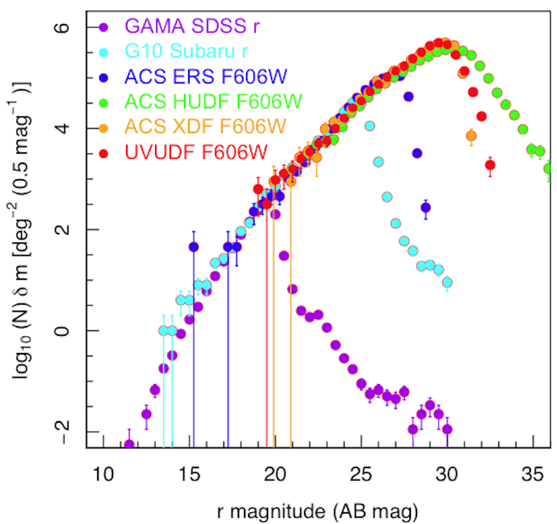
Figure 1.— $r$-band number counts produced by simply combining the catalogues as provided. Each dataset shows a clear down-turn of the number counts at faint magnitudes, which is an artifact of the flux and color limit of that dataset. To correct for this, we truncate each dataset 0.5 mag brightwards of its turn-down point. In some cases we also truncate bright data, when the errorbars become excessive, and would have no impact on our fitting whether included or not.

2.6. Merging datasets

Fig. 1 shows the combined galaxy number counts in the $r$ band from six datasets of varying areas and depths. The figure highlights the distinct limits of each dataset reflected by the abrupt turn-downs. Care must therefore be taken to truncate each dataset at an appropriate magnitude limit. For the GAMA and COSMOS/G10 datasets we identify the turn-down as the point at which the data become inconsistent with the deeper datasets. This is because the colour bias introduces a shallow rather than abrupt turn-down. For all other datasets we identify the point at which the counts at faint magnitudes fall abruptly, and then truncate 0.5 mag brightwards. Truncating in this way results in a fairly seamless distribution (see Fig. 2, top left panel).

Our final number-count distributions, for three arbitrarily selected bands ($r$, $IRAC$-$1$ and SPIRE $250\mu$m), are shown in Fig. 2 (left panels). Following the trimming process, the datasets shown overlap extremely well.

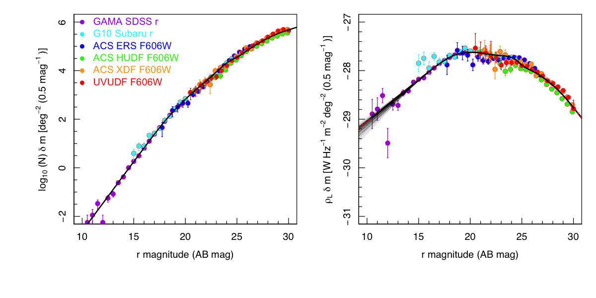
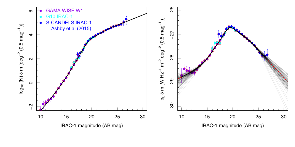
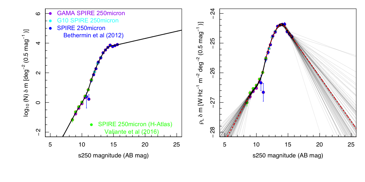
Figure 2.— (left) Galaxy number counts in the specified band, where the black curve depicts the 10-point spline fit to the luminosity density data. (right) The contribution of each magnitude interval to the luminosity density. Where the spline-fit is extrapolated this is shown as a red dashed line. Also shown are 101 faint grey lines indicating identical fits to data randomly perturbed within their errorbars.

Finally, the reader will notice that data contributing to the number counts in some bands are determined through non-identical filters. Perfect color corrections to a single bandpass would require individual SED fitting, which itself is imprecise, and the corrections of the mean of the data will in all cases be less than $\pm 0.05$ mag. Given the very good agreement between our counts, despite slight filter discrepancies, we elect to assume that these offsets do not significantly affect our derived results, and to instead fold in an additional 0.05 mag systematic error into our EBL error analysis (see Section 3.3.1).

3. The far-UV — far-IR extra-galactic background light (EBL)

To derive an extrapolated integrated galaxy count (eIGL) measurement from galaxy count data, one typically constructs a galaxy number count model tailored to match the data. One can then integrate the luminosity weighted model to either the limit of the data (providing a lower limit), or to the limit of the model (an extrapolated measurement). In practice, these measures are referred to as integrated galaxy light measurements (IGL), and in the absence of other significant sources of radiation, should equate to the true EBL. Here, we deviate from this path in two ways: Firstly, we elect to simply fit a 10-point spline to the available data; and secondly, we directly fit to the luminosity-weighted data rather than the number counts. These two departures are intended to provide a more robust measurement as the spline should map the nuances of the data perfectly, while number-count models are inevitably imperfect. In the event that the distributions are well bounded by the data in terms of their contribution to the IGL, the non-physical nature of the extrapolation is not particularly significant.

3.1. Spline fitting

We derive our luminosity density values via spline fitting, using the $R$ smooth.spline routine with 10 degrees of freedom (spline points). In fitting the spline the data points are weighted inversely proportional with $\sigma^{2}$. To derive our IGL estimates we use the spline fit to populate a differential luminosity density distribution from AB=$-$100 to AB=100 mag in 0.01mag intervals and then sum the predicted values (dividing by the bin width). In all cases, flux outside the summing range is negligible. Where datasets overlap in a particular magnitude interval, our spline fits, will be driven by the survey with the largest area coverage — as the fitting process is error weighted ($1/\sigma^{2}$). Hence, the significance of the fit will progress from data drawn from 180 deg² for GAMA at the brightest end, through 1 deg² for the COSMOS/G10 region to 40 arcmin² for the HST ERS data and 10 arcmin² for the deepest HST UDF data. This progression of area and depth highlights the importance of combining both wide and deep datasets in this way. Number-count data for the FUV/NUV, $ugi$, $ZYJHK$, IRAC 124, MIPS24, Herschel PACS 70/100/160 and SPIRE 250/350/500 bands are shown in Figs. A1 — A6. In all cases, the number-count data are consistent across the datasets within the quoted errors following the above trimming process.

3.2. Measurements of the EBL

Fig. 2 (right panels) shows the contribution within each magnitude interval to the luminosity density (data points as indicated) for the $r$, $IRAC$-$1$, and SPIRE 250$\mu$m bands. Overlaid is the best-fit spline model (black curve). Beyond the data range, the extrapolation of the spline-fit are shown as red-dashed lines. Also shown as grey lines, are spline-fits to perturbations of the data as described in Section 3.3.3. Note that the units we adopt for the far-IR data will be unfamiliar to the far-IR community used to working in Euclidean normalised source counts in intervals of Jansky. Here, for consistency, we have elected to process and show all data in the traditional optical units of AB magnitude intervals. Figs A1 to A6 (right panels) show the luminosity density fits in the remaining 18 bands. In all cases the data is bounded (right side panel), i.e., the contribution to the luminosity density rises to a peak and then decreases with increasing magnitude (decreasing flux). This implies that the dominant contribution to the IGL is resolved, and that adopting a spline-fitting approach rather than a galaxy number-count model approach is reasonable. The only possible exception is the $IRAC$-$4$ data, where the peak is only just bound (see Fig.A4, lower panel).

Table 2Measurements of the eIGL from integrating spline fits to the luminosity weighted number counts (Col. 3) and from the median of our 10,001 Monte-Carlo realizations (Col. 4). Lower limits to the eIGL from integrating within the data range only (Col. 5), and errors (associated with zero-point uncertainty, fitting methodology, and from Monte-Carlo realizations of the random or CV errors (Cols. 6, 7 & 8 respectively), all at the wavelengths indicated by the bandpass or pivot wavelength indicated in Col. 1 or 2 respectively.

Filter	Pivot	Extrapolated	Extrapolated	IGL Lower	Zeropoint	Fitting	Poisson	CV
Name	Wavelength	IGL (best-fit)	IGL (median)	limit	error	error	error	error
	($\mu$m)	(nW m-2 sr-1)
Col. 1	Col. 2	Col. 3	Col. 4	Col. 5	Col. 6	Col. 7	Col. 8	Col. 9
FUV	0.153	1.45	1.45	1.36	$\pm 0.07$	$\pm 0.00$	$\pm 0.04$	$\pm 0.16$
NUV	0.225	3.15	3.14	2.86	$\pm 0.15$	$\pm 0.02$	$\pm 0.05$	$\pm 0.45$
$u$	0.356	4.03	4.01	3.41	$\pm 0.19$	$\pm 0.04$	$\pm 0.09$	$\pm 0.46$
$g$	0.470	5.36	5.34	5.05	$\pm 0.25$	$\pm 0.04$	$\pm 0.05$	$\pm 0.59$
$r$	0.618	7.47	7.45	7.29	$\pm 0.34$	$\pm 0.05$	$\pm 0.04$	$\pm 0.69$
$i$	0.749	9.55	9.52	9.35	$\pm 0.44$	$\pm 0.00$	$\pm 0.05$	$\pm 0.92$
$z$	0.895	10.15	10.13	9.98	$\pm 0.47$	$\pm 0.03$	$\pm 0.05$	$\pm 0.96$
$Y$	1.021	10.44	10.41	10.23	$\pm 0.48$	$\pm 0.00$	$\pm 0.07$	$\pm 1.05$
$J$	1.252	10.38	10.35	10.22	$\pm 0.48$	$\pm 0.00$	$\pm 0.05$	$\pm 0.99$
$H$	1.643	10.12	10.10	9.99	$\pm 0.47$	$\pm 0.01$	$\pm 0.06$	$\pm 1.01$
$K$	2.150	8.72	8.71	8.57	$\pm 0.40$	$\pm 0.02$	$\pm 0.04$	$\pm 0.76$
$IRAC$-$1$	3.544	5.17	5.15	5.03	$\pm 0.24$	$\pm 0.03$	$\pm 0.06$	$\pm 0.43$
$IRAC$-$2$	4.487	3.60	3.59	3.47	$\pm 0.17$	$\pm 0.02$	$\pm 0.05$	$\pm 0.28$
$IRAC$-$4$	7.841	2.45	2.45	1.49	$\pm 0.11$	$\pm 0.77$	$\pm 0.15$	$\pm 0.08$
MIPS24	23.675	3.01	3.00	2.47	$\pm 0.14$	$\pm 0.05$	$\pm 0.06$	$\pm 0.07$
MIPS70	70.890	6.90	6.98	5.68	$\pm 0.32$	$\pm 0.07$	$\pm 0.79$	$\pm 0.18$
PACS100	101.000	10.22	10.29	8.94	$\pm 0.47$	$\pm 0.10$	$\pm 0.56$	$\pm 0.88$
PACS160	161.000	16.47	16.46	10.85	$\pm 0.76$	$\pm 0.81$	$\pm 2.99$	$\pm 1.57$
PACS160†	161.000	13.14	9.17	8.93	$\pm 0.61$	$\pm 0.17$	$\pm 1.32$	$\pm 0.72$
SPIRE250	249.000	10.00	10.04	8.18	$\pm 0.46$	$\pm 0.18$	$\pm 0.87$	$\pm 0.59$
SPIRE350	357.000	5.83	5.87	4.66	$\pm 0.27$	$\pm 0.24$	$\pm 1.04$	$\pm 0.32$
SPIRE500	504.000	2.46	2.48	1.71	$\pm 0.11$	$\pm 0.03$	$\pm 2.54$	$\pm 0.13$

^† re-fitted excluding the very faint number-count data of Magnelli et al. (2013) where the completeness corrections exceeds $\times 1.2$

In Table 2 we present three distinct measurements. The first (Col. 3) is our best-fit eIGL values based on a spline fit to the data. We also present the median value from 10,001 Monte-Carlo realizations (Col. 4) as discussed in Section 3.3.3. In all cases, the best-fit and median estimates agree extremely closely as one would expect. In Col. 5 we present the measurement of the IGL, but confine ourselves to the range covered by the data, i.e., no extrapolation. This will naturally provide a lower limit, and a comparison between the values in Col. 3 and Col. 5 provides some indication of where the extrapolation is important for measuring the eIGL. In most cases (see Fig. 3, grey dotted lines), comparisons between the lower-limit and extrapolated values suggest that $<5-10\%$ of the COB measurements derive from these extrapolations, and typically $<20-30$% for the CIB. Although the spline fit is not physically motivated, the figures show that the fits behave sensibly, and that the extrapolations project linearly beyond the range of the data points. However, as the underlying number-count data is generally flattening (because of the diminishing volume for higher-z systems due to the cosmological expansion), this does lead to the possibility of a small over-estimate in our eIGL measurements, albeit well within the quoted errors. Hence, the most cautious way to interpret our analysis would be to adopt the range which extends from the lower limit from the non-extrapolated values (minus the error) to the eIGL (plus the error).

Table 3The compendium of galaxy number counts in 21 bands assembled from various sources and contained in one machine readable file. A sample of the first and last three lines of the data file are shown here. Cols.1&2 indicate the facility and filter from which the data are derived. Col.3 the magnitude bin centre, Col.4 the number counts within that bin, and Col.5 the error as provided. Col.6 refers to the dataset number for that filter. Col.7 the cosmic variance as shown in Table 1 and Col.8 the literature reference for the data.

Facility	Filter	Mag. bin	N(m)	$\Delta$ N(m)	Seq.	Cos. Var.	Reference
Name	Name	center (mag)	0.5mag${}^{-1}\deg^{-2}$	0.5mag${}^{-1}\deg^{-2}$	No.	(%)
GALEX	FUV	14.0	0.01331	0.00941	1	5	Wright et al. (2016)
GALEX	FUV	14.5	0.01331	0.00941	1	5	Wright et al. (2016)
GALEX	FUV	15.0	0.01996	0.01152	1	5	Wright et al. (2016)
…
Herschel	SPIRE500	14.8586	4107.05	617.418	3	5	Béthermin et al. (2012)
Herschel	SPIRE500	15.2244	4898.7	735.368	3	5	Béthermin et al. (2012)
Herschel	SPIRE500	15.612	5556.47	1385.51	3	5	Béthermin et al. (2012)

Notes: Table 3 is published in its entirety in a machine readable format. A portion is shown here for guidance regarding its form and content.

Table 3 provides an extract of our trimmed data listing our compiled number counts and associated errors, as used for our spline fitting for each wave-band. This data file in machine readable format from the ApJ online edition.

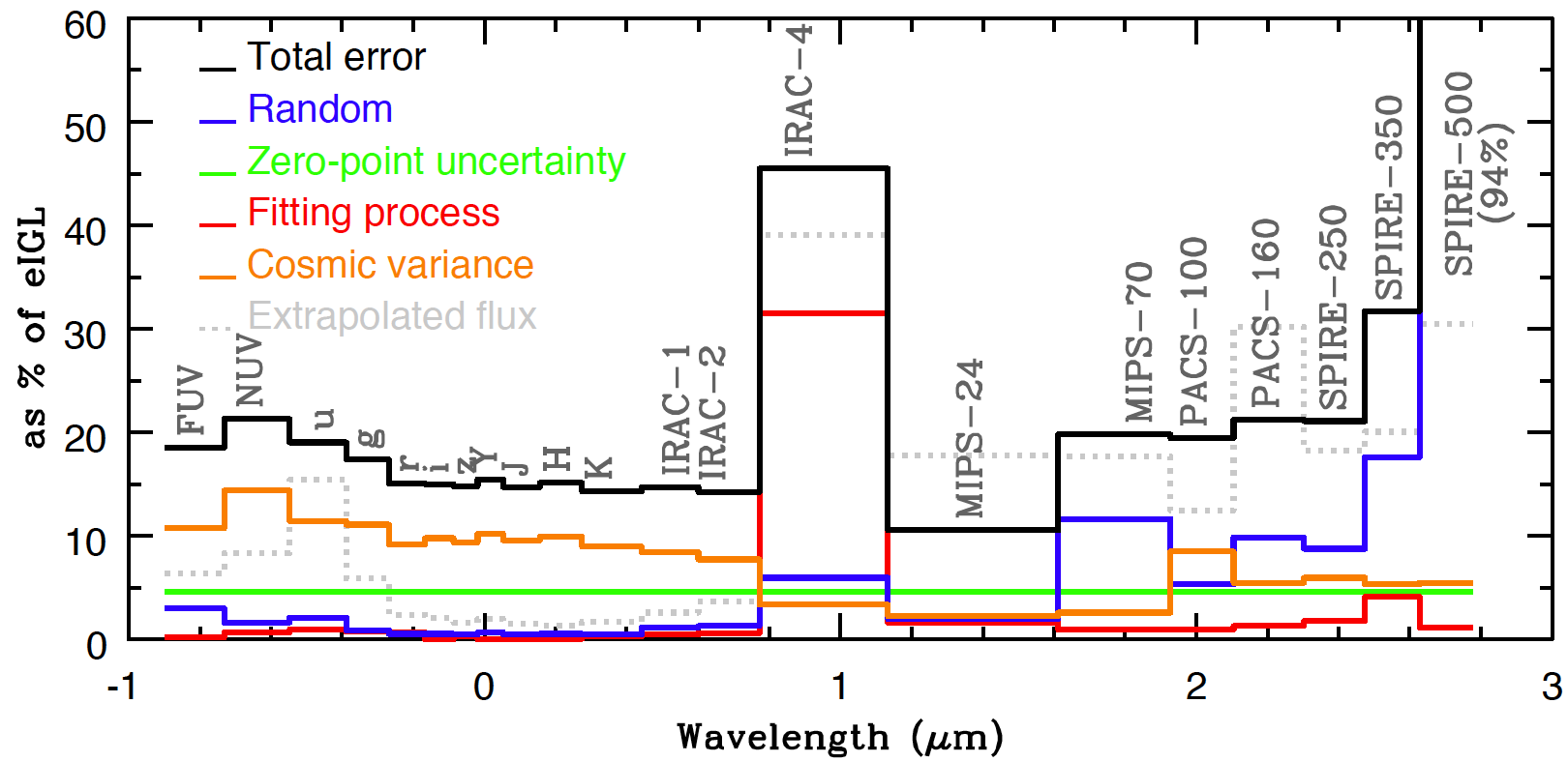
Figure 3.— The contribution of each of the individual errors as a percentage of the eIGL measurement as a function of wavelength (as indicated). The back line shows the total error which is mostly dominated by cosmic variance in the optical,near and mid-IR bands but by random errors in the far-IR bands.

3.3. Appropriate error estimation

There are a number of possible sources of error; in particular we consider those arriving from a systematic photometry error (zero-point shift, or background over/under estimation), the fitting process, those implied from the errors in the count data, and the possible impact of cosmic variance. We explore each of these in turn.

3.3.1 Photometric error

In most cases where we have multiple datasets we see that the counts agree within 0.05 mag, despite the potential for filter offsets due to small bandpass discrepancies. Generally, errors in absolute zero-points, particularly in HST data are expected to be $<0.01$—$0.02$ mag. However the process of sky-subtraction, object detection, and photometric measurement can lead to significant systematic variations. The easiest way to quantify the impact is to systematically shift all datasets by $\pm 0.05$ mag and re-derive our measurements. The value of $\pm 0.05$ mag comes from the amount required to align the various deep datasets, and is taken here to represent the systematic uncertainty in the entire photometric extraction process. This level of uncertainty should be considered conservative — surveys such as GAMA, for example typically quote errors of $\pm 0.03$ in photometric measurements — but high-$z$ galaxies are often asymmetric, and their photometry distorted by ambiguous deblends. Hence, a larger assumed error of $\pm 0.05$ mag seems plausible and prudent. Col. 6 of Table 2 shows the perturbation to the best-fit value if all data-points are systematically shifted by $\pm 0.05$ mag. Only for MIPS $24\mu$m does this error dominate (Fig. 3, green line).

3.3.2 Spline fitting error

The fitting process we adopt arbitrarily uses a 10-point spline-fit. This was judged to be the lowest number of spline points required to represent the data well. We repeat our analysis using an 8 or 12 point spline-fit and report the impact (Col. 7) on our best-fit value using these alternative representations, i.e., $|\Delta\rho_{L}|/2$. In all cases except for $IRAC$-$4$, where other issues have already been raised, the variation due to the fitting process is negligible (Fig. 3, red line).

3.3.3 Poisson error

To assess the error arising from the uncertainty in the individual data-points, we conduct 10,001 Monte-Carlo realizations where we randomly perturb each data-point by its permissible error, assuming the errors follow a Normal distribution. For each sequence of perturbations we re-fit the spline and extract the 16^thpercentile and the 84^th percentile values for the luminosity density. The uncertainty given in Col. 7 of Table 2 is then $|\Delta\rho_{L}|/2$. We see that this error becomes dominant for data longwards of MIPS $24\mu$m (Fig. 3, blue line).

3.3.4 Cosmic Variance error

Finally we assess the error introduced by cosmic variance (or sample variance), as discussed by Driver & Robotham (2010). For each dataset shown in Table. 1, we derive and assign a cosmic variance estimate based on equation 4 in Driver & Robotham (2010), using the appropriate areas of the various datasets and some assumption of the likely redshift range contributing to the counts (see Table. 1). We conduct 10,001 Monte-Carlo realizations, where we perturb each dataset by a random amount defined by its cosmic variance (assuming the CV offset can be drawn from a Normal distribution). We extract the 16^thpercentile and the 84^th percentiles, from which we derive an uncertainty, as, $|\Delta\rho_{L}|/2$. We see from Fig. 3 (orange line) that this error dominates for most of the UV, optical, near-IR, and mid-IR bands.

3.3.5 Combining errors

Combining random and systematic errors is not entirely straightforward, with some proponents advocating simply adding them while others adding in quadrature, or keeping the systematic and random errors separate. Here we take the most conservative approach of adding the errors linearly, but provide the individual errors in Table 2 for those wishing to combine them in other ways. The data points shown on subsequent figures are calculated according to $\Delta_{\rm Total}=\Delta_{\rm Col.6}+\Delta_{\rm Col.7}+\Delta_{\rm Col.8}+\Delta_{\rm Col.9}$

Fig. 3 shows the contribution of each of the individual errors to our eIGL measurements and highlights the transition from being dominated by cosmic variance error at shorter wavelengths to random errors at longer wavelengths. At one wavelength ($IRAC$-$4$), we note that the fitting error itself dominates because of the complex shape of the data. One clear consequence from Fig. 3 is that deep, wide data are essential to reduce this error component, which should be readily achievable in the optical and near-IR, with the upcoming Euclid and the Wide Field Infrared Space Telescope (WFIRST) space-missions. Assuming calibration errors can be minimised, there is the distinct possibility of obtaining eIGL measurements to better than 1% over the next decade.

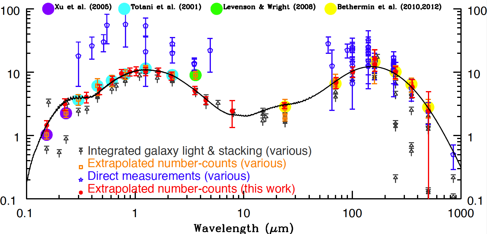
Figure 4.— Our measurement of the eIGL based on extrapolated number counts in each band compared to literature measurements taken from Dwek & Krennrich (2013). The black line depicts a phenomenological model from Andrews et al. (2016b). The blue data points are attempted direct measurements which requires accurate modeling of both the Milky Way and Zodiacal light.

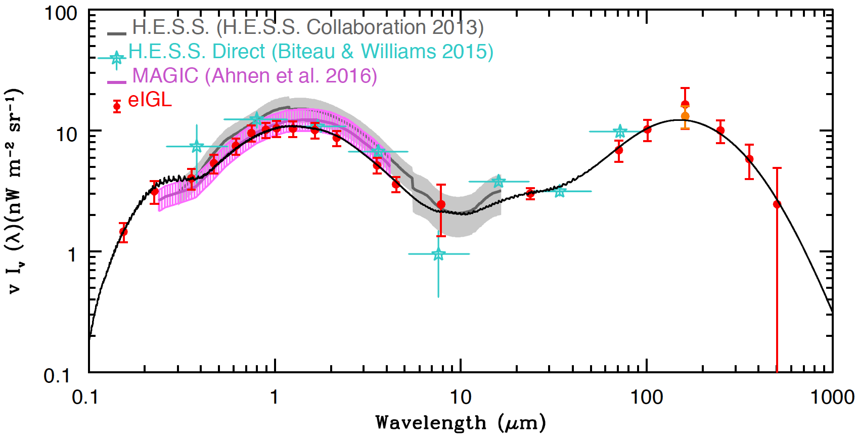
Figure 5.— Our measurements of the eIGL along with the model of Andrews et al. compared to the available VHE data from the H.E.S.S. and MAGIC Consortium (both of which use a pre-defined EBL model). The blue stars show the VHE constraint by Biteau & Williams (2015) which are independent of any pre-defined EBL model.

3.4. Comparison to previous EBL and eIGL measurements

Fig. 4 shows various IGL and EBL measurements as reported over the past few years. Most of the data comes from the comprehensive compilation by Dwek & Krennrich (2013) (see their tables 3, 4 & 5 for detailed references, although most appear here in the introduction and text), plus more recent measurements by Ashby et al. (2015). We colour code the data into three sets following Dwek & Krennrich: lower limits on the IGL (grey), IGL measurements based on various extrapolated number counts (orange); and direct measurements of the EBL via various methods (blue). Our new data is shown in red and appears consistent with most previous eIGL measurements. Within the eIGL data we only see one major discrepancy which is with the Levenson & Wright (2008) value in the $IRAC$-$1$ band. We find a significantly ($\times 2$) lower value. Levenson & Wright (2008) also combine galaxy count data from a number of sources and use two methods for deriving photometry, profile fitting and apertures. Both require significant corrections (upward shifts of $\sim 40$%). The value reported is from profile fitting, however, we note that their corrected aperture value is significantly lower ($5.9\pm 1.0$ nW m^-2 sr^-1), and consistent with our measurement ($5.2\pm 0.8$ nW m^-2 sr^-1). We argue that, as our 3.6$\mu$m measurement lies in between our $2.2\mu$m and $4.6\mu$m measurements, it is likely that the Levenson & Wright (2008) profile-fit value is biased high.

In the far-UV and near-UV, we recover higher measurements than those reported by Xu et al. (2005), although formally at the $1\sigma$ error-limits. However, this is nonetheless consistent with the data shown in Xu et al. (2005) (see their figure 1) where their number counts in both the far-UV and near-UV, to which their model is fitted, do appear to fall systematically below the comparison datasets. See also figure 6 of Voyer et al. (2011) which shows an offset between the data of Xu et al. (2005) and Hammer et al. (2010). Table. 2 of Voyer et al. (2011) reports eIGL measurements by Voyer et al. (2011) and Xu et al. (2005) as well as Gardner et al. (2000) and earlier studies. Our value agrees well — lies between — the two estimates provided by Voyer et al. (2011). In the near-UV our result is dependent on an entirely different dataset, namely F225W observations of the UVUDF. This base data is very different to the HST ACS SBC data of Voyer et al. (2011), and agrees closely to the much earlier HST STIS data of Gardner et al. (2000). We therefore conclude that the UV excess seen in our data against the model is supported by three distinct datasets and therefore likely real and significant.

In the far-IR, we see that our measurements mostly agree with those previously reported. The one obvious outlier is the PACS 160$\mu$m data, however we note (see Table 2) that a significant amount of flux is coming from the extrapolation. In particular the deepest data points from Magnelli et al. (2013) do include significant completeness corrections. If we re-fit using only data with completeness corrections at $<20$% (their filled data points on their figure 6), we recover a much more consistent value (see the second entry in Table 2 and orange data point on Fig. 4). We therefore elect to adopt this revised data point as the more robust estimate.

Most apparent from Fig. 4 is the discrepancy in the optical to near-IR between all the eIGL data (including our own), and the direct measurements. This is in stark contrast to the far-IR where the eIGL and EBL measurements agree within the specific errors. In the case of the far-IR, the agreement is reassuring, and the much smaller error bars on the eIGL measurements suggest that the eIGL route is the more robust. Why then do we see such a discrepancy in the optical? The model curve (black) shows the energy evolution model reported in Andrews et al. (2016b), which agrees closely with the eIGL data. Both the model and the general consensus in the far-IR would therefore suggest that the error may lie in the direct measurements, some of which do concur with the eIGL estimates. It is worth noting that direct measurements rely on a robust subtraction of the foreground light of which there are two dominant sources: the Milky Way stellar population and Zodiacal light (Hauser & Dwek, 2001; Mattila, 2006). That the discrepancy is most apparent at a wavelength comparable to the peak in the solar spectrum also suggests that one or both of these foregrounds is the source of the problem, and that either the Milky Way model or the Zodiacal model have been underestimated. One indication for the latter over the former is the reanalysis of data taken between 1972—1974 at 0.44$\mu$m and 0.65$\mu$m by the Pioneer 10/11 spacecraft (Matsuoka et al., 2011). During that period the spacecraft were approximately 4.66AU away from the Sun where the Zodiacal light contribution should be negligible. Matsuoka found significantly lower EBL measurements that are in agreement with our eIGL values. We advocate that given this information, it might be useful to adopt the eIGL as the de facto measurements of the EBL, and use these to help improve the Zodiacal light and inner Solar System dust model.

3.5. Comparison to very high energy data

Fig. 5 shows the comparison of our eIGL data to three VHE datasets (as indicated). The agreement is much better than with the direct estimates, and provides additional independent evidence that the direct estimates may be in error. Note that the H.E.S.S. and MAGIC datasets each adopt a pre-defined EBL model and solve for the normalisation, hence the slight shape discrepancy between the VHE and eIGL data is of no significance. Formally, the datasets overlap within the 1$\sigma$ errors, although the error range of the VHE data is fairly broad ($\times 2$). As discussed in the introduction, the VHE data also comes with some caveats, in particular the assumption of the intrinsic shape of the Blazar spectra(um), the possibility of other interactions, e.g., with the intergalactic magnetic field or with PeV cascades. Nevertheless, the agreement is extremely encouraging and taken at face value suggests that our eIGL measurements are close to the underlying EBL values.

3.6. Potential sources of missing light

Before equating our eIGL measurement to the EBL we should first acknowledge, in particular, the possible contributions from the low surface brightness Universe: that from intra-cluster and intra-group light (Zwicky, 1951), also referred to as Intra-Halo Light or IHL (Zemcov et al., 2014); and that from the epoch of reionisation (Cooray et al., 2012).

3.6.1 Low surface brightness galaxies

The space-density of low surface brightness galaxies is currently poorly constrained, however observations in the local group suggest that the luminosity density is very much dominated by the Milky Way and Andromeda. This picture is generally supported by our own estimates of the low surface brightness population from the HST HDF (Driver, 1999) and the Millennium Galaxy Catalogue (see Liske et al., 2003; Driver et al., 2005). Both studies explored the low surface brightness Universe and, while finding numerous new systems, they ultimately contribute only small amounts of additional light ($<20$%; Driver, 1999). Studies of rich clusters have also been very successful at finding low surface brightness systems (e.g., Davies et al., 2015; van Dokkum et al., 2015), yet not in sufficient quantities to significantly affect the total luminosity density, e.g., the thousand new galaxies found in the Coma cluster by Koda et al. (2015) collectively add up to just one extra L^∗ galaxy.

Two final arguments can be made for a minimal amount of missing light from low surface brightness galaxies based on the number-count and IGL data itself. Firstly, as each survey would have distinct surface brightness cutoffs, any large population would be truncated at different surface brightness levels leading to stark mismatches between the distinct surveys. That the surveys overlap so well is a strong argument for any missing population being relatively modest in terms of their luminosity density. Secondly, any missing population of galaxies will contain both optical emission from the starlight, and dust emission from reprocessed starlight. Hence the consistency between the far-IR EBL and eIGL can provide a constraint. To assess this we compare our values of the eIGL to the direct EBL measurements of Fixsen et al. (1998), and derive (eIGL/EBL) ratios of 0.96, 0.97, 1.05 and 1.03 in 160, 250, 350 and 500$\mu$m bands for an average of 1.01, i.e., on average 100% of the direct EBL is “resolved” by our eIGL measurements.

This therefore only gives no room for an upward adjustment for missing “dusty” galaxies. However we do acknowledge that the errors in both our data and the Fixsen data are significant (typically 40% per band), and hence this close agreement must be somewhat coincidental. Folding in the errors there is potentially room for an $\sim 19\%$ upward adjustment, i.e., $40\%/\sqrt{4}$, before our eIGL exceeds the Fixsen EBL measurements by their reported 1$\sigma$ errors. Of course this argument assumes that the dust properties of low surface brightness galaxies are consistent with those of normal spiral galaxies, which may not be the case. A similar conclusion, with regards missing galaxy light, was also reached by Totani et al. (2001), who specifically explored the potential impact of surface brightness selection in deep Subaru number counts, and concluded that any impact from missing low surface brightness galaxies, via number-count modeling, was $<20$% in the $BVIJL$ bands. Our range of 20% is comparable and hence we can adopt a possible 0—20% upward adjustment range for missing low surface brightness galaxies.

3.6.2 Intra-cluster and intra-group light

The case for the intra-cluster light is slightly less clear-cut. Mihos et al. (2005) shows spectacular images of nearby systems, including Virgo, which typically contain between 10-20% of the light in a diffuse component. In the Frontiers’ cluster A2744, Montes & Trujillo (2014) find that the ICL makes up only 6% of the stellar mass. Similarly, the study by Presotto et al. (2014) also finds a relatively modest amount of mass (8%) in the CLASH-VLT cluster MACS J1206.2-0847. Earlier studies of Coma, perhaps the most studied system, found significantly more diffuse light, extending up to almost 50% (Bernstein et al., 1995), and simulations by Rudick et al. (2011) suggest the ICL might contain anywhere from 10-40% of a rich cluster’s total luminosity. Hence, studies of the ICL could be used to argue for an upward adjustment of the optical-only light of between 10-50%. However it is important to remember that rich clusters, such as Coma, the Frontier’s, and CLASH clusters are exceedingly rare (Eke et al., 2005), with less than 2% of the integrated galaxy light coming from $>10^{14.5}$M_⊙ haloes (see Eke et al., 2005 and Driver et al., 2016b).

In the absence of quality data, intuition can lead one in both directions, as the fraction of diffuse light is likely to be a function of the halo velocity dispersion, and the galaxy-galaxy interaction velocity, duration, and frequency. Certainly evidence from the local group suggests a fairly modest contribution, with the Magellanic stream representing the only significant known source of diffuse light. Furthermore the deep study of M96 (Leo I group) by Watkins et al. (2014), failed to identify any significant intra-group light to limits of 30.1 mag/sq arcsec.

Intra-halo light will only affect the optical bands as it is dust free due to the UV flux pervading the ICM destroying any dust particles. We can therefore gauge the possible level by comparing our eIGL $g$ band measurement to the EBL. As mentioned earlier, because of uncertainties in the Zodiacal light model we cannot use most of the direct estimates, however we can use the values provided by Matsuoka et al. (2011) obtained from Pioneer 10/11. Using these we find eIGL/EBL ratios of $0.68\pm 0.23$ and $0.97\pm 0.43$ in the $g$ and $r$ bands respectively (with the errors dominated by the uncertainty in the Pioneer estimates). The errors are large but suggest that the contribution from the IHL (which can only be positive) lies in the range 3-32% but with a possible extreme upper limit of $\sim$35% (i.e., $\frac{(0.68-0.23)+(0.97-0.43)}{2}/\sqrt{2}$) upward correction of the optical and near-IR data (in-line with our earlier discussion of the ICL).

3.6.3 Reionisation

Reionisation could potentially provide an additional diffuse photon field in the near-IR range, i.e., where Ly$\alpha$ is redshifted longwards of $1\mu$m. Recent modeling by Cooray et al. (2012) suggests the flux of reionisation today might be in the range 0.1 - 0.3 nW m^-2 sr^-1 at $\sim 1.1\mu$m, i.e. a 3% effect. This is well below our quoted errors and so reionisation is unlikely to significantly impact upon our measurements. However, it is worth noting that the reionisation models are uncertain, and a more rigid upper-limit of $\sim 2$ nW m^-2 sr^-1 at $1\mu$m was set by Madau & Silk (2005), based on arguments which related to the production of excessive metals if the reionising flux was any stronger. This latter level is plausibly detectable and could cause our eIGL to underestimate the EBL by $\sim 20$% in the near-IR. Hence comparison of the near-IR eIGL to direct EBL measurements could conceivably detect the reionisation field.

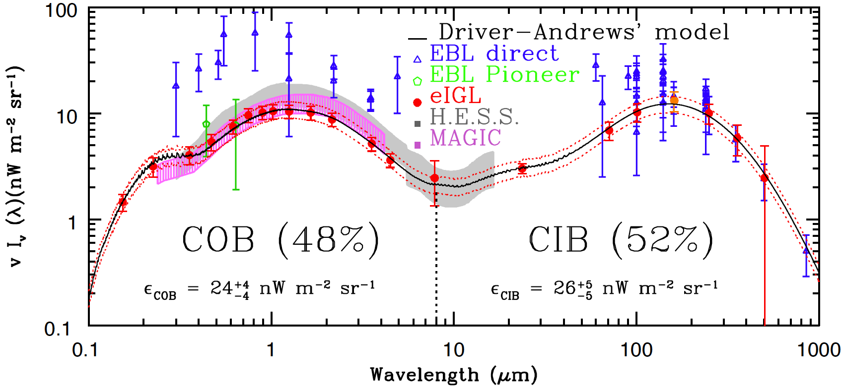
Figure 6.— Our derived eIGL data (red points), compared to terrestrial and near Solar System direct measurements (blue triangles), and the direct estimates from the Pioneer spacecraft at $>4.5AU$ (green circles). Also shown is the modified Driver-Andrews’ model (black line) and the error bounds (red dashed lines) adopted for determining the uncertainty in the integrated COB and CIB measurements (as shown).

3.6.4 eIGL $\rightarrow$ EBL

The eIGL and the EBL are, from the discussion above, slightly different entities where the eIGL represents the sum of all radiation from bound galaxies while the EBL includes, in addition, diffuse light from the IHL and the epoch of reionisation. However we have estimated in comparison to the available direct EBL estimates that the eIGL should match the EBL to within 0—35% in UV-optical-near-IR bandpasses and 0—20% in far-IR bandpasses. These numbers are also consistent with the discrepancy between our eIGL measurements and the indirect VHE measurements. Specifically in $J$ band we find an eIGL value of $10.38\pm 1.52$ while the H.E.S.S. Collaboration find a range for the EBL of 18.5—-11.5 and the MAGIC team a range of 14.8—9.8. Formally our values are consistent. Again the means our value is low by 45% and 18% but with no ($<1\sigma$ significance). The take home message is more that the eIGL and VHE EBL data show promising consistency, and if the errors in both can be reduced in significance comparisons could potentially provide very interesting constraints on the diffuse Universe.

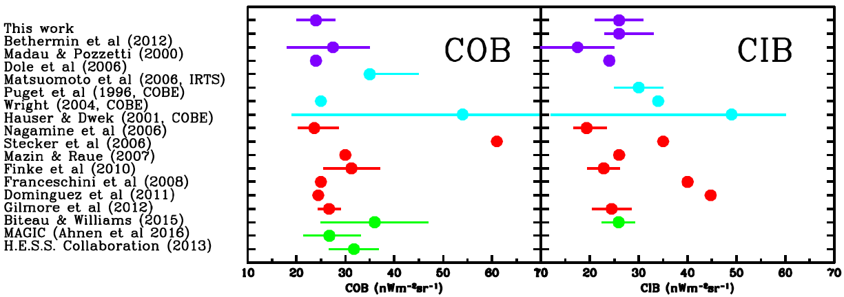
Figure 7.— A selection of available COB and CIB measurements which includes eIGL estimates (mauve), direct measurements (cyan), numerical models (red), and VHE results (green). Error ranges are shown if provided.

3.7. The integrated energy of the COB and CIB

Finally, to determine the COB and CIB from our data we need to identify an appropriate fitting function. In this case the most straightforward option is to adopt a model which closely matches the data. Shown on Figs. 4 & 5 is a model prediction from Andrews et al. (2016a) which is based on an update to the two-component phenomenological model of Driver et al. (2013). In this model, we link spheroid formation to AGN activity, and adopted the axiom that spheroid formation dominates at high-redshift. The variation of AGN activity with redshift provides the shape, and the cosmic star-formation history provides the normalisation, for the star-formation history of spheroids only. The star-formation history of discs is then the discrepancy between the total cosmic star-formation history, and the spheroid star-formation history. With the star-formation history of spheroids and discs defined, we use a stellar population synthesis code and some underlying assumption of the metallicity evolution (linear increase with star-formation), to predict the cosmic spectral energy distribution at any epoch, and compare to the available data at $z<0.1$ (see Driver et al., 2013 for full details). The model has now been developed to included obscured and unobscured AGN, bolstering the UV flux, as well as dust reprocessing and the model will be presented in detail in Andrews et al. (2016b).

In Fig. 6 we again show our eIGL data compared to our adopted model which provides a reasonable fit across the full wavelength range shown. We perform a standard error-weight $\chi^{2}$-minimisation of the model against the data to determine the optimal normalisation and the $1\sigma$ error ranges on this normalisation. Note that we fit the EBL data to the COB and CIB separately, and while the overall normalisations agree the recovered $1\sigma$ errors are slightly broader for the CIB data (reflecting the large associated errors). We now integrate the EBL model using the $R$ (integrate) function from $0.1$ to 8$\mu$m and $8$ to 1000$\mu$m to obtain the total energy contained within the COB and CIB. We find values of $24^{+4}_{-4}$ nW m^-2 sr^-1 and $26^{+5}_{-5}$ nW m^-2 sr^-1 respectively, essentially a 48:52% split.

Fig. 7 shows some of the COB and CIB measurements reported in the literature based on either integrated galaxy counts (mauve), direct estimates (cyan), numerical models (red) or VHE data (green). Our values agree well with previous eIGL estimates, and in particular with the most recent CIB measurement of Béthermin et al. (2012) ($27^{+7}_{-3}$ nW m^-2 sr^-1). This should not be particularly surprising as our CIB fits lean heavily on the Béthermin source-count data, however the consistency in the measurement and errors is reassuring. In general we do see a trend, that the eIGL values are the lowest, the direct estimates the highest, and that the VHE data is closer, but slightly higher, than the eIGL estimates. This does imply that there may indeed be an additional diffuse component (photon field) at the $\sim 20$% level. As discussed above this could plausibly be due to some combination of low surface brightness galaxies, intra-halo light, and or any diffuse radiation from reionisation. At the moment the errors are to broad to draw any firm conclusion however, as observations improve in wide area imaging (Euclid, WFIRST, LSST), and in VHE capabilities, there is a strong possibility of placing a meaningful constraint on this diffuse component. In our analysis the dominant errors in the COB, at least, are very much due to cosmic variance which are currently at the 5-10% level but can conceivably be reduced to below 1% in the near future. The normalised EBL model is available in machine readable format from the ApJ online edition.

4. Summary

We have brought together a number of panchromatic datasets (GAMA, COSMOS/G10, HST ERS, UVUDF and other mid and far-IR data) to produce galaxy number counts which typically span over 10 magnitudes and from the far-UV to the far-IR. Having homogenized the data, we apply a consistent methodology to derive an integrated galaxy light and an extrapolated galaxy-count light (eIGL) measurement. The method avoids traditional galaxy number-count models and, as all datasets are bounded in terms of the contribution to the IGL, are simply fit with a 10-point spline. Integrating the spline with or without extrapolation then leads to a complete set of IGL measurements from the far-UV to far-IR. Our error analysis includes four key components: a systematic photometry and/or zero-point offset of $\pm 0.05$ mag in all datasets, a re-fit based on 8 or 12 point splines, 10,001 Monte-Carlo realizations of the random errors, and 10,001 Monte-Carlo realizations of the cosmic variance estimates. We combine the errors linearly to produce our final eIGL measurements, which are accurate to 2-30% depending on bandpass.

In comparison to previous data we generally agree with previous IGL measurements, agree with direct measurements in the far-IR, but disagree with direct measurements in the optical (see Fig. 4, blue data points). We question whether the Milky Way or Zodiacal light model requires revisiting for the direct optical and near-IR measurements. In particular we note (see Fig. 6) that the direct estimates from Pioneer agree well with our eIGL estimates as do the constraints from very high energy experiments, suggesting a possible issue with the inner Solar System dust model.

We briefly acknowledge that the eIGL measurements could potentially miss light from low surface brightness systems (0-20%) and intra cluster/group light (0-35%). Insofar as studies exists evidence suggests such emissions are likely small ($<20$%) and within our quoted errors. However studies to further constrain both the space-density of low surface brightness galaxies and the intra-halo light would clearly be pertinent.

Finally we overlay the two-component model of Driver et al. (2013), which now includes AGN (Andrews et al., 2016b) and find that we can explain the eIGL distribution rather trivially in terms of a spheroid/AGN formation phase ($z>1.5$), followed by disc formation ($z<1.5$). Using a slightly modified version of the model as a fitting function we find that the COB and CIB contain $24^{+4}_{-4}$ nW m^-2 sr^-1 and $26^{+5}_{-5}$ nW m^-2 sr^-1 respectively, essentially a 48:52% split.

Over the coming years with the advent of wide-field space-based imaging, and in particular Euclid and WFIRST, we note the great potential to constraint the UV, optical and near-IR optical backgrounds to below 1%.

Appendix A Additional wavebands

Figures A1 to A6 shows the number count and luminosity density figures for those datasets not shown in Fig. 2, i.e., FUV/NUV, ugi, $ZYJHK$, $IRAC$-2&4, MIPS24, PACS70/100/160 and SPIRE 350/500. The description of the lines, labels and key is as for Fig. 2.

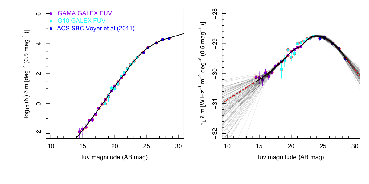
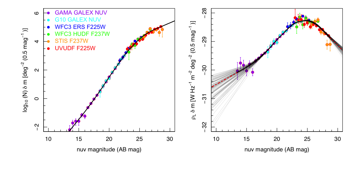
Figure A1.— As for Fig. 2 but for FUV, NUV and $u$ bands.

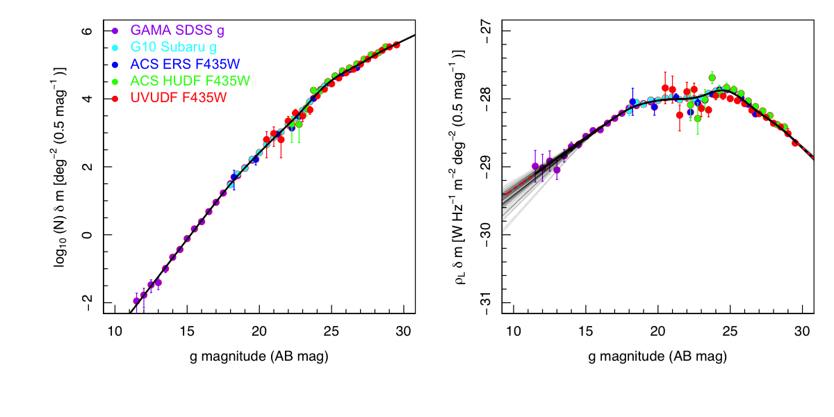
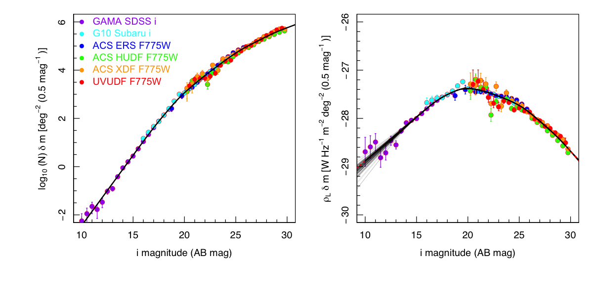
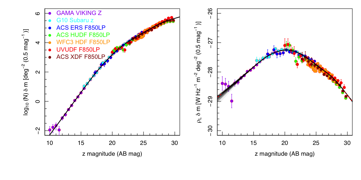
Figure A2.— As for Fig. 2 but for $g$, $i$ and $z$ bands.

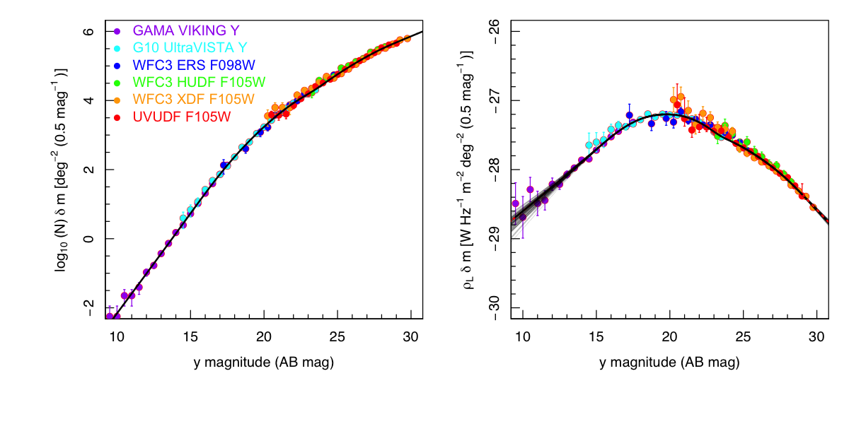
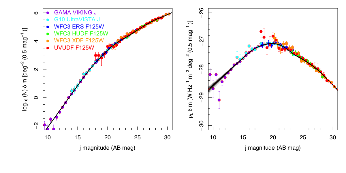
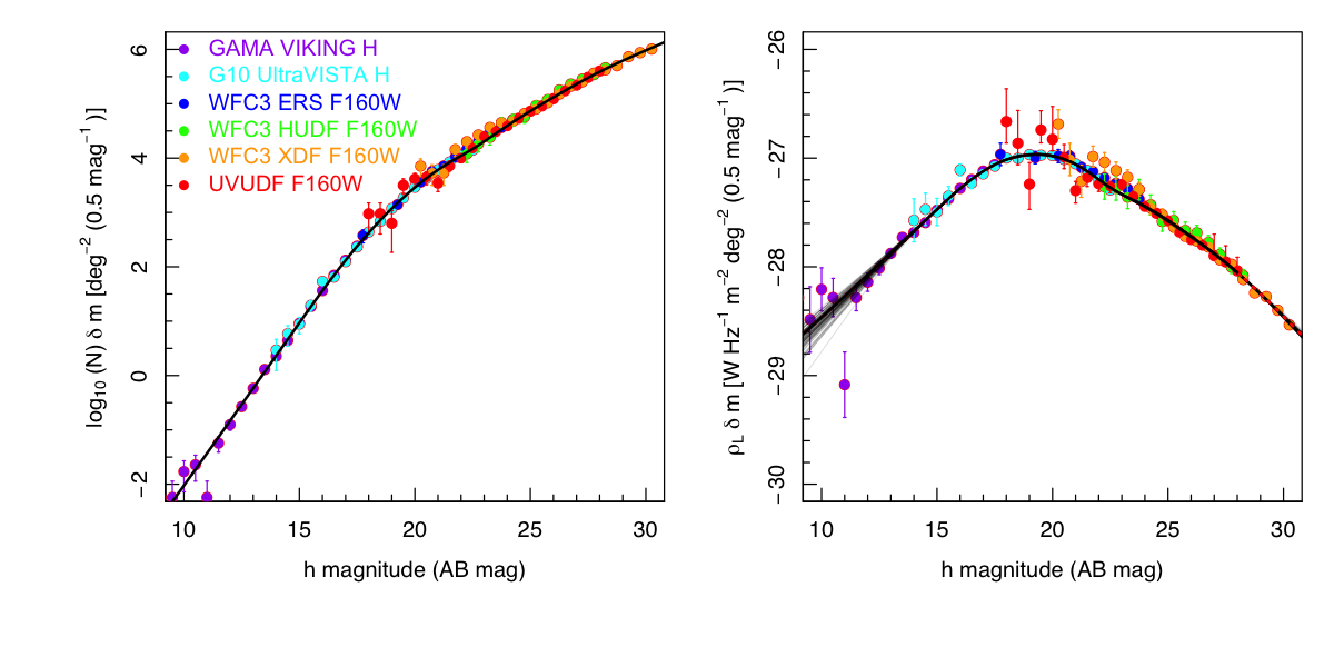
Figure A3.— As for Fig. 2 but for $Y$, $J$ and $H$ bands.

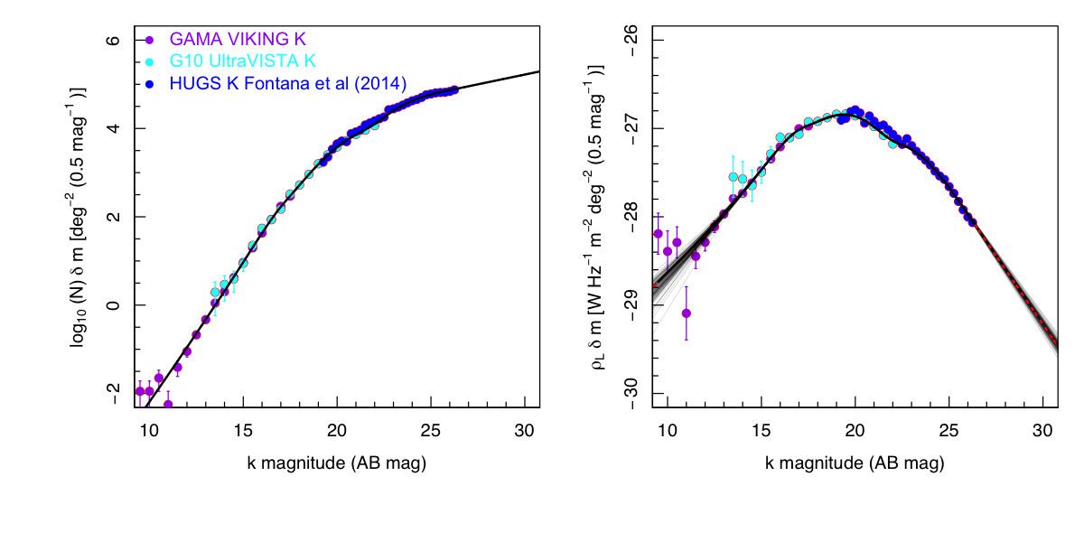
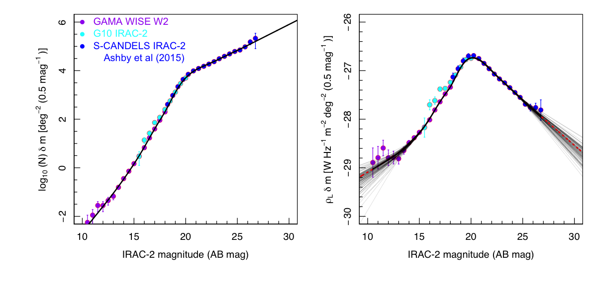
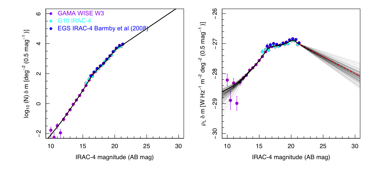
Figure A4.— As for Fig. 2 but for $K$, $IRAC$-$2$ and $IRAC$-$4$ bands.

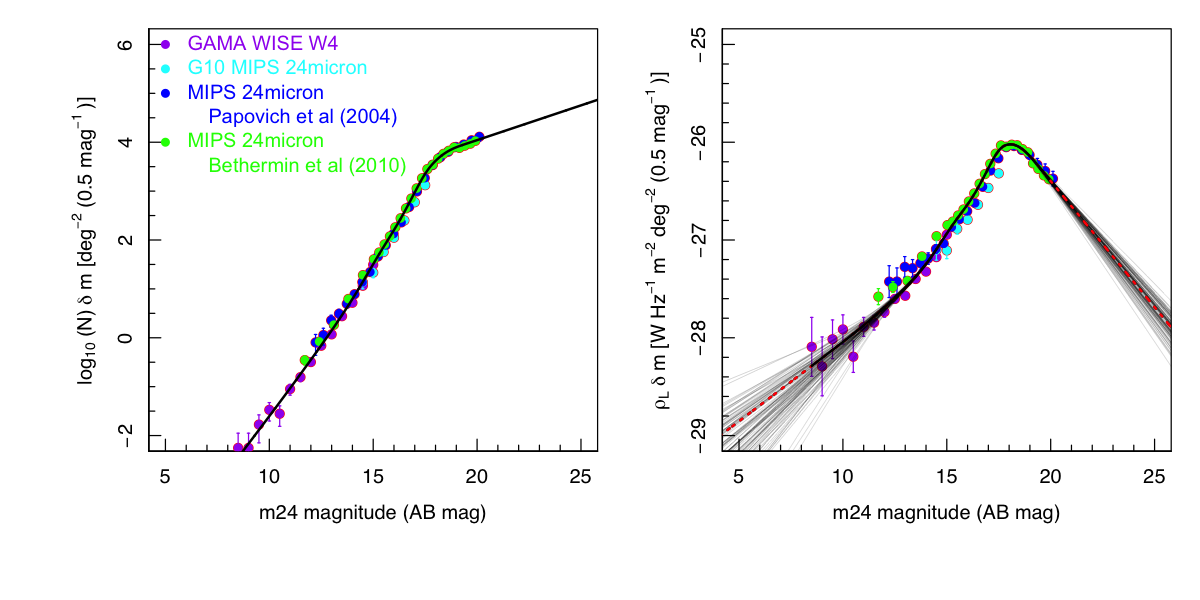
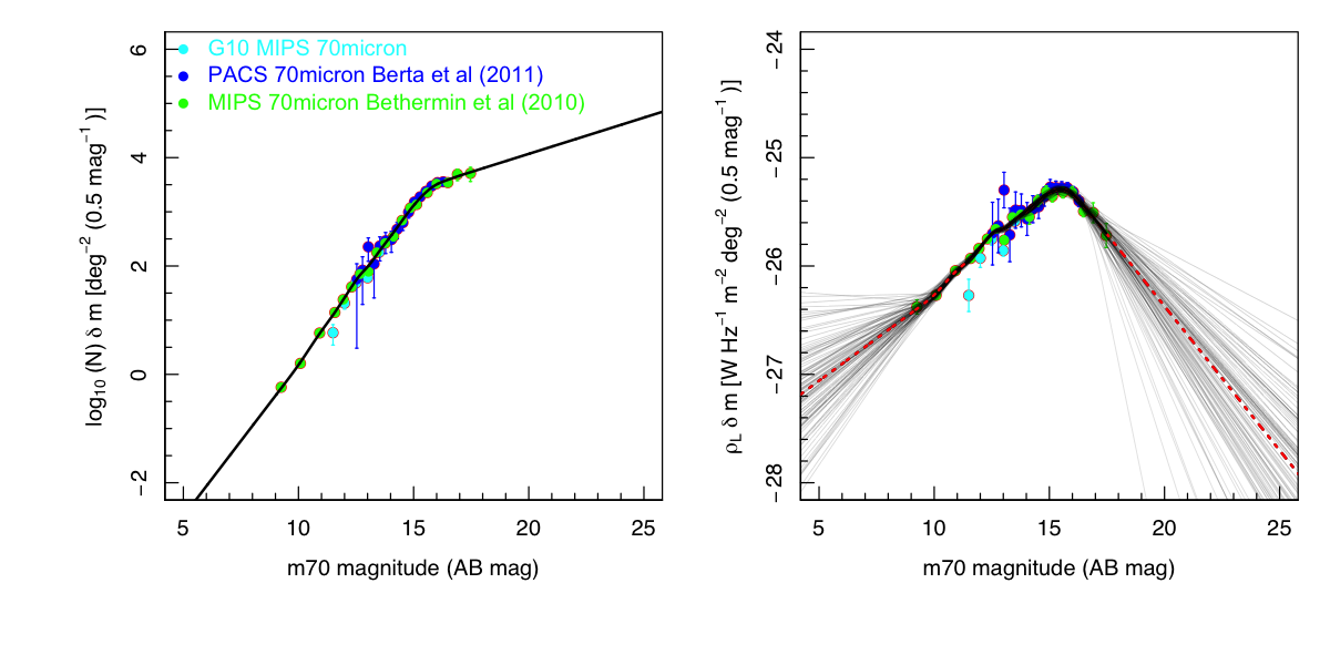
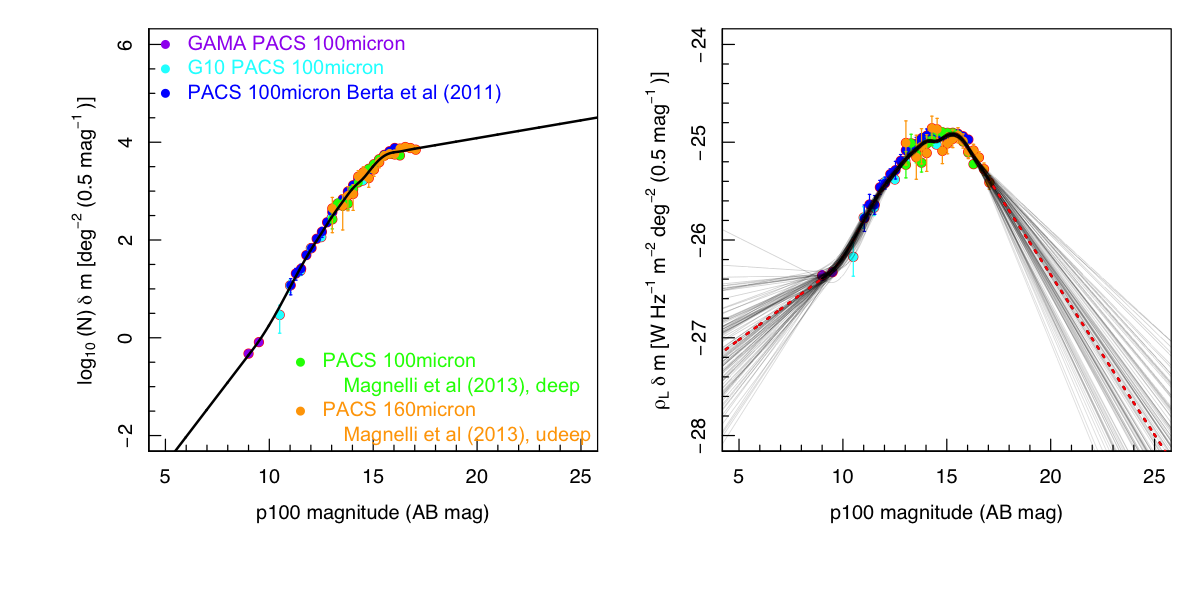
Figure A5.— As for Fig. 2 but for $24\mu$m, MIPS/PACS $70\mu$m and PACS $100\mu$m bands.

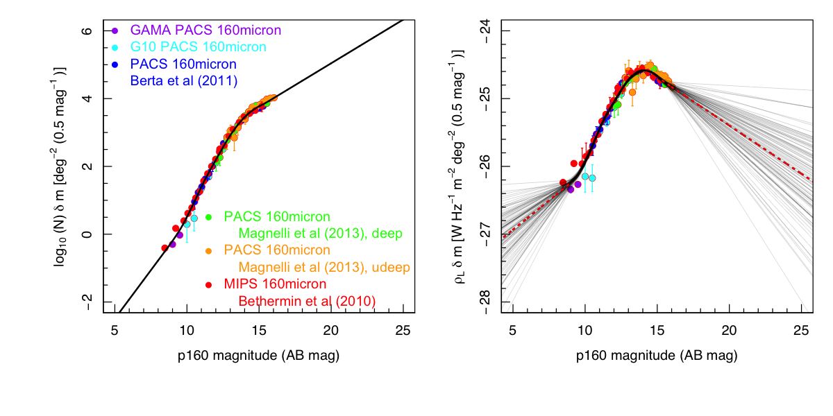
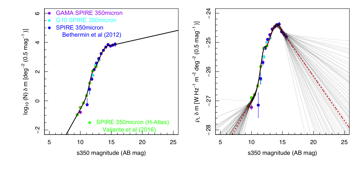
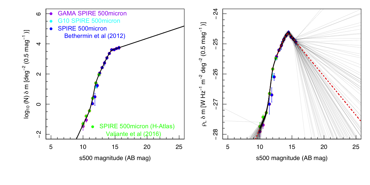
Figure A6.— As for Fig. 2 but for PACS $160\mu$m, SPIRE $350\mu$m and SPIRE $500\mu$m bands.

References

- Aharonian et al. (2006) Aharonian, F., Akhperjanian, A. G., Bazer-Bachi, A. R., et al. 2006, Nature, 440, 1018
- Ahnen et al. (2016) Ahnen, M. L., Ansoldi, S., Antonelli, L. A., et al. 2016, arXiv:1602.05239
- Alexander et al. (2005) Alexander, D. M., Bauer, F. E., Chapman, S. C., et al. 2005, ApJ, 632, 736
- Andrews et al. (2016a) Andrews, S. K., et al. 2016a, MNRAS, submitted
- Andrews et al. (2016b) Andrews, S. K., et al. 2016b, MNRAS, in prep.
- Ashby et al. (2015) Ashby, M. L. N., Willner, S. P., Fazio, G. G., et al. 2015, ApJS, 218, 33
- Barmby et al. (2008) Barmby, P., Huang, J.-S., Ashby, M. L. N., et al. 2008, ApJS, 177, 431
- Bernstein et al. (1995) Bernstein, G. M., Nichol, R. C., Tyson, J. A., Ulmer, M. P., & Wittman, D. 1995, AJ, 110, 1507
- Bernstein (2007) Bernstein, R. A. 2007, ApJ, 666, 663
- Bernstein et al. (2002) Bernstein, R. A., Freedman, W. L., & Madore, B. F. 2002, ApJ, 571, 56
- Berta et al. (2011) Berta, S., Magnelli, B., Nordon, R., et al. 2011, A&A, 532, A49
- Bertin & Arnouts (1996) Bertin, E., Arnouts, S., 1996, A&AS, 117, 393
- Béthermin et al. (2010) Béthermin, M., Dole, H., Beelen, A., & Aussel, H. 2010, A&A, 512, A78
- Béthermin et al. (2012) Béthermin, M., Le Floc’h, E., Ilbert, O., et al. 2012, A&A, 542, A58
- Biteau & Williams (2015) Biteau, J., & Williams, D. A. 2015, ApJ, 812, 60
- Cambrésy et al. (2001) Cambrésy, L., Reach, W. T., Beichman, C. A., & Jarrett, T. H. 2001, ApJ, 555, 563
- Capak et al. (2007) Capak, P., Aussel, H., Ajiki, M., et al. 2007, ApJS, 172, 99
- Chabrier (2003) Chabrier, G. 2003, PASP, 115, 763
- Cluver et al. (2014) Cluver, M. E., Jarrett, T. H., Hopkins, A. M., et al. 2014, ApJ, 782, 90
- Cooray et al. (2012) Cooray, A., Gong, Y., Smidt, J., & Santos, M. G. 2012, ApJ, 756, 92
- Dale et al. (2014) Dale, D. A., Helou, G., Magdis, G. E., et al. 2014, ApJ, 784, 83
- de Oliveira-Costa et al. (2008) de Oliveira-Costa, A., Tegmark, M., Gaensler, B. M., et al. 2008, MNRAS, 388, 247
- Dole et al. (2006) Dole, H., Lagache, G., Puget, J.-L., et al. 2006, A&A, 451, 417
- Davies et al. (2015) Davies, L. J. M., Driver, S. P., Robotham, A. S. G., et al. 2015, MNRAS, 447, 1014
- Davies et al. (2016) Davies, J. I., Davies, L. J. M., & Keenan, O. C. 2016, MNRAS, 456, 1607
- Domínguez et al. (2011) Domínguez, A., Primack, J. R., Rosario, D. J., et al. 2011, MNRAS, 410, 2556
- Driver et al. (2016a) Driver, S. P., Wright, A. H., Andrews, S. K., et al. 2016, MNRAS, 455, 3911
- Driver et al. (2013) Driver, S. P., Robotham, A. S. G., Bland-Hawthorn, J., et al. 2013, MNRAS, 430, 2622
- Driver et al. (2012) Driver, S. P., Robotham, A. S. G., Kelvin, L., et al. 2012, MNRAS, 427, 3244
- Driver et al. (2011) Driver, S. P., Hill, D. T., Kelvin, L. S., et al. 2011, MNRAS, 413, 971
- Driver & Robotham (2010) Driver, S. P., & Robotham, A. S. G. 2010, MNRAS, 407, 2131
- Driver et al. (2008) Driver, S. P., Popescu, C. C., Tuffs, R. J., et al. 2008, ApJ, 678, L101
- Driver et al. (2007) Driver, S. P., Popescu, C. C., Tuffs, R. J., et al. 2007, MNRAS, 379, 1022
- Driver (1999) Driver, S. P. 1999, ApJ, 526, L69
- Driver et al. (2005) Driver, S. P., Liske, J., Cross, N. J. G., De Propris, R., & Allen, P. D. 2005, MNRAS, 360, 81
- Driver et al. (2016b) Driver, S.P., et al. 2016, MNRAS, in prep.
- Dunne et al. (2011) Dunne, L., Gomez, H. L., da Cunha, E., et al. 2011, MNRAS, 417, 1510
- Dwek & Krennrich (2013) Dwek, E., & Krennrich, F. 2013, Astroparticle Physics, 43, 112
- Dwek & Arendt (1998) Dwek, E., & Arendt, R. G. 1998, ApJ, 508, L9
- Dwek et al. (1998) Dwek, E., Arendt, R. G., Hauser, M. G., et al. 1998, ApJ, 508, 106
- Eales et al. (2010) Eales, S., Dunne, L., Clements, D., et al. 2010, PASP, 122, 499
- Eke et al. (2005) Eke, V. R., Baugh, C. M., Cole, S., et al. 2005, MNRAS, 362, 1233
- Finke et al. (2010) Finke, J. D., Razzaque, S., & Dermer, C. D. 2010, ApJ, 712, 238
- Fixsen et al. (1998) Fixsen, D. J., Dwek, E., Mather, J. C., Bennett, C. L., & Shafer, R. A. 1998, ApJ, 508, 123
- Fontana et al. (2014) Fontana, A., Dunlop, J. S., Paris, D., et al. 2014, A&A, 570, A11
- Franceschini et al. (2008) Franceschini, A., Rodighiero, G., & Vaccari, M. 2008, A&A, 487, 837
- Frayer et al. (2009) Frayer, D. T., Sanders, D. B., Surace, J. A., et al. 2009, AJ, 138, 1261
- Gardner et al. (2000) Gardner, J. P., Brown, T. M., & Ferguson, H. C. 2000, ApJ, 542, L79
- Gilmore et al. (2012) Gilmore, R. C., Somerville, R. S., Primack, J. R., & Domínguez, A. 2012, MNRAS, 422, 3189
- Grazian et al. (2009) Grazian, A., Menci, N., Giallongo, E., et al. 2009, A&A, 505, 1041
- H.E.S.S. Collaboration et al. (2013) H.E.S.S. Collaboration, Abramowski, A., Acero, F., et al. 2013, A&A, 550, A4
- Hammer et al. (2010) Hammer, D., Verdoes Kleijn, G., Hoyos, C., et al. 2010, ApJS, 191, 143
- Hauser et al. (1998) Hauser, M. G., Arendt, R. G., Kelsall, T., et al. 1998, ApJ, 508, 25
- Hauser & Dwek (2001) Hauser, M. G., & Dwek, E. 2001, ARA&A, 39, 249
- Hill et al. (2011) Hill, D. T., Kelvin, L. S., Driver, S. P., et al. 2011, MNRAS, 412, 765
- Hopkins et al. (2013) Hopkins, A. M., Driver, S. P., Brough, S., et al. 2013, MNRAS, 430, 2047
- Hopwood et al. (2010) Hopwood, R., Serjeant, S., Negrello, M., et al. 2010, ApJ, 716, L45
- Inoue et al. (2013) Inoue, Y., Inoue, S., Kobayashi, M. A. R., et al. 2013, ApJ, 768, 197
- Jarrett et al. (2011) Jarrett, T. H., Cohen, M., Masci, F., et al. 2011, ApJ, 735, 112
- Jauzac et al. (2011) Jauzac, M., Dole, H., Le Floc’h, E., et al. 2011, A&A, 525, A52
- Kashlinsky (2006) Kashlinsky, A. 2006, New A Rev., 50, 208
- Keenan et al. (2010) Keenan, R. C., Barger, A. J., Cowie, L. L., & Wang, W.-H. 2010, ApJ, 723, 40
- Khaire & Srianand (2015) Khaire, V., & Srianand, R. 2015, ApJ, 805, 33
- Koda et al. (2015) Koda, J., Yagi, M., Yamanoi, H., & Komiyama, Y. 2015, ApJ, 807, L2
- Krick et al. (2009) Krick, J. E., Surace, J. A., Thompson, D., et al. 2009, ApJS, 185, 85
- Lagache et al. (2005) Lagache, G., Puget, J.-L., & Dole, H. 2005, ARA&A, 43, 727
- Lagache et al. (1999) Lagache, G., Abergel, A., Boulanger, F., Désert, F. X., & Puget, J.-L. 1999, A&A, 344, 322
- Levenson & Wright (2008) Levenson, L. R., & Wright, E. L. 2008, ApJ, 683, 585
- Levenson et al. (2010) Levenson, L., Marsden, G., Zemcov, M., et al. 2010, MNRAS, 409, 83
- Lilly et al. (2007) Lilly, S. J., Le Fèvre, O., Renzini, A., et al. 2007, ApJS, 172, 70
- Liske et al. (2003) Liske, J., Lemon, D. J., Driver, S. P., Cross, N. J. G., & Couch, W. J. 2003, MNRAS, 344, 307
- Liske et al. (2015) Liske, J., Baldry, I. K., Driver, S. P., et al. 2015, MNRAS, 452, 2087
- Lutz et al. (2011) Lutz, D., Poglitsch, A., Altieri, B., et al. 2011, A&A, 532, A90
- Madau & Pozzetti (2000) Madau, P., & Pozzetti, L. 2000, MNRAS, 312, L9
- Madau & Silk (2005) Madau, P., & Silk, J. 2005, MNRAS, 359, L37
- Magnelli et al. (2013) Magnelli, B., Popesso, P., Berta, S., et al. 2013, A&A, 553, A132
- Mattila (2006) Mattila, K. 2006, MNRAS, 372, 1253
- Matsumoto et al. (2015) Matsumoto, T., Kim, M. G., Pyo, J., & Tsumura, K. 2015, ApJ, 807, 57
- Matsumoto et al. (2011) Matsumoto, T., Seo, H. J., Jeong, W.-S., et al. 2011, ApJ, 742, 124
- Matsumoto et al. (2005) Matsumoto, T., Matsuura, S., Murakami, H., et al. 2005, ApJ, 626, 31
- Matsuoka et al. (2011) Matsuoka, Y., Ienaka, N., Kawara, K., & Oyabu, S. 2011, ApJ, 736, 119
- Mazin & Raue (2007) Mazin, D., & Raue, M. 2007, A&A, 471, 439
- McCracken et al. (2012) McCracken, H. J., Milvang-Jensen, B., Dunlop, J., et al. 2012, A&A, 544, A156
- McVittie & Wyatt (1959) McVittie, G. C., & Wyatt, S. P. 1959, ApJ, 130, 1
- Mihos et al. (2005) Mihos, J. C., Harding, P., Feldmeier, J., & Morrison, H. 2005, ApJ, 631, L41
- Montes & Trujillo (2014) Montes, M., & Trujillo, I. 2014, ApJ, 794, 137
- Nagamine et al. (2006) Nagamine, K., Ostriker, J. P., Fukugita, M., & Cen, R. 2006, ApJ, 653, 881
- Negrello et al. (2010) Negrello, M., Hopwood, R., De Zotti, G., et al. 2010, Science, 330, 800
- Oliver et al. (2012) Oliver, S. J., Bock, J., Altieri, B., et al. 2012, MNRAS, 424, 1614
- Papovich et al. (2004) Papovich, C., Dole, H., Egami, E., et al. 2004, ApJS, 154, 70
- Partridge & Peebles (1967a) Partridge, R. B., & Peebles, P. J. E. 1967a, ApJ, 148, 377
- Partridge & Peebles (1967b) Partridge, R. B., & Peebles, P. J. E. 1967b, ApJ, 147, 868
- Presotto et al. (2014) Presotto, V., Girardi, M., Nonino, M., et al. 2014, A&A, 565, A126
- Puget et al. (1996) Puget, J.-L., Abergel, A., Bernard, J.-P., et al. 1996, A&A, 308, L5
- R Core Team (2015) R Core Team. 2015, https://www.R-project.org/
- Rafelski et al. (2015) Rafelski, M., Teplitz, H. I., Gardner, J. P., et al. 2015, AJ, 150, 31
- Rudick et al. (2011) Rudick, C. S., Mihos, J. C., & McBride, C. K. 2011, ApJ, 732, 48
- Sanders et al. (2007) Sanders, D. B., Salvato, M., Aussel, H., et al. 2007, ApJS, 172, 86
- Scoville et al. (2007) Scoville, N., Aussel, H., Brusa, M., et al. 2007, ApJS, 172, 1
- Shanks et al. (1991) Shanks, T., Georgantopoulos, I., Stewart, G. C., et al. 1991, Nature, 353, 315
- Smith et al. (2012) Smith, A. J., Wang, L., Oliver, S. J., et al. 2012, MNRAS, 419, 377
- Somerville et al. (2012) Somerville, R. S., Gilmore, R. C., Primack, J. R., & Domínguez, A. 2012, MNRAS, 423, 1992
- Stecker et al. (2006) Stecker, F. W., Malkan, M. A., & Scully, S. T. 2006, ApJ, 648, 774
- Taniguchi et al. (2007) Taniguchi, Y., Scoville, N., Murayama, T., et al. 2007, ApJS, 172, 9
- Teplitz et al. (2013) Teplitz, H. I., Rafelski, M., Kurczynski, P., et al. 2013, AJ, 146, 159
- Totani et al. (2001) Totani, T., Yoshii, Y., Iwamuro, F., Maihara, T., & Motohara, K. 2001, ApJ, 550, L137
- Valiante et al. (2016) Valiante E., et al. 2016, MNRAS, submitted
- van Dokkum et al. (2015) van Dokkum, P. G., Abraham, R., Merritt, A., et al. 2015, ApJ, 798, L45
- Viero et al. (2013) Viero, M. P., Wang, L., Zemcov, M., et al. 2013, ApJ, 772, 77
- Voyer et al. (2011) Voyer, E. N., Gardner, J. P., Teplitz, H. I., Siana, B. D., & de Mello, D. F. 2011, ApJ, 736, 80
- Wang et al. (2014) Wang, L., Viero, M., Clarke, C., et al. 2014, MNRAS, 444, 2870
- Wardlow et al. (2013) Wardlow, J. L., Cooray, A., De Bernardis, F., et al. 2013, ApJ, 762, 59
- Watkins et al. (2014) Watkins, A. E., Mihos, J. C., Harding, P., & Feldmeier, J. J. 2014, ApJ, 791, 38
- Wesson et al. (1987) Wesson, P. S., Valle, K., & Stabell, R. 1987, ApJ, 317, 601
- Wesson (1991) Wesson, P. S. 1991, ApJ, 367, 399
- Windhorst et al. (2011) Windhorst, R. A., Cohen, S. H., Hathi, N. P., et al. 2011, ApJS, 193, 27
- Windhorst et al. (2008) Windhorst, R. A., Hathi, N. P., Cohen, S. H., et al. 2008, Advances in Space Research, 41, 1965
- Windhorst et al. (1984) Windhorst, R. A., van Heerde, G. M., & Katgert, P. 1984, A&AS, 58, 1
- Wright (2004) Wright, E. L. 2004, New A Rev., 48, 465
- Wright et al. (2016) Wright, A., et al. 2016, MNRAS, in press
- Xu et al. (2005) Xu, C. K., Donas, J., Arnouts, S., et al. 2005, ApJ, 619, L11
- Zamojski et al. (2007) Zamojski, M. A., Schiminovich, D., Rich, R. M., et al. 2007, ApJS, 172, 468
- Zemcov et al. (2014) Zemcov, M., Smidt, J., Arai, T., et al. 2014, Science, 346, 732
- Zwicky (1951) Zwicky, F. 1951, PASP, 63, 61