How else can we detect Fast Radio Bursts?

Abstract

We discuss possible electromagnetic signals accompanying Fast Radio Bursts (FRBs) that are expected in the scenario where FRBs originate in neutron star magnetospheres. For models involving Crab-like giant pulses, no appreciable contemporaneous emission is expected at other wavelengths. Magnetar giant flares, driven by the reconfiguration of the magnetosphere, however, can produce both contemporaneous bursts at other wavelengths as well as afterglow-like emission. We conclude that the best chances are: (i) prompt short GRB-like emission; (ii) a contemporaneous optical flash that can reach naked eye peak luminosity (but only for a few milliseconds); (iii) a high energy afterglow emission. Case (i) could be tested by coordinated radio and high-energy experiments. Case (ii) could be seen in a coordinated radio-optical surveys, e.g.,  by the Palomar Transient Factory in a 60-second frame as a transient object of $m=15-20$ magnitude with an expected optical detection rate of about 0.1 hr^-1, an order of magnitude higher than in radio. Shallow, but large-area sky surveys such as ASAS-SN and EVRYSCOPE could also detect prompt optical flashes from the more powerful Lorimer-burst clones. The best constraints on the optical-to-radio power for this kind of emission could be provided by future observations with facilities like LSST. Case (iii) might be seen in relatively rare cases that the relativistically ejected magnetic blob is moving along the line of sight.

1 Introduction

Fast radio bursts (FRBs; Lorimer et al., 2007; Keane et al., 2012; Thornton et al., 2013; Spitler et al., 2014) are highly dispersed millisecond-long radio events of unknown origin. Recently, Lyutikov et al. (2016) argued that their properties are consistent with non-catastrophic events in neutron star magnetospheres (see also discussion by Katz, 2016). In this framework, FRB progenitors are neutron stars located at near-cosmological distances ($d\leq 100$ Mpc) and most of the dispersion comes from the local environment (Masui et al., 2015), e.g.,  a new supernova shell or a dense young star cluster. The emission process is either an analog of Crab giant pulses (Cordes & Wasserman, 2016; Connor et al., 2016; Lyutikov et al., 2016) or a new, yet undetected, type of radio emission accompanying giant flares in magnetars (Lyutikov, 2002; Popov & Postnov, 2010; Keane et al., 2012; Lyubarsky, 2014; Pen & Connor, 2015). The physical distinction is that giant pulses are rotationally-powered, while magnetar flares are magnetically powered.

Lyutikov et al. (2016) discussed the possible observational consequences of association of FRBs with pulsar giant pulses. The key point is the (proposed) scaling of FRB intensity with spin-down power. If FRBs are (super)-giant pulses, no other contemporaneous electromagnetic signals are expected. The previous suggestion by Lyutikov (2007) that giant pulses from Crab can be accompanied by GeV photons has not been confirmed observationally (Bilous et al., 2011; Mickaliger et al., 2012; Aliu et al., 2012). There is a very mild correlation between giant pulses and X-ray emission (Lundgren et al., 1995). This weak correlation is not likely to be relevant for the near-cosmological FRBs. Thus, if FRBs are analogs of giant pulses, we do not expect any other contemporaneous electromagnetic signal.

As we discuss in this Letter, prompt emission associated with magnetar giant flares allows for a wider variety of contemporaneous electromagnetic signals. As for the origin of magnetar radio emission, a number of authors (Lyutikov, 2002; Eichler et al., 2002; Popov & Postnov, 2010; Lyubarsky, 2014; Keane et al., 2012; Pen & Connor, 2015; Katz, 2015) discussed a possibility of prompt radio emission accompanying magnetar flares. The predictions of Lyutikov (2002) and Eichler et al. (2002), which are based on somewhat different models of radio emission, that magnetar radio spectra extend to higher frequencies than in the rotationally-powered pulsars, have been confirmed by observations (Camilo et al., 2006). Both models (Lyutikov, 2002; Eichler et al., 2002) used the scaling of the frequency of the radio emission with the magnetospheric plasma frequency, which in the case of magnetars can be much higher than in the rotationally-powered pulsars (Thompson et al., 2002).

In this Letter, we discuss the expected properties of FRBs if they are associated with magnetar giant flares. The main goal is to highlight possible strategies for finding other electromagnetic counterparts. The association of FRBs with as yet undetected radio emission from magnetar flares is even less certain theoretically than the case of giant pulses - no conclusion can be made from the first principles. Also, transient radio emission of magnetars (Camilo et al., 2006) is probably of different origin than in the rotationally-powered pulsars (Lyutikov, 2002; Lyutikov et al., 2016).

2 Magnetar giant flares: prompt emission at other wavelengths

Using the observed radio fluxes of FRBs, and making educated guesses about possible contemporaneous emission at other wavelengths we can estimate the possibilities of detecting FRBs if they originate during magnetar giant flares (and lower intensity bursts). Note that the Parkes non-detection of radio emission during SGR 1806–20 giant flare (Tendulkar et al., 2016) provides arguments against the magnetar association. Still, given that this observation was in the far sidelobes of the Parkes beam, where it is hard to reliably measure the true sensitivity of observations, we believe this remains a valid possibility.

2.1 Short GRB-like prompt emission

The simplest case for contemporaneous electromagnetic signal would be short GRB-like prompt emission from an FRB. The prompt peak of emission of SGR 1806–20 flare could be seen to 40 Mpc (Palmer et al., 2005). Since $\gamma$-ray monitors are wide-field (nearly full sky), there is no need for special observations. Instead, all is needed is correlated time and (wide-field) localization of any radio FRB with a short GRB. Note, that in this case the high-energy emission is not a typical short GRB, coming presumably from the merger of two neutron stars, but instead a similar looking magnetar giant flare. Also, the high energy range of $\sim 40$ Mpc is somewhat lower than our basic estimate of FRB location within $\leq 100$ Mpc, so we expect that not every FRB is accompanied by a prompt high-energy burst.

The physical requirements to produce a bright radio burst during a magnetar flare are not constraining. Assuming that FRBs have distances $\sim 100$ Mpc, and taking the $F=1$ Jy peak flux as typical, as discussed by Lyutikov et al. (2016), the instantaneous (isotropic-equivalent) luminosity

$$L_{\rm FRB}=4\pi d^{2}(\nu F_{\nu})=10^{40}F_{\rm Jy}d_{\rm 100Mpc}^{2}{\rm erg\,\,s}^{-1},$$ (1)

where $F_{\nu}$ is the energy flux, as a function of frequency, $\nu$, and we have assumed a flat spectrum. In case of the magnetar flares, the peak $\gamma$-ray luminosity of SGR 1806–20 flare was $10^{47}$ erg s^-1. Thus, to produce an FRB, Eq. (1) implies that prompt radio efficiency $\eta_{R}$ needs to be only $\eta_{R}>10^{-7}$.

Since the observed FRB pulse widths are often dominated by the propagation effects (see, e.g.,   Champion et al., 2016) more important is the total fluence ${\cal F}_{FRB}=F\tau$ for a burst duration $\tau$. Considering a 5 ms pulse, this gives the total emitted energy in radio $\sim 5\times 10^{37}$ erg. This is much smaller that the inferred total energy of $10^{46}$ ergs emitted in $\gamma$-ray by the SGR 1806-20 flare. Below, when we scale various parameters with the radio properties of FRBs (e.g., its duration) we always imply the scaling with the total fluence.

2.2 Optical flashes

If FRBs are related to explosive events like magnetar flares, we expect that, in addition to coherent prompt emission, the source also produces non-coherent broad-band emission at other wavelengths (e.g., in optical and at high energies). We now discuss the energetics of possible counterparts.

For a possible optical prompt counterpart of an FRB with flux $F$, for a flat spectrum source, the corresponding stellar magnitude

$$m=-2.5\log_{10}\left(\frac{F}{\rm 3631~{}Jy}\right).$$ (2)

This expression implies that, if the peak energy flux in optical is the same as in radio, the FRB will provide a very bright millisecond flash of magnitude $m=8.9$! This estimate is very encouraging, since typically (e.g., for rotation powered pulsars) the radio emission is a small fraction of total energetics and of emission at other wavelengths. For example, if in radio the efficiency is $\sim 100$ times smaller than in optical this would provide a naked eye optical flash lasting only a few milliseconds.

The Palomar Transient Factory (PTF; Law et al., 2009) reaches magnitude $m=20$ during a 60-s exposure. A 5 millisecond flash will give a fluence $\approx 10^{4}$ times smaller resulting in an image 10 magnitudes fainter. Since PTF is sensitive to a flash of peak brightness of $m\sim 10$ - this will give the total 60-sec exposure equivalent of $m=20$. If optical power is $\eta_{o}$ times larger than in radio, that can give an image of $m\approx 20-2.5\log_{10}\eta_{o}$. It is reasonable to expect this to be $m\sim 15$.

More formally, using Eq. (2), and scaling the optical flux to the radio as $\eta_{o}=F_{o}/F_{r}\geq 1$, the expected magnitude

$$m=20.8-2.5\log_{10}\left(\frac{\eta_{o}\tau_{\rm ms}F_{\rm Jy}}{T_{60}}\right),$$ (3)

where $\tau_{\rm msec}$ is the pulse width in ms, $T_{60}$ is the exposure time normalized to 60 s readouts and the peak flux density $F_{\rm Jy}$ is in Janskys. This dependence is shown for various assumed pulse widths in Fig. 1.

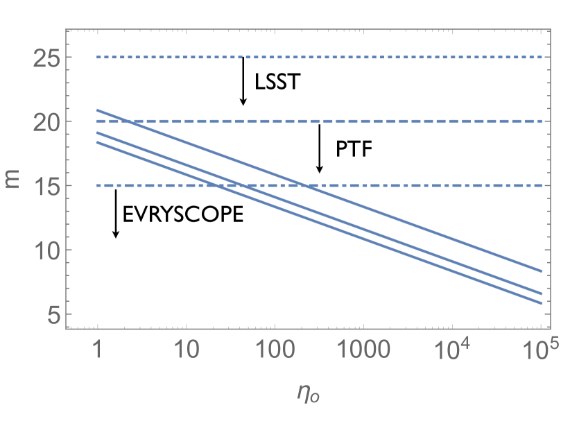
Figure 1: Equivalent stellar magnitude of possible prompt optical emission from an FRB for a 60 s total exposure, as a function of $\eta_{o}$ - ratio of optical to radio energy fluxes for different FRB durations $\tau=1,\,5\,10$ msec (or, equivalently, for different total fluences). As examples of current and future optical transient survey facilities, the expected sensitivities for PTF, LSST and EVRYSCOPE are plotted as the dashed horizontal lines.

Equation (3) also highlights an important fact that shorter readout times are beneficial for the search of optical counterparts to FRBs. Other current facilities that can be used to probe the parameter space shown in Fig. 1 are PAN-STARRS ($m\sim 24$; Tonry et al., 2012), ATLAS ($m\sim 22$; Shanks et al., 2015), ASAS-SN ($m\sim 17$; Holoien et al., 2016) and CRTS ($m\sim$ 19–20; Drake et al., 2009).

The forthcoming Large Synoptic Survey Telescope (LSST; Ivezic et al., 2008) is expected to fare even better. It will also have large field of view, almost 10 square degrees, and will be able to reach magnitude $m=25$ within two exposures of $\sim 15$ s each. So a 6 ms flash has flux about 5000 times smaller than a 30 s exposure. This would produce an image 9.3 magnitudes smaller. Thus, LSST is sensitive to a flash of peak brightness $m=15.2$, about 5 orders of magnitude lower than PTF. In addition, a change in observing strategy - shorter readout times, down to one second - might be used to increase effective sensitivity to transients.

Much larger instantaneous fields of view are about to be explored to shallower magnitude limits by ASAS-SN (Holoien et al., 2016) and EVRYSCOPE (Law et al., 2015). EVRYSCOPE currently samples 8000 deg² fields of view every two minutes. With a magnitude limit of $m=16$, this instrument will be less constraining in terms of $\eta_{o}$ (Fig. 1) compared to PTF and LSST. However, as discussed below, it could provide excellent constraints on optical emission from Lorimer-burst clones.

In conclusion, wide-field deep optical surveys with short exposure time might be able to detect prompt optical emission from FRBs at a level of $m=20$ magnitude. The likelihood of a detection would be even higher if the putative optical luminosity exceeds the radio luminosity by several orders of magnitude. Alternatively, null results from PTF and LSST in future will provide important constraints on prompt optical emission.

2.3 Rates for contemporaneous detections

The all-sky FRB rate of $4.4^{+5.2}_{-3.1}\times 10^{3}$ per day (Rane et al., 2016) implies approximately 0.2–1.6 FRB per 8 square degrees per day (equivalent to PTF or LSST fields of view), or 8–80 FRB per 8000 square degrees per hour (equivalent to EVERYSCOPE). PTF and LSST should, therefore, have an FRB in their field of view every $\sim 12$–90 hours. Since LSST has a very similar field of view this estimate also applies. The average rate of FRB detections at Parkes, based on the survey of Champion et al. (2015) which detected nine FRBs in 2500 hr of observing, is approximately 280 hours per FRB.

The estimate in Equation (3) for the brightness of an optical counterpart can be scaled to other survey telescopes. For example, the BlackGEM telescope (Bloemen et al., 2015) will consist of fifteen telescopes covering total area of 40 square degrees down to $m\sim 20$ in one minute exposure. With the sensitivity similar to PTF, but four times larger area the expected detection rate will be one per few hours. Importantly, using continuous read-out BlackGEM can go to much shorter exposure times, down to few seconds – a transient flash will look brighter for shorter exposure times.

These estimates show that contemporaneous radio-optical detection will be determined mostly by the (relatively small) field of view of radio telescopes. While LOFAR (van Haarlem et al., 2013), with its wide-field coverage might prove effective, e.g., in post-processing analysis of the optically identified flashes, free-free absorption at low frequencies might be important (Lyutikov et al., 2016; Rajwade & Lorimer, 2016). The best prospects for contemporaneous monitoring will most likely come from CHIME (Bandura et al., 2014) or UTMOST (Caleb et al., 2016), where the predicted rates could be up to hundreds of FRBs per day (Rajwade & Lorimer, 2016).

For EVRYSCOPE, the high event rate but shallow sensitivity most likely makes it suitable to bursts from the brightest FRBs. Taking the all-sky event rate for such bursts estimated to be around 250 per day (Lorimer et al., 2007), we find that of order 2 similar bursts would be seen in the EVRYSCOPE field each hour. Inserting $F_{\rm Jy}=30$ and $\tau=15$ ms into Eq. 1, we find $m=15$ for a 2 min exposure if $\eta_{o}=1$. This would be eminently detectable by EVERYSCOPE for which the limiting magnitude is 16.4 in 2 min (Law et al., 2015).

2.4 Radio and high energy GRB-like afterglows

The 2004 flare from SGR 1806–20 produced a total of $4\times 10^{43}$ ergs radio afterglow with peak flux 50 mJy (Gaensler et al., 2005) from a distance of few kpc. Given that the total energetics of the SGR 1806–20 flare was $10^{46}$ ergs (Palmer et al., 2005), the likely radio afterglow efficiency is $4\times 10^{-3}$. Since FRBs are at $d>$ few Mpc, the expected peak flux from a similar radio afterglow would be $<50$ nJy and therefore would not be detectable by current telescopes. At higher energies, no afterglows were observed for SGR 1806–20 (Gaensler et al., 2005). Since FRBs are $\sim 10^{3}$ times further away, we do not expect to see appreciable high-energy afterglows.

On the other hand, there is a possible caveat in the above argument against detectability of afterglow emission. Lyutikov (2006) suggested that though the initial giant flare spike is quasi-isotropic, the ejected relativistically moving magnetic blob (an analog of Solar coronal mass ejections, CMEs) has been collimated into an opening angle $\sim 0.1$ radians. In the case of SGR 1806–20, the motion of the blob was directed away from the observer, so that its emission was de-boosted. If the relativistic CME is directed along the line of sight, we can indeed expect an afterglow which emission is boosted towards an observer lasting $\tau_{\rm ag}\sim$ few weeks. The observed isotropic equivalent luminosity of such afterglow can reach isotropic equivalent luminosity $L_{\rm ag}\sim E_{\rm ej}/(\tau_{\rm ag}\Delta\Omega)\sim 10^{42}$ erg s^-1, where $E_{\rm ej}\sim 10^{46}$ erg is the total energy contained by the CME, $\tau_{\rm ag}\sim 10$ days is the duration of the afterglow and $\Delta\Omega\sim 10^{-2}$ sr is the solid angle of the boosted emission by the relativistically moving CME. For a source located at $\sim 100$ Mpc the corresponding flux at the Earth is relatively high, $\sim 10^{-14}$ erg cm^-2 s^-1. Such transient sources could be detected by existing instruments (e.g.,  XMM sensitivity reaches $\sim 10^{-16}$ erg cm^-2 s^-1). The key drawback of this possibility is that only a small number of magnetar giant flares, $\sim\Delta\Omega\sim 10^{-2}$ sr, is expected to produce CMEs moving along the line of sight.

We note in this respect that the radio afterglow for FRB 150413 claimed by Keane et al. (2016), which was recently argued to be due to AGN variability (Williams & Berger, 2016; Vedantham et al., 2016), generally agrees with these estimates. For example, the afterglow reported by Keane et al. (2016) needs about $10^{45}$ ergs emitted in radio. This is different by about two orders of magnitude from the 2004 flare from SGR 1806$-$20. This increased afterglow luminosity can be due to the mildly relativistic ejection of the CME toward the observer.

3 Summary

In summary, we have discussed several possible strategies for observing possible electromagnetic counterparts of FRBs. If FRBs are related to rotationally-powered giant pulses from newly born “super”-Crab pulsars, we do not expect any other electromagnetic signal. If FRBs are related to magnetar giant flares we can expect (i) to detect the prompt high energy flare; (ii) contemporaneous optical flash that in a $\sim$ 60 seconds exposure can reach equivalent magnitudes of $m\sim 15-20$. In fact, the rate of optical flashes to be seen by PTF and LSST are expected to be higher than the rate of FRBs detected by high frequency searcher. Finally, afterglows can be detected in rare circumstances than the magnetic blob ejected during magnetospheric reconfiguration is moving relativistically towards the observer.

We would like to thank Edo Berger, Paul Groot, Sergey Popov and Matt Wiesner for discussions. This work was supported by NASA grant NNX12AF92G and NSF grants AST-1306672 and AST-1516958.

References

- Aliu et al. (2012) Aliu, E., Archambault, S., Arlen, T., et al. 2012, ApJ, 760, 136
- Bandura et al. (2014) Bandura, K., Addison, G. E., Amiri, M., et al. 2014, in Proc. SPIE, Vol. 9145, Ground-based and Airborne Telescopes V, 914522
- Bilous et al. (2011) Bilous, A. V., Kondratiev, V. I., McLaughlin, M. A., et al. 2011, ApJ, 728, 110
- Bloemen et al. (2015) Bloemen, S., Groot, P., Nelemans, G., & Klein-Wolt, M. 2015, in Astronomical Society of the Pacific Conference Series, Vol. 496, Living Together: Planets, Host Stars and Binaries, ed. S. M. Rucinski, G. Torres, & M. Zejda, 254
- Caleb et al. (2016) Caleb, M., Flynn, C., Bailes, M., et al. 2016, MNRAS, 458, 718
- Camilo et al. (2006) Camilo, F., Ransom, S. M., Halpern, J. P., et al. 2006, Nature, 442, 892
- Champion et al. (2015) Champion, D. J., Petroff, E., Kramer, M., et al. 2015, ArXiv e-prints
- Champion et al. (2016) —. 2016, MNRAS
- Connor et al. (2016) Connor, L., Sievers, J., & Pen, U.-L. 2016, MNRAS, 458, L19
- Cordes & Wasserman (2016) Cordes, J. M., & Wasserman, I. 2016, MNRAS, 457, 232
- Drake et al. (2009) Drake, A. J., Djorgovski, S. G., Mahabal, A., et al. 2009, ApJ, 696, 870
- Eichler et al. (2002) Eichler, D., Gedalin, M., & Lyubarsky, Y. 2002, ApJ, 578, L121
- Gaensler et al. (2005) Gaensler, B. M., Kouveliotou, C., Gelfand, J. D., et al. 2005, Nature, 434, 1104
- Holoien et al. (2016) Holoien, T. W.-S., Stanek, K. Z., Kochanek, C. S., et al. 2016, ArXiv e-prints
- Ivezic et al. (2008) Ivezic, Z., Tyson, J. A., Abel, B., et al. 2008, ArXiv e-prints
- Katz (2015) Katz, J. I. 2015, ArXiv e-prints
- Katz (2016) —. 2016, ArXiv e-prints
- Keane et al. (2012) Keane, E. F., Stappers, B. W., Kramer, M., & Lyne, A. G. 2012, MNRAS, 425, L71
- Keane et al. (2016) Keane, E. F., Johnston, S., Bhandari, S., et al. 2016, Nature, 530, 453
- Law et al. (2009) Law, N. M., Kulkarni, S. R., Dekany, R. G., et al. 2009, PASP, 121, 1395
- Law et al. (2015) Law, N. M., Fors, O., Ratzloff, J., et al. 2015, PASP, 127, 234
- Lorimer et al. (2007) Lorimer, D. R., Bailes, M., McLaughlin, M. A., Narkevic, D. J., & Crawford, F. 2007, Science, 318, 777
- Lundgren et al. (1995) Lundgren, S. C., Cordes, J. M., Ulmer, M., et al. 1995, ApJ, 453, 433
- Lyubarsky (2014) Lyubarsky, Y. 2014, MNRAS, 442, L9
- Lyutikov (2002) Lyutikov, M. 2002, ApJ, 580, L65
- Lyutikov (2006) —. 2006, MNRAS, 367, 1594
- Lyutikov (2007) —. 2007, MNRAS, 381, 1190
- Lyutikov et al. (2016) Lyutikov, M., Burzawa, L., & Popov, S. B. 2016, ArXiv e-prints
- Lyutikov et al. (2012) Lyutikov, M., Otte, N., & McCann, A. 2012, ApJ, 754, 33
- Masui et al. (2015) Masui, K., Lin, H.-H., Sievers, J., et al. 2015, Nature, 528, 523
- Mickaliger et al. (2012) Mickaliger, M. B., McLaughlin, M. A., Lorimer, D. R., et al. 2012, ApJ, 760, 64
- Palmer et al. (2005) Palmer, D. M., Barthelmy, S., Gehrels, N., et al. 2005, Nature, 434, 1107
- Pen & Connor (2015) Pen, U.-L., & Connor, L. 2015, ApJ, 807, 179
- Popov & Postnov (2010) Popov, S. B., & Postnov, K. A. 2010, in Evolution of Cosmic Objects through their Physical Activity, ed. H. A. Harutyunian, A. M. Mickaelian, & Y. Terzian, 129–132
- Rajwade & Lorimer (2016) Rajwade, K. M., & Lorimer, D. R. 2016, MNRAS, submitted
- Rane et al. (2016) Rane, A., Lorimer, D. R., Bates, S. D., et al. 2016, MNRAS, 455, 2207
- Shanks et al. (2015) Shanks, T., Metcalfe, N., Chehade, B., et al. 2015, MNRAS, 451, 4238
- Spitler et al. (2014) Spitler, L. G., Cordes, J. M., Hessels, J. W. T., et al. 2014, ApJ, 790, 101
- Tendulkar et al. (2016) Tendulkar, S. P., Kaspi, V. M., & Patel, C. 2016, ArXiv e-prints
- Thompson et al. (2002) Thompson, C., Lyutikov, M., & Kulkarni, S. R. 2002, ApJ, 574, 332
- Thornton et al. (2013) Thornton, D., Stappers, B., Bailes, M., et al. 2013, Science, 341, 53
- Tonry et al. (2012) Tonry, J. L., Stubbs, C. W., Lykke, K. R., et al. 2012, ApJ, 750, 99
- van Haarlem et al. (2013) van Haarlem, M. P., Wise, M. W., Gunst, A. W., et al. 2013, A&A, 556, A2
- Vedantham et al. (2016) Vedantham, H. K., Ravi, V., Mooley, K., et al. 2016, ArXiv e-prints
- Williams & Berger (2016) Williams, P. K. G., & Berger, E. 2016, ApJ, 821, L22