On the Macroscopic Fractal Geometry
of Some Random Sets

Abstract

This paper is concerned mainly with the macroscopic fractal behavior of various random sets that arise in modern and classical probability theory. Among other things, it is shown here that the macroscopic behavior of Boolean coverage processes is analogous to the microscopic structure of the Mandelbrot fractal percolation. Other, more technically challenging, results of this paper include:

• The computation of the macroscopic dimension of the graph of a large family of Lévy processes; and

• The determination of the macroscopic monofractality of the extreme values of symmetric stable processes.

As a consequence of (i), it will be shown that the macroscopic fractal dimension of the graph of Brownian motion differs from its microscopic fractal dimension. Thus, there can be no scaling argument that allows one to deduce the macroscopic geometry from the microscopic. Item (ii) extends the recent work of Khoshnevisan, Kim, and Xiao [10] on the extreme values of Brownian motion, using a different method.

Keywords: Macroscopic Minkowski dimension, Lévy processes, Boolean models.

AMS 2010 subject classification: Primary 60G51; Secondary. 28A80, 60G17, 60G52.

1 Introduction

It has been known for some time that the curve of a Lévy process in $\mathbb{R}^{d}$ is typically an interesting “random fractal.” For example, if $B=\{B_{t}\}_{t\geqslant 0}$ is a standard Brownian motion on $\mathbb{R}^{d}$, then the image and graph of $B$ have Hausdorff dimension $d\wedge 2$ and $\max(d\wedge 2\,,\nicefrac{{3}}{{2}})$ respectively. If in addition $d=1$, then the level sets of $B$ also have non-trivial Hausdorff dimension $\nicefrac{{1}}{{2}}$. See the survey papers of Taylor [19] and Xiao [20] for historic accounts on these results and further developments.

The beginning student is often presented with some of these “random-fractal facts” via simulation. The well-versed reader will see in Figure 1 a typical example. As a consequence of such a simulation, one is led to believe that one can deduce from a simulation, such as that in Figure 1, the fractal nature of the graph $\cup_{0\leqslant t\leqslant 1}\{(t\,,B_{t})\}$ of Brownian motion up to time $1$.

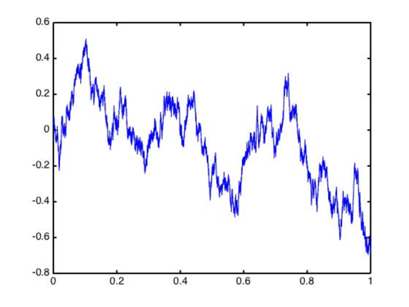
Figure 1: The graph of planar Brownian motion

Figure 1, and other such simulations, are produced by running a random walk for a long time and then rescaling, using a central-limit scaling. The process is usually explained by appealing to Donsker’s invariance principle. Unfortunately, the actual statement of Donsker’s invariance principle is not sufficiently strong to ensure that we can “see” the various fractal properties of Brownian motion in simulations. Though Barlow and Taylor [1, 2] have introduced a theory of large-scale random fractals which, among other things, provides a more rigorous justification.

One of the goals of this paper is to test the extent to which one can experimentally deduce large-scale geometric facts about Brownian motion—and sometimes more general Lévy processes—from simulation analysis. This is achieved by presenting several examples in which one is able to compute the macroscopic fractal dimension of a macroscopic random fractal. One of the surprising lessons of this exercise is that our intuition is, at times, faulty. Yet, our instincts are correct at other times.

Here is an example in which our intuition is spot on: It is known that the level sets of Brownian motion have dimension $\nicefrac{{1}}{{2}}$, both macroscopically and microscopically. This statement has the pleasant consequence that we can “see” the fractal structure of the level sets of Brownian motion from Figure 1. As we shall soon see, however, the same cannot be said of the graph of Brownian motion: The microscopic and macroscopic fractal dimensions of the graph of Brownian motion do not agree!

In order to keep the technical level of the paper as low as possible, our choice of “fractal dimension” is the macroscopic Minkowski dimension, which we will present in the following section. There are more sophisticated notions which, we however, will not present here; see Barlow and Taylor [1, 2] for examples of these more sophisticated notions of macroscopic fractal dimension.

Throughout, ${\rm Log\,}$ denotes the base-2 logarithm. For all $x\in\mathbb{R}^{d}$, we set $|x|:=\max_{1\leqslant j\leqslant d}|x_{j}|$ and $\|x\|:=(x_{1}^{2}+\cdots+x_{d}^{2})^{1/2}$. Whenever we write “$f(x)\lesssim g(x)$ for all $x\in X$,” and/or “$g(x)\gtrsim f(x)$ for all $x\in X$,” we mean that there exists a finite constant $c$ such that $f(x)\leqslant cg(x)$ uniformly for all $x\in X$. If $f(x)\lesssim g(x)$ and $g(x)\lesssim f(x)$ for all $x\in X$, then we write “$f(x)\asymp g(x)$ for all $x\in X$.”

2 Minkowski Dimension

The macroscopic Minkowski dimension is an easy-to-compute “fractal dimension number” that describes the large-scale fractal geometry of a set. In order to recall the Minkowski dimension we first need to introduce some notation.

For all $x\in\mathbb{R}^{d}$ and $r>0$ define

$$B(x;r):=[x_{1}-r\,,x_{1}+r)\times\cdots\times[x_{d}-r\,,x_{d}+r),$$

and

$$Q(x):=[x_{1}\,,x_{1}+1)\times\cdots\times[x_{d}\,,x_{d}+1).$$ (1)

Of course, $Q(x)=B(y;\frac{1}{2})$ where $y_{i}:=x_{i}+\frac{1}{2}$. But it is convenient for $Q(x)$ to have its own notation.

One can introduce a pixelization map which maps a set $F\subseteq\mathbb{R}^{d}$ to a set $\operatorname{\rm pix}(F)\subseteq\mathbb{Z}^{d}$ as follows:

$$\operatorname{\rm pix}(F):=\left\{x\in\mathbb{Z}^{d}:\,F\cap Q(x)\neq\varnothing\right\},$$

for all $F\subseteq\mathbb{R}^{d}$. It is clear that $F=\operatorname{\rm pix}(F)$ if and only if $F$ is a subset of the integer lattice $\mathbb{Z}^{d}$. For example, it should be clear that $\operatorname{\rm pix}(\mathbb{R}^{d})=\mathbb{Z}^{d}$. Figure 2 below shows how the pixelization map works in a different simple case.

Figure 2: The effect of the pixelization map on the ellipse on the left is shown on the right-hand side

The following describes the role of the pixelization map in this paper.

Definition 2.1.

The macroscopic Minkowski dimension of a set $F\subseteq\mathbb{R}^{d}$ is

$$\text{\rm Dim}_{{}_{\rm M}}(F):=\limsup_{n\to\infty}n^{-1}{\rm Log\,}_{+}\left(\left|\operatorname{\rm pix}(F)\cap B(0;2^{n})\right|\right),$$

where $|\,\cdots|$ denotes cardinality and ${\rm Log\,}_{+}(y):=\log_{2}(\max(y\,,2))$.

Remark 2.2.

The right-hand side of (2.1) coincides with the Barlow–Taylor [2] upper mass dimension of the discrete set $\operatorname{\rm pix}(F)\subseteq\mathbb{Z}^{d}$.

The proof of the following elementary result is left to the interested reader.

Lemma 2.3.

For every $A\subseteq\mathbb{R}^{d}$,

$$\text{\rm Dim}_{{}_{\rm M}}(A)=\limsup_{n\to\infty}n^{-1}\log\left|\left\{x\in B(0;2^{n})\cap\mathbb{Z}^{d}:\ Q(x)\cap A\neq\varnothing\right\}\right|,$$

where $Q(x)$ was defined in (1).

Some of the elementary properties of $\text{\rm Dim}_{{}_{\rm M}}$ are listed below:

• If $A\subseteq B$ then $\text{\rm Dim}_{{}_{\rm M}}(A)\leqslant\text{\rm Dim}_{{}_{\rm M}}(B)$;

• If $A$ is a bounded set, then $\text{\rm Dim}_{{}_{\rm M}}(A)=0$;

• $\text{\rm Dim}_{{}_{\rm M}}(\mathbb{R}^{d})=\text{\rm Dim}_{{}_{\rm M}}(\mathbb{Z}^{d})=d$.

The proof is omitted as it is easy to justify the preceding.

2.1 Enumeration in shells

There is a slightly different method of computing the macroscopic Minkowski dimension of a set. With this aim in mind, define

$$\mathcal{S}_{0}:=B(0;1),\qquad\mathcal{S}_{n+1}:=B(0;2^{n+1})\setminus B(0;2^{n})\quad\text{for every integer $n\geqslant 0$.}$$

One can think of $\mathcal{S}_{n}$ as the $n$th shell in $\mathbb{Z}^{d}$.

The following provides an alternative description of $\text{\rm Dim}_{{}_{\rm M}}(F)$.

Proposition 2.4.

For every $F\subseteq\mathbb{R}^{d}$,

$$\text{\rm Dim}_{{}_{\rm M}}(F):=\limsup_{n\to\infty}n^{-1}{\rm Log\,}_{+}\left(\left|\operatorname{\rm pix}(F)\cap\mathcal{S}_{n}\right|\right).$$

Proposition 2.4 tells us that we can replace $\operatorname{\rm pix}(F)\cap B(0;2^{n})$, in Definition 2.1, by $\operatorname{\rm pix}(F)\cap\mathcal{S}_{n}$ without altering the formula for $\text{\rm Dim}_{{}_{\rm M}}(F)$.

Proof.

Our goal is to prove that $\text{\rm Dim}_{{}_{\rm M}}(F)=\delta(F)$, where

$$\delta(F):=\limsup_{n\to\infty}n^{-1}{\rm Log\,}_{+}\left(\left|\operatorname{\rm pix}(F)\cap\mathcal{S}_{n}\right|\right).$$

Since $\mathcal{S}_{n}\subseteq B(0;2^{n})$, the bound $\delta(F)\leqslant\text{\rm Dim}_{{}_{\rm M}}(F)$ is immediate. We will establish the reverse inequality.

The definition of $\delta(F)$ ensures that for every $\varepsilon\in(0\,,1)$ there exists an integer $N(\varepsilon)$ such that

$$\left|\operatorname{\rm pix}(F)\cap\mathcal{S}_{k}\right|\leqslant 2^{k\delta(F)(1+\varepsilon)}\qquad\text{for all $k\geqslant N(\varepsilon)$}.$$

In particular, all $n\geqslant N(\varepsilon)$,

$$\left|\operatorname{\rm pix}(F)\cap B(0;2^{n})\right| =\sum_{k=0}^{n}\left|\operatorname{\rm pix}(F)\cap\mathcal{S}_{k}\right|\leqslant K(\varepsilon)+\sum_{k=N(\varepsilon)}^{n}2^{k\delta(F)(1+\varepsilon)},$$

$$=O\left(2^{n\delta(F)(1+\varepsilon)}\right)\qquad[n\to\infty],$$

where $K(\varepsilon):=\sum_{0\leqslant k<N(\varepsilon)}|\mathcal{S}_{k}|$ is finite and depends only on $(d\,,\varepsilon)$. It follows from Definition 2.1 that $\text{\rm Dim}_{{}_{\rm M}}(F)\leqslant\delta(F)(1+\varepsilon)$. This completes the proof since $\varepsilon\in(0\,,1)$ can be made to be as small as one would like. ∎

2.2 Boolean models

In addition to the method of Proposition 2.4, there is at least one other useful method for computing the macroscopic Minkowski dimension of a set. In contrast with the enumerative method of §2.1, the method of this subsection is intrinsically probabilistic.

Let $\mathbf{p}:=\{p(x)\}_{x\in\mathbb{Z}^{d}}$ denote a collection of numbers in $(0\,,1)$, and refer to the collection $\mathbf{p}$ as coverage probabilities, in keeping with the literature on Boolean coverage processes [6].

Let $\zeta:=\{\zeta(x)\}_{x\in\mathbb{Z}^{d}}$ denote a field of totally independent random variables that satisfy the following for all $x\in\mathbb{Z}^{d}$:

$$\mathrm{P}\{\zeta(x)=1\}=p(x)\quad\text{and}\quad\mathrm{P}\{\zeta(x)=0\}=1-p(x).$$

By a Boolean model in $\mathbb{R}^{d}$ with coverage probabilities $\mathbf{p}$ we mean the random set

$$\mathbf{B}(\mathbf{p}):=\bigcup_{\begin{subarray}{c}x\in\mathbb{Z}^{d}:\\ \zeta(x)=1\end{subarray}}Q(x),$$

where $Q(x)$ was defined earlier in (1).

If $A$ and $B$ are two subsets of $\mathbb{R}^{d}$, then we say that $A$ is recurrent for $B$ if $|A\cap B|=\infty$. Equivalently, $A$ is recurrent for $B$ if $A\cap B\cap\mathcal{S}_{n}\neq\varnothing$ for infinitely-many integers $n\geqslant 0$. Clearly, if $A$ is recurrent for $B$, then $B$ is also recurrent for $A$. Therefore, set recurrence is a symmetric relation.

As the following result shows, it is not hard to decide whether or not a nonrandom Borel set $A\subseteq\mathbb{R}^{d}$ is recurrent for $\mathbf{B}(\mathbf{p})$.

Lemma 2.5.

Let $A\subset\mathbb{R}^{d}$ be a nonrandom Borel set. Then,

$$\mathrm{P}\left\{|A\cap\mathbf{B}(\mathbf{p})|=\infty\right\}=\begin{cases}1&\text{if $\sum_{x\in\operatorname{\rm pix}(A)}p(x)=\infty$},\\ 0&\text{if $\sum_{x\in\operatorname{\rm pix}(A)}p(x)<\infty$}.\end{cases}$$

Lemma 2.5 is basically a reformulation of the Borel–Cantelli lemma for independent events. Therefore, we skip the proof. Instead, let us mention the following, more geometric, result which almost characterizes recurrent sets in terms of their macroscopic Minkowski dimension, in some cases.

Proposition 2.6.

Suppose $\mathbf{p}$ has an index,

$$\text{\rm Ind}(\mathbf{p}):=-\lim_{|x|\to\infty}\frac{\log p(x)}{\log|x|}.$$ (2)

Then for every nonrandom Borel set $A\subseteq\mathbb{R}^{d}$,

$$\mathrm{P}\left\{|A\cap\mathbf{B}(\mathbf{p})|=\infty\right\}=\begin{cases}1&\text{if $\text{\rm Dim}_{{}_{\rm M}}(A)>\text{\rm Ind}(\mathbf{p})$},\\ 0&\text{if $\text{\rm Dim}_{{}_{\rm M}}(A)<\text{\rm Ind}(\mathbf{p})$}.\end{cases}$$

We can compare this result to a similar result of Hawkes [7] about the hitting probabilities of the Mandelbrot fractal percolation. This comparison suggests that the Booelan models of this paper play an analogous role in the theory of macroscopic fractals as does fractal percolation in the better-studied theory of microscopic fractals.

Open Problem.

Is there a macroscopic analogue of the microscopic capacity theory of Peres [15, 16]?

Proof of Proposition 2.6.

Let us consider the process $N_{0},N_{1},N_{2},\ldots$, defined as

$$N_{n}:=|\mathbf{B}(\mathbf{p})\cap A\cap\mathcal{S}_{n}|=\sum_{x\in\operatorname{\rm pix}(A)\cap\mathcal{S}_{n}}\zeta(x)\qquad[n\geqslant 0].$$

Owing to (2) and the definition of $\text{\rm Dim}_{{}_{\rm M}}$,

$$\limsup_{n\to\infty}n^{-1}{\rm Log\,}\mathrm{E}(N_{n})=\text{\rm Dim}_{{}_{\rm M}}(A)-\text{\rm Ind}(\mathbf{p}).$$ (3)

Suppose first that $\text{\rm Dim}_{{}_{\rm M}}(A)<\text{\rm Ind}(\mathbf{p})$. We may combine (3) and Markov’s inequality in order to see that $\sum_{n=1}^{\infty}\mathrm{P}\{N_{n}>0\}\leqslant\sum_{n=1}^{\infty}\mathrm{E}(N_{n})<\infty.$ The Borel–Cantelli lemma then implies that with probability one $N_{n}=0$ for all but finitely-many integers $n$. That is, $|\mathbf{B}(\mathbf{p})\cap A)|<\infty$ a.s. if $\text{\rm Dim}_{{}_{\rm M}}(A)<\text{\rm Ind}(\mathbf{p})$. This proves half of the proposition.

For the remaining half let us assume that $\text{\rm Dim}_{{}_{\rm M}}(A)>\text{\rm Ind}(\mathbf{p})$, and notice that $\operatorname{Var}(N_{n})=\sum_{x\in\operatorname{\rm pix}(A)\cap\mathcal{S}_{n}}p(x)(1-p(x))\leqslant\mathrm{E}(N_{n}).$ Therefore,

$$\mathrm{P}\left\{N_{n}\leqslant\tfrac{1}{2}\mathrm{E}(N_{n})\right\}\leqslant\mathrm{P}\left\{|N_{n}-\mathrm{E}N_{n}|\geqslant\tfrac{1}{2}\mathrm{E}(N_{n})\right\}\leqslant\frac{4\operatorname{Var}(N_{n})}{|\mathrm{E}(N_{n})|^{2}}\leqslant\frac{4}{\mathrm{E}(N_{n})},$$ (4)

thanks to the Chebyshev’s inequality. Because of (4) there exists an infinite collection $\mathcal{N}$ of positive integers such that

$$n^{-1}{\rm Log\,}\mathrm{E}(N_{n})\to\text{\rm Dim}_{{}_{\rm M}}(A)-\text{\rm Ind}(\mathbf{p})>0\qquad\text{as $n$ approaches infinity in $\mathcal{N}$.}$$

This fact, and (3), together imply that $\sum_{n\in\mathcal{N}}\mathrm{P}\{N_{n}\leqslant\frac{1}{2}\mathrm{E}(N_{n})\}<\infty$, and hence

$$\text{\rm Dim}_{{}_{\rm M}}(\mathbf{B}(\mathbf{p})\cap A)=\limsup_{n\to\infty}n^{-1}{\rm Log\,}N_{n}\geqslant\lim_{\begin{subarray}{c}n\to\infty:\\ n\in\mathcal{N}\end{subarray}}n^{-1}{\rm Log\,}N_{n}\geqslant\text{\rm Dim}_{{}_{\rm M}}(A)-\text{\rm Ind}(\mathbf{p})>0,$$

almost surely. This completes the proof. ∎

Remark 2.7.

A quick glance at the proof shows that the independence of the $\zeta$’s was needed only to show that

$$\operatorname{Var}(N_{n})=O(\mathrm{E}(N_{n}))\qquad\text{as $n\to\infty$.}$$ (5)

Because $\operatorname{Var}(N_{n})=\sum_{x,y\in\operatorname{\rm pix}(A)\cap\mathcal{S}_{n}}\mathrm{P}\{\zeta(x)=\zeta(y)=1\}$, (5) continues to hold if the independence of the $\zeta$’s is relaxed to a condition such as the following: There exists finite and positive constants $c$ and $K$ such that

$$\mathrm{P}[\zeta(x)=1\mid\zeta(y)=1]\leqslant c\mathrm{P}\{\zeta(x)=1\}\quad\text{whenever $\|x\|\wedge\|y\|\geqslant K$}.$$

We highlight the power of Proposition 2.6 by using it to give a quick computation of $\text{\rm Dim}_{{}_{\rm M}}(A\cap\mathbf{B}(\mathbf{p}))$.

Corollary 2.8.

If $A\subseteq\mathbb{R}^{d}$ denotes a nonrandom Borel set, then

$$\text{\rm Dim}_{{}_{\rm M}}\left(A\cap\mathbf{B}(\mathbf{p})\right)=\text{\rm Dim}_{{}_{\rm M}}(A)-\text{\rm Ind}(\mathbf{p})\qquad\text{a.s.}$$

Corollary 2.9.

$\text{\rm Dim}_{{}_{\rm M}}(\mathbf{B}(\mathbf{p}))=d-\text{\rm Ind}(\mathbf{p})\qquad\text{a.s.}$

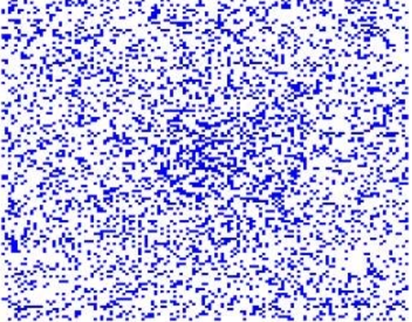
(a) $\text{Ind}({\mathbf{p}})=0.3$, $\text{\rm Dim}_{{}_{\rm M}}(\mathbf{B}(\mathbf{p}))=1.7$

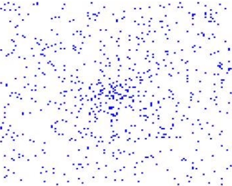
(b) $\text{Ind}({\mathbf{p}})=0.7$, $\text{\rm Dim}_{{}_{\rm M}}(\mathbf{B}(\mathbf{p}))=1.3$

Figure 3: A simulation of two Boolean models. Corollary 2.9 ensures that the Minkowski dimensions of the two figures are respectively $1.7$ (left) and $1.3$ (right).

Because $\text{\rm Dim}_{{}_{\rm M}}(\mathbb{R}^{d})=d$, the following is an immediate consequence of Corollary 2.8. Therefore, it remains to establish Corollary 2.8. The proof uses a variation of an elegant “replica argument” that was introduced by Peres [16] in the context of [microscopic] Hausdorff dimension of fractal percolation processes.

Proof of Corollary 2.8.

Let $\mathbf{B}^{\prime}(\mathbf{p}^{\prime})$ be an independent Boolean model with coverage probabilities $\mathbf{p}^{\prime}=\{p^{\prime}(x)\}_{x\in\mathbb{Z}^{d}}$ that have an index $\text{\rm Ind}(\mathbf{p}^{\prime})$. Define $q(x):=p(x)\times p^{\prime}(x)$ for all $x\in\mathbb{Z}^{d}$. It is then easy to see that $\mathbf{C}(\mathbf{q}):=\mathbf{B}^{\prime}(\mathbf{p}^{\prime})\cap\mathbf{B}(\mathbf{p})$ is a Boolean model with coverage probabilities $\mathbf{q}=\{q(x)\}_{x\in\mathbb{Z}^{d}}$. Since $\text{\rm Ind}(\mathbf{q})=\text{\rm Ind}(\mathbf{p})+\text{\rm Ind}(\mathbf{p}^{\prime})$, Proposition 2.6 implies that

$$\mathrm{P}\left\{|A\cap\mathbf{C}(\mathbf{q})|=\infty\right\}=\begin{cases}1&\text{if $\text{\rm Ind}(\mathbf{p})+\text{\rm Ind}(\mathbf{p}^{\prime})<\text{\rm Dim}_{{}_{\rm M}}(A)$},\\ 0&\text{if $\text{\rm Ind}(\mathbf{p})+\text{\rm Ind}(\mathbf{p}^{\prime})>\text{\rm Dim}_{{}_{\rm M}}(A)$}.\end{cases}$$

At the same time, one can apply Proposition 2.6 conditionally in order to see that almost surely,

$$\mathrm{P}\left(|A\cap\mathbf{C}(\mathbf{q})|=\infty\mid\mathbf{B}(\mathbf{p})\right) =\mathrm{P}\left(|A\cap\mathbf{B}(\mathbf{p})\cap\mathbf{B}^{\prime}(\mathbf{p^{\prime}})|=\infty\mid\mathbf{B}(\mathbf{p})\right)$$

$$=\begin{cases}1&\text{if $\text{\rm Dim}_{{}_{\rm M}}\left(A\cap\mathbf{B}(\mathbf{p})\right)>\text{\rm Ind}(\mathbf{p^{\prime}})$},\\ 0&\text{if $\text{\rm Dim}_{{}_{\rm M}}\left(A\cap\mathbf{B}(\mathbf{p})\right)<\text{\rm Ind}(\mathbf{p^{\prime}})$}.\end{cases}$$

A comparison of the preceding two displays yields the following almost sure assertions:

1. If $\text{\rm Ind}(\mathbf{p})+\text{\rm Ind}(\mathbf{p}^{\prime})<\text{\rm Dim}_{{}_{\rm M}}(A)$, then $\text{\rm Dim}_{{}_{\rm M}}\left(A\cap\mathbf{B}(\mathbf{p})\right)\geqslant\text{\rm Ind}(\mathbf{p^{\prime}})$ a.s.; and

2. If $\text{\rm Ind}(\mathbf{p})+\text{\rm Ind}(\mathbf{p}^{\prime})>\text{\rm Dim}_{{}_{\rm M}}(A)$, then $\text{\rm Dim}_{{}_{\rm M}}\left(A\cap\mathbf{B}(\mathbf{p})\right)\leqslant\text{\rm Ind}(\mathbf{p^{\prime}})$ a.s.

Since $\mathbf{p}^{\prime}$ can have any arbitrary index $\text{\rm Ind}(\mathbf{p}^{\prime})>0$ that one wishes, the corollary follows. ∎

3 Transient Lévy processes

Let $X:=\{X_{t}\}_{t\geqslant 0}$ be a Lévy process on $\mathbb{R}^{d}$. That is, $X$ is a strong Markov process that has càdlàg paths, takes values in $\mathbb{R}^{d}$, $X_{0}=0$, and $X$ has stationary and independent increments. See, for example, Bertoin [3] for a pedagogic account. In this section we assume that $X$ is transient and compute the macroscopic dimension of the range $\mathcal{R}_{{}_{X}}$ of $X$, where we recall the range is the following random set:

$$\mathcal{R}_{{}_{X}}:=\bigcup_{t\geqslant 0}\{X_{t}\}.$$

3.1 The potential measure

Let $\mathrm{U}_{{}_{X}}$ denote the potential measure of $X$; that is,

$$\mathrm{U}_{{}_{X}}(A):=\int_{0}^{\infty}\mathrm{P}\{X_{t}\in A\}\,{\rm d}t=\mathrm{E}\int_{0}^{\infty}\mathds{1}_{A}(X_{t})\,{\rm d}t.$$ (6)

Throughout we assume that $X$ is transient; equivalently, $\mathrm{U}_{{}_{X}}$ is a Radon measure. The following shows that the macroscopic Minkowski dimension of the range of $X$ is linked intimately to the potential measure of $X$.

Theorem 3.1.

With probability one,

$$\text{\rm Dim}_{{}_{\rm M}}(\mathcal{R}_{{}_{X}})=\inf\left\{\alpha>0:\ \int_{\mathbb{R}^{d}}\frac{\mathrm{U}_{{}_{X}}({\rm d}x)}{1+|x|^{\alpha}}<\infty\right\}.$$

Theorem 3.9 contains an alternative formula for $\text{\rm Dim}_{{}_{\rm M}}(\mathcal{R}_{{}_{X}})$, in terms of the Lévy exponent of $X$, which is reminiscent of an old formula of Pruitt [18] for the [micrsoscopic] Hausdorff dimension of $\mathcal{R}_{{}_{X}}$. We refer to Ref.’s [11, 12, 13] for more recent developments on micrsoscopic fractal properties of Lévy processes, based on potential theory of additive Lévy processes.

Example 3.2.

Consider the case that $X:=\{X_{t}\}_{t\geqslant 0}$ is a symmetric $\beta$-stable process on $\mathbb{R}^{d}$ for some $0<\beta\leqslant 2$. Transience is equivalent to the condition $\alpha<d$. This condition is known to imply that $\mathrm{U}_{{}_{X}}({\rm d}x)/{\rm d}x\propto\|x\|^{-d+\beta}$ for all $x\in\mathbb{R}^{d}\setminus\{0\}$ [3, 17]. Therefore, $\int_{\mathbb{R}^{d}}(1+|x|^{\alpha})^{-1}\,\mathrm{U}_{{}_{X}}({\rm d}x)<\infty$ iff $\int_{|x|>1}|x|^{-\alpha-d+\beta}\,{\rm d}x<\infty$ iff $\alpha>\beta$. Theorem 3.1 then implies that $\text{\rm Dim}_{{}_{\rm M}}(\mathcal{R}_{{}_{X}})=\beta$ a.s. This fact is essentially due to Barlow and Taylor [2].

Remark 3.3.

Recall that the measure $\mathrm{U}_{{}_{X}}$ is finite because $X$ is transient. As a result, $\int_{\mathbb{R}^{d}}(1+|x|^{\alpha})^{-1}\,\mathrm{U}_{{}_{X}}({\rm d}x)$ converges iff $\int_{|x|>1}|x|^{-\alpha}\,\mathrm{U}_{{}_{X}}({\rm d}x)<\infty$. One can then deduce from this fact, from the definition (6) of $\mathrm{U}_{{}_{X}}$, and from Theorem 3.1 that

$$\text{\rm Dim}_{{}_{\rm M}}(\mathcal{R}_{{}_{X}})=\inf\left\{\alpha>0:\ \int_{0}^{\infty}\mathrm{E}\left(|X_{t}|^{-\alpha};|X_{t}|>1\right){\rm d}t<\infty\right\}\qquad\text{a.s.}$$

This is the macroscopic analogue of a result of Pruitt [18, p. 374].

Open Problem.

It is natural to ask if there is a nice formula for $\text{\rm Dim}_{{}_{\rm M}}(A\cap\mathcal{R}_{{}_{X}})$ when $A\subseteq\mathbb{R}^{d}$ is Borel and nonrandom. We do not have an answer to this question when $A$ is not “macroscopically self-similar.”

The proof of Theorem 3.1 hinges on a few prefatory technical results. The first is a more-or-less well-known set of bounds on the potential measure of a ball.

Lemma 3.4.

For every $x\in\mathbb{R}^{d}$ and $r>0$,

$$\mathrm{U}_{{}_{X}}(B(x;r))\leqslant\mathrm{U}_{{}_{X}}(B(0;2r))\cdot\mathrm{P}\left\{\overline{\mathcal{R}_{{}_{X}}}\cap B(x;r)\neq\varnothing\right\}.$$

Proof.

Let $\inf\varnothing:=\infty$, and consider the stopping time

$$T(x;r):=\inf\{t\geqslant 0:X_{t}\in B(x;r)\}.$$ (7)

We can write $\mathrm{U}_{{}_{X}}(B(x;r))$ in the following equivalent form:

$$\mathrm{E}\left(\int_{0}^{\infty}\mathds{1}_{B(x-X_{T(x;r)},r)}\left(X_{t+T(x;r)}-X_{T(x;r)}\right){\rm d}t\cdot\mathds{1}_{\{T(x;r)<\infty\}}\right).$$ (8)

Since $|X_{T(x;r)}-x|<r$ a.s. on the event $\{T(x;r)<\infty\}$, the triangle inequality implies that $B(x-X_{T(x;r)}\,,r)\subseteq B(0;2r)$ a.s. on $\{T(x;r)<\infty\}$, and hence

$$\mathrm{U}_{{}_{X}}(B(x;r))\leqslant\mathrm{U}_{{}_{X}}(B(0;2r))\cdot\mathrm{P}\{T(x;r)<\infty\}.$$

This is another way to state the lemma. ∎

The next result is a standard upper bound on the hitting probability of a ball.

Lemma 3.5.

For every $x\in\mathbb{R}^{d}$ and $r>0$,

$$\mathrm{U}_{{}_{X}}(B(x;2r))\geqslant\mathrm{U}_{{}_{X}}(B(0;r))\cdot\mathrm{P}\left\{\overline{\mathcal{R}_{{}_{X}}}\cap B(x;r)\neq\varnothing\right\}.$$

Proof.

By the triangle inequality, $B(x-X_{T(x;r)}\,,2r)\supset B(0;r)$ almost surely on the event $\{T(x;r)<\infty\}$, where $T(x;r)$ was defined in (7). Therefore, we apply (8) together with the strong Markov property in order to see that

$$\mathrm{U}_{{}_{X}}(B(x;2r))\geqslant\mathrm{U}_{{}_{X}}(B(0;r))\cdot\mathrm{P}\{T(x;r)<\infty\}.$$

This is another way to write the lemma. ∎

The following is a “weak unimodality” result for the potential measure.

Lemma 3.6.

$\mathrm{U}_{{}_{X}}(B(x;r))\leqslant 4^{d}\mathrm{U}_{{}_{X}}(B(0;r))$ for all $x\in\mathbb{R}^{d}$ and $r>0$.

Proof.

The proof will use the following elementary covering property of Euclidean spaces: For every $x\in\mathbb{R}^{d}$ and $r>0$ there exist points $y_{1},\ldots,y_{4^{d}}\in B(x;r)$ such that $B(x;r)=\cup_{1\leqslant i\leqslant 4^{d}}B(y_{i}\,,r/2).$ This leads to the following “volume-doubling” bound: For all $r>0$ and $x\in\mathbb{R}^{d}$,

$$\mathrm{U}_{{}_{X}}(B(x;r))\leqslant 4^{d}\sup_{y\in B(x,r)}\mathrm{U}_{{}_{X}}(B(y;r/2)).$$ (9)

This inequality yields the lemma since $\mathrm{U}_{{}_{X}}(B(y;r/2))\leqslant\mathrm{U}_{{}_{X}}(B(0;r))$ for all $y\in\mathbb{R}^{d}$ and $r>0$, thanks to Lemma 3.4. ∎

The next result presents bounds for the probability that the pixelization of the range of $X$ hits singletons. Naturally, both bounds are in terms of the potential measure of $X$.

Lemma 3.7.

There exist finite constants $c_{2}>1>c_{1}>0$ such that, for all $x\in\mathbb{Z}^{d}$,

$$c_{1}\mathrm{U}_{{}_{X}}(Q(x))\leqslant\mathrm{P}\left\{x\in\operatorname{\rm pix}\left(\mathcal{R}_{{}_{X}}\right)\right\}\leqslant c_{2}\mathrm{U}_{{}_{X}}(B(x;2)).$$

Proof.

Since the process $X$ is càdlàg, the difference between $\mathcal{R}_{{}_{X}}$ and its closure is a.s. denumerable, and hence

$$\mathrm{P}\left\{x\in\operatorname{\rm pix}\left(\mathcal{R}_{{}_{X}}\right)\right\}=\mathrm{P}\left\{x\in\operatorname{\rm pix}\left(\overline{\mathcal{R}_{{}_{X}}}\right)\right\}=\mathrm{P}\left\{\overline{\mathcal{R}_{{}_{X}}}\cap Q(x)\neq\varnothing\right\},$$

for all $x\in\mathbb{Z}^{d}$. Let $y_{i}:=x_{i}+\frac{1}{2}$ for $1\leqslant i\leqslant d$ and recall that $Q(x)=B(y;1/2)$ in order to deduce from Lemmas 3.4 and 3.5 that

$$\frac{\mathrm{U}_{{}_{X}}(Q(x))}{\mathrm{U}_{{}_{X}}(B(0;1))}=\frac{\mathrm{U}_{{}_{X}}(B(y;1/2))}{\mathrm{U}_{{}_{X}}(B(0;1))}\leqslant\mathrm{P}\left\{x\in\operatorname{\rm pix}\left(\mathcal{R}_{{}_{X}}\right)\right\}\leqslant\frac{\mathrm{U}_{{}_{X}}(B(y;1))}{\mathrm{U}_{{}_{X}}(B(0;1/2))}.$$ (10)

The denominators are strictly positive because $X$ is càdlàg and $B(0;1/2)$ is open in $\mathbb{R}^{d}$; and they are finite because of the transience of $X$. Because $B(y;1)\subseteq B(x;2)$, (10) completes the proof. ∎

The following lemma is the final technical result of this section. It presents an upper bound for the probability that the range of $X$ simultaneously intersects two given balls.

Lemma 3.8.

For all $x,y\in\mathbb{R}^{d}$ and $r>0$,

$$\mathrm{P}\left\{\overline{\mathcal{R}}_{X}\cap B(x;r)\neq\varnothing\,,\overline{\mathcal{R}_{{}_{X}}}\cap B(y;r)\neq\varnothing\right\}$$

$$\hskip 72.26999pt\leqslant\frac{\mathrm{U}_{{}_{X}}(B(x;2r))}{\mathrm{U}_{{}_{X}}(B(0;r))}\cdot\frac{\mathrm{U}_{{}_{X}}(B(y-x;4r))}{\mathrm{U}_{{}_{X}}(B(0;2r))}+\frac{\mathrm{U}_{{}_{X}}(B(y;2r))}{\mathrm{U}_{{}_{X}}(B(0;r))}\cdot\frac{\mathrm{U}_{{}_{X}}(B(x-y;4r))}{\mathrm{U}_{{}_{X}}(B(0;2r))}.$$

Proof.

Let us recall the stopping times $T(x;r)$ from (7). First one notices that

$$\mathrm{P}\left\{T(x;r)\leqslant T(y;r)<\infty\right\} =\mathrm{P}\left\{T(x;r)<\infty,\,\exists s\geqslant 0:X_{s+T(x;r)}-X_{T(x;r)}\in B(y-X_{T(x;r)};r)\right\}$$

$$\leqslant\mathrm{P}\{T(x;r)<\infty\}\cdot\mathrm{P}\{T(y-x;2r)<\infty\}$$

$$=\mathrm{P}\left\{\overline{\mathcal{R}_{{}_{X}}}\cap B(x;r)\neq\varnothing\right\}\cdot\mathrm{P}\left\{\overline{\mathcal{R}_{{}_{X}}}\cap B(y-x;2r)\neq\varnothing\right\},$$

owing to the strong Markov property and the fact that $B(y-X_{T(x;r)}\,,r)\subseteq B(y-x;2r)$ a.s. on $\{T(x;r)<\infty\}$ [the triangle inequality]. By replacing also the roles of $x$ and $y$ and appealing to the subadditivity of probabilities, one can deduce from the preceding that

$$\mathrm{P}\left\{\overline{\mathcal{R}}_{X}\cap B(x;r)\neq\varnothing\,,\overline{\mathcal{R}_{{}_{X}}}\cap B(y;r)\neq\varnothing\right\}$$

$$\hskip 72.26999pt\leqslant\mathrm{P}\left\{\overline{\mathcal{R}_{{}_{X}}}\cap B(x;r)\neq\varnothing\right\}\cdot\mathrm{P}\left\{\overline{\mathcal{R}_{{}_{X}}}\cap B(y-x;2r)\neq\varnothing\right\}$$

$$\hskip 180.67499pt+\mathrm{P}\left\{\overline{\mathcal{R}_{{}_{X}}}\cap B(y;r)\neq\varnothing\right\}\cdot\mathrm{P}\left\{\overline{\mathcal{R}_{{}_{X}}}\cap B(x-y;2r)\neq\varnothing\right\}.$$

An appeal to Lemma 3.5 completes the proof. ∎

With the requisite material for the proof of Theorem 3.1 under way, we are ready for the following.

Proof of Theorem 3.1.

The strategy of the proof is to verify that $\text{\rm Dim}_{{}_{\rm M}}(\mathcal{R}_{{}_{X}})=\alpha_{c}$ a.s., where

$$\alpha_{c}:=\inf\left\{\alpha>0:\ \int_{\mathbb{R}^{d}}\frac{\mathrm{U}_{{}_{X}}({\rm d}x)}{1+|x|^{\alpha}}<\infty\right\}.$$

Let us begin by making some real-variable observations. First, let us note that because $\mathrm{U}_{{}_{X}}$ is a finite measure [by transience],

$$\sum_{n=1}^{\infty}2^{-n\alpha}\mathrm{U}_{{}_{X}}(\mathcal{S}_{n})=\sum_{n=1}^{\infty}2^{-n\alpha}\int_{\mathcal{S}_{n}}\mathrm{U}_{{}_{X}}({\rm d}x)\asymp\int_{|x|>1}\frac{\mathrm{U}_{{}_{X}}({\rm d}x)}{|x|^{\alpha}}\asymp\int_{\mathbb{R}^{d}}\frac{\mathrm{U}_{{}_{X}}({\rm d}x)}{1+|x|^{\alpha}}.$$

Therefore,

$$\alpha_{c}=\inf\left\{\alpha>0:\ \sum_{n=1}^{\infty}2^{-n\alpha}\mathrm{U}_{{}_{X}}(\mathcal{S}_{n})<\infty\right\}.$$

By the definition of $\alpha_{c}$, if $0<\alpha<\alpha_{c}$, then $\sum_{n}2^{-n\alpha}\mathrm{U}_{{}_{X}}(\mathcal{S}_{n})=\infty$; as a result,

$$\limsup_{n\to\infty}2^{-\beta n}\mathrm{U}_{{}_{X}}(B(0;2^{n}))\geqslant\limsup_{n\to\infty}2^{-\beta n}\mathrm{U}_{{}_{X}}(\mathcal{S}_{n})=\infty,$$

whenever $0<\beta<\alpha$. On the other hand, if $\beta>\alpha_{c}$, then $\limsup_{n\to\infty}2^{-\beta n}\mathrm{U}_{{}_{X}}(\mathcal{S}_{n})<\infty$, and hence

$$\mathrm{U}_{{}_{X}}(B(0;2^{n}))=\sum_{k=0}^{n}\mathrm{U}_{{}_{X}}(\mathcal{S}_{k})=O(2^{\beta n})\qquad\text{as $n\to\infty$.}$$

These remarks together show the following alternative representation of $\alpha_{c}$:

$$\alpha_{c}=\limsup_{n\to\infty}n^{-1}{\rm Log\,}\mathrm{U}_{{}_{X}}(B(0;2^{n}))=\limsup_{n\to\infty}n^{-1}{\rm Log\,}\mathrm{U}_{{}_{X}}(\mathcal{S}_{n}).$$ (11)

Now we begin the bulk of the proof.

Because $X$ has càdlàg sample functions, Lemma 3.7 and (11) together imply that for all $n\geqslant 2$,

$$\mathrm{E}\left|\operatorname{\rm pix}\left(\mathcal{R}_{{}_{X}}\right)\cap B(0;2^{n})\right|\lesssim\sum_{x\in B(0;2^{n})}\mathrm{U}_{{}_{X}}(B(x;2))\lesssim\mathrm{U}_{{}_{X}}(B(0;2^{n+1}))\leqslant 2^{n(1+o(1))\text{\rm Dim}_{{}_{\rm M}}(\mathcal{R}_{{}_{X}})},$$

as $n\to\infty$. Therefore, the Chebyshev inequality implies that

$$\sum_{n=1}^{\infty}\mathrm{P}\left\{\left|\operatorname{\rm pix}\left(\mathcal{R}_{{}_{X}}\right)\cap B(0;2^{n})\right|>2^{n\theta}\right\}<\infty\qquad\text{for all $\theta>\alpha_{c}$}.$$

An application of the Borel–Cantelli lemma yields $\text{\rm Dim}_{{}_{\rm M}}(\mathcal{R}_{{}_{X}})\leqslant\alpha_{c}$ a.s., which implies a part of the assertion of the theorem.

For the next part, let us begin with the following consequence of Lemma 3.7:

$$\mathrm{E}\left|\operatorname{\rm pix}\left(\mathcal{R}_{{}_{X}}\right)\cap B(0;2^{n})\right|\gtrsim\sum_{x\in B(0;2^{n})}\mathrm{U}_{{}_{X}}(Q(x))\asymp\mathrm{U}_{{}_{X}}(B(0;2^{n})).$$ (12)

Next, we estimate the second moment of the same random variable as follows:

$$\mathrm{E}\left(\left|\operatorname{\rm pix}\left(\mathcal{R}_{{}_{X}}\right)\cap B(0;2^{n})\right|^{2}\right) \leqslant\sum_{x,y\in B(0;2^{n})}\mathrm{P}\left\{\overline{\mathcal{R}}_{X}\cap B(x;1)\neq\varnothing\,,\overline{\mathcal{R}_{{}_{X}}}\cap B(y;1)\neq\varnothing\right\}$$

$$\leqslant\sum_{x,y\in B(0;2^{n})}\frac{\mathrm{U}_{{}_{X}}(B(x;2))}{\mathrm{U}_{{}_{X}}(B(0;1))}\cdot\frac{\mathrm{U}_{{}_{X}}(B(y-x;4))}{\mathrm{U}_{{}_{X}}(B(0;2))}$$

$$\hskip 72.26999pt+\sum_{x,y\in B(0;2^{n})}\frac{\mathrm{U}_{{}_{X}}(B(y;2))}{\mathrm{U}_{{}_{X}}(B(0;1))}\cdot\frac{\mathrm{U}_{{}_{X}}(B(x-y;4))}{\mathrm{U}_{{}_{X}}(B(0;2))};$$

see Lemma 3.8 for the final inequality. Since $B(0;2^{n})\ominus B(0;2^{n})=B(0\,,2^{n+1})$, it follows that

$$\mathrm{E}\left(\left|\operatorname{\rm pix}\left(\mathcal{R}_{{}_{X}}\right)\cap B(0;2^{n})\right|^{2}\right) \leqslant 2\sum_{x\in B(0;2^{n})}\frac{\mathrm{U}_{{}_{X}}(B(x;2))}{\mathrm{U}_{{}_{X}}(B(0;1))}\ \cdot\sum_{w\in B(0;2^{n+1})}\frac{\mathrm{U}_{{}_{X}}(B(w;4))}{\mathrm{U}_{{}_{X}}(B(0;2))}$$

$$\leqslant K\mathrm{U}_{{}_{X}}(B(0;2^{n+1}))\cdot\mathrm{U}_{{}_{X}}(B(0;2^{n+2})$$

$$\leqslant 4^{3d}K[\mathrm{U}_{{}_{X}}(B(0;2^{n}))]^{2},$$

where $K:=2[\mathrm{U}_{{}_{X}}(B(0;1))\mathrm{U}_{{}_{X}}(B(0;2))]^{-1}$ and the last line follows from (9). Therefore, the Paley–Zygmund inequality and (12) together imply that

$$\mathrm{P}\left\{\left|\operatorname{\rm pix}\left(\mathcal{R}_{{}_{X}}\right)\cap B(0;2^{n})\right|>\frac{c_{1}}{2}\mathrm{U}_{{}_{X}}(B(0;2^{n}))\right\} \geqslant\frac{\left(\mathrm{E}\left|\operatorname{\rm pix}\left(\mathcal{R}_{{}_{X}}\right)\cap B(0;2^{n})\right|\right)^{2}}{4\mathrm{E}\left(\left|\operatorname{\rm pix}\left(\mathcal{R}_{{}_{X}}\right)\cap B(0;2^{n})\right|^{2}\right)}$$

$$\gtrsim 1,$$

uniformly in $n$. The preceding and (11) together imply that $\text{\rm Dim}_{{}_{\rm M}}(\mathcal{R}_{{}_{X}})\geqslant\alpha_{c}$ a.s. This verifies the theorem since the other bound was verified earlier in the proof. ∎

3.2 Fourier analysis

It is well-known that the law of $X$ is determined by a socalled characteristic exponent $\Psi_{{}_{X}}:\mathbb{R}^{d}\to\mathbb{C}$, which can be defined via $\mathrm{E}\exp(iz\cdot X_{t})=\exp(-t\Psi_{{}_{X}}(z))$ for all $t\geqslant 0$ and $z\in\mathbb{R}^{d}$. In particular, one can prove from this that $\Psi_{{}_{X}}(z)\neq 0$ for almost all $z\in\mathbb{R}^{d}$. This fact is used tacitly in the sequel.

We frequently use the well-known fact that ${\rm Re}\Psi_{{}_{X}}(z)\geqslant 0$ for all $z\in\mathbb{R}^{d}$. To see this fact, let $X^{\prime}$ be an independent copy of $X$ and note that $t\mapsto X_{t}-X_{t}^{\prime}$ is a Lévy process with characteristic exponent $2{\rm Re}\Psi_{{}_{X}}$. Since $X_{1}-X^{\prime}_{1}$ is a symmetric random variable, one can conclude the mentioned fact that ${\rm Re}\Psi_{{}_{X}}\geqslant 0$.

Port and Stone [17] have proved, among other things, that the transience of $X$ is equivalent to the convergence of the integral

$$I(\Psi_{{}_{X}}):=\int_{\|z\|\leqslant 1}{\rm Re}\left(\frac{1}{\Psi_{{}_{X}}(z)}\right){\rm d}z;$$

see also [3]. The following shows that the macroscopic dimension of the range of $X$ is determined by the strength by which the Port–Stone integral $I(\Psi_{{}_{X}})$ converges.

Theorem 3.9.

With probability one,

$$\text{\rm Dim}_{{}_{\rm M}}(\mathcal{R}_{{}_{X}})=\inf\left\{\alpha>0:\ \int_{\|z\|\leqslant 1}{\rm Re}\left(\frac{1}{\Psi_{{}_{X}}(z)}\right)\frac{{\rm d}z}{\|z\|^{d-\alpha}}<\infty\right\}.$$

The proof of Theorem 3.9 hinges on a calculation from classical Fourier analysis. From now on, $\widehat{h}$ denotes the Fourier transform of a locally integrable function $h:\mathbb{R}^{d}\to\mathbb{R}$, normalized so that

$$\widehat{h}(z)=\int_{\mathbb{R}^{d}}{\rm e}^{iz\cdot x}h(x)\,{\rm d}x\qquad\text{for all $z\in\mathbb{R}^{d}$ and $h\in L^{1}(\mathbb{R}^{d}$)}.$$

As is done customarily, we let $K_{\nu}$ denote the modified Bessel function [Macdonald function] of the second kind.

Lemma 3.10.

Choose and fix $\alpha>0$ and define $f(x):=(1+\|x\|^{2})^{-\alpha/2}$ for all $x\in\mathbb{R}^{d}$. Then, the Fourier transform of $f$ is

$$\widehat{f}(z)=c_{d,\alpha}\cdot\frac{K_{(d-\alpha)/2}(\|z\|)}{\|z\|^{(d-\alpha)/2}}\qquad[z\in\mathbb{R}^{d}],$$

where $0<c_{d,\alpha}<\infty$ depends only on $(d\,,\alpha)$.

Proof.

This is undoubtedly well known; the proof hinges on a simple abelian trick that can be included with little added effort.

For all $x\in\mathbb{R}^{d}$ and $\theta>0$,

$$\int_{0}^{\infty}{\rm e}^{-t(1+\|x\|^{2})}t^{\theta-1}\,{\rm d}t=\frac{\Gamma(\theta)}{(1+\|x\|^{2})^{\theta}}.$$

Therefore, for every rapidly decreasing test function $\varphi:\mathbb{R}^{d}\to\mathbb{R}$,

$$\int_{\mathbb{R}^{d}}\frac{\varphi(x)}{(1+\|x\|^{2})^{\theta}}\,{\rm d}x =\frac{1}{\Gamma(\theta)}\int_{\mathbb{R}^{d}}\varphi(x)\,{\rm d}x\int_{0}^{\infty}{\rm d}t\ {\rm e}^{-t(1+\|x\|^{2})}t^{\theta-1}$$

$$=\frac{1}{\Gamma(\theta)}\int_{0}^{\infty}{\rm e}^{-t}t^{\theta-1}\,{\rm d}t\int_{\mathbb{R}^{d}}\varphi(x){\rm e}^{-t\|x\|^{2}}\,{\rm d}x.$$

Since

$$\int_{\mathbb{R}^{d}}\varphi(x){\rm e}^{-t\|x\|^{2}}\,{\rm d}x=(4\pi t)^{-d/2}\int_{\mathbb{R}^{d}}\overline{\widehat{\varphi}(z)}\exp\left(-\frac{\|z\|^{2}}{4t}\right){\rm d}z,$$

it follows that

$$\int_{\mathbb{R}^{d}}\frac{\varphi(x)}{(1+\|x\|^{2})^{\theta}}\,{\rm d}x =\frac{1}{b}\int_{\mathbb{R}^{d}}\overline{\widehat{\varphi}(z)}\,{\rm d}z\int_{0}^{\infty}\frac{{\rm d}t}{t^{(d/2)-\theta+1}}\exp\left(-t-\frac{\|z\|^{2}}{4t}\right){\rm d}z$$

$$=\frac{1}{c}\int_{\mathbb{R}^{d}}\overline{\widehat{\varphi}(z)}\,\frac{K_{(d/2)-\theta}(\|z\|)}{\|z\|^{(d/2)-\theta}}\,{\rm d}z,$$

where $b:=(4\pi)^{d/2}\Gamma(\theta)$ and $c:=(4\pi)^{d/2}\Gamma(\theta)2^{-1-(d/2)+\theta}$. This proves the result, after we set $\theta:=\alpha/2$. ∎

Proof of Theorem 3.9.

It is not hard to check (see, for example, Port and Stone [17]) that $\widehat{\mathrm{U}}_{{}_{X}}(z)=1/\Psi_{{}_{X}}(z)$ for almost all $z\in\mathbb{R}^{d}$. Because ${\rm Re}(1/\Psi_{{}_{X}}(z))={\rm Re}\Psi_{{}_{X}}(z)/|\Psi_{{}_{X}}(z)|^{2}>0$ a.e., Lemma 3.10 and a suitable form of the Plancherel’s theorem together imply that

$$\int_{\mathbb{R}^{d}}\frac{\mathrm{U}_{{}_{X}}({\rm d}x)}{1+|x|^{\alpha}}\asymp\int_{\mathbb{R}^{d}}\frac{\mathrm{U}_{{}_{X}}({\rm d}x)}{(1+|x|^{2})^{\alpha/2}}\propto\int_{\mathbb{R}^{d}}{\rm Re}\left(\frac{1}{\Psi_{{}_{X}}(z)}\right)\frac{K_{(d-\alpha)/2}(\|z\|)}{\|z\|^{(d-\alpha)/2}}\,{\rm d}z:=T_{1}+T_{2},$$

where $T_{1}$ denotes the preceding integral with domain of integration restricted to $\{z\in\mathbb{R}^{d}:\,|\Psi(z)|<1\}$ and $T_{2}$ is the same integral over $\{z\in\mathbb{R}^{d}:\,|\Psi(z)|\geqslant 1\}$.

A standard application of Laplace’s method shows that for all $R>0$ there exists a finite $A>1$ such that

$$\frac{{\rm e}^{-w}}{A\sqrt{w}}\leqslant K_{\nu}(w)\leqslant\frac{A{\rm e}^{-w}}{\sqrt{w}},$$

whenever $w>R$. And one can check directly that for all $R>0$ we can find a finite $B>1$ such that

$$B^{-1}w^{-\nu}\leqslant K_{\nu}(w)\leqslant Bw^{-\nu}\qquad\text{whenever $0<w<R$.}$$

Since $\Psi_{{}_{X}}:\mathbb{R}^{d}\to\mathbb{C}$ is a continuous function that vanishes at the origin, $\{z\in\mathbb{R}^{d}:\,|\Psi_{{}_{X}}(z)|>1\}$ does not intersect a certain ball about the origin of $\mathbb{R}^{d}$. Therefore, the inequality ${\rm Re}(1/\Psi_{{}_{X}}(z))\leqslant|\Psi_{{}_{X}}(z)|^{-1}$, valid for all $z\in\mathbb{R}^{d}$, implies that

$$T_{1} \asymp\int_{|\Psi_{{}_{X}}(z)|\leqslant 1}{\rm Re}\left(\frac{1}{\Psi_{{}_{X}}(z)}\right)\frac{{\rm d}z}{\|z\|^{d-\alpha}},$$

and

$$T_{2} \asymp\int_{|\Psi_{{}_{X}}(z)|\geqslant 1}{\rm Re}\left(\frac{1}{\Psi_{{}_{X}}(z)}\right)\frac{{\rm e}^{-\|z\|}}{\|z\|^{(d-\alpha+1)/2}}\,{\rm d}z\leqslant\int_{|\Psi_{{}_{X}}(z)|\geqslant 1}\frac{{\rm e}^{-\|z\|}}{\|z\|^{(d-\alpha+1)/2}}\,{\rm d}z<\infty.$$

This verifies that

$$\int_{\mathbb{R}^{d}}\frac{\mathrm{U}_{{}_{X}}({\rm d}x)}{1+|x|^{\alpha}}<\infty\qquad\Longleftrightarrow\qquad T_{1}<\infty,$$

which completes the theorem in light of Theorem 3.1 and a real-variable argument that implies that $T_{1}<\infty$ iff $\int_{\|z\|\leqslant 1}{\rm Re}(1/\Psi_{{}_{X}}(z))\|z\|^{-d+\alpha}\,{\rm d}z<\infty$. ∎

3.3 The graph of a Lévy process

Let $X:=\{X_{t}\}_{t\geqslant 0}$ denote an arbitrary Lévy process on $\mathbb{R}^{d}$, not necessarily transient. It is easy to check that

$$Y_{t}:=(t\,,X_{t})\qquad[t\geqslant 0]$$

is a transient Lévy process in $\mathbb{R}^{d+1}$. Moreover,

$$\mathcal{G}_{{}_{X}}:=\mathcal{R}_{{}_{Y}}$$

is the graph of the original Lévy process $X$. The literature on Lévy processes contains several results about the microscopic structure of $\mathcal{G}_{{}_{X}}$. Perhaps the most noteworthy result of this type is the fact that

$$\dim_{{}_{\rm H}}(\mathcal{G}_{{}_{X}})=\nicefrac{{3}}{{2}}\qquad\text{a.s.,}$$ (13)

when $X$ denotes a one-dimensional Brownian motion. In this section we compute the large-scale Minkowski dimension of the same random set; in fact, we plan to compute the maroscopic dimension of the graph of a large class of Lévy processes $X$.

The potential measure of the space-time process $Y$ is, in general,

$$\mathrm{U}_{{}_{Y}}(A\times B):=\mathrm{E}\left[\int_{0}^{\infty}\mathds{1}_{A\times B}(s\,,X_{s})\,{\rm d}s\right]=\int_{A}P_{s}(B)\,{\rm d}s,$$

for all Borel sets $A\subseteq\mathbb{R}_{+}$ and $B\subseteq\mathbb{R}^{d}$, where

$$P_{s}(B):=\mathrm{P}\{X_{s}\in B\}.$$

Therefore, Theorem 3.1 implies that

$$\text{\rm Dim}_{{}_{\rm M}}\mathcal{G}_{{}_{X}}=\inf\left\{\alpha>0:\ \int_{0}^{\infty}{\rm d}s\int_{\mathbb{R}^{d}}\frac{P_{s}({\rm d}x)}{1+s^{\alpha}+|x|^{\alpha}}<\infty\right\}\qquad\text{a.s.}$$

In order to understand what this formula says, let us first prove the following result.

Lemma 3.11.

If $X$ is an arbitrary Lévy process on $\mathbb{R}^{d}$, then

$$0\leqslant\text{\rm Dim}_{{}_{\rm M}}(\mathcal{G}_{{}_{X}})\leqslant 1\qquad\text{a.s.}$$

Proof.

Since

$$\int_{0}^{1}{\rm d}s\int_{\mathbb{R}^{d}}\frac{P_{s}({\rm d}x)}{1+s^{\alpha}+|x|^{\alpha}}\leqslant\int_{0}^{1}{\rm d}s\int_{\mathbb{R}^{d}}P_{s}({\rm d}x)=1,$$

it follows that

$$\text{\rm Dim}_{{}_{\rm M}}\mathcal{G}_{{}_{X}}=\inf\left\{\alpha>0:\ \int_{1}^{\infty}{\rm d}s\int_{\mathbb{R}^{d}}\frac{P_{s}({\rm d}x)}{s^{\alpha}+|x|^{\alpha}}<\infty\right\}\qquad\text{a.s.}$$

The proposition follows because

$$\int_{1}^{\infty}{\rm d}s\int_{\mathbb{R}^{d}}\frac{P_{s}({\rm d}x)}{s^{\alpha}+|x|^{\alpha}}\leqslant\int_{1}^{\infty}\frac{{\rm d}s}{s^{\alpha}}<\infty,$$

whenever $\alpha>1$. ∎

It is possible to also show that, in a large number of cases, the graph of a Lévy process has macroscopic Minkowski dimension one, viz.,

Proposition 3.12.

Let $X$ be a Lévy process on $\mathbb{R}^{d}$ such that $X_{1}\in L^{1}(\mathrm{P})$ and $\mathrm{E}(X_{1})=0$. Then, $\text{\rm Dim}_{{}_{\rm M}}(\mathcal{G}_{{}_{X}})=1$ a.s.

Therefore, we can see from Proposition 3.12 that the graph of one-dimensional Brownian motion has macroscopic dimension 1, yet it has microscopic Hausdorff dimension $\nicefrac{{3}}{{2}}$; compare with (13).

Proof.

Lemma 3.11 implies that

$$\text{\rm Dim}_{{}_{\rm M}}(\mathcal{G}_{{}_{X}})=\inf\left\{0<\alpha<1:\ \int_{1}^{\infty}{\rm d}s\int_{\mathbb{R}^{d}}\frac{P_{s}({\rm d}x)}{s^{\alpha}+|x|^{\alpha}}<\infty\right\}\qquad\text{a.s.,}$$ (14)

where $\inf\varnothing:=1$. If $0<\alpha<1$, then

$$\int_{1}^{\infty}{\rm d}s\int_{\mathbb{R}^{d}}\frac{P_{s}({\rm d}x)}{s^{\alpha}+|x|^{\alpha}}\geqslant\int_{1}^{\infty}{\rm d}s\int_{|x|\leqslant s}\frac{P_{s}({\rm d}x)}{s^{\alpha}+|x|^{\alpha}}\geqslant 2^{-\alpha}\int_{1}^{\infty}\mathrm{P}\{|X_{s}|\leqslant s\}\,\frac{{\rm d}s}{s^{\alpha}}.$$

Because $\mathrm{E}(X_{1})=0$, the law of large numbers for Lévy processes (see, for example, Bertoin [3, pp. 40–41] implies that $\mathrm{P}\{|X_{s}|\leqslant s\}\to 1$ as $s\to\infty$. This shows that

$$\int_{1}^{\infty}\mathrm{P}\{|X_{s}|\leqslant s\}\,\frac{{\rm d}s}{s^{\alpha}}=\infty\quad\text{for every $\alpha\in(0\,,1)$,}$$

and proves the lemma. ∎

Finally, let us prove that the preceding result is unimprovable in the following sense: For every number $q\in[0\,,1]$, there exist a Lévy process $X$ on $\mathbb{R}^{d}$ the macroscopic dimension of whose graph is $q$.

Theorem 3.13.

If $X$ be a symmetric $\beta$-stable Lévy process on $\mathbb{R}^{d}$ for some $0<\beta\leqslant 2$, then

$$\text{\rm Dim}_{{}_{\rm M}}(\mathcal{G}_{{}_{X}})=\min\bigg{\{}\frac{(2\beta-1)_{+}}{\beta}\,,1\bigg{\}}\qquad\text{a.s.}$$

Figure 4 below shows the graph of the preceding function of $\beta$.

Figure 4: A plot of $g(\beta):=\min\big{\{}(2\beta-1)_{+}/\beta\,,1\big{\}}$

Proof of Theorem 3.13.

If $\beta>1$, then $X_{1}$ is $\mathrm{P}$-integrable and $\mathrm{E}(X_{1})=0$ by symmetry, and the result follows from Proposition 3.12. In the remainder of the proof we assume that $0<\beta\leqslant 1$.

Let us observe the elementary estimate,

$$\begin{split}\int_{1}^{\infty}{\rm d}s\int_{\mathbb{R}^{d}}\frac{P_{s}({\rm d}x)}{s^{\alpha}+|x|^{\alpha}}&\asymp\int_{1}^{\infty}{\rm d}s\int_{|x|<s}\frac{P_{s}({\rm d}x)}{s^{\alpha}}+\int_{1}^{\infty}{\rm d}s\int_{|x|\geqslant s}\frac{P_{s}({\rm d}x)}{|x|^{\alpha}}\\ &=:\mathcal{T}_{1}+\mathcal{T}_{2}.\end{split}$$ (15)

For all $0<\alpha<1$,

$$\mathcal{T}_{1}=\int_{1}^{\infty}\mathrm{P}\{|X_{s}|<s\}\,\frac{{\rm d}s}{s^{\alpha}}=\int_{1}^{\infty}\mathrm{P}\{|X_{1}|<s^{-(1-\beta)/\beta}\}\,\frac{{\rm d}s}{s^{\alpha}},$$

by scaling. It is well known that $X_{1}$ has a bounded, continuous, and strictly positive density function on $\mathbb{R}^{d}$. This fact implies that

$$\mathrm{P}\left\{|X_{1}|<s^{-(1-\beta)/\beta}\right\}\lesssim s^{-(1-\beta)/\beta}\qquad\text{uniformly for all $s>1$.}$$

In particular, it follows that

$$\mathcal{T}_{1}<\infty\quad\text{iff}\quad 1>\alpha>2-\beta^{-1}.$$ (16)

Next, one might note that if $0<\alpha<1$, then

$$\mathcal{T}_{2}=\int_{1}^{\infty}\mathrm{E}\left(|X_{1}|^{-\alpha};\,|X_{1}|\geqslant s^{1-(1/\beta)}\right)\frac{{\rm d}s}{s^{\alpha/\beta}},$$

by scaling. Because $X_{1}$ has a strictly positive and bounded density in $B(0;2)$, the inequalities

$$\mathrm{E}\left(|X_{1}|^{-\alpha};\,|X_{1}|\geqslant 1\right)\leqslant\mathrm{E}\left(|X_{1}|^{-\alpha};\,|X_{1}|\geqslant s^{1-(1/\beta)}\right)\leqslant\mathrm{E}\left(|X_{1}|^{-\alpha}\right)$$

together imply that

$$\mathcal{T}_{2}<\infty\quad\text{iff}\quad 0<\alpha<\beta.$$ (17)

The theorem follows from (14), (15), (16), and (17). ∎

3.4 Application to subordinators

Let us now consider the special case that the Lévy process $X$ is a subordinator. To be concrete, by the latter we mean that $X$ is a Lévy process on $\mathbb{R}$ such that $X_{0}=0$ and the sample function $t\mapsto X_{t}$ is a.s. nondecreasing. If we assume further that $\mathrm{P}\{X_{1}>0\}>0$, then it follows readily that $\lim_{t\to\infty}X_{t}=\infty$ a.s. and hence $X$ is transient. As is customary, one prefers to study subordinators via their Laplace exponent $\Phi_{{}_{X}}:\mathbb{R}_{+}\to\mathbb{R}_{+}$. The Laplace exponent of $X$ is defined via the identity

$$\mathrm{E}\exp(-\lambda X_{t})=\exp(-t\Phi_{{}_{X}}(\lambda)),$$

valid for all $t,\lambda\geqslant 0$. It is easy to see that $\Phi_{{}_{X}}(\lambda)=\Psi_{{}_{X}}(i\lambda)$, where $\Psi_{{}_{X}}$ now denotes [the analytic continuation, from $\mathbb{R}$ to $i\mathbb{R}$, of] the characteristic exponent of $X$.

Theorem 3.14.

If $\Phi_{{}_{X}}:\mathbb{R}_{+}\to\mathbb{R}_{+}$ denote the Laplace exponent of a subordinator $X$ on $\mathbb{R}_{+}$, then

$$\text{\rm Dim}_{{}_{\rm M}}(\mathcal{R}_{{}_{X}})=\inf\left\{0<\alpha<1:\int_{0}^{\infty}\frac{{\rm d}y}{y^{1-\alpha}\,\Phi_{{}_{X}}(y)}<\infty\right\}\qquad\text{a.s.},$$

where $\inf\varnothing:=1$.

Theorem 3.14 is the macroscopic analogue of a theorem of Horowitz [8] (see also [4] for more results) which gave a formula for the microscopic Hausdorff dimension of the range of a subordinator. The following highlights a standard application of subordinators to the study of level sets of Markov process; see Bertoin [4] for much more on this connection.

Example 3.15.

Let $X$ be a symmetric, $\beta$-stable process on $\mathbb{R}$ where $1<\beta\leqslant 2$. It is well known that $X^{-1}\{0\}:=\{s>0:\,X_{s}=0\}$ is a.s. nonempty, and coincides with the closure of the range of a stable subordinator $T:=\{T_{t}\}_{t\geqslant 0}$ of index $1-\beta^{-1}$. Since $T$ is càdlàg, $\mathcal{R}_{{}_{T}}$ and its closure differ by at most a countable set a.s. Therefore,

$$\text{\rm Dim}_{{}_{\rm M}}\left(X^{-1}\{0\}\right)=\inf\left\{0<\alpha<1:\ \int_{0}^{1}\frac{{\rm d}t}{y^{1-\alpha+1-(1/\beta)}}<\infty\right\}=1-\beta^{-1}\qquad\text{a.s.,}$$

by Theorem 3.14.

Proof of Theorem 3.14.

The proof uses as its basis an old idea which is basically a “change of variables for subordinators,” and is loosely connected to Bochner’s method of subordination (see Bochner [5]). Before we get to that, let us first observe the following ready consequence of Theorem 3.1:

$$\text{\rm Dim}_{{}_{\rm M}}(\mathcal{R}_{{}_{X}})=\inf\left\{0<\alpha<1:\ \int_{0}^{\infty}x^{-\alpha}\,\mathrm{U}_{{}_{X}}({\rm d}x)<\infty\right\}\qquad\text{a.s.}$$

Now let us choose and fix some $\alpha\in(0\,,1)$, and let $Y:=\{Y_{s}\}_{s\geqslant 0}$ be an independent $\alpha$-stable subordinator, normalized to satisfy $\Phi_{{}_{Y}}(x)=x^{\alpha}$ for every $x\geqslant 0$. Since $x^{-\alpha}=\int_{0}^{\infty}\exp(-sx^{\alpha})\,{\rm d}s=\int_{0}^{\infty}\mathrm{E}\exp(-xY_{s})\,{\rm d}s$, a few back-to-back appeals to the Tonelli theorem yield the following probabilistic change-of-variables formula:

$$\int_{0}^{\infty}x^{-\alpha}\,\mathrm{U}_{{}_{X}}({\rm d}x) =\mathrm{E}\left[\int_{0}^{\infty}\mathrm{U}_{{}_{X}}({\rm d}x)\int_{0}^{\infty}{\rm d}s\ {\rm e}^{-xY_{s}}\right]=\mathrm{E}\left[\int_{0}^{\infty}{\rm d}t\int_{0}^{\infty}{\rm d}s\ {\rm e}^{-X_{t}Y_{s}}\right]$$

$$=\int_{0}^{\infty}{\rm d}t\int_{0}^{\infty}{\rm d}s\ \mathrm{E}\left[{\rm e}^{-t\Phi_{{}_{X}}(Y_{s})}\right]=\mathrm{E}\left[\int_{0}^{\infty}\frac{{\rm d}s}{\Phi_{{}_{X}}(Y_{s})}\right]=\int_{0}^{\infty}\frac{\mathrm{U}_{{}_{Y}}({\rm d}y)}{\Phi_{{}_{X}}(y)}.$$

It is well-known that $\mathrm{U}_{{}_{Y}}({\rm d}y)\ll{\rm d}y$ (or one can verify this directly using transition density or characteristic function of $Y$), and the Radon–Nikodym density $u_{{}_{Y}}(y):=\mathrm{U}_{{}_{Y}}({\rm d}y)/{\rm d}y$—this is the socalled potential density of $Y$—is given by $u_{{}_{Y}}(y)=cy^{-1+\alpha}$ for all $y>0$, where $c=c(\alpha)$ is a positive and finite constant [this follows from the scaling properties of $Y$]. Consequently, we see that $\int_{0}^{\infty}x^{-\alpha}\,\mathrm{U}_{{}_{X}}({\rm d}x)<\infty$ for some $0<\alpha<1$ if and only if $\int_{0}^{\infty}y^{-1+\alpha}\,{\rm d}y/\Phi_{{}_{X}}(y)<\infty$ for the same value of $\alpha$. The theorem follows from this. ∎

4 Tall Peaks of Symmetric Stable Processes

Let $B=\{B_{t}\}_{t\geqslant 0}$ be a standard Brownian motion. For every $\alpha>0$, let us consider the set

$$\mathcal{H}_{{}_{B}}(\alpha):=\left\{t\geqslant{\rm e}:\ B_{t}\geqslant\alpha\sqrt{2t\log\log t}\right\}.$$ (18)

In the terminology of Khoshnevisan, Kim, and Xiao [10], the random set $\mathcal{H}_{{}_{B}}(\alpha)$ denotes the collection of the tall peaks of $B$ in length scale $\alpha$.

Theorem 4.1 below follows from the law of the iterated logarithm for Brownian motion for $\alpha\neq 1$. The critical case of $\alpha=1$ follows from Motoo [14, Example 2].

Theorem 4.1.

$\mathcal{H}_{{}_{B}}(\alpha)$ is a.s. unbounded if $0<\alpha\leqslant 1$ and is a.s. bounded if $\alpha>1$.

Recently, Khoshnevisan, Kim, and Xiao [10] showed that the macroscopic Hausdorff dimension of $\mathcal{H}_{{}_{B}}(\alpha)$ is 1 almost surely if $\alpha\leqslant 1$. Since the macroscopic Hausdorff dimension never exceeds the Minkowski dimension (see Barlow and Taylor [2]) Theorem 4.1 implies the following.

Theorem 4.2.

$\text{\rm Dim}_{{}_{\rm M}}(\mathcal{H}_{{}_{B}}(\alpha))=1$ a.s. for every $0<\alpha\leqslant 1$.

Together, Theorems 4.1 and 4.2 imply that the tall peaks of Brownian motion are macroscopic monofractals in the sense that either $\text{\rm Dim}_{{}_{\rm M}}(\mathcal{H}_{{}_{B}}(\alpha))=1$ or $\text{\rm Dim}_{{}_{\rm M}}(\mathcal{H}_{{}_{B}}(\alpha))=0$. In this section we extend the above results to facts about all symmetric stable Lévy processes. However, we are quick to point out that the proofs, in the stable case, are substantially more delicate than those in the Brownian case.

Let $X=\{X_{t}\}_{t\geqslant 0}$ be a real-valued, symmetric $\beta$-stable Lévy process for some $\beta\in(0\,,2)$. We have ruled out the case $\beta=2$ since $X$ is Brownian motion in that case, and there is nothing new to be said about $X$ in that case. To be concrete, the process $X$ will be scaled so that it satisfies

$$\mathrm{E}\exp(izX_{t})=\exp(-t|z|^{\beta})\qquad\text{for every $t\geqslant 0$ and $z\in\mathbb{R}$}.$$ (19)

In analogy with (18), for every $\alpha>0$, let us consider the following set

$$\mathcal{H}_{{}_{X}}(\alpha):=\left\{t\geqslant{\rm e}:\ X_{t}\geqslant t^{1/\beta}({\rm Log\,}t)^{\alpha}\right\}$$

of tall peaks of $X$, parametrized by a “scale factor” $\alpha>0$. The following is a re-interpretation of a classical result of Khintchine [9].

Theorem 4.3.

$\mathcal{H}_{{}_{X}}(\alpha)$ is a.s. unbounded if $0<\alpha\leqslant\beta^{-1}$, and it is a.s. bounded if $\alpha>\beta^{-1}$.

We include a proof for the sake of completeness.

Proof.

It suffices to study only the case that $\alpha>\beta^{-1}$. The other case follows from the stronger assertion of Theorem 4.4 below.

Recall from [3, p. 221] that

$$\varrho:=\lim_{\lambda\to\infty}\lambda^{\beta}\mathrm{P}\{X_{1}>\lambda\}$$ (20)

exists and is in $(0\,,\infty)$. Consequently,

$$\mathrm{P}\{X_{t}>t^{1/\beta}\lambda\}\asymp\lambda^{-\beta}\qquad\text{for all $\lambda\geqslant 1$ and $t>0$}.$$ (21)

Let

$$X^{*}_{t}:=\sup_{0\leqslant s\leqslant t}X_{s}\qquad\text{for all $t\geqslant 0$.}$$

The standard argument that yields the classical reflection principle also yields

$$\mathrm{P}\left\{X^{*}_{t}\geqslant\lambda\right\}\leqslant 2\mathrm{P}\left\{X_{t}\geqslant\lambda\right\}\qquad\text{for all $t,\lambda>0$}.$$

Therefore, (21) implies that

$$\mathrm{P}\left\{X^{*}_{t}\geqslant\varepsilon t^{1/\beta}({\rm Log\,}t)^{\alpha}\right\}\leqslant 2\mathrm{P}\left\{X_{t}\geqslant\varepsilon t^{1/\beta}({\rm Log\,}t)^{\alpha}\right\}\asymp({\rm Log\,}t)^{-\alpha\beta},$$

for all $t\geqslant{\rm e}$ and $\varepsilon>0$. This and the Borel–Cantelli lemma together show that, if $\alpha>\beta^{-1}$, then $X_{t}=o(t^{1/\beta}({\rm Log\,}t)^{\alpha})$ as $t\to\infty$, a.s. In other words, $\mathcal{H}_{{}_{X}}(\alpha)$ is a.s. bounded if $\alpha>\beta^{-1}$. This completes the proof. ∎

Theorem 4.3 reduces the analysis of the peaks of $X$ to the case where $\alpha\in(0\,,1/\beta]$. That case is described by the following theorem, which is the promised extension of Theorem 4.2 to the stable case.

Theorem 4.4.

If $0<\alpha\leqslant\beta^{-1}$, then $\text{\rm Dim}_{{}_{\rm M}}(\mathcal{H}_{{}_{X}}(\alpha))=1$ a.s.

Proof.

It suffices to prove that

$$\text{\rm Dim}_{{}_{\rm M}}(\mathcal{H}_{{}_{X}}(\alpha))\geqslant 1\qquad\text{a.s.}$$ (22)

Throughout the proof, we choose and fix a constant

$$\gamma\in(0\,,1).$$

Let us define an increasing sequence $T_{1},T_{2},\ldots,$ where

$$T_{j}:=4^{\beta j^{\gamma}/\gamma}=\exp\left(\frac{\beta\log(4)j^{\gamma}}{\gamma}\right),$$

where “$\log$” denotes the natural logarithm. Let us also introduce a collection of intervals $\mathcal{I}(1),\mathcal{I}(2),\ldots,$ defined as follows:

$$\mathcal{I}(j):=\left[T_{j}^{1/\beta}({\rm Log\,}T_{j})^{\alpha}~{},~{}2T_{j}^{1/\beta}({\rm Log\,}T_{j})^{\alpha}\right).$$

Finally, let us introduce events $\mathscr{E}_{1},\mathscr{E}_{2},\ldots$, where

$$\mathscr{E}_{j}:=\left\{\omega\in\Omega:\ X_{T_{j}}(\omega)\in\mathcal{I}(j)\right\}.$$

According to (20),

$$\mathrm{P}(\mathscr{E}_{j}) =\mathrm{P}\left\{X_{T_{j}}\geqslant T_{j}^{1/\beta}({\rm Log\,}T_{j})^{\alpha}\right\}-\mathrm{P}\left\{X_{T_{j}}\geqslant 2T_{j}^{1/\beta}({\rm Log\,}T_{j})^{\alpha}\right\}$$

$$\sim\frac{\varrho\left(1-2^{-\beta}\right)}{({\rm Log\,}T_{j})^{\alpha\beta}}\qquad[\text{as }j\to\infty]$$

$$=\frac{\varrho\left(1-2^{-\beta}\right)}{j^{\alpha\gamma\beta}}.$$

For every integer $n\geqslant 1$, let us define

$$W_{n}:=\sum_{j=2^{n-1}}^{2^{n}-1}\mathds{1}_{\mathscr{E}_{j}}.$$

It follows from the preceding that there exists an integer $n_{0}\geqslant 1$ such that

$$\mathrm{E}(W_{n})\gtrsim 2^{n(1-\alpha\beta\gamma)}\quad\text{uniformly for all $n\geqslant n_{0}$}.$$ (23)

Next, we estimate $\mathrm{E}(W_{n}^{2})$, which may be written in the following form:

$$\mathrm{E}(W_{n}^{2})=\mathrm{E}(W_{n})+2\mathop{\sum\sum}\limits_{2^{n-1}\leqslant j<k<2^{n}}\mathrm{P}(\mathscr{E}_{j}\cap\mathscr{E}_{k}).$$ (24)

Henceforth, suppose $k>j$ are two integers between $2^{n-1}$ and $2^{n}-1$.

Because $X$ has stationary independent increments,

$$\mathrm{P}(\mathscr{E}_{j}\cap\mathscr{E}_{k})\leqslant\mathcal{P}_{j}\times\mathcal{P}_{j,k},$$ (25)

where

$$\mathcal{P}_{j} =\mathrm{P}\left\{X_{T_{j}}\geqslant T_{j}^{1/\beta}({\rm Log\,}T_{j})^{\alpha}\right\},$$

$$\mathcal{P}_{j,k} =\mathrm{P}\left\{X_{T_{k}-T_{j}}\geqslant T_{k}^{1/\beta}({\rm Log\,}T_{k})^{\alpha}-2T_{j}^{1/\beta}({\rm Log\,}T_{j})^{\alpha}\right\}.$$

In accord with (21),

$$\mathcal{P}_{j}=\mathrm{P}(\mathscr{E}_{j})\asymp j^{-\alpha\beta\gamma}.$$ (26)

The analysis of $\mathcal{P}_{j,k}$ is somewhat more complicated than that of $\mathcal{P}_{j}$ and requires a little more work.

First, one might observe that

$$\begin{split}\mathcal{P}_{j,k}&\leqslant\mathrm{P}\left\{X_{T_{k}-T_{j}}\geqslant({\rm Log\,}T_{k})^{\alpha}\left[T_{k}^{1/\beta}-2T_{j}^{1/\beta}\right]\right\}\\ &=\mathrm{P}\left\{X_{1}\geqslant k^{\alpha\gamma}\left[\frac{T_{k}^{1/\beta}-2T_{j}^{1/\beta}}{(T_{k}-T_{j})^{1/\beta}}\right]\right\}\quad[\text{by scaling}]\\ &\leqslant\mathrm{P}\left\{X_{1}\geqslant k^{\alpha\gamma}\left[1-2\left(\frac{T_{j}}{T_{k}}\right)^{1/\beta}\right]\right\}.\end{split}$$ (27)

[The final inequality holds simply because $(T_{k}-T_{j})^{1/\beta}\leqslant T_{k}^{1/\beta}$.]

If $j$ and $k$ are integers in $[2^{n-1}\,,2^{n})$ that satisfy $j\leqslant k-k^{1-\gamma}$, then

$$k^{\gamma}-j^{\gamma}=k^{\gamma}\left[1-\left(\frac{j}{k}\right)^{\gamma}\right]\geqslant k^{\gamma}\left[1-\left\{1-k^{-\gamma}\right\}^{\gamma}\right]\geqslant\gamma.$$

The preceding is justified by the following elementary inequality: $(1-x)^{\gamma}\geqslant 1-\gamma x$ for all $x\geqslant 0$. As a result, we are led to the following bound:

$$1-2\left(\frac{T_{j}}{T_{k}}\right)^{1/\beta}=1-2\exp\left(-\frac{\log 4}{\gamma}\left[k^{\gamma}-j^{\gamma}\right]\right)\geqslant\frac{1}{2},$$

valid uniformly for all integers $j$ and $k$ that satisfy $k>j\geqslant k-k^{1-\gamma}$ and are between $2^{n-1}$ and $2^{n}-1$. Therefore, (21) and (27) together imply that

$$\mathcal{P}_{j,k}\leqslant\mathrm{P}\left\{X_{1}\geqslant k^{\alpha\gamma}\right\}\lesssim k^{-\alpha\beta\gamma},$$

uniformly for all integers $k>j$ that are in $[2^{n-1},\,2^{n}-1)$ and satisfy $j\leqslant k-k^{1-\gamma}$, and uniformly for every integer $n\geqslant n_{0}$. It follows from this bound, (25), and (26) that

$$\mathop{\sum\sum}\limits_{\begin{subarray}{c}2^{n-1}\leqslant j<k<2^{n}\\ j\leqslant k-k^{1-\gamma}\end{subarray}}\mathrm{P}(\mathscr{E}_{j}\cap\mathscr{E}_{k})\lesssim\mathop{\sum\sum}\limits_{\begin{subarray}{c}2^{n-1}\leqslant j<k<2^{n}\\ j\leqslant k-k^{1-\gamma}\end{subarray}}(jk)^{-\alpha\beta\gamma}\lesssim 4^{n(1-\alpha\beta\gamma)},$$ (28)

uniformly for all integers $n\geqslant n_{0}$.

On the other hand,

$$\mathop{\sum\sum}\limits_{\begin{subarray}{c}2^{n-1}\leqslant j<k<2^{n}\\ j>k-k^{1-\gamma}\end{subarray}}\mathrm{P}(\mathscr{E}_{j}\cap\mathscr{E}_{k}) \leqslant\mathop{\sum\sum}\limits_{\begin{subarray}{c}2^{n-1}\leqslant j<k<2^{n}\\ j>k-k^{1-\gamma}\end{subarray}}\mathrm{P}(\mathscr{E}_{k})\lesssim\mathop{\sum\sum}\limits_{\begin{subarray}{c}2^{n-1}\leqslant j<k<2^{n}\\ j>k-k^{1-\gamma}\end{subarray}}k^{-\alpha\beta\gamma}\qquad\text{[by \eqref{Pj}]}$$

$$\lesssim\sum_{k=2^{n-1}}^{2^{n}-1}k^{1-\gamma-\alpha\beta\gamma}\lesssim 2^{n(2-\gamma-\alpha\beta\gamma)}$$

$$\leqslant 4^{n(1-\alpha\beta\gamma)},$$

since $\alpha\beta\leqslant 1$. Therefore, (28) implies that

$$\mathop{\sum\sum}\limits_{2^{n-1}\leqslant j<k<2^{n}}\mathrm{P}(\mathscr{E}_{j}\cap\mathscr{E}_{k})\lesssim 4^{n(1-\alpha\beta\gamma)}.$$

This and (24) together imply that

$$\mathrm{E}(W_{n}^{2})\leqslant\mathrm{E}(W_{n})+\left(\mathrm{E}[W_{n}]\right)^{2},$$

uniformly for all $n\geqslant n_{0}$. Because of (23) and the condition $\alpha\beta\leqslant 1$, it follows that $\mathrm{E}(W_{n})\gtrsim 1$, uniformly for all $n\geqslant 1$; in other words, $(\mathrm{E}[W_{n}])^{2}\gtrsim\mathrm{E}(W_{n})$ for all $n\geqslant 1$. Therefore, there exists a finite and positive constant $c$ such that

$$\mathrm{E}(W_{n}^{2})\leqslant c\left(\mathrm{E}[W_{n}]\right)^{2}\qquad\text{for all $n\geqslant n_{0}$}.$$

An appeal to the Paley–Zygmund inequality then yields the following: Uniformly for all integers $n\geqslant n_{0}$,

$$\inf_{n\geqslant n_{0}}\mathrm{P}\left\{W_{n}>\tfrac{1}{2}\mathrm{E}(W_{n})\right\}\geqslant(4c)^{-1}.$$

From this and (23) it immediately follows that

$$\mathrm{P}\left\{\limsup_{n\to\infty}n^{-1}{\rm Log\,}W_{n}\geqslant 1-\alpha\beta\gamma\right\}\geqslant(4c)^{-1}>0.$$

The event in the preceding event is a tail event for the Lévy process $X$. Therefore, the Hewitt–Savage 0–1 law implies that

$$\limsup_{n\to\infty}n^{-1}{\rm Log\,}W_{n}\geqslant 1-\alpha\beta\gamma\qquad\text{a.s.}$$

Because $\gamma\in(0\,,1)$ was arbitrary, this proves that $\limsup_{n\to\infty}n^{-1}{\rm Log\,}W_{n}\geqslant 1$ a.s., and (22) follows since $\text{\rm Dim}_{{}_{\rm M}}(\mathcal{H}_{{}_{X}}(\alpha))\geqslant\limsup_{n\to\infty}n^{-1}{\rm Log\,}W_{n}$. This completes the proof of the theorem. ∎

Davar Khoshnevisan. Department of Mathematics, University of Utah, Salt Lake City, UT 84112-0090, davar@math.utah.edu

Yimin Xiao. Dept.  Statistics & Probability, Michigan State University, East Lansing, MI 48824, xiao@stt.msu.edu

References

- [1] Barlow, M. T. and Taylor, S. J. Fractional dimension of sets in discrete spaces. J. Phys. A 22 (1989) 2621–2626.
- [2] Barlow, M. T. and Taylor, S. J. Defining fractal subsets of . Proc. London Math. Soc. 64 (1992) 125–152.
- [3] Bertoin, J. Lévy Processes. Cambridge University Press, Cambridge, 1996.
- [4] Bertoin, J. Subordinators: Examples and Applications. In: Lectures on Probability Theory and Statistics (Saint-Flour, 1997). Lecture Notes in Math., 1717, pp. 1–91, Springer, Berlin, 1999.
- [5] Bochner, S. Harmonic Analysis and the Theory of Probability. University of California Press, Berkeley and Los Angeles, 1955.
- [6] Hall, P. Introduction to the Theory of Coverage Processes. Wiley, New York, 1988.
- [7] Hawkes, J. Trees generated by a simple branching process. J. London Math. Soc. (2) 24 (1981) 373–384.
- [8] Horowitz, J. The Hausdorff dimension of the sample path of a subordinator. Israel J. Math. 6 (1968) 176–182.
- [9] Khintchine, A. Sur la croissance locale des processus stochastiques homogénes à accroissements indépendants. (Russian) Bull. Acad. Sci. URSS. Sér. Math. [Izvestia Akad. Nauk SSSR] 3 (1939) 487–508.
- [10] Khoshnevisan, D., Kim, K. and Xiao, Y. Intermittency and multifractality: a case study via parabolic stochastic PDEs. Ann. Probab., to appear.
- [11] Khoshnevisan, D. and Xiao, Y. Lévy processes: capacity and Hausdorff dimension. Ann. Probab. 33 (2005) 841–878.
- [12] Khoshnevisan, D. and Xiao, Y. Harmonic analysis of additive Lévy processes. Probab. Th. Rel. Fields 145 (2009) 459–515.
- [13] Khoshnevisan, D., Xiao, Y. and Zhong, Yuquan. Measuring the range of an additive Lévy process. Ann. Probab. 31 (2003) 1097–1141.
- [14] Motoo, M. Proof of the law of the iterated logarithm through diffusion equation. Ann. Instit. Statist. Math. 10(1) (1959) 21–28.
- [15] Peres, Y. Intersection equivalence of Brownian paths and certain branching processes. Commun. Math. Phys. 177 (1996) 417–434.
- [16] Peres, Y. Remarks on intersection-equivalence and capacity-equivalence. Ann. Inst. Henri Poincaré (Physique théorique) 64 (1996) 339–347.
- [17] Port, S. C. and Stone, C. J. Infinitely divisible processes and their potential theory. I, II. Ann. Inst. Fourier (Grenoble) 21 (1971), no 2, 157–275; ibid. 21 (1971) no. 4, 179–265.
- [18] Pruitt, W. E. The Hausdorff dimension of the range of a process with stationary independent increments. J. Math. Mech. 19 (1969) 371–378.
- [19] Taylor, S. J. The measure theory of random fractals. Math. Proc. Camb. Philos. Soc. 100 (1986) 383–406.
- [20] Xiao, Y. Random fractals and Markov processes. In: Fractal Geometry and Applications: A Jubilee of Benoit Mandelbrot, (Michel L. Lapidus and Machiel van Frankenhuijsen, editors), pp. 261–338, American Mathematical Society, 2004.