Vector and Axial-vector resonances in composite models of the Higgs boson

Abstract

We provide a non-linear realisation of composite Higgs models in the context of the $SU(4)/Sp(4)$ symmetry breaking pattern, where the effective Lagrangian of the spin-0 and spin-1 resonances is constructed via the CCWZ prescription using the Hidden Symmetry formalism. We investigate the EWPT constraints by accounting the effects from reduced Higgs couplings and integrating out heavy spin-1 resonances. This theory emerges from an underlying theory of gauge interactions with fermions, thus first principle lattice results predict the massive spectrum in composite Higgs models. This model can be used as a template for the phenomenology of composite Higgs models at the LHC and at future 100 TeV colliders, as well as for other application. In this work, we focus on the formalism for spin-1 resonances and their bounds from di-lepton and di-boson searches at the LHC.

I Introduction

Effective Lagrangian approaches have played a major role in various physics applications to model unknown sectors or situations that are simply difficult to treat. In more mature fields, they also provide a simple and more easily calculable tool describing a detailed and complex underlying theory. This is, for example, the case for the strong interactions of Quantum ChromoDynamics (QCD) that are described, at low energy, by a chiral Lagrangian incorporating the light composite degrees of freedom of the theory. The power of the chiral Lagrangian stands on a well defined expansion scheme that allows for very accurate calculations. A similar pattern can be followed in the electroweak sector, and attempts to describe the Standard Model (SM) in this way have been numerous since the the beginning Balachandran:1978pk ; Eichten:1979ah . In particular, shortly after the theoretical establishment of the SM, the idea that QCD itself may play the role of a template for a composite origin of the electroweak symmetry breaking has been gaining popularity, leading to rescaled-QCD Technicolour models Weinberg:1975gm ; Susskind:1978ms ; Farhi:1980xs . In this set up, the longitudinal degrees of freedom of the massive $W$ and $Z$ are accounted for as Goldstone bosons, i.e. pions, of the strong sector. While nowadays it is accepted that rescaled-QCD does not describe the physical reality, especially due to its Higgs-less nature, issues with generating quark masses Dimopoulos:1979es ; Eichten:1979ah and the correct flavour structure Dimopoulos:134187 and precision tests Peskin:1990zt , new versions of such theories are gaining momentum.

The main break-through can be traced back to the idea that the Higgs too can be described as a pseudo Nambu-Goldstone boson (pNGB) of an enlarged flavour symmetry Kaplan:1983fs ; Georgi:1984af , and the coset SU(5)/SO(5), containing a singlet and a 9-plet of the custodial SO(4)$\sim$SU(2)${}_{L}\times$SU(2)_R together with the Higgs doublet, has been one of the first candidates Dugan:1984hq . For recent reviews on the developments occurred in the last decade, we refer the reader to Ref.s Bellazzini:2014yua ; Panico:2015jxa . The realisation that the minimal symmetry breaking, SO(5)/SO(4), embedding custodial symmetry, contains only a Higgs boson at low energy Agashe:2004rs has inspired the construction of effective descriptions of the electroweak (EW) sector of the SM which do not contain more states Giudice:2007fh ; Contino:2013kra ; Buchalla:2014eca . Other composite states which are not pNGBs, like spin-1 resonances, or the so-called top partners Bellazzini:2014yua (needed in the partial compositeness scenario Kaplan:1991dc ), are typically heavier than a few TeV and thus their effect at low energy can be embedded in higher order operators. Yet, at the energy reached by the LHC, their direct production is a crucial test of the theories. A very rich literature is already available, and we list here a forcibly incomplete list of papers addressing various issues on the experimental tests of composite top partners Contino:2008hi ; Dissertori:2010ug ; Li:2013xba ; Flacke:2013fya ; Matsedonskyi:2014mna ; Cacciapaglia:2015dsa ; Serra:2015xfa ; Backovic:2015bca ; Matsedonskyi:2015dns , aka vector-like fermions Buchkremer:2013bha ; Barducci:2014ila , spin-1 resonances Contino:2011np ; Low:2015uha ; Niehoff:2015iaa , or additional scalars Cacciapaglia:2015eqa ; Ferretti:2016upr . In particular, the search for top partners at both Run–I and Run–II has produced bounds on their masses which are now approaching 1 TeV.

Models beyond the minimal case are interesting as they contain additional light scalars Katz:2005au ; Mrazek:2011iu ; Bertuzzo:2012ya , among which a Dark Matter candidate may arise Frigerio:2012uc ; Marzocca:2014msa . One possible way to discriminate among them is the requirement that they arise from an underlying theory consisting on a confining fermionic gauge theory. In this sense, the coset SU(4)/Sp(4) (equivalent to SO(6)/SO(5)) can be considered the minimal one, also arising from a very simple underlying theory Ryttov:2008xe ; Galloway:2010bp based on a confining SU(2) Yang-Mills theory with 2 Dirac fermions in the fundamental representation. Besides being a template for a Composite Higgs model Cacciapaglia:2014uja , this theory has also been used as a simple realisation of the SIMP Dark Matter candidate Hochberg:2014kqa (for a critical assessment, see Hansen:2015yaa ). In this paper we want to extend the effective field theory studies of this template by adding the lowest-lying spin-1 resonances, i.e. vector and axial-vector states Appelquist:1999dq ; Duan:2000dy . We follow the CCWZ Coleman:1969sm ; Callan:1969sn prescription by employing the hidden symmetry technique Bando:1987br . While we focus on the Composite Higgs scenario with the scope of studying the phenomenology of such states at the LHC and at future higher energy colliders, our construction can be also applied to other phenomenological uses of this simple theory Batra:2007iz ; Hochberg:2014kqa ; Hietanen:2014xca ; Drach:2015epq .

After reviewing the basic properties of the SU(4)/Sp(4) coset, in Section II we construct an effective Lagrangian for the spin-1 states. In Section III we provide details of the properties of the physical states and connect them with the simplest underlying theory in Section IV. Finally, we briefly study the collider phenomenology in Section V, focusing both on di-lepton constraints at the LHC and on prospects for the future 100 TeV proton collider.

I.1 Vacuum alignment structure and fermion mass generation

The vacuum structure of the SU(4)/Sp(4) model has already been extensively studied Katz:2005au ; Gripaios:2009pe ; Galloway:2010bp , so here we will briefly recap the main features. In this work, we will follow the prescription that the pNGB fields are defined around a true vacuum which includes the source of electroweak symmetry breaking, as in Ref.s Galloway:2010bp ; Cacciapaglia:2014uja . It can be thus shown that the vacuum alignment can be described in terms of a single parameter, $\theta$, and in the SU(4) space it looks like

$$\Sigma_{0}=\left(\begin{array}[]{cc}\cos\theta\ (i\sigma_{2})&\sin\theta\ (\mathbb{1})\\ -\sin\theta\ (\mathbb{1})&-\cos\theta\ (i\sigma_{2})\end{array}\right)=u_{H}(\theta)\cdot\left(\begin{array}[]{cc}(i\sigma_{2})&0\\ 0&-(i\sigma_{2})\end{array}\right)\cdot u_{H}^{T}(\theta)\,,$$ (5)

where $u_{H}$ is an SU(4) rotation along a direction in the space defined by the generators transforming like a Brout-Englert-Higgs doublet. For $\theta=0$, i.e. $u_{H}(0)=\mathbb{1}$, the electroweak symmetry is unbroken once the SU(2)_L and U(1)_Y generators are embedded in SU(4) as

$$S^{i}=\frac{1}{2}\left(\begin{array}[]{cc}\sigma^{i}&0\\ 0&0\end{array}\right)\,,\quad Y=S^{6}=\frac{1}{2}\left(\begin{array}[]{cc}0&0\\ 0&-\sigma_{3}^{T}\end{array}\right)\,.$$ (10)

In the phase where $\theta$ is non-zero, the gauged generators of SU(4) are no more aligned with the 10 unbroken generators $V^{a}$ defined as

$$V^{a}\cdot\Sigma_{0}+\Sigma_{0}\cdot{V^{a}}^{T}=0\,,\quad Y^{a}\cdot\Sigma_{0}-\Sigma_{0}\cdot{Y^{a}}^{T}=0\,,$$ (11)

where $Y^{a}$ are the 5 broken ones (explicit matrices can be found in Cacciapaglia:2014uja ). As mentioned above, the pNGBs are defined around the $\theta$-dependent vacuum $\Sigma_{0}$ as 

$$U=\exp\left[i\frac{\sqrt{2}}{f_{\pi}}\sum_{a}\pi_{a}Y^{a}\right],$$ (12)

where the would-be Higgs boson is identified with $h=\pi_{4}$, the singlet $\eta=\pi_{5}$, and the remaining 3 are exact Goldstones eaten by the massive $W$ and $Z$. Also, $f_{\pi}$ corresponds to the decay constant  of the pNGBs, and it is related to the electroweak scale via $\theta$:

$$f_{\pi}\sin\theta=v_{\rm SM}=246~{}\mbox{GeV}.$$ (13)

The alignment along $\theta$, together with the masses of the two physical pNGB, is then fixed by a potential generated by explicit breaking terms of the SU(4) flavour symmetry: the gauging of the electroweak symmetry, Yukawa couplings for the top (above all) and a mass for the underlying fermions (which is allowed by the symmetries as the underlying theory is vectorial).

The origin of the potential and the top mass is only relevant for the current study in so far as it modifies the spin-1 phenomenology. The top mass for this model may arise as in extended technicolor (ETC) descriptions via 4-fermion operators bilinear in the top-quark. This is discussed for the $SU(4)/Sp(4)$ coset in e.g. Galloway:2010bp ; Cacciapaglia:2014uja . These bilinear 4-fermion interactions may arise from the exchange of heavy spin-1 bosons Eichten:1979ah ; Dimopoulos:1979es or heavy scalars 'tHooft:1979bh external to the strongly interacting sector considered here. A recent explicit example employing a chiral gauge theory is provided in Cacciapaglia:2015yra . These ETC interactions induce direct couplings of the spin-1 resonances with SM fermions and these couplings can provide a welcome negative contribution to the electroweak $S$-parameter Chivukula:2005bn . However these couplings are typically negligible relative to those induced by the mixing between the heavy spin-1 resonances, especially for the light SM fermion generations, and the effects on $S$ consequently small. We therefore ignore these small effects in the current study. Alternatively the top mass may also arise via fermion partial compositeness Kaplan:1991dc , a mechanism that requires the presence of fermionic bound states that mix linearly to the elementary fields. The realisation of this mechanism in terms of explicit 4d gauge theories with fermions, relevant for our coset, has been studied in Ferretti:2013kya ; Barnard:2013zea ; Ferretti:2016upr . Top partners may play a dual role of generating the top mass and stabilising the Higgs potential, in which case one would expect them to be parametrically lighter than the typical resonance scale Matsedonskyi:2012ym . Else, other spurions like a mass for the underlying fermions Cacciapaglia:2014uja can be used as a stabiliser, and the top partner can be heavy and irrelevant for the phenomenology of the Higgs  and vector resonances. In both mechanisms sketched above, the model needs to face severe constraints from flavour observables, especially in the form of Flavour Changing Neutral Currents induced by four-fermion operators at the flavour scale. The usual way out relies on the presence of a Conformal Theory in the UV, that generates large anomalous dimensions responsible for the separation of the scale of flavour violation from the scale of compositeness and the generation of hierarchies in the fermion masses. Obtaining large anomalous dimensions, however, has been proven to be very challenging for scalar operators Rattazzi:2008pe ; Rychkov:2009ij ; Rattazzi:2010yc (as needed in the case of bilinear 4-fermion operators), as well as for fermionic ones (as in partial compositeness, see for instance Pica:2016rmv ; Vecchi:2016whd ). A complete theory of flavour is thus still beyond the horizon.

In the following, we will assume the case of 4-fermion interaction, or of heavy top partners, and only focus on the dynamics responsible for the composite Higgs. As realising partial compositeness requires extending the strongly interacting sector (need additional coloured techni-fermions), we leave this possibility and the study of the interplay between top partners and vectors for a future study.

II Effective Lagrangian

To describe the new strong sector and remain as general as possible, a chiral-type theory can be constructed on the basis of custodial symmetry and gauge invariance. The simplest construction one can imagine uses a local copy of the global SU(2) “chiral” symmetry and builds the relevant invariants Casalbuoni:1991cw . The same results follow from the hidden gauge symmetry approach Bando:1987br . Furthermore the global flavour symmetry can be enlarged in different ways, depending on the required model-building features (see for example the early attempts in Casalbuoni:1992dd ; Casalbuoni:1995qt ). To this basic idea one can add the Higgs boson as a pseudo-Nambu-Goldstone boson Kaplan:1983fs ; Georgi:1984af or as a massive composite state, or as a superposition of both Cacciapaglia:2014uja . In the following we shall consider a model with vector and axial-vector particles: for a template description of these resonances based on the SU(2) group see Casalbuoni:1988xm . In order to describe this kind of spectrum, we introduce a local copy of the global symmetry. When the new vector and axial-vector particles decouple, one obtains the non–linear sigma-model Lagrangian, describing the Goldstone bosons associated to the breaking of the starting symmetry to a smaller one. The approach we use is the standard one of the hidden gauge symmetry Bando:1987br (for an alternative, equivalent, way, see Marzocca:2012zn ) .

In our specific case, i.e. the minimal model with a fermionic gauge theory as underlying description, the global symmetry SU(4)/Sp(4) is extended in order to contain, initially, two SU(4)_i, $i=0,1$. The SU(4)₀ corresponds to the usual global symmetry leading to the Higgs as a composite pNGB, and the electroweak gauge bosons are introduced via its partial gauging. The new symmetry SU(4)₁ allows us to introduce a new set of massive “gauge” bosons, transforming as a complete adjoint of SU(4), which correspond to the spin-1 resonances in this model.

II.1 Lagrangian

Following the prescription of the hidden gauge symmetry formalism, we enhance the symmetry group ${\mathrm{SU(4)}}$ to ${\mathrm{SU(4)}}_{0}\times{\mathrm{SU(4)}}_{1}$, and embed the SM gauge bosons in SU(4)₀ and the heavy resonances in SU(4)₁. The low energy Lagrangian is then characterised in terms of the breaking of the extended symmetry down to a single Sp(4): the ${\mathrm{SU(4)}}_{i}$ are spontaneously broken to ${\mathrm{Sp(4)}}_{i}$ via the introduction of 2 matrices $U_{i}$ containing 5 pNGBs each. The remaining ${\mathrm{Sp(4)}}_{0}\times{\mathrm{Sp(4)}}_{1}$ is then spontaneously broken to ${\mathrm{Sp(4)}}$ by a sigma field $K$, containing 10 pNGBs corresponding to the generators of Sp(4).

The 5+5 pNGBs associated to the generators in SU(4)/Sp(4) are parameterised by the following matrices:

$$U_{0}=\exp\left[\frac{i\sqrt{2}}{f_{0}}\sum_{a=1}^{5}(\pi_{0}^{a}Y^{a})\right],\qquad U_{1}=\exp\left[\frac{i\sqrt{2}}{f_{1}}\sum_{a=1}^{5}(\pi_{1}^{a}Y^{a})\right]\,,$$ (14)

that transform nonlinearly as

$$U_{i}\to U^{\prime}_{i}=g_{i}U_{i}h(g_{i},\pi_{i})^{\dagger}\,,$$ (15)

where $g_{i}$ is an element of ${\mathrm{SU(4)}}_{i}$ and $h$ the corresponding transformation in the subgroup ${\mathrm{Sp(4)}}_{i}$. It is convenient to define the gauged Maurer-Cartan one-forms as

$$\omega_{R\,i,\mu}=U_{i}^{\dagger}D_{\mu}U_{i}\,,$$ (16)

where $D_{\mu}$ are the appropriate covariant derivatives

$$D_{\mu}U_{0} = (\partial_{\mu}-ig{\bf\widetilde{W}}_{\mu}-ig^{\prime}{\bf B_{\mu}})U_{0}\,,$$ (17)

$$D_{\mu}U_{1} = (\partial_{\mu}-i\widetilde{g}\bm{\mathcal{V}}_{\mu}-i\widetilde{g}\bm{\mathcal{A}}_{\mu})U_{1}\,.$$ (18)

The spin-1 fields are embedded in SU(4) matrices as

$${\bf B_{\mu}}=B_{\mu}\ S_{6},\quad{\bf\widetilde{W}_{\mu}}=\sum_{a=1}^{3}\widetilde{W}_{\mu}^{a}\ S_{a},\quad\bm{\mathcal{V}}_{\mu}=\sum_{a=1}^{10}{\cal V}_{\mu}^{a}\ V_{a},\quad\bm{\mathcal{A}}_{\mu}=\sum_{a=1}^{5}{\cal A}_{\mu}^{a}\ Y_{a}\,,$$ (19)

where $\widetilde{W}^{k}_{\mu}$ ($k=1,\,2,\,3$) and $B_{\mu}$ are the elementary electroweak gauge bosons associated with the $SU(2)_{L}$ and $U(1)$ hypercharge groups. The vector $\mathcal{V}^{j}_{\mu}$ (j=1 to 10) and axial-vector $\mathcal{A}^{l}_{\mu}$ (l=1 to 5) are the composite resonances generated by the strong dynamics and associated to the unbroken $V_{a}$ and broken $Y_{a}$ generators as defined in eq. (11). The projections to the broken and unbroken generators are defined respectively by

$$p_{\mu\,i} = 2\sum_{a}\mbox{Tr}\;(Y_{a}\omega_{R\,i,\mu})\,Y_{a}\,,$$ (20)

$$v_{\mu\,i} = 2\sum_{a}\mbox{Tr}\;(V_{a}\omega_{R\,i,\mu})\,V_{a}\,,$$ (21)

so that $v_{\mu\,i}$ transforms inhomogeneously under $SU(4)_{i}$

$$v_{\mu\,i}\to v_{\mu\,i}^{\prime}=h(g_{i},\pi_{i})\,(v_{\mu\,i}+i\partial_{\mu})\,h^{\dagger}(g_{i},\pi_{i})\,,$$ (22)

while $p_{\mu\,i}$ transforms homogeneously

$$p_{\mu\,i}\to p_{\mu\,i}^{\prime}=h(g_{i},\pi_{i})\,p_{\mu\,i}\,h^{\dagger}(g_{i},\pi_{i})\,$$ (23)

and can be used to construct invariants for the effective Lagrangian.

The $K$ field is introduced to break the two remaining copies of $Sp(4)$, $Sp(4)_{0}\times Sp(4)_{1}$ to the diagonal final $Sp(4)$:

$$K=\exp\left[ik^{a}V^{a}/f_{K}\right]\,,$$ (24)

and it transforms like

$$K\to K^{\prime}=h(g_{0},\pi_{0})\,K\,h^{\dagger}(g_{1},\pi_{1})\,,$$ (25)

thus its covariant derivative takes the form

$$D_{\mu}K=\partial_{\mu}K-iv_{0\mu}K+iKv_{1\mu}\,.$$ (26)

The 10 pions contained in $K$ are needed to provide the longitudinal degrees of freedom for the 10 vectors $\mathcal{V}^{j}_{\mu}$, while a combination of the other pions $\pi_{i}$ act as longitudinal degrees of freedom for the $\mathcal{A}^{l}_{\mu}$. It should be reminded that out of the 5 remaining scalars, 3 are exact Goldstones eaten by the massive $W$ and $Z$ bosons, while 2 remain as physical scalars in the spectrum: one Higgs-like state plus a singlet $\eta$.

To lowest order in momentum expansion, and including the scalar singlet $\sigma$, the effective Lagrangian is given by

$${\cal L} = -\frac{1}{2g^{2}}\ {\rm Tr}\ {\bf\widetilde{W}}_{\mu\nu}{\bf\widetilde{W}}^{\mu\nu}-\frac{1}{2g^{\prime 2}}\ {\rm Tr}\ {\bf B}_{\mu\nu}{\bf B}^{\mu\nu}-\frac{\kappa_{F}(\sigma)}{2\widetilde{g}^{2}}\ {\rm Tr}\ \bm{\mathcal{F}}_{\mu\nu}\bm{\mathcal{F}}^{\mu\nu}$$ (27)

$$+ \frac{1}{2}\kappa_{G_{0}}(\sigma)f_{0}^{2}\ {\rm Tr}\ p_{0\mu}p_{0}^{\mu}+\frac{1}{2}\kappa_{G_{1}}(\sigma)f_{1}^{2}\ {\rm Tr}\ p_{1\mu}p_{1}^{\mu}+r(\sigma)f_{1}^{2}\ {\rm Tr}\ p_{0\mu}Kp_{1}^{\mu}K^{\dagger}$$

$$+ \frac{1}{2}\kappa_{K}(\sigma)f_{K}^{2}\ {\rm Tr}\ {\cal D}^{\mu}K\ {\cal D}_{\mu}K^{\dagger}+\frac{1}{2}\partial_{\mu}\sigma\partial^{\mu}\sigma-{\cal V}(\sigma)$$

$$+ {\cal L}_{fermions}\,.$$

We have introduced the singlet field $\sigma$ for generality, as it may be light in some theories, via generic functions in front of the operators in the strong sector: in the following, however, we will be interested to the case where it’s heavy and thus we will replace the functions by the first term in the expansion, i.e. $\kappa_{X}(\sigma)=1$ and $r(\sigma)=r$. The field strength tensors are defined by

$${\bf V}_{\mu\nu}=\partial_{\mu}{\bf V}_{\nu}-\partial_{\nu}{\bf V}_{\mu}-i[{\bf V}_{\mu},{\bf V}_{\nu}]$$ (28)

for ${\bf V}_{\mu}={\bf B}_{\mu},\,{\bf\widetilde{W}}_{\mu},$ and $\bm{\mathcal{F}}_{\mu}=\bm{\mathcal{V}}_{\mu}+\bm{\mathcal{A}}_{\mu}$. The canonically normalised fields are $g^{\prime}\ B_{\mu}$, $g\ \widetilde{W}_{\mu}^{k}$, $\widetilde{g}\ {\cal V}_{\mu}^{k}$ and $\widetilde{g}\ {\cal A}_{\mu}^{k}$.

Due to the presence of the $r$ term in the Lagrangian, the pions $\pi_{0,1}$ do not have proper kinetic terms. Calling the normalised fields $\pi_{A}$ and $\pi_{B}$, they are given by

$$\pi_{0}^{a} = \frac{\pi_{A}^{a}}{\sqrt{2}\sqrt{1+r\,f_{1}/f_{0}}}-\frac{\pi_{B}^{a}}{\sqrt{2}\sqrt{1-r\,f_{1}/f_{0}}},$$ (29)

$$\pi_{1}^{a} = \frac{\pi_{A}^{a}}{\sqrt{2}\sqrt{1+r\,f_{1}/f_{0}}}+\frac{\pi_{B}^{a}}{\sqrt{2}\sqrt{1-r\,f_{1}/f_{0}}}.$$ (30)

As already mentioned, a linear combination of the two sets of 5 pions is eaten by the vector states ${\cal A}_{\mu}$ once they pick up their mass. The eaten Goldstones $\pi_{U}^{a}$, and the 5 physical ones $\pi_{P}^{a}$ before the EW gauging, are given by

$$\pi_{A}^{a} = \cos\alpha\,\pi_{P}^{a}-\sin\alpha\,\pi_{U}^{a},$$ (31)

$$\pi_{B}^{a} = \sin\alpha\,\pi_{P}^{a}+\cos\alpha\,\pi_{U}^{a},$$ (32)

where the mixing angle $\alpha$ is

$$\tan\alpha=-\sqrt{\frac{1+rf_{1}/f_{0}}{1-rf_{1}/f_{0}}}\,.$$ (33)

Combining the above redefinitions, we get 

$$\pi_{0}^{a} = \pi_{P}^{a}\frac{1}{\sqrt{1-r^{2}f_{1}^{2}/f_{0}^{2}}},$$ (34)

$$\pi_{1}^{a} = \pi_{U}^{a}-\pi_{P}^{a}\frac{rf_{1}/f_{0}}{\sqrt{1-r^{2}f_{1}^{2}/f_{0}^{2}}}.$$ (35)

Note that only the pions associated with $Y^{4}$ and $Y^{5}$ are physical, as the remaining 3 are exact Goldstones eaten by the $W$ and $Z$. In the following, we will associate one with the Higgs boson, $\pi_{P}^{4}=h$, and the other with the additional singlet $\pi_{P}^{5}=\eta$ of the SU(4)/Sp(4) coset.

II.2 Other terms

The previous Lagrangian contains the low energy composite sector in terms of effective fields using the CCWZ formalism and the hidden symmetry one, allowing for a description of composite spin-0 pNGB and spin-1 vector and axial-vector resonances. The interactions among these states are, to a large extent, described by this formalism, however some extra terms can potentially be added. While we leave a detailed study to a future work, it is worth mentioning how they can affect the phenomenology when added.

A first set of contributions are those induced by the Wess-Zumino-Witten (WZW) anomaly Wess:1971yu ; Witten:1979vv . In our case, these can be added in a similar way to what is done for chiral Lagrangians to describe, for example, the decay of a neutral pion into two photons. These terms are relevant for di-boson final states, allowing a scalar pNGB to couple to the SM gauge bosons. Furthermore, anomalous couplings of the vectors will also be generated, thus potentially providing new decay channels.

Another set of possible terms are the ones allowing the spin-1 vector and axial-vector resonances to couple directly to fermions instead of getting their coupling to the SM fermions only by mixing effects with the SM gauge bosons. Such couplings are allowed by the symmetries of the Lagrangian, as in a similar way to the SM, the fermionic current couples to weak SU(2) gauge triplets. However the phenomenological constraints indicate that the new direct coupling should be small. Nevertheless this new source of direct decay to fermions for the new composite vectors can have a non-negligible impact on phenomenology. Finally, in analogy with QCD, the new $\eta$ and $\sigma$ of the underlying strong dynamics require a detailed study. This part of the scalar sector is not the main focus here and a detailed description can be found in Arbey:2015exa . Other possible items in this list are symmetry breaking terms and kinetic mixing terms. All these points will not be discussed further here, and may deserve a separate study.

III Properties of vector states

The intrinsic properties of the 15 spin-1 states introduced in eq. (19) determine the structure of masses, mixing, couplings and their contributions to electroweak precision tests. The vector fields can be organised as a matrix in SU(4) space, defined by

$$\bm{\mathcal{F}}_{\mu}=\bm{\mathcal{V}}_{\mu}+\bm{\mathcal{A}}_{\mu}=\sum_{a=1}^{10}{\cal V}_{\mu}^{a}V_{a}+\sum_{a=1}^{5}{\cal A}_{\mu}^{a}Y_{a}.$$ (36)

where the generators in the general vacuum, $V^{a}$ and $Y^{a}$, are defined in eq. (11). Under the unbroken Sp(4), the two multiplets transform as a ${\bf 10}$ and a ${\bf 5}$ respectively. It is however more convenient to classify the states in terms of their transformation properties under a subgroup SO(4)$\subset$Sp(4), which corresponds to the custodial symmetry SU(2)${}_{L}\times$ SU(2)_R of the SM Higgs sector in the limit $\theta\to 0$:

$$\bm{\mathcal{V}}\to{\bf 10}_{\rm Sp(4)}=(3,1)\oplus(1,3)\oplus(2,2)\,,\qquad\bm{\mathcal{A}}\to{\bf 5}_{\rm Sp(4)}=(2,2)\oplus(1,1)\,.$$ (37)

Physically, however, the SM custodial symmetry is broken to the diagonal SU(2)_V in a generic vacuum alignment, under which symmetry the physical spectrum contains 4 triplets, plus additional singlets. A complete list of the states, and their classification, can be found in tab. (1). We would like to remind the reader, here, of the generic properties of the vector resonances in a minimal case of composite EWSB: in fact, any model of compositeness necessarily contains the spontaneous breaking of SU(2)${}_{L}\times$ SU(2)${}_{R}\to$ SU(2)_V, under which one expects to have a vector triplet $\overrightarrow{\rho}_{\mu}$ and an axial-vector triplet $\overrightarrow{a}_{\mu}$. In our case, more states are present (shown explicitly in their SU(4) embedding in eq. (106)), however one can always identify states corresponding to the minimal case. In fact, the triplet $v^{0,\pm}_{\mu}$ can always be associated to the $\overrightarrow{\rho}_{\mu}$ of the “vector” SU(2); on the other hand the interpretation of the axial-vector depends on the specific realisation of the model. On one hand, in the Technicolor limit, $\theta=\pi/2$, we find that $a^{0,\pm}_{\mu}$, which has a component of axial-vector $SU(2)_{A}$ proportional to $\sin\theta$, can be associated to $\overrightarrow{a}_{\mu}$; on the other hand, in the pNGB Higgs limit, $\theta\to 0$, it is $s^{0,\pm}_{\mu}$, having a $SU(2)_{A}$ component proportional to $\cos\theta$, that transforms like the axial-vector states. All the above states mix with the elementary gauge bosons of the SM. Simplified models describing vector triplets have been used in the composite Higgs literature: for instance, two triplets corresponding to our $v^{0,\pm}_{\mu}$ and $s^{0,\pm}_{\mu}$ are usually considered in the minimal $SO(5)/SO(4)$ model Contino:2011np , while in more simplified cases a single triplet is accounted for Belyaev:2008yj ; Bellazzini:2012tv ; Castillo-Felisola:2013jua ; Low:2015uha . Although our complete Lagrangian contains such states, it is not possible to find limits where the other states decouple . Thus, simplified models can only partially describe the phenomenology of the model under study.

		SU(2)V	SU(2)${}_{L}\times$ SU(2)R	TC	CH
$\bm{\mathcal{V}}$	$v^{0,\pm}_{\mu}$	$3$	(3,1)$\oplus$(1,3)	$\overrightarrow{\rho}_{\mu}$	$\overrightarrow{\rho}_{\mu}$
	$s^{0,\pm}_{\mu}$	$3$			$\overrightarrow{a}_{\mu}$
	$\tilde{s}^{0,\pm}_{\mu}$	$3$	(2,2)
	$\tilde{v}^{0}_{\mu}$	$1$
$\bm{\mathcal{A}}$	$a^{0,\pm}_{\mu}$	$3$	(2,2)	$\overrightarrow{a}_{\mu}$
	$x^{0}_{\mu}$	$1$
	$\tilde{x}^{0}_{\mu}$	$1$	(1,1)

Table 1: Classification of the spin-1 resonances in the model.

The additional states $\widetilde{s}^{\pm,0}_{\mu}$, $\widetilde{v}^{0}_{\mu}$, $x^{0}_{\mu}$ and $\widetilde{x}^{0}_{\mu}$ do not mix with the elementary gauge bosons: their masses are given by

$$M_{\widetilde{s}}=M_{\widetilde{v}^{0}}=M_{V}\quad\text{ and }\quad M_{x^{0}}=M_{\widetilde{x}^{0}}=M_{A}\,.$$ (38)

where the mass parameters $M_{A}$ and $M_{V}$ are defined in terms of Lagrangian parameters as

$$M_{A}\equiv\frac{\widetilde{g}f_{1}}{\sqrt{2}}\quad\text{ and }\quad M_{V}\equiv\frac{\widetilde{g}f_{K}}{\sqrt{2}}\,.$$ (39)

The other states mix among themselves and with the SM weak bosons ($\widetilde{W}^{i}_{\mu}$ and $B_{\mu}$). The mass mixing Lagrangian is

$${\cal L}_{\rm mass}=\begin{pmatrix}\widetilde{W}^{-}_{\mu}&a^{-}_{\mu}&v^{-}_{\mu}&s^{-}_{\mu}\end{pmatrix}{\bf{\cal M}_{\rm C}^{2}}\begin{pmatrix}\widetilde{W}^{+\mu}\\ a^{+\mu}\\ v^{+\mu}\\ s^{+\mu}\end{pmatrix}+\frac{1}{2}\begin{pmatrix}B_{\mu}&\widetilde{W}^{3}_{\mu}&a^{0}_{\mu}&v^{0}_{\mu}&s^{0}_{\mu}\end{pmatrix}{\bf{\cal M}_{\rm N}^{2}}\begin{pmatrix}B^{\mu}\\ \widetilde{W}^{3\mu}\\ a^{0\mu}\\ v^{0\mu}\\ s^{0\mu}\end{pmatrix}.$$ (40)

The matrices ${\bf{\cal M}_{\rm C}^{2}}$ and ${\bf{\cal M}_{\rm N}^{2}}$ are given in eqs. (109)–(110).

Upon diagonalisation, the interaction eigenstates are rotated to the physical vector bosons

$$\left(\begin{array}[]{c}\widetilde{W}^{+\mu}\\ a^{+\mu}\\ v^{+\mu}\\ s^{+\mu}\end{array}\right)={\cal C}\left(\begin{array}[]{c}W^{+\mu}\\ A^{+\mu}\\ V^{+\mu}\\ S^{+\mu}\end{array}\right)\ ,\quad\left(\begin{array}[]{c}B^{\mu}\\ \widetilde{W}^{3\mu}\\ a^{0\mu}\\ v^{0\mu}\\ s^{0\mu}\end{array}\right)={\cal N}\left(\begin{array}[]{c}A^{\mu}\\ Z^{\mu}\\ A^{0\mu}\\ V^{0\mu}\\ S^{0\mu}\end{array}\right)\ .$$ (59)

Approximate expressions for ${\cal C}$ and ${\cal N}$ are given in Appendix A.1 in an expansion for large $\widetilde{g}$. The eigenstate in the neutral sector which is exactly massless is identified to be the photon, and it is related to the interactions eigenstates (exactly in $\widetilde{g}$) as

$${A_{\mu}}=\frac{e}{g}\ \widetilde{W}^{3}_{\mu}+\frac{e}{g^{\prime}}\ B_{\mu}+\sqrt{2}\frac{e}{\widetilde{g}}\ v^{0}_{\mu}$$ (60)

with

$$1/e^{2}=1/{g^{\prime}}^{2}+1/g^{2}+2/{\widetilde{g}}^{2}\,.$$ (61)

Besides the photon, all the massive states mix with each other with mixing angles typically of order $1/\widetilde{g}$, with the exception of $v_{\mu}$ and $s_{\mu}$ whose mixing is controlled by the angle $\theta$. For instance, in the charged sector, see eq. (109), it is clear that the combination $\cos\theta\ v^{\pm}_{\mu}-s^{\pm}_{\mu}$ decouples from the other states and has a mass equal to $M_{V}$. A similar situation is realised in the neutral sector where, however, residual mixings suppressed by $1/\widetilde{g}$ are present.

Approximate expressions for the masses of the charged states are given below, including leading corrections in $1/\widetilde{g}^{2}$:

$$M_{W}^{2} = \frac{1}{4}g^{2}v^{2}\left[1-\frac{1}{2}\left(\frac{g}{\widetilde{g}}\right)^{2}\left(\left(r^{2}-1\right)s_{\theta}^{2}+2\right)+{\cal O}\left(1/\widetilde{g}^{4}\right)\right]\,,$$ (62)

$$M_{A^{+}}^{2} = M_{A}^{2}\left[1+\frac{1}{2}\left(\frac{g}{\widetilde{g}}\right)^{2}r^{2}s_{\theta}^{2}+{\cal O}\left(1/\widetilde{g}^{4}\right)\right]\,,$$ (63)

$$M_{S^{+}}^{2} = M_{V}^{2}\,,$$ (64)

$$M_{V^{+}}^{2} = M_{V}^{2}\left[1+\frac{1}{2}\left(\frac{g}{\widetilde{g}}\right)^{2}(2-s_{\theta}^{2})+{\cal O}\left(1/\widetilde{g}^{4}\right)\right]\,.$$ (65)

Similarly, in the neutral sector, we find:

$$M_{Z}^{2} = \frac{1}{4}(g^{2}+g^{\prime 2})v^{2}\left[1+\frac{(g^{2}+g^{\prime 2})^{2}(1-r^{2})s_{\theta}^{2}-2(g^{4}+g^{\prime 4})}{2(g^{2}+g^{\prime 2})\widetilde{g}^{2}}+{\cal O}\left(1/\widetilde{g}^{4}\right)\right]\,,$$ (66)

$$M_{A^{0}}^{2} = M_{A}^{2}\left[1+\frac{r^{2}(g^{2}+g^{\prime 2})s_{\theta}^{2}}{2\widetilde{g}^{2}}+{\cal O}\left(1/\widetilde{g}^{4}\right)\right]\,,$$ (67)

$$M^{2}_{V^{0}/S^{0}} = M_{V}^{2}\left[1+\frac{g^{2}+g^{\prime 2}}{4\widetilde{g}^{2}}\left(1+c_{\theta}^{2}\pm\sqrt{1+2{\scriptstyle\frac{(g^{\prime 4}-6g^{\prime 2}g^{2}+g^{4})}{(g^{2}+g^{\prime 2})^{2}}}c_{\theta}^{2}+c_{\theta}^{4}}\right)+{\cal O}\left((1/\widetilde{g})^{4}\right)\right]\,.$$ (68)

In all above expressions, $s_{\theta}=\sin\theta$ and $c_{\theta}=\cos\theta$. Furthermore, $v=246$ GeV is the value of the effective EW scale, obtained from the definition of the Fermi decay constant as:

$$v^{2}\equiv\frac{1}{\sqrt{2}G_{F}}=\frac{-4}{g^{2}}\Pi_{W^{+}W^{-}}(0)=\frac{4}{g^{2}}\frac{1}{\left[{{\cal M}_{\rm C}^{2}}^{-1}\right]^{11}}=2(M_{V}^{2}\frac{f_{0}^{2}}{f_{K}^{2}}-M_{A}^{2}r^{2})s_{\theta}^{2}/\tilde{g}^{2}\,.$$ (69)

Replacing the masses with the Lagrangian parameters, we also obtain the relation

$$v^{2}=\left(f_{0}^{2}-r^{2}f_{1}^{2}\right)\sin^{2}\theta=f_{\pi}^{2}\sin^{2}\theta$$ (70)

where $f_{\pi}=\sqrt{f_{0}^{2}-r^{2}f_{1}^{2}}$ is the decay constant of the SU(4)/Sp(4) pions, as in eq. (13). As a consistency check, note that $f_{\pi}=f_{0}$ for $r=0$ and, as mentioned in the previous section, $f_{\pi}=0$ for $r=f_{0}/f_{1}$.

III.1 Couplings

We assume here that the SM fermions only couple to the SM weak bosons, $\widetilde{W}_{\mu}$ and $B_{\mu}$: this is a reasonable assumption, as direct couplings to the composite resonances can only be induced by interactions external to the dynamics. The interaction with the heavy vectors, therefore, are generated via mixing terms. For the charged currents, we have

$${\cal L}_{\rm CC}=\frac{g}{\sqrt{2}}\ \sum_{i,f}\ {\cal C}_{1i}\ \bar{\psi}_{f}\gamma^{\mu}R_{i,\mu}^{+}\psi_{f^{\prime}}+h.c.\,,$$ (71)

where $R^{\pm}_{i,\mu}=(W^{\pm}_{\mu},A_{\mu}^{\pm},V_{\mu}^{\pm},S_{\mu}^{\pm})$ and $f$ labels all the SM fermions. For the neutral currents

$${\cal L}_{\rm NC}=\frac{1}{2}\ \sum_{i,f}\ R_{i,\mu}^{0}\ \bar{\psi}_{f}\gamma^{\mu}[(g_{Li}^{f}P_{L}+g_{Ri}^{f}P_{R})]\psi_{f}\,,$$ (72)

where $R^{0}_{i,\mu}=(A_{\mu},Z_{\mu},A_{\mu}^{0},V_{\mu}^{0},S^{0}_{\mu})$, $f$ is a SM fermion, $P_{L,R}=(1\mp\gamma_{5})/\sqrt{2}$, and

$$g_{Lj}=gT^{3}{\cal N}_{2j}+g^{\prime}Y_{L}{\cal N}_{1j},\quad g_{Rj}=g^{\prime}Y_{R}{\cal N}_{1j},\quad$$ (73)

with $T^{3}$ being the weak isospin and $Y_{L,R}$ the hypercharge of the left-handed doublet and the right handed singlet respectively. All the neutral vector couplings can be expressed like this, but for the photon gauge invariance requires that

$$g^{\prime}{\cal N}_{11}=g{\cal N}_{21}=e\,.$$ (74)

Note that eq. (71) and eq. (72) encode corrections to the couplings of SM fermions with respect to the SM predictions, that are strongly constrained by EW precision observables and can be encoded in the oblique parameters, as discussed in the following Section.

The Higgs couplings to weak bosons are phenomenologically important because they can constrain the model parameters, both from direct measurements and from its contribution to the electroweak parameters. Schematically, the couplings can be written as

$$\mathcal{L}_{h} = c_{hR_{i}^{+}R_{j}^{-}}\,h\ R_{\mu,i}^{+}R^{-,\mu}_{j}+\frac{1}{2}c_{hR_{i}^{0}R_{j}^{0}}\,h\ R^{0}_{\mu,i}R^{0,\mu}_{j}\,,$$ (75)

where $R^{\pm}_{i}$ and $R^{0}_{i}$ encode all the charged and neutral vectors. In the gauge interaction basis, the couplings are provided in Appendix A, while in the mass eigenbasis we calculated expressions at leading order in $1/\widetilde{g}$. We find that the Higgs couplings to at least one photon are automatically zero at the tree level, with the other couplings given by

$$c_{hW^{+}W^{-}}\simeq\frac{2M_{W}^{2}}{v}c_{\theta}=c_{hW^{+}W^{-}}^{\rm SM}c_{\theta}\,,\quad c_{hZZ}\simeq\frac{2M_{Z}^{2}}{v}c_{\theta}=c_{hZZ}^{\rm SM}c_{\theta}\,,$$ (76)

in agreement with previous studies Cacciapaglia:2014uja , while the couplings to the resonances are (we list only the diagonal ones and the ones with one SM gauge boson)

$$c_{hA^{+}A^{-}}\simeq\frac{g^{2}M_{A}^{2}r^{2}s^{2}_{\theta}}{\widetilde{g}^{2}v}\,,\quad c_{hV^{+}V^{-}}\simeq-\frac{g^{2}M_{V}^{2}s^{2}_{\theta}}{\widetilde{g}^{2}v}\,,$$

$$c_{hW^{+}S^{-}}\simeq\frac{gM_{V}^{2}(r^{2}-1)s^{2}_{\theta}}{2\widetilde{g}v}\,,\quad c_{hW^{+}V^{-}}\simeq\frac{gM_{V}^{2}(r^{2}-1)s^{2}_{\theta}}{2\widetilde{g}v}\,;$$ (77)

$$c_{hA^{0}A^{0}}\simeq\frac{({g^{\prime}}^{2}+g^{2})M_{A}^{2}r^{2}s^{2}_{\theta}}{\widetilde{g}^{2}v}\,,\quad c_{hV^{0}V^{0}}\simeq-\frac{g^{2}M_{V}^{2}s^{2}_{\theta}}{\widetilde{g}^{2}v}\,,\quad c_{hS^{0}S^{0}}\simeq-\frac{{g^{\prime}}^{2}M_{V}^{2}s^{2}_{\theta}}{\widetilde{g}^{2}v}$$

$$c_{hZS^{0}}\simeq\frac{\sqrt{{g^{\prime}}^{2}+g^{2}}M_{V}^{2}(r^{2}-1)s^{2}_{\theta}}{2\widetilde{g}v}\,,\quad c_{hZV^{0}}\simeq\frac{\sqrt{{g^{\prime}}^{2}+g^{2}}M_{V}^{2}(r^{2}-1)s^{2}_{\theta}}{2\widetilde{g}v}\,.$$ (78)

The charged heavy vector states contribute to the decay of the Higgs boson into two photons via loops. In general, computing loops of heavy resonances is not reliable, nevertheless we can approximate the contribution of the strong dynamics to $h\to\gamma\gamma$ by computing loops of the lightest spin-1 resonances. While this is not a complete calculation, it can provide an estimate of the additional contributions and allow us to test their impact. The partial width, including new physics effects, can be written as,

$$\Gamma_{h\rightarrow\gamma\gamma} = \frac{\alpha^{2}m_{h}^{3}}{256\pi^{3}v^{2}}|N_{c}Q_{top}^{2}\kappa_{t}A_{f}(\tau_{t})+\kappa_{W}A_{V}(\tau_{W})+\kappa_{\rm res}A_{V}(\infty)|^{2},$$ (79)

where we approximate the amplitude of the heavy states to the asymptotic value $A_{V}(\infty)=-7$ ($A_{f}(\tau_{f})$ and $A_{V}(\tau_{W})$ being the standard amplitudes Spira:1995rr ), and $\kappa_{t,W}$ are the modification of the fermion and vector couplings of the Higgs normalised by the SM expectation (in our case, $\kappa_{W}\sim\cos\theta$, while $\kappa_{t}$ depends on the mechanism providing a mass for the top and is equal to $\kappa_{t}=\cos\theta$ in the simplest case):

$$\kappa_{W}=\frac{c_{hW^{+}W^{-}}}{2M_{W}^{2}}v\,,\qquad\kappa_{\rm res}=\sum_{i=2,3,4}\frac{c_{hR_{i}^{+}R_{i}^{-}}}{2M_{R_{i}}^{2}}v\,,$$ (80)

where both couplings and masses are defined in the mass eigenstate basis. By analysing the mass and coupling matrices, we found that the following sum rule holds, at all orders in $1/\widetilde{g}$:

$$\kappa_{W}+\kappa_{\rm res}=\frac{v}{2}\mbox{Tr}\left[c_{hV^{+}V^{-}}\cdot\left({\cal M}_{C}^{2}\right)^{-1}\right]=\cos\theta\,,$$ (81)

where $c_{hV^{+}V^{-}}$ are the couplings of the Higgs in the interaction basis (see eq. (115)) and we used exact matrices. At leading order in $1/\widetilde{g}$, the sum rule is saturated by the $W$ coupling $\kappa_{W}=\cos\theta$, as shown in eq. (76). However, corrections arise at order $1/\widetilde{g}^{2}$: using eq. (77), we find

$$\kappa_{\rm res}=\cos\theta-\kappa_{W}\simeq\frac{g^{2}}{\widetilde{g}^{2}}\frac{1}{2}(r^{2}-1)\sin^{2}\theta\,.$$ (82)

We expect, therefore, the contribution of the mixing with the heavy resonances to be very small, as it is suppressed by $\sin^{2}\theta$, $1/\widetilde{g}^{2}$, and it also vanishes for $r=1$: the latter is a reminder of the fact that the two SU(4)’s decouple in this limit. This analysis shows that the effect of the heavy resonances on the Higgs properties can be neglected, thus the bounds from the measured Higgs couplings are the same as in Arbey:2015exa , and they are typically less constraining than electroweak precision tests.

For completeness, a similar analysis can be done in the neutral sector, where we define

$$\kappa_{Z}=\frac{c_{hZZ}}{2M_{Z}^{2}}v\,,\quad\kappa_{0,{\rm res}}=\sum_{i=3,4,5}\frac{c_{hR^{0}_{i}R^{0}_{i}}}{2M_{R^{0}_{i}}^{2}}v\,,$$ (83)

and the exact mass and coupling matrices entail the following sum rule:

$$\kappa_{Z}+\kappa_{0,{\rm res}}=\frac{v}{2}\mbox{Tr}\left[\bar{c}_{hV^{0}V^{0}}\cdot\left(\bar{\cal M}_{N}^{2}\right)^{-1}\right]=\cos\theta\,,$$ (84)

where the reduced coupling, $\bar{c}_{hV^{0}V^{0}}$, and mass matrices, $\bar{\cal M}_{N}^{2}$, are 4$\times$4 matrices obtained from the complete ones in eq. (121) and eq. (110) by removing the photon, i.e. the zero-mass eigenstate. Like for the charged case, $\kappa_{Z}$ is the deviation of the Higgs couplings to the $Z$ boson normalised by the SM value, while $\kappa_{0,{\rm res}}$ encodes the contribution of the heavy resonances:

$$\kappa_{0,{\rm res}}=\cos\theta-\kappa_{Z}=\sum_{i=3,4,5}c_{hR^{0}_{i}R^{0}_{i}}\frac{v}{2M^{2}_{R^{0}_{i}}}\simeq\frac{g^{2}+{g^{\prime}}^{2}}{\widetilde{g}^{2}}\frac{1}{2}(r^{2}-1)\sin^{2}\theta\,.$$ (85)

We can see that the custodial violation due to the gauging of the hypercharge emerges here.

The off-diagonal Higgs and gauge couplings will contribute to the $H$-$Z$-$\gamma$ vertex Cai:2013kpa , but no bound is available at current LHC precision Aad:2015pla . Other relevant interactions involve the $\eta$ state, which couples to the “tilded” vectors. The production of heavy vector states can go through a cascade of decays with rich phenomenology. The interaction Lagrangian involving $\eta$ and vector fields is given, at leading order in $g/\widetilde{g}$ and $\sin\theta$, by

$${\cal L}_{\eta,C} = \frac{g\left(r^{2}-1\right)s_{\theta}^{2}M_{V}^{2}}{\sqrt{2}\widetilde{g}v}\,\eta\,\widetilde{S}^{+}_{\mu}W^{-,\mu}+\frac{\left(M_{A}^{2}-M_{V}^{2}\right)rs_{\theta}}{v}\,\eta\,\widetilde{S}^{+}_{\mu}A^{-,\mu}$$ (86)

$$- \frac{g^{2}M_{V}^{2}s_{\theta}^{2}}{\sqrt{2}\widetilde{g}^{2}v}\,\eta\,\widetilde{S}^{+}_{\mu}V^{-,\mu}+h.c$$

$${\cal L}_{\eta,N} = \frac{\sqrt{{g^{\prime}}^{2}+g^{2}}M_{V}^{2}\left(r^{2}-1\right)s_{\theta}^{2}}{\sqrt{2}\widetilde{g}v}\,\eta\,\widetilde{S}^{0}_{\mu}Z^{\mu}+\frac{\left(M_{A}^{2}-M_{V}^{2}\right)rs_{\theta}}{v}\eta\widetilde{S}^{0}_{\mu}A^{0,\mu}$$ (87)

$$- \frac{g^{2}M_{V}^{2}s_{\theta}^{2}}{\sqrt{2}\widetilde{g}^{2}v}\,\eta\,\widetilde{S}^{0}_{\mu}V^{0,\mu}-\frac{{g^{\prime}}^{2}M_{V}^{2}s_{\theta}^{2}}{\sqrt{2}\widetilde{g}^{2}v}\,\eta\,\widetilde{S}^{0}_{\mu}S^{0,\mu}+\frac{\left(M_{A}^{2}-M_{V}^{2}\right)rs_{\theta}}{\sqrt{2}v}\eta\widetilde{V}^{0}_{\mu}X^{0,\mu}$$

An interesting collider signature would be the production of $A_{\mu}$ with subsequent decay into $\widetilde{S}+\eta$, then $\widetilde{S}\to\eta+Z$ and the two $\eta$ resonances decay for instance into top pairs.

III.2 Electroweak Precision Tests

The precise measurements near the $Z$-pole performed at several high energy experiments, especially at LEP LEP-2 , are crucial tests for any kind of model of New Physics. These effects can be parameterised via the so–called oblique parameters Peskin:1991sw ; Barbieri:2004qk , expressed explicitly in terms of the weak boson self energies in eq. (193).

At tree level, the vector contribution to the oblique parameters are given by

$$\hat{S} = -\frac{g^{2}\left(r^{2}-1\right)s_{\theta}^{2}}{2\widetilde{g}^{2}+g^{2}\left[2+(r^{2}-1)s_{\theta}^{2}\right]}\ ,$$ (88)

$$W = \frac{g^{2}M_{W}^{2}\left[s_{\theta}^{2}\left(r^{2}M_{V}^{2}-M_{A}^{2}\right)+2M_{A}^{2}\right]}{M_{A}^{2}M_{V}^{2}\left\{g^{2}\left[\left(r^{2}-1\right)s_{\theta}^{2}+2\right]+2\widetilde{g}^{2}\right\}}\,,$$ (89)

$$Y = \frac{g^{\prime 2}M_{W}^{2}\left[s_{\theta}^{2}\left(r^{2}M_{V}^{2}-M_{A}^{2}\right)+2M_{A}^{2}\right]}{M_{A}^{2}M_{V}^{2}\left\{2\widetilde{g}^{2}+g^{\prime 2}\left[\left(r^{2}-1\right)s_{\theta}^{2}+2\right]\right\}}\,,$$ (90)

$$X = \frac{gg^{\prime}s_{\theta}^{2}M_{W}^{2}\left(M_{A}^{2}-r^{2}M_{V}^{2}\right)}{M_{A}^{2}M_{V}^{2}\sqrt{\left\{g^{2}\left[\left(r^{2}-1\right)s_{\theta}^{2}+2\right]+2\widetilde{g}^{2}\right\}\left\{2\widetilde{g}^{2}+g^{\prime 2}\left[\left(r^{2}-1\right)s_{\theta}^{2}+2\right]\right\}}}\,,$$ (91)

where the other EW observables vanish, $\hat{T}=0$, $\hat{U}=0$. For $\theta=\pi/2$ these expressions agree with Foadi:2007ue once one identifies $1-\chi=r$ and sets the hyper-charge $y=0$. In our analysis, we are going to use the notation adopted by the Particle Data Group (PDG) and rescale $S=4s_{W}^{2}\hat{S}/\alpha_{EW}$, $T=\hat{T}/\alpha_{EW}$ and $U=-4s_{W}^{2}\hat{U}/\alpha_{EW}$. Note that the above contributions can replace the contribution of the strong dynamics, estimated in Peskin:1990zt ; Arbey:2015exa as a loop of the underlying fermions. For $r\sim 1$ the $S$ parameter vanishes and higher order parameters, $W$,$Y$ and $X$ will play the dominant role. This situation is similar to the Custodial Vector Model described in Casalbuoni:1992dd ; Becciolini:2014eba .

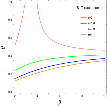
Figure 1: The $S$-$T$ bound on the parameter space at $99\%$ confidence level in the plane of $(\theta-\widetilde{g})$ for $r=0.1,0.6,0.9,1.1$, with the cut off scale $\Lambda=\sqrt{2}\pi v/\sin\theta$. The region above the curves is excluded by EWPT.

Additionally, deviations in the Higgs coupling w.r.t. the SM ones also bring additional contributions to the $S$ and $T$ parameters. The modification in the Higgs coupling, eq. (77), produce approximately the following deviations in the $S$ and $T$ parameters.

$$\Delta S = \frac{1}{6\pi}\left[(1-\kappa_{V}^{2})\log\left(\frac{\Lambda}{m_{h}}\right)+\log\left(\frac{m_{h}}{m_{h,ref}}\right)\right]\,,$$ (92)

$$\Delta T = -\frac{3}{8\pi\cos^{2}\theta_{W}}\left[(1-\kappa_{V}^{2})\ln\frac{\Lambda}{m_{h}}+\log\left(\frac{m_{h}}{m_{h,ref}}\right)\right]\,.$$ (93)

In the above formulas, the couplings of the SM gauge bosons to the Higgs, $\kappa_{V}$, include corrections up to order $1/\widetilde{g}^{2}$ from eq. (82) in order to be consistent with the tree-level effects (for simplicity, we neglect the term in ${g^{\prime}}^{2}$ so that $\kappa_{V}\sim\kappa_{W}\sim\kappa_{Z}$). In principle, the heavy resonances also contribute at one-loop level: naively, the loops with a Higgs boson have an additional suppression $1/\widetilde{g}^{2}\cdot m_{W}^{2}/M_{V}^{2}\sim 1/\widetilde{g}^{4}$. Pure loops of the heavy resonances may be unsuppressed, however their effect should be small as the dynamics is custodial invariant. Furthermore, due to the intrinsic strong interactions among resonances, such loop calculations are not reliable in general because perturbative expansions cannot be trusted. In this paper, therefore, we follow the philosophy of Vector Meson Dominance (which is experimentally tested in QCD) and assume that the tree level exchange is the dominant contribution, while effects due to loops or higher order operators can be neglected. Alternative proposals have been put forward in the literature in order to render the theory more calculable, see for instance Contino:2011np . The main idea is to assume that the lowest lying resonances are weakly coupled to themselves and the rest of the dynamics, so that loops can be reliably calculated, together with the assumption of negligible higher order operators. As a result, potential cancellations have been observed that can relax the constraints from EW precision tests Contino:2015mha ; Ghosh:2015wiz , including loop contributions from light top partners: these results, however, are not generic. Loop corrections can be considered a modelling of the contribution of the strong dynamics (see also Pich:2013fea ; Contino:2015gdp ). In principle, improved calculability in Ref. Contino:2011np can be imposed on our model, however we prefer to stay with a more conservative bound, as an order of magnitude estimate of the resonance effects.

The experimental values from PDG for $S$ and $T$ (leaving $U$ to be free), with a strong correlation coefficient $0.90$, at $1\sigma$ deviation are Agashe:2014kda :

$$S=-0.03\pm 0.10\,,\quad T=0.01\pm 0.12\,.$$ (94)

The corresponding limits on the model parameters are shown in fig. (1). For $r\gtrsim 1$ the vector partially cancels the Higgs contribution allowing a larger parameter space: in some areas of the parameter space, therefore, the most constraining bound comes form the measurements of the Higgs couplings, which give constraints on $\theta$ of the order of $\theta\lesssim 0.6$ Arbey:2015exa . Another effect that may significantly modify the EWPT is the presence of the $\sigma$ state, that will in general mix with $h$, with an un–calculable mixing angle $\alpha$, and can potentially alleviate the constraints from EWPT Arbey:2015exa .

IV A minimal fundamental gauge theory

The effective model characterised in the previous sections, can originate from a very simple scalar–less underlying theory Ryttov:2008xe ; Galloway:2010bp : it consists of a gauged and confining ${\cal G}_{\rm HC}=\mbox{SU(2)}$ with two light Dirac flavours transforming as the fundamental representation. Following the notation of Ryttov:2008xe ; Cacciapaglia:2014uja , the 2 Dirac fermions, $U$ and $D$, can be arranged in a flavour SU(4) multiplet as

$$Q_{\alpha}^{i,a}=\left(\begin{array}[]{c}U_{L}\\ D_{L}\\ \widetilde{U_{L}}\\ \widetilde{D_{L}}\end{array}\right),$$ (95)

where $\alpha$ is the spin Lorentz index, $i$ is a flavour index and $a$ is a hyper–colour index. The tilded fields are left-handed spinors containing the right-handed components of the Dirac fields, i.e. $\tilde{U}_{L}=-i\sigma^{2}U_{R}^{*}$ and $\tilde{D}_{L}=-i\sigma^{2}D_{R}^{*}$.

Following the embedding of the EW symmetry we chose in this work, the pair $(U_{L},D_{L})$ transforms as a doublet of the weak isospin SU(2)_L, while the other two $(\tilde{U}_{L},\tilde{D}_{L})$ as an anti-doublet of the custodial SU(2)_R.

IV.1 Scalar sector

The scalar sector of the $SU(4)/Sp(4)$ models was studied in Cacciapaglia:2014uja . In general we can write a scalar matrix

$$M_{ij}=Q^{\alpha A}_{i}Q_{\alpha Aj}=Q_{\beta Bi}Q_{\alpha Aj}I^{AB}\epsilon^{\alpha\beta}$$ (96)

where greek letters are Lorentz indices, capital letter are hyper–colour gauge indices and lower case latin are flavour indices. The gauge group invariant $I_{AB}$ depends on the gauge group and fermion representation. If the gauge representation is pseudo-real, like in our case, $I_{AB}$ is antisymmetric (for fundamentals of SU(2)_HC, $I^{AB}=\epsilon^{AB}$). Accordingly, $M$ is flavour anti-symmetric, and it transforms as a 6_SU(4). In general, this matrix contains both the light pNGBs and heavier scalar resonances.

IV.2 Vector sector

The composite spin-1 states can be defined in terms of the underlying fermions via the flavour adjoint left-current:

$$({\cal F}^{\mu})_{i}^{j} \sim \left(Q_{i}^{\alpha}\sigma^{\mu}_{\alpha\dot{\beta}}Q^{\dagger j\dot{\beta}}-\frac{1}{4}\delta_{i}^{j}\,Q_{k}^{\alpha}\sigma^{\mu}_{\alpha\dot{\beta}}Q^{\dagger k\dot{\beta}}\right)$$ (97)

$$= \left(Q_{i}^{\alpha a}\sigma^{\mu}_{\alpha\dot{\beta}}Q_{j}^{b\dagger\dot{\beta}}-\frac{1}{4}\delta_{ij}\,Q_{k}^{a\alpha}\sigma^{\mu}_{\alpha\dot{\beta}}Q_{k}^{b\dagger\dot{\beta}}\right)\mathcal{E}_{ab}$$ (98)

$$= -\left(Q_{j\dot{\alpha}}^{\dagger}\overline{\sigma}^{\mu}Q_{\beta i}-\frac{1}{4}\delta_{ij}\,Q_{k\dot{\alpha}}^{\dagger}\overline{\sigma}^{\mu}Q_{k\beta}\right)\mathcal{E}_{ab}$$ (99)

where $\mathcal{E}_{ab}$ is the antisymmetric tensor making a hyper-colour singlet. Note the first line is non-standard notation for the left bilinears, but the one that directly implements the the flavour transformation structure ${\cal F}\to g\cdot{\cal F}\cdot g^{\dagger}$. The last line is the standard bilinear notation. After some current algebra, the components in the vector matrix from tab. (1) can be associated to currents in terms of the underlying quarks, as detailed in tab. (2), where the notation is used: $\Re(J^{\mu})=\frac{1}{2}(J^{\mu}+J^{\mu{\dagger}})$ and $\Im(J^{\mu})=-\frac{i}{2}(J^{\mu}-J^{\mu{\dagger}})$.

Field	Fermion currents	P	C	G	GP
Massive spin-1 ${\cal V}_{\mu}$ (unbroken generators)
$v^{+}$	$\overline{D}\gamma^{\mu}U$
$v^{0}$	$\frac{1}{\sqrt{2}}\left(\overline{U}\gamma^{\mu}U-\overline{D}\gamma^{\mu}D\right)$	$-$	$-$	$-$	$+$
$v^{-}$	$\overline{U}\gamma^{\mu}D$
$\tilde{v}^{0}$	$\sqrt{2}\cos\theta\,\Im\left(U^{T}C\gamma^{\mu}D\right)+\frac{1}{\sqrt{2}}\sin\theta\,\left(\overline{U}\gamma^{\mu}U+\overline{D}\gamma^{\mu}D\right)$	$-$	$-$	$+$	$-$
$s^{+}$	$\cos\theta\,\left(\overline{D}\gamma^{\mu}\gamma^{5}U\right)+\frac{i}{2}\sin\theta\,\left(U^{T}C\gamma^{\mu}\gamma^{5}U-\overline{D}\gamma^{\mu}C\gamma^{5}\overline{D}^{T}\right)$
$s^{0}$	$-\frac{1}{\sqrt{2}}\cos\theta\,\left(\overline{U}\gamma^{\mu}\gamma^{5}U-\overline{D}\gamma^{\mu}\gamma^{5}D\right)-\sqrt{2}\sin\theta\,\Im\left(U^{T}C\gamma^{\mu}\gamma^{5}D\right)$	$+$	$+$	$+$	$+$
$s^{-}$	$\cos\theta\,\left(\overline{U}\gamma^{\mu}\gamma^{5}D\right)+\frac{i}{2}\sin\theta\,\left(\overline{U}\gamma^{\mu}C\gamma^{5}\overline{U}^{T}-D^{T}C\gamma^{\mu}\gamma^{5}D\right)$
$\tilde{s}^{+}$	$\frac{i}{2}\left(U^{T}C\gamma^{\mu}\gamma^{5}U+\overline{D}\gamma^{\mu}C\gamma^{5}\overline{D}^{T}\right)$
$\tilde{s}^{0}$	$\sqrt{2}\,\Re\left(U^{T}C\gamma^{\mu}\gamma^{5}D\right)$	$+$	$-$	$-$	$-$
$\tilde{s}^{-}$	$\frac{i}{2}\left(\overline{U}\gamma^{\mu}C\gamma^{5}\overline{U}^{T}+D^{T}C\gamma^{\mu}\gamma^{5}D\right)$
Massive spin-1 ${\cal A}_{\mu}$ (broken generators)
$a^{+}$	$\frac{i}{2}\cos\theta\,\left(U^{T}C\gamma^{\mu}\gamma^{5}U-\overline{D}\gamma^{\mu}C\gamma^{5}\overline{D}^{T}\right)-\sin\theta\,\left(\overline{D}\gamma^{\mu}\gamma^{5}U\right)$
$a^{0}$	$-\sqrt{2}\cos\theta\,\Im\left(U^{T}C\gamma^{\mu}\gamma^{5}D\right)+\frac{1}{\sqrt{2}}\sin\theta\,\left(\overline{U}\gamma^{\mu}\gamma^{5}U-\overline{D}\gamma^{\mu}\gamma^{5}D\right)$	$+$	$+$	$+$	$+$
$a^{-}$	$\frac{i}{2}\cos\theta\,\left(\overline{U}\gamma^{\mu}C\gamma^{5}\overline{U}^{T}-D^{T}C\gamma^{\mu}\gamma^{5}D\right)-\sin\theta\,\left(\overline{U}\gamma^{\mu}\gamma^{5}D\right)$
$x^{0}$	$\sqrt{2}\,\Re\left(U^{T}C\gamma^{\mu}D\right)$	$-$	$+$	$-$	$+$
$\tilde{x}^{0}$	$\frac{1}{\sqrt{2}}\cos\theta\,\left(\overline{U}\gamma^{\mu}U+\overline{D}\gamma^{\mu}D\right)-\sqrt{2}\sin\theta\,\Im\left(U^{T}C\gamma^{\mu}D\right)$	$-$	$-$	$+$	$-$

Table 2: Classification of composite vectors in terms of the underlying fermionic currents, using a notation $C=\gamma^{0}\gamma^{2}$. We quote transformation properties in terms of spacial parity P, charge conjugation C, and pion parity G defined from listed currents. The combination GP is a good symmetry from the strong dynamics. In our notation, P-parity is defined in spacial direction, i.e. $(-1)^{\mu}$ is “$-$” parity.

Field	Fermion currents	$P$	$C$	$G$	$GP$
Scalar pNGBs
$h$	$\frac{1}{2}\cos\theta\,\left(\overline{U}U+\overline{D}D\right)+\sin\theta\,\Im\left(U^{T}CD\right)$	$+$	$+$	$+$	$+$
$\eta$	$\Re\left(U^{T}CD\right)$	$+$	$-$	$-$	$-$

Table 3: Classification of the pNGB states in terms of the underlying fermionic currents, and their parities.

We first notice that this decomposition matches with the interpretation we provided at the beginning of the previous section: the triplet $\overrightarrow{v}_{\mu}$ corresponds to the “vector” current $\bar{Q}\gamma_{\mu}Q$, typically associated to the $\rho_{\mu}$ meson in QCD, while $\overrightarrow{s}_{\mu}$ and $\overrightarrow{a}_{\mu}$ contain an “axial” current component, associated with $a_{\mu}$ meson in QCD, proportional to the $\cos\theta$ and $\sin\theta$ respectively. More precisely, due to the symmetry relating the Technicolor limit to the composite Higgs limit, the $\cos\theta$ component of $s_{\mu}^{\pm,0}$ and $\tilde{x}_{\mu}^{0}$ can be exactly mapped from the $\sin\theta$ component of $a_{\mu}^{\pm,0}$ and $\tilde{v}_{\mu}^{0}$.

IV.3 Discrete symmetries

The action of space-time discrete symmetries on the composite states can be derived from the transformation properties of the underlying quarks. However, the gauging of the EW interactions break $P$ and $C$ individually, but preserves $CP$ in the strong confining sector. Under $CP$, the bound state fields transform as

$$M\xrightarrow{CP}M^{\dagger}\,,\qquad{\cal F}_{\mu}\xrightarrow{CP}-(-1)^{\mu}({\cal F}_{\mu})^{T}\,,$$ (100)

where $(-1)^{\mu}=1$ for $\mu=0$, and $-1$ on spacial directions. The parities associated with the spin–1 resonances are summarised in tab. (2): in our notation, a vector has $CP=+$, while $CP=-$ for a pseudo-vector. In the scalar sector, as expected, the Higgs $h$ is defined as a scalar, while $\eta$ transforms as a pseudo-scalar, see tab. (3).

However, $CP$ is not a convenient symmetry to label states as it maps charged states in their complex conjugate (particles into anti-particles). In terms of composite states, it is thus convenient to define a new parity $G$, defined as $C$ plus an internal rotation in the flavour symmetry, which corresponds to an SU(2) rotation in our case:

$$U\xrightarrow{G}-\gamma^{2}D^{\ast}\,,\qquad D\xrightarrow{G}\gamma^{2}U^{\ast}\,.$$ (101)

with its action on fermion current illustrated in appendix B. Once combined with $P$, the new symmetry defines a parity acting as:

$$M\xrightarrow{GP}\Omega_{GP}\cdot M^{\dagger}\cdot\Omega_{GP}^{T}\,,\quad{\cal F}_{\mu}\xrightarrow{GP}(-1)^{\mu}\Omega_{GP}\cdot({\cal F}_{\mu})^{T}\cdot\Omega_{GP}\,,\quad\Omega_{GP}=\left(\begin{array}[]{cc}\sigma^{2}&0\\ 0&\sigma^{2}\end{array}\right)\,.$$ (104)

From tab. (2) and tab. (3) we see that all the tilded fields are odd under $GP$, as well as $\eta$, thus this is the symmetry preventing decays of such field directly into SM ones. Note, however, that $GP$ is violated by the anomalous WZW term which generates decays for $\eta$. Additional decay channels will also be generated for the vectors.

V Phenomenology at the LHC and future 100 TeV colliders

V.1 Model implementation

To study the phenomenology of this model, we implemented the Lagrangian in MadGraph Alwall:2014hca , using the Mathematica package FeynRules Alloul:2013bka . The implementation of the FeynRules model file is sketched in this section, while the model files are publicly available on the HEPMDB website .

The neutral resonances $A$, $Z$, $A^{0}$, $V^{0}$, $S^{0}$, $\tilde{S}^{0}$ and $\tilde{V}^{0}$ are introduced as one particle class of VN, with two additional neutral states $X^{0}$, $\tilde{X}^{0}$ into another particle class of VX. The charged resonances $W^{+}$, $A^{+}$, $V^{+}$, $S^{+}$ and $\tilde{S}^{+}$ are put into one particle class of VC. The effective Lagrangian for the strong sector is written in terms of physical pions, thus in the Unitary gauge, and vector bosons in gauge basis, with the latter rotated to their mass eigenstates via mixing matrices. The quarks and leptons only couple to $\widetilde{W}$ and $B$, thus the Yukawa structure is exactly the same as in the Standard Model. In the model implementation, the rotation matrices CM_4×4 and NM_5×5 are provided in two independent Les Houches blocks of VCMix and VNMix as external parameters, whose numerical values are calculated by a specific Fortran routine. Note that for the rotation, the eigenstates are ordered such that the diagonal element in CM_4×4 or NM_5×5 are maximal in each corresponding column, to make sure each one carries the largest component of the original gauge state as described in eq. (59).

Five model parameters $M_{V}$, $M_{A}$, $r$, $\theta$ and $\widetilde{g}$ are introduced into the Les Houches block DEWSB, with all associated decay constants $f_{1}=\sqrt{2}M_{A}/\widetilde{g}$, $f_{K}=\sqrt{2}M_{V}/\widetilde{g}$ and $f_{0}=\sqrt{v^{2}/\sin^{2}\theta+f_{1}^{2}r^{2}}$ defined as internal parameters in the model file. Note that the latter relation derives directly from fixing the value of $G_{F}$ (i.e. the EW scale $v$), as shown in eq. (69). Furthermore, we have imposed the SM values of $e$ and $M_{Z}$ into the following analytic expressions to calculate $g^{\prime}$ and $g$ in terms of the independent model parameters.

$$\frac{1}{e^{2}}=\frac{1}{g^{\prime 2}}+\frac{1}{g^{2}}+\frac{2}{\widetilde{g}^{2}}\,,\quad\det\left(M_{N}^{2}-M_{Z}^{2}I_{5}\right)=0$$ (105)

The model file is loaded using FeynRules package which exports the Lagrangian into UFO format Degrande:2011ua . We implement one python code as the parameter card calculator, to conduct the numerical rotation and write all block information into a param_card.dat.

V.2 LHC Run–II

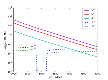
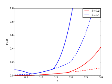
a)	b)

Figure 2: Left: Drell–Yan cross section of composite states for $M_{A}=3\mbox{ ${\mathrm{TeV}}$}$, $\widetilde{g}=3.0$, $r=0.6$ and $\theta=0.2$ at LHC Run–II with $\sqrt{s}=13\mbox{ ${\mathrm{TeV}}$}$. Right: The largest $\Gamma/M$ of composite resonances as a function of $r$, with $M_{V}=2.5$ TeV, $M_{A}=3$ TeV, $\widetilde{g}=3.0$   (solid line) and $\widetilde{g}=6.0$ (dashed line).

At the LHC Run–II, several resonances may be produced via the Drell-Yan production mechanism, with $qq^{\prime}$ as initial states, therefore unfolding a delighting and rich phenomenology just like hadron spectroscopy in QCD but with completely new challenges and opportunities. Here we briefly discuss what would be the first probable observations in the vector sector of our model, by investigating cross sections and experimental bounds from a $\sqrt{s}=$13 TeV LHC. The calculation is conducted in MadGraph 5 Alwall:2014hca , using the PDF set NN23LO Ball:2012cx .

We present the cross section for each resonance at the LHC Run II in fig. (2)a by varying the parameter of $M_{V}$, with fixed $M_{A}=3\mbox{ ${\mathrm{TeV}}$}$, $r=0.6$ and $\theta=0.2$. The leading production channel is for the resonance $V^{\pm}$, followed by the neutral resonances $V^{0}$ and $S^{0}$. The vector resonance $S^{\pm}$ is defined as the one with largest portion of $s^{+}$ state, with exact mass of $M_{V}$. This state is rotated out from the matrix ${\cal{C}}^{a}$ in eq. (128), as a linear combination of $v^{+}$ and $s^{+}$, thus it can not be directly produced due to current model set up. Increasing $\widetilde{g}$ will result in a smaller cross section as the couplings to quarks, generated by the mixing, are suppressed. Furthermore, only $\sigma_{A^{\pm,0}}$ shows clear dependence on the other parameters, $\theta$ and $r$, and in the case of $M_{V}<M_{A}$, $\sigma_{A^{\pm,0}}$ will always be subleading to $\sigma_{V^{\pm,0},S^{0}}$ by several orders of magnitude. Note that for the “axial” resonances $A^{\pm}$ and $A^{0}$, the cross sections turn out to be zero at the point of $M_{V}=M_{A}$, since the mixing does not contain any component of $\widetilde{W}$ and $B$ and they decouple from SM quarks. We also check the parameter space where the narrow width approximation (NWA) can be used, as shown in fig. (2)b where we find that the relevant parameter is $r$. We set the benchmark point to be $M_{V}=2.5$ TeV and $M_{A}=3$ TeV, and vary the other parameters $(\widetilde{g},\theta,r)$ to inspect the region where the largest $\Gamma/M$ among all resonances is less than $50\%$. Generally, in order to use NWA as an approximate analysis for the event line shapes (e.g. di-lepton invariant mass distribution) we require $\Gamma/M<10\%$ so that interference effects with $Z,\gamma$ can be safely neglected. Due to the small mass split between many resonances, off-diagonal width effects may also be important Cacciapaglia:2009ic ; deBlas:2012qp . Furthermore, the small width region will be favoured in order to resolve the compressed multi-peaking structure in the spectrum. According to this criterion, for a small $\theta=0.2$, the NWA applies very well for $0<r<2.0$, but with a larger value $\theta=0.4$, the resonance will become broad and we need at least to tune $\widetilde{g}>6.0$ for the NWA to be effective.

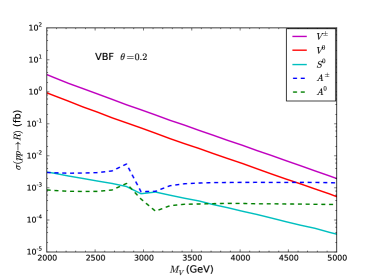
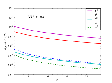
Figure 3: Vector Boson Fusion (VBF) cross sections of composite states for $M_{A}=3\mbox{ ${\mathrm{TeV}}$}$, $r=0.6$ and $\theta=0.2$ at LHC Run–II with $\sqrt{s}=13\mbox{ ${\mathrm{TeV}}$}$. On the left: $\widetilde{g}=3.0$ is fixed and $M_{V}$ varies; On the right: $M_{V}=2.5\mbox{ ${\mathrm{TeV}}$}$ and $\widetilde{g}$ varies.

Alternatively the composite resonances can be produced via vector boson fusion (VBF)Belyaev:2008yj ; Franzosi:2012ih ; Mohan:2015doa , with the production cross sections shown in fig. (3) for the same benchmark scenario. In the calculation for $pp\to R$+2 jets ($R=A^{0,\pm},V^{0,\pm},S^{0}$), we consider all pure EW diagrams which form a gauge invariant set with the VBF topology, including diagrams with one $t$-channel weak boson exchange following a composite resonance emitted from a quark line. Although the signal definition is ambiguous we expect that the VBF topology dominates. It was required $p_{T}(j)>20$ GeV in order to avoid the $t$-channel singularity of a photon exchange. The longitudinal weak bosons, $W_{L}$, coupled to composite vectors through partial compositeness, play a less important role due to small mixing angles. This is noticed that in the right hand panel of fig. (3), the cross section decreases with $\widetilde{g}$. Therefore, in general VBF is a subdominant production mechanism. As previously remarked in Belyaev:2008yj , the exception to this trend occurs in the special parameter space region $M_{A}\simeq M_{V}$, where the Drell–Yan production of $A^{0,\pm}$ is highly suppressed.

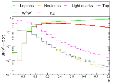
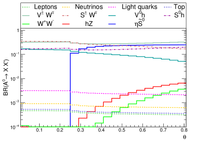
(a)	(b)
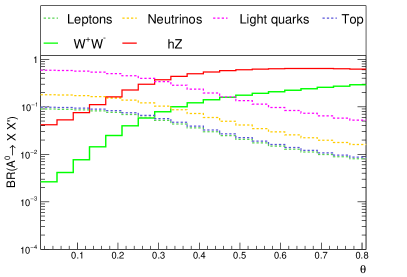
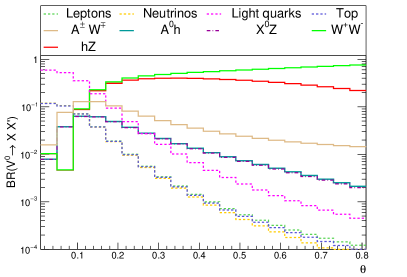
(c)	(d)

Figure 4: Branching ratios (BR) of composite states $V^{0}$ and $A^{0}$, with the dependence on $\theta$ for $\widetilde{g}=3.0$, $r=0.6$, $M_{V}=2.5$ TeV (top row) and $M_{V}=3.5$ TeV (bottom row), with fixed $M_{A}=3$ TeV.

In fig. (4), we show the typical branching ratios for $V_{0}$ and $A_{0}$, with all the decays into SM fermions drawn in dotted line ($V^{+},\,A^{+}$ show similar decay pattern). The entry in the legend is well patterned, each mode arranged in the same colour and line-style in order to easily compare the differences in each scenario, with top standing for $t\bar{t}$, light quarks for $u_{1,2}\bar{u}_{1,2}$+$d_{1,2}\bar{d}_{1,2}$ (Cabibbo CKM mixing used), leptons for $l^{+}l^{-}$ and neutrino for $\nu\bar{\nu}$. For the decay of $A^{0}$ in the case of $M_{V}<M_{A}$, we draw the mode with $V^{\pm,0}$ in the solid line while the mode with $S^{\pm,0}$ is in the dash-dotted line, since there is certain overlap between the decay modes of $V^{0}h$ and $S^{0}h$, similar for $V^{\pm}W^{\mp}$ and $S^{\pm}W^{\mp}$, in the low $\theta$ region, but start to split from $\theta\gtrsim 0.3$. An analogous situation happens to the decay of $V^{0}$ in the case of $M_{A}<M_{V}$, where branching ratios into $A^{0}Z$ and $X^{0}h$, mostly overlap with each other in the range of $0<\theta<0.8$ due to the global symmetry. We also explore the branching ratios as a function of $r$: the fermions spectrum goes to a maximum at $r=1$, while the $WW$ or $hZ$ spectrum, instead, goes to a minimum since the coupling is $\propto(r^{2}-1)$ at $1/\widetilde{g}$ order. In either vector or axial resonance dominant case, the lower mass state displays a larger branching ratio into $l^{+}l^{-}$ and $W^{+}W^{-}$ rather than into final states containing a composite vector, therefore we can exploit the most recent LHC Run–II results to constrain the model parameters.

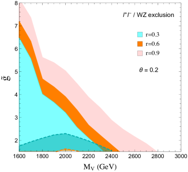
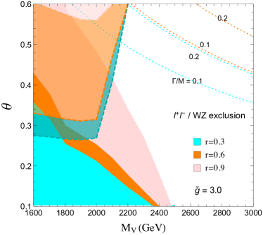
Figure 5: Excluded region with $M_{V}=M_{A}$, recast from the $95\%$ observed limit for the di-lepton $l^{+}l^{-}$ and di-boson $WZ$ channel measured by ATLAS at LHC Run–II. The $l^{+}l^{-}$ exclusion is in solid lines, and the $WZ$ exclusion in dashed ones. The parameter $r$ is varied in the range of $[0,1]$, with contours in the $(\widetilde{g}-M_{V})$ plane on the left and in the $(\theta-M_{V})$ plane on the right. The region with $\Gamma/M>0.1$, where NWA is not applicable, is identified by dotted contour lines.

Since our model provides several candidates as a heavy $Z^{\prime}$ or $W^{\prime}$, the LHC measurement for the Drell-Yan process and di-boson process would impose a stringent constraint on the parameter space. We calculate the theoretical cross section for $pp\to R^{0}\to l^{+}l^{-}$ and $pp\to R^{\pm}\to WZ$ in this $SU(4)/Sp(4)$ model and compare them with the $95\%$ upper bound observed from the latest ATLAS measurement dilepton ; diboson . Similar results can be obtained by using the corresponding CMS searches CMS:2015nhc ; CMS:2015nmz . The single lepton plus MET process is expected to require similar constraints to the di-lepton ones, thus we do not consider the $l\nu$ channel in detail for simplicity. We derive the exclusion limits in the parameter space specified by ($\widetilde{g}$, $\theta$, $r$ ) after assuming $M_{V}=M_{A}$. Since we have not included the acceptance factor into this analysis, our result would be stronger than the exact $95\%$ exclusion from the LHC Run–II searches. We show the exclusion contours from $l^{+}l^{-}$ and $WZ$ in fig. (5), with the di-lepton bound drawn in solid line, and the di-boson bound in dashed line. The plot shows that the two channels are complementary to each other. Notice that for an increasing $r$ (in range of $[0,1]$), the di-lepton channel imposes a stronger exclusion limit than the di-boson. The left panel of fig. (5) shows that the lower limit for the mass of the resonances approaches $M_{V}\gtrsim 2.5$ TeV for a coupling constant $\widetilde{g}\simeq 3.0$ and small angle $\theta=0.2$. The right panel of fig. (5) also shows that the di-lepton limit is more sensitive to the small $\theta$ area, while the di-boson channel mainly probes the large $\theta$ area. To summarise, for small $\theta<0.2$, as expected in composite pNGB Higgs limit of the model Arbey:2015exa , the di-lepton searches impose a lower bound on $M_{V}$ between $2$ and $2.5$ TeV, depending on the value of $r$.

V.3 Future 100 TeV proton colliders

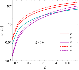
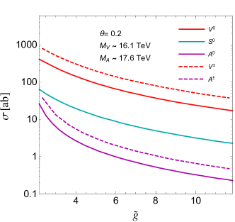
(a)	(b)
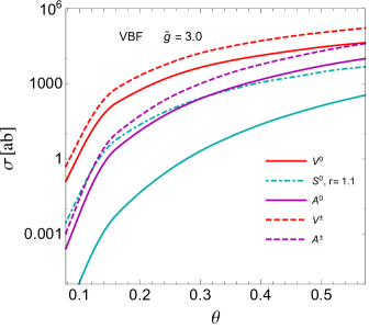
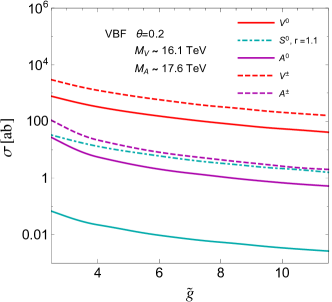
(c)	(d)

Figure 6: Drell-Yan ( plots (a) and (b) ) and Vector Boson Fusion ( plots (c) and (d) ) cross sections of composite states with $M_{V}=3.2/\sin(\theta)$ TeV, $M_{A}=3.5/\sin(\theta)$ TeV at $\sqrt{s}=100\mbox{ ${\mathrm{TeV}}$}$. The left panel shows the dependence on $\theta$ for $\widetilde{g}=3.0$, $r=1.0$. The right panel shows the dependence on $\widetilde{g}$ for $r=1.0$ and $\theta=0.2$. For the $S^{0}$ VBF production, the dot-dashed cyan line is using $r=1.1$, compared with the solid cyan line of $r=1.0$.

As shown in the previous section, current LHC bounds on the resonances range in the $2$ TeV ballpark. However, the naive expectation is that the resonances populate this mass range only in the Technicolour limit, where $f_{\pi}\sim v$, in the composite pNGB limit, all the resonances’ masses would be enhanced by a factor $1/\sin\theta$ due to the increase in the compositeness scale. Thus, the most natural mass range seem to lie above tens of TeV, thus more relevant for a future 100 TeV collider than for the LHC. For the simplest underlying gauge theory realising $SU(4)/Sp(4)$ global symmetry, namely $SU(2)$ with 2 Dirac fermions, lattice results have recently been published Arthur:2016dir , providing a first numerical prediction for the masses of the spin-1 resonances, found to be $M_{A}=3.5\mbox{ ${\mathrm{TeV}}$}/\sin(\theta)$ and $M_{V}=3.2\mbox{ ${\mathrm{TeV}}$}/\sin(\theta)$, far from LHC reach in the small $\theta$ limit. Thus, a machine colliding protons at $\sqrt{s}=100\mbox{ ${\mathrm{TeV}}$}$ would be a perfect stage to probe its vast spectrum. It should be noted, however, that the masses can be lighter in different underlying gauge theories. In such case, even though the mass scales as $1/\sin\theta$, the resonances might be at the reach of LHC.

The Drell-Yan production of the states $V^{0,\pm}$, $S^{0}$ and $A^{0,\pm}$ are shown in the top row of fig. (6) as functions of $\theta$ and $\widetilde{g}$. When we use Madgraph for simulation, only the PDF of the first two generations of quarks are taken into account. However, at the high energy collider, the top and bottom quark PDFs can be important and need to be included to conduct a reliable prediction at 100 TeV Han:2014nja . Nonetheless, the cross sections present here can serve as a guideline. Similarly to the scenario described in the last section, the production rate for these states with $r\sim 1$ is not large, around ${\cal{O}}(1)$ fb for $\theta\sim 0.2$, since the resonance coupling to SM quarks are generated via mixing.

At 100 TeV, Vector Boson Fusion plays a more important role due to the enhancement of collinear radiated weak bosons from the spectator quarks, which translates into a large effective luminosity of weak bosons inside the proton in the language of the Effective W approximation Chanowitz:1985hj . Indeed, the importance of VBF can be appreciated in the bottom row of fig. (6), which shows that for $V^{0,\pm}$ and $A^{0,\pm}$ resonances the VBF cross section is dominant over the Drell–Yan production, with very mild dependence on $r$. However the $S^{0}$ production is much more sensitive to $r$. Since the $W^{+}W^{-}S^{0}$ coupling almost vanishes at the point of $r=1.0$, with the main contribution to VBF from the $V^{\pm}W^{\mp}S^{0}$ fusion, this makes the $S^{0}$ production particularly small. But once departing from $r=1.0$, the $W^{+}W^{-}S^{0}$ fusion turns back to be important, therefore the VBF cross section for $S^{0}$ is actually two orders of magnitude larger in the case of $r=1.1$.

It is also important to note that SM physics, jets, top production and other important background for the process will present quite peculiar aspects at a 100 TeV collider (see e.g. Bothmann:2016loj ) and must be taken into consideration for a more precise phenomenological analysis.

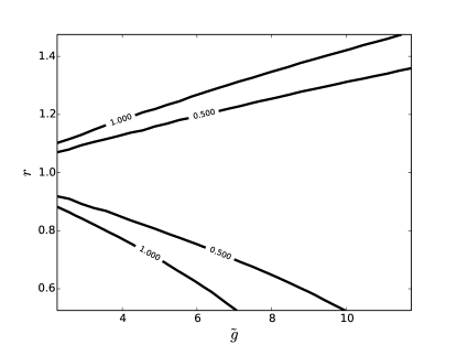
Figure 7: The largest ratio of width over mass $max(\Gamma_{R}/M_{R})$ among all the resonances. For large $r$, some resonances become too broad. The value of $\theta$ is set to 0.2, and the dependence on $\theta$ is very small in the perturbative region.

The value of $r$ is constrained by perturbativity of the effective description. The consistent region is illustrated in fig. (7), with the largest ratio of width over mass extracted in the plane of $(\widetilde{g}-r)$. We find that the region of $r$ close to one is where all the resonances are narrow, thus it is valid to apply the NWA for event analysis. For $r\neq 1$ the coupling of heavy vector to longitudinal bosons rapidly grows as the width of the resonance approaches its mass, jeopardising perturbativity and the validity of the description Bando:1987br .

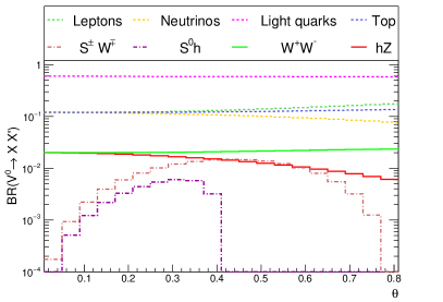
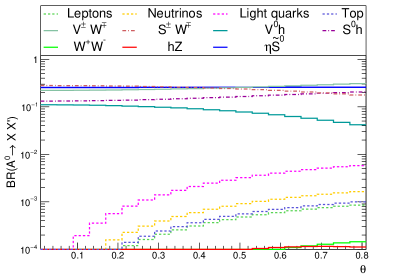
(a)	(b)
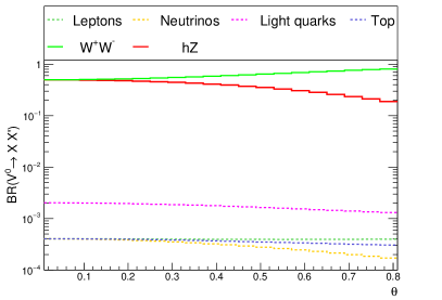
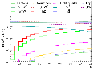
(c)	(d)

Figure 8: Branching ratios (BR) of composite states $A_{0}$ and $V_{0}$, with the dependence on $\theta$ for $M_{V}=3.2/\sin(\theta)$ TeV, $M_{A}=3.5/\sin(\theta)$ TeV, $\widetilde{g}=3.0$ and $r=1.0$ (top row) and $r=1.1$ (bottom row).

We show the BR of $V^{0}$ state as a function of $\theta$ in the left panel of fig. (8). $S^{0}$ has similar decay structure as $V^{0}$, while charged states present similar pattern, thus we do not show them here. At $r=1$ they mainly decay into SM fermions, in particular into di-jets. There will be small differences in the BR spectrum between $V^{0}$ and $S^{0}$. We find that, in the channel of di-leptons, $V_{0}$ decays at $\sim 10\%$ and $S_{0}$ at $\sim 40\%$. Moreover, for $V_{0}$, the decay into $W^{+}W^{-}$ is larger than $hZ$, while for $S_{0}$ the decay of $hZ$ turns to dominate over $W^{+}W^{-}$. Varying $r$ to be slightly larger than $1$, notable changes happen as the di-boson and $hZ$ channels rapidly overcome the fermion ones. For $r=1.1$ the branching ratios are close to $45\%$, equally split between $W^{+}W^{-}$ and $hZ$ at small $\theta$. Only small variation can be observed in $\theta\gtrsim 0$, but the two channels will start to split exactly till $\theta\lesssim 0.8$.

The decay pattern of the $A_{0}$ resonance is shown in the right panel of fig. (8), with more channels opened. At $r=1$, the fermion channel is subdominant, while the $WW$, $hZ$ channels almost disappear. The decay into $V^{\pm}/S^{\pm}W^{\mp}$ and $V^{0}/S^{0}h$ become competitive, and we can observe dominant decays into $\eta\tilde{S}$, with $\eta$ further decaying into a pair of tops, or gauge bosons via the WZW anomaly term (as discussed in Arbey:2015exa ). Since the $\tilde{S}$ decay is nearly $100\%$ to $Z\eta$ for the lattice benchmark point, this will give rise to novel collider signature of $4t+Z$ final states. For $r=1.1$ the di-boson and Higgs-strahlung channels enter into play, but this does not alter the picture dramatically.

It has been argued that the luminosity of this future machine should be at least a factor 50 larger than the LHC luminosity in order to profit from its full potential to find new physics Richter:2014pga ; Rizzo:2015yha . An integrated luminosity of $3-30~{}ab^{-1}$ per year is therefore expected, leading to several heavy vector bosons produced and a promising phenomenology. We also stress that probing masses up to $\sim 50$ TeV indirectly tests the models at small values of $\theta\sim 0.05$, where the high level of fine tuning renders the models unnatural and unappealing. While an ultimate exclusion is not possible due to a decouplings limit $\theta\to 0$ (like in supersymmetry), in our opinion a 100 TeV collider can ultimately probe the “motivated” region of the parameter space in this class of composite Higgs models.

VI Conclusions

In the present work we construct an effective Lagrangian that allows to describe vector spin-1 resonances in composite models of the Higgs boson. The framework adopted is the one of the hidden gauge symmetry approach, and we focus on a case with global symmetry structure based on the minimal case of an SU(4) symmetry broken to Sp(4). The chosen coset both satisfies the requirement of a custodial Higgs sector and allows for a fundamental composite description of the new resonances in terms of fermionic bound states. The SU(4) structure is promoted to SU(4)${}_{0}\times$SU(4)₁ in order to apply the hidden gauge symmetry idea and to obtain the vector and axial-vector states in the adjoint of the second SU(4). The paper discusses in detail the effective Lagrangian for these states and their properties including mass matrices, mixing and couplings. The underlying fundamental realisation of the theory in terms of fermionic bound states is also discussed, together with the associated discrete symmetries, such as parity.

Schematically, the model contains 3 triplets that mix with the standard model gauge bosons, plus additional states that do not mix. Therefore, the phenomenology is much richer than in the minimal case containing just a single isospin triplet. We outline the main properties of the spin-1 states and their role in the phenomenology of the basic model. At the LHC, the most sensitive channel for searching for the new resonances is di-lepton, which already imposes a bound on their mass around 2 TeV. The unmixed states, on the other hand, tend to decay into the singlet pion, $\eta$, thus providing new signatures compared to the minimal cases studied in the literature. Furthermore, in the case of a pseudo-Goldstone Higgs, where the compositeness scale is raised, the masses are expected to be higher, in the 10 TeV range. We show that a future 100 TeV collider may be able to probe the most interesting parameter space for naturalness. We focus on a minimal underlying description, where the masses have been computed on the Lattice, and detail the cross sections and branching ratios. This scenario can thus be one of the benchmark models for the 100 TeV collider.

This overview of the model, and its phenomenology, that we present is a template for the study of fundamental strong dynamics in the electroweak sector. Besides the specific case under study, which corresponds to the minimal fundamental model, it can be applied to other scenarios like, for instance, the case of composite strongly interacting Dark Matter candidates.

Appendix A Explicit formulas

The explicit embedding of the vectors in SU(4) matrix form, in terms of charge eigenstates (see tab. (1)), is

$$\bm{\mathcal{F}}_{\mu}\equiv\bar{\bm{\mathcal{F}}}_{\mu}+\widetilde{\bm{\mathcal{F}}}_{\mu}\,,$$ (106)

with

$$\bar{\bm{\mathcal{F}}}_{\mu}=\begin{pmatrix}{\displaystyle\frac{s_{\theta}a^{0}-c_{\theta}s^{0}+v^{0}}{2\sqrt{2}}}&{\displaystyle\frac{c_{\theta}s^{+}-s_{\theta}a^{+}+v^{+}}{2}}&{\displaystyle\frac{c_{\theta}a^{+}+s_{\theta}s^{+}}{2}}&{\displaystyle\frac{c_{\theta}a^{0}+s_{\theta}s^{0}-ix^{0}}{2\sqrt{2}}}\\ \vskip 3.0pt plus 1.0pt minus 1.0pt\\ {\displaystyle\frac{-s_{\theta}a^{-}+c_{\theta}s^{-}+v^{-}}{2}}&{\displaystyle\frac{c_{\theta}s^{0}-s_{\theta}a^{0}-v^{0}}{2\sqrt{2}}}&{\displaystyle\frac{c_{\theta}a^{0}+s_{\theta}s^{0}+ix^{0}}{2\sqrt{2}}}&{\displaystyle\frac{-c_{\theta}a^{-}-s_{\theta}s^{-}}{2}}\\ \vskip 3.0pt plus 1.0pt minus 1.0pt\\ {\displaystyle\frac{c_{\theta}a^{-}+s_{\theta}s^{-}}{2}}&{\displaystyle\frac{c_{\theta}a^{0}+s_{\theta}s^{0}-ix^{0}}{2\sqrt{2}}}&{\displaystyle-\frac{c_{\theta}s^{0}-s_{\theta}a^{0}+v^{0}}{2\sqrt{2}}}&{\displaystyle\frac{-s_{\theta}a^{-}+c_{\theta}s^{-}-v^{-}}{2}}\\ \vskip 3.0pt plus 1.0pt minus 1.0pt\\ {\displaystyle\frac{c_{\theta}a^{0}+s_{\theta}s^{0}+ix^{0}}{2\sqrt{2}}}&{\displaystyle\frac{-c_{\theta}a^{+}-s_{\theta}s^{+}}{2}}&{\displaystyle\frac{-s_{\theta}a^{+}+c_{\theta}s^{+}-v^{+}}{2}}&{\displaystyle\frac{c_{\theta}s^{0}-s_{\theta}a^{0}+v^{0}}{2\sqrt{2}}}\end{pmatrix}\ ,$$ (107)

$$\widetilde{\bm{\mathcal{F}}}_{\mu}=\begin{pmatrix}{\displaystyle\frac{s_{\theta}\widetilde{v}^{0}+c_{\theta}\widetilde{x}^{0}}{2\sqrt{2}}}&0&{\displaystyle\frac{\tilde{s}^{+}}{2}}&{\displaystyle\frac{c_{\theta}\widetilde{v}^{0}-s_{\theta}\widetilde{x}^{0}+i\widetilde{s}^{0}}{2\sqrt{2}}}\\ \vskip 3.0pt plus 1.0pt minus 1.0pt\\ 0&{\displaystyle\frac{c_{\theta}\widetilde{x}^{0}+s_{\theta}\widetilde{v}^{0}}{2\sqrt{2}}}&{\displaystyle\frac{-c_{\theta}\widetilde{v}^{0}+s_{\theta}\widetilde{x}^{0}+i\widetilde{s}^{0}}{2\sqrt{2}}}&{\displaystyle\frac{\widetilde{s}^{-}}{2}}\\ \vskip 3.0pt plus 1.0pt minus 1.0pt\\ {\displaystyle\frac{\widetilde{s}^{-}}{2}}&{\displaystyle\frac{-c_{\theta}\tilde{v}^{0}+s_{\theta}\widetilde{x}^{0}-i\widetilde{s}^{0}}{2\sqrt{2}}}&{\displaystyle-\frac{c_{\theta}\widetilde{x}^{0}+s_{\theta}\widetilde{v}^{0}}{2\sqrt{2}}}&0\\ \vskip 3.0pt plus 1.0pt minus 1.0pt\\ {\displaystyle\frac{c_{\theta}\widetilde{v}^{0}-s_{\theta}\widetilde{x}^{0}-i\widetilde{s}^{0}}{2\sqrt{2}}}&{\displaystyle\frac{\widetilde{s}^{+}}{2}}&0&{\displaystyle\frac{-c_{\theta}\widetilde{x}^{0}-s_{\theta}\widetilde{v}^{0}}{2\sqrt{2}}}\end{pmatrix}\ .$$ (108)

In the gauge eigenbasis, the vector mass matrices in the charged ${\cal M}_{\rm C}$ and neutral ${\cal M}_{\rm N}$ sectors are

$${\bf{\cal M}_{\rm C}^{2}}=\begin{pmatrix}{\displaystyle\frac{g^{2}M_{V}^{2}(1+\omega s_{\theta}^{2})}{\widetilde{g}^{2}}}&{\displaystyle\frac{-grM_{A}^{2}s_{\theta}}{\sqrt{2}\widetilde{g}}}&{\displaystyle\frac{-gM_{V}^{2}}{\sqrt{2}\widetilde{g}}}&{\displaystyle\frac{-gM_{V}^{2}c_{\theta}}{\sqrt{2}\widetilde{g}}}\\ {\displaystyle\frac{-grM_{A}^{2}s_{\theta}}{\sqrt{2}\widetilde{g}}}&{\displaystyle M_{A}^{2}}&0&0\\ {\displaystyle\frac{-gM_{V}^{2}}{\sqrt{2}\widetilde{g}}}&0&{\displaystyle M_{V}^{2}}&0\\ {\displaystyle\frac{-gM_{V}^{2}c_{\theta}}{\sqrt{2}\widetilde{g}}}&0&0&{\displaystyle M_{V}^{2}}\\ \end{pmatrix}\ ,$$ (109)

$${\bf{\cal M}_{\rm N}^{2}}=\begin{pmatrix}{\displaystyle\frac{g^{\prime 2}M_{V}^{2}(1+\omega s_{\theta}^{2})}{\tilde{g}^{2}}}&{\displaystyle-\frac{g^{\prime}gM_{V}^{2}\omega s_{\theta}^{2}}{\tilde{g}^{2}}}&{\displaystyle\frac{-g^{\prime}M_{A}^{2}rs_{\theta}}{\sqrt{2}\tilde{g}}}&{\displaystyle\frac{-g^{\prime}M_{V}^{2}}{\sqrt{2}\tilde{g}}}&{\displaystyle\frac{-g^{\prime}c_{\theta}M_{V}^{2}}{\sqrt{2}\tilde{g}}}\\ \vskip 3.0pt plus 1.0pt minus 1.0pt\\ {\displaystyle-\frac{g^{\prime}gM_{V}^{2}\omega s_{\theta}^{2}}{\tilde{g}^{2}}}&{\displaystyle\frac{g^{2}(1+\omega s_{\theta}^{2})M_{V}^{2}}{\tilde{g}^{2}}}&{\displaystyle\frac{grM_{A}^{2}s_{\theta}}{\sqrt{2}\tilde{g}}}&{\displaystyle\frac{-gM_{V}^{2}}{\sqrt{2}\tilde{g}}}&{\displaystyle\frac{gc_{\theta}M_{V}^{2}}{\sqrt{2}\tilde{g}}}\\ \vskip 3.0pt plus 1.0pt minus 1.0pt\\ {\displaystyle\frac{-g^{\prime}M_{A}^{2}rs_{\theta}}{\sqrt{2}\tilde{g}}}&{\displaystyle\frac{gM_{A}^{2}rs_{\theta}}{\sqrt{2}\tilde{g}}}&{\displaystyle M_{A}^{2}}&0&0\\ \vskip 3.0pt plus 1.0pt minus 1.0pt\\ {\displaystyle\frac{-g^{\prime}M_{V}^{2}}{\sqrt{2}\tilde{g}}}&{\displaystyle\frac{-gM_{V}^{2}}{\sqrt{2}\tilde{g}}}&0&{\displaystyle M_{V}^{2}}&0\\ \vskip 3.0pt plus 1.0pt minus 1.0pt\\ {\displaystyle\frac{-g^{\prime}c_{\theta}M_{V}^{2}}{\sqrt{2}\tilde{g}}}&{\displaystyle\frac{gc_{\theta}M_{V}^{2}}{\sqrt{2}\tilde{g}}}&0&0&{\displaystyle M_{V}^{2}}\\ \end{pmatrix}\ ,$$

(110)

where $2\omega=f_{0}^{2}/f_{K}^{2}-1$.

In the same basis, we provide the couplings of one Higgs with charged vector bosons

$$c_{hV^{+}V^{-}}=$$

$$\left(\begin{array}[]{cccc}\frac{\sqrt{2}g^{2}M_{V}^{2}\omega\cos\theta\sin\theta}{\tilde{g}\sqrt{M_{V}^{2}(2\omega+1)-M_{A}^{2}r^{2}}}&\frac{g\left(M_{V}^{2}-M_{A}^{2}\right)r\cos\theta}{2\sqrt{M_{V}^{2}(2\omega+1)-M_{A}^{2}r^{2}}}&0&\frac{g(M_{V}^{2}-M_{A}^{2}r^{2})\sin\theta}{2\sqrt{M_{V}^{2}(2\omega+1)-M_{A}^{2}r^{2}}}\\ \frac{g\left(M_{V}^{2}-M_{A}^{2}\right)r\cos\theta}{2\sqrt{M_{V}^{2}(2\omega+1)-M_{A}^{2}r^{2}}}&0&0&\frac{\tilde{g}(M_{A}^{2}-M_{V}^{2})r}{\sqrt{2}\sqrt{M_{V}^{2}(2\omega+1)-M_{A}^{2}r^{2}}}\\ 0&0&0&0\\ \frac{g(M_{V}^{2}-M_{A}^{2}r^{2})\sin\theta}{2\sqrt{M_{V}^{2}(2\omega+1)-M_{A}^{2}r^{2}}}&\frac{\tilde{g}(M_{A}^{2}-M_{V}^{2})r}{\sqrt{2}\sqrt{M_{V}^{2}(2\omega+1)-M_{A}^{2}r^{2}}}&0&0\\ \end{array}\right)$$ (115)

and for the neutral ones

$$c_{hV^{0}V^{0}}=$$

$$\left(\begin{array}[]{ccccc}\frac{\sqrt{2}g^{\prime 2}M_{V}^{2}\omega\cos\theta\sin\theta}{\tilde{g}\sqrt{M_{V}^{2}(2\omega+1)-M_{A}^{2}r^{2}}}&-\frac{\sqrt{2}g^{\prime}gM_{V}^{2}\omega\cos\theta\sin\theta}{\tilde{g}\sqrt{M_{V}^{2}(2\omega+1)-M_{A}^{2}r^{2}}}&\frac{g^{\prime}\left(M_{V}^{2}-M_{A}^{2}\right)r\cos\theta}{2\sqrt{M_{V}^{2}(2\omega+1)-M_{A}^{2}r^{2}}}&0&\frac{g^{\prime}(M_{V}^{2}-M_{A}^{2}r^{2})\sin\theta}{2\sqrt{M_{V}^{2}(2\omega+1)-M_{A}^{2}r^{2}}}\\ -\frac{\sqrt{2}g^{\prime}gM_{V}\omega\cos\theta\sin\theta}{\tilde{g}\sqrt{M_{V}^{2}(2\omega+1)-M_{A}^{2}r^{2}}}&\frac{\sqrt{2}g^{2}M_{V}\omega\cos\theta\sin\theta}{\tilde{g}\sqrt{M_{V}^{2}(2\omega+1)-M_{A}^{2}r^{2}}}&\frac{g(M_{A}^{2}-M_{V}^{2})r\cos\theta}{2\sqrt{M_{V}^{2}(2\omega+1)-M_{A}^{2}r^{2}}}&0&-\frac{g(M_{V}^{2}-M_{A}^{2}r^{2})\sin\theta}{2\sqrt{M_{V}^{2}(2\omega+1)-M_{A}^{2}r^{2}}}\\ \frac{g^{\prime}\left(M_{V}^{2}-M_{A}^{2}\right)r\cos\theta}{2\sqrt{M_{V}^{2}(2\omega+1)-M_{A}^{2}r^{2}}}&\frac{g(M_{A}^{2}-M_{V}^{2})r\cos\theta}{2\sqrt{M_{V}^{2}(2\omega+1)-M_{A}^{2}r^{2}}}&0&0&\frac{\tilde{g}(M_{A}^{2}-M_{V}^{2})r}{\sqrt{2}\sqrt{M_{V}^{2}(2\omega+1)-M_{A}^{2}r^{2}}}\\ 0&0&0&0&0\\ \frac{g^{\prime}(M_{V}^{2}-M_{A}^{2}r^{2})\sin\theta}{2\sqrt{M_{V}^{2}(2\omega+1)-M_{A}^{2}r^{2}}}&-\frac{g(M_{V}^{2}-M_{A}^{2}r^{2})\sin\theta}{2\sqrt{M_{V}^{2}(2\omega+1)-M_{A}^{2}r^{2}}}&\frac{\tilde{g}(M_{A}^{2}-M_{V}^{2})r}{\sqrt{2}\sqrt{M_{V}^{2}(2\omega+1)-M_{A}^{2}r^{2}}}&0&0\\ \end{array}\right)\,.$$ (121)

Similarly, the $\eta$-$V$-$V$ interaction in gauge eigenstate are provided below:

$${\cal L}_{\eta,C}^{G} = -\frac{g\sin^{2}\theta\left(M_{V}^{2}-M_{A}^{2}r^{2}\right)}{\sqrt{2}\widetilde{g}v}\,\eta\,\widetilde{s}^{+}_{\mu}\tilde{W}^{-,\mu}+\frac{\sin\theta\left(M_{A}^{2}-M_{V}^{2}\right)r}{v}\,\eta\,\widetilde{s}^{+}_{\mu}a^{-,\mu}+h.c$$

$${\cal L}_{\eta,N}^{G} = \frac{g^{\prime}\sin^{2}\theta\left(M_{V}^{2}-M_{A}^{2}r^{2}\right)}{\sqrt{2}\widetilde{g}v}\,\eta\,\widetilde{s}^{0}_{\mu}B^{\mu}-\frac{g\sin^{2}\theta\left(M_{V}^{2}-M_{A}^{2}r^{2}\right)}{\sqrt{2}\widetilde{g}v}\,\eta\widetilde{s}^{0}_{\mu}\widetilde{W}^{3,\mu}$$ (122)

$$+ \frac{\sin\theta r\left(M_{A}^{2}-M_{V}^{2}\right)}{v}\eta\widetilde{s}^{0}_{\mu}a^{0,\mu}+\frac{\sin\theta r\left(M_{A}^{2}-M_{V}^{2}\right)}{v}\eta\widetilde{v}^{0}_{\mu}x^{0,\mu}\,.$$

The above couplings are provided in the gauge eigenbasis, so one need to include the mixing matrices in order to extract couplings in the mass eigenstate basis. Approximate expressions for the mixing matrices are provided in the following section.

A.1 Perturbative diagonalisation of the mass matrices

The label of the physical states, $W^{+\mu}$, $A^{+\mu}$, $V^{+\mu}$ and $S^{+\mu}$ in the charged sector, and $A^{\mu}$, $Z^{\mu}$, $A^{0\mu}$, $V^{0\mu}$ and $S^{0\mu}$ in the neutral sector (left hand side of eq. (40)), are defined as the ones with predominant component of the corresponding interaction eigenstates, $\widetilde{W}^{+\mu}$, $a^{+\mu}$, $v^{+\mu}$ and $s^{+\mu}$ in the charged sector, and $B^{\mu}$, $\widetilde{W}^{3\mu}$, $a^{0\mu}$, $v^{0\mu}$ and $s^{0\mu}$ in the neutral sector respectively. Therefore, in theory, the columns in ${\cal C}$ and ${\cal N}$ do not assume fixed expressions which can swap depending on the largest entry, i.e, the matrix is reorganised in such a way that the diagonal entry is the largest in each column. In practice, however, for the parameter values we consider, the columns 1 and 2 in ${\cal C}$ and 1,2 and 3 in ${\cal N}$ have fixed expressions, even though there are significant mixing between the photon, $A^{\mu}$ and $Z^{\mu}$. On the other hand, the states $V^{0,\pm}_{\mu}$ and $S^{0,\pm}_{\mu}$ are highly mixed, and columns 3 and 4 in ${\cal C}$ and 4 and 5 in ${\cal N}$ can be swapped, depending on the parameters, to fulfil our definition of these states.

In the following we provide expressions for these mixing matrices, ${\cal C}$ and ${\cal N}$, defined in eq. (40), keeping in mind that the last two columns may be swapped depending on the values of their entries.

The charged rotation matrix can be split like

$${\cal C}={\cal C}^{a}{\cal C}^{b}$$ (123)

where

$${\bf{\cal C}^{a}}=\left(\begin{array}[]{cccc}1&0&0&0\\ 0&1&0&0\\ 0&0&\frac{\cos\theta}{\sqrt{\text{cos}^{2}(\theta)+1}}&\frac{1}{\sqrt{\text{cos}^{2}(\theta)+1}}\\ 0&0&-\frac{1}{\sqrt{\text{cos}^{2}(\theta)+1}}&\frac{\cos\theta}{\sqrt{\text{cos}^{2}(\theta)+1}}\\ \end{array}\right)$$ (128)

rotates away a state with mass exactly $M_{V}$. The other part ${\cal C}^{b}$ at leading order in $g/\widetilde{g}$ is given by:

$${\cal C}^{b}_{11} = 1-\frac{1}{4}\left(\frac{g}{\widetilde{g}}\right)^{2}\left(\cos^{2}(\theta)+r^{2}\sin^{2}(\theta)+1\right)$$ (129)

$${\cal C}^{b}_{12} = \frac{gr\sin(\theta)}{\widetilde{g}\sqrt{2}}$$ (130)

$${\cal C}^{b}_{14} = \frac{g\sqrt{1+\cos^{2}(\theta)}}{\widetilde{g}\sqrt{2}}$$ (131)

$${\cal C}^{b}_{21} = \frac{gr\sin(\theta)}{\widetilde{g}\sqrt{2}}$$ (132)

$${\cal C}^{b}_{22} = -1+\frac{1}{4}\left(\frac{g}{\widetilde{g}}\right)^{2}\left(r^{2}\sin^{2}(\theta)\right)$$ (133)

$${\cal C}^{b}_{24} = \left(\frac{g}{\widetilde{g}}\right)^{2}\frac{M_{A}^{2}r\sin(\theta)\sqrt{1+\cos^{2}(\theta)}}{2\left(M_{A}^{2}-M_{V}^{2}\right)}$$ (134)

$${\cal C}^{b}_{41} = \frac{g\sqrt{1+\cos^{2}(\theta)}}{\widetilde{g}\sqrt{2}}$$ (135)

$${\cal C}^{b}_{42} = -\left(\frac{g}{\widetilde{g}}\right)^{2}\frac{M_{V}^{2}r\sin(\theta)\sqrt{1+\cos^{2}(\theta)}}{2\left(M_{A}^{2}-M_{V}^{2}\right)}$$ (136)

$${\cal C}^{b}_{44} = -1+\left(\frac{g}{\widetilde{g}}\right)^{2}\frac{(1+\cos^{2}(\theta))}{4}$$ (137)

and ${\cal C}^{b}_{3i}={\cal C}^{b}_{i3}=0,\,i\neq 3$, ${\cal C}^{b}_{33}=1$.

For the neutral gauge bosons, we define:

$$\mathcal{N}=\mathcal{N}^{a}\cdot\mathcal{N}^{b}\cdot\mathcal{N}^{c}$$ (138)

At leading order in $1/\tilde{g}$, each matrix has the following explicit expression:

$$\mathcal{N}^{a}_{11} = 1-\frac{1}{4}\left(\frac{g^{\prime}}{\widetilde{g}}\right)\left(1+\cos^{2}(\theta)+r^{2}\sin^{2}(\theta)\right),$$ (139)

$$\mathcal{N}^{a}_{21} = 0,$$ (140)

$$\mathcal{N}^{a}_{31} = \frac{g^{\prime}r\sin(\theta)}{\widetilde{g}\sqrt{2}},$$ (141)

$$\mathcal{N}^{a}_{41} = \frac{g^{\prime}}{\widetilde{g}\sqrt{2}},$$ (142)

$$\mathcal{N}^{a}_{51} = \frac{g^{\prime}\cos(\theta)}{\widetilde{g}\sqrt{2}}$$ (143)

$$\mathcal{N}^{a}_{12} = -\frac{1}{2}\left(\frac{g^{\prime}g}{\widetilde{g}^{2}}\right)\left(1-r^{2}\right)\sin^{2}(\theta),$$ (144)

$$\mathcal{N}^{a}_{22} = 1-\frac{1}{4}\left(\frac{g}{\widetilde{g}}\right)^{2}\left(1+\cos^{2}(\theta)+r^{2}\sin^{2}(\theta)\right),$$ (145)

$$\mathcal{N}^{a}_{32} = -\frac{gr\sin(\theta)}{\widetilde{g}\sqrt{2}},$$ (146)

$$\mathcal{N}^{a}_{42} = \frac{g}{\widetilde{g}\sqrt{2}},$$ (147)

$$\mathcal{N}^{a}_{52} = -\frac{g\cos(\theta)}{\widetilde{g}\sqrt{2}}$$ (148)

$$\mathcal{N}^{a}_{13} = -\frac{g^{\prime}r\sin(\theta)}{\widetilde{g}\sqrt{2}},$$ (149)

$$\mathcal{N}^{a}_{23} = \frac{gr\sin(\theta)}{\widetilde{g}\sqrt{2}},$$ (150)

$$\mathcal{N}^{a}_{33} = 1-\frac{1}{4}\frac{\left(g^{\prime 2}+g^{2}\right)}{\widetilde{g}^{2}}r^{2}\sin^{2}(\theta),$$ (151)

$$\mathcal{N}^{a}_{43} = \frac{1}{2}r\frac{\left(g^{2}-g^{\prime 2}\right)}{\widetilde{g}^{2}}\sin(\theta)\frac{M_{V}^{2}}{\left(M_{V}^{2}-M_{A}^{2}\right)},$$ (152)

$$\mathcal{N}^{a}_{53} = -\frac{1}{2}r\frac{\left(g^{\prime 2}+g^{2}\right)}{\widetilde{g}^{2}}\sin(\theta)\cos(\theta)\frac{M_{V}^{2}}{\left(M_{V}^{2}-M_{A}^{2}\right)}$$ (153)

$$\mathcal{N}^{a}_{14} = -\frac{g^{\prime}}{\widetilde{g}\sqrt{2}},$$ (154)

$$\mathcal{N}^{a}_{24} = -\frac{g}{\widetilde{g}\sqrt{2}},$$ (155)

$$\mathcal{N}^{a}_{34} = -\frac{1}{2}r\frac{\left(g^{2}-g^{\prime 2}\right)}{\widetilde{g}^{2}}\sin(\theta)\frac{M_{A}^{2}}{\left(M_{V}^{2}-M_{A}^{2}\right)},$$ (156)

$$\mathcal{N}^{a}_{44} = 1-\frac{1}{4}\frac{\left(g^{\prime 2}+g^{2}\right)}{\widetilde{g}^{2}},$$ (157)

$$\mathcal{N}^{a}_{54} = 0$$ (158)

$$\mathcal{N}^{a}_{15} = -\frac{g^{\prime}\cos(\theta)}{\widetilde{g}\sqrt{2}},$$ (159)

$$\mathcal{N}^{a}_{25} = \frac{g\cos(\theta)}{\widetilde{g}\sqrt{2}},$$ (160)

$$\mathcal{N}^{a}_{35} = \frac{1}{2}r\frac{\left(g^{\prime 2}+g^{2}\right)}{\widetilde{g}^{2}}\sin(\theta)\cos(\theta)\frac{M_{A}^{2}}{\left(M_{V}^{2}-M_{A}^{2}\right)},$$ (161)

$$\mathcal{N}^{a}_{45} = -\frac{1}{2}\frac{\left(g^{\prime 2}-g^{2}\right)}{\widetilde{g}^{2}}\cos(\theta),$$ (162)

$$\mathcal{N}^{a}_{55} = 1-\frac{1}{4}\frac{\left(g^{\prime 2}+g^{2}\right)}{\widetilde{g}^{2}}\cos^{2}(\theta)$$ (163)

$$\mathcal{N}^{b}=\left(\begin{array}[]{ccccc}\frac{g}{\sqrt{g^{\prime 2}+g^{2}}}&\frac{g^{\prime}}{\sqrt{g^{\prime 2}+g^{2}}}&0&0&0\\ \frac{g^{\prime}}{\sqrt{g^{\prime 2}+g^{2}}}&-\frac{g}{\sqrt{g^{\prime 2}+g^{2}}}&0&0&0\\ 0&0&1&0&0\\ 0&0&0&1&0\\ 0&0&0&0&1\\ \end{array}\right)$$ (169)

$\mathcal{N}^{a}\cdot\mathcal{N}^{b}$ will take the mass matrix into the following form:

$$\left(\begin{array}[]{ccccc}0&0&0&0&0\\ 0&M_{Z}^{2}&0&0&0\\ 0&0&M_{A^{0}}^{2}&0&0\\ 0&0&0&\frac{1}{2\widetilde{g}^{2}}M_{V}^{2}\left(\left(g^{\prime 2}+g^{2}\right)+2\right)&\frac{1}{2\widetilde{g}^{2}}\left({g^{\prime}}^{2}-g^{2}\right)M_{V}^{2}\cos(\theta)\\ 0&0&0&\frac{1}{2\widetilde{g}^{2}}\left(g^{\prime 2}-g^{2}\right)M_{V}^{2}\cos(\theta)&\frac{1}{2\widetilde{g}^{2}}M_{V}^{2}\left(\left(g^{\prime 2}+g^{2}\right)\cos^{2}(\theta)+2\right)\\ \end{array}\right)$$ (175)

For the vector bosons $V^{0}$ and $S^{0}$, we take a further approximation $\sin^{2}\theta\sim 0$ , and we define:

$$\mathcal{N}^{c}=\left(\begin{array}[]{ccccc}1&0&0&0&0\\ 0&1&0&0&0\\ 0&0&1&0&0\\ 0&0&0&\frac{\left(g^{\prime 2}+g^{2}\right)\sin^{2}\theta}{4\sqrt{2}\left(g^{\prime 2}-g^{2}\right)}+\frac{1}{\sqrt{2}}&-\frac{1}{\sqrt{2}}-\frac{\left(g^{\prime 2}+g^{2}\right)\sin^{2}\theta}{4\sqrt{2}\left(g^{\prime 2}-g^{2}\right)}\\ 0&0&0&\frac{1}{\sqrt{2}}-\frac{\left(g^{\prime 2}+g^{2}\right)\sin^{2}\theta}{4\sqrt{2}\left(g^{\prime 2}-g^{2}\right)}&\frac{\left(g^{\prime 2}+g^{2}\right)\sin^{2}\theta}{4\sqrt{2}\left(g^{\prime 2}-g^{2}\right)}+\frac{1}{\sqrt{2}}\\ \end{array}\right)$$ (181)

The rotation $\mathcal{N}=\mathcal{N}_{1}\cdot\mathcal{N}_{2}\cdot\mathcal{N}_{3}$ will fully diagonalize the mass matrix to be:

$$\left(\begin{array}[]{ccccc}0&0&0&0&0\\ 0&M_{Z}^{2}&0&0&0\\ 0&0&M_{A^{0}}^{2}&0&0\\ 0&0&0&\frac{1}{2}M_{V}^{2}\left(2+\frac{g^{\prime 2}}{\tilde{g}^{2}}\left(2-\sin^{2}\theta\right)\right)&0\\ 0&0&0&0&\frac{1}{2}M_{V}^{2}\left(2+\frac{g^{2}}{\tilde{g}^{2}}\left(2-\sin^{2}\theta\right)\right)\\ \end{array}\right)$$ (187)

A.2 EW Precision parameters

The oblique parameters are related to the polarisation functions of the EW gauge bosons:

$$\hat{S} \equiv \frac{\Pi_{W^{3}B}^{\prime}(0)}{\Pi_{W^{+}W^{-}}^{\prime}(0)}\ ,$$ (188)

$$\hat{T} \equiv \frac{1}{M_{W}^{2}}\frac{\Pi_{W^{3}W^{3}}(0)-\Pi_{W^{+}W^{-}}(0)}{\Pi_{W^{+}W^{-}}^{\prime}(0)}\ ,$$ (189)

$$\hat{U} \equiv -\frac{\Pi^{\prime}_{W^{3}W^{3}}(0)-\Pi^{\prime}_{W^{+}W^{-}}(0)}{\Pi_{W^{+}W^{-}}^{\prime}(0)}\ ,$$ (190)

$$W \equiv \frac{M_{W}^{2}}{2}\frac{\Pi^{\prime\prime}_{W^{3}W^{3}}(0)}{\Pi_{W^{+}W^{-}}^{\prime}(0)}\ ,$$ (191)

$$Y \equiv \frac{M_{W}^{2}}{2}\frac{\Pi^{\prime\prime}_{BB}(0)}{\Pi_{BB}^{\prime}(0)}\ ,$$ (192)

$$X \equiv \frac{M_{W}^{2}}{2}\frac{\Pi_{W^{3}B}^{\prime\prime}(0)}{\sqrt{\Pi_{W^{+}W^{-}}^{\prime}(0)\Pi_{BB}^{\prime}(0)}}$$ (193)

Appendix B G- parity transformation

The convention we are using here are:

$$\gamma^{\mu}=\left(\begin{array}[]{cc}&\sigma^{\mu}\\ \overline{\sigma}^{\mu}&\end{array}\right),\hskip 28.45274ptC=\gamma^{0}\gamma^{2}=\left(\begin{array}[]{cc}-\sigma^{2}&\\ &\sigma^{2}\end{array}\right),$$ (198)

$$\sigma^{\mu}=\left(1,\sigma^{i}\right),\hskip 56.9055pt\overline{\sigma}^{\mu}=\left(1,-\sigma^{i}\right).$$ (199)

with the conjugate of fermion currents derived to be:

$$\left(\overline{U}\gamma^{\mu}\gamma^{5}D\right)^{\dagger}=\overline{D}\gamma^{\mu}\gamma^{5}U$$ (200)

$$\left(U^{T}C\gamma^{\mu}D\right)^{\dagger}=-\overline{D}\gamma^{\mu}C\overline{U}^{T}$$ (201)

$$\left(U^{T}CD\right)^{\dagger}=-\overline{D}C\overline{U}^{T},~{}~{}\left(U^{T}C\gamma^{\mu}\gamma^{5}D\right)^{\dagger}=-\overline{D}\gamma^{\mu}C\gamma^{5}\overline{U}^{T}$$ (202)

Using the definition for the G-parity in eq. (101), we can derive its action on fermionic currents to be:

$$\overline{U}U\xrightarrow{G}\overline{D}D,\quad\overline{D}D\xrightarrow{G}\overline{U}U$$ (203)

$$\overline{D}\gamma^{\mu}U\xrightarrow{G}-\overline{D}\gamma^{\mu}U,\quad\overline{D}\gamma^{\mu}\gamma^{5}U\xrightarrow{G}\overline{D}\gamma^{\mu}\gamma^{5}U$$ (204)

$$\overline{U}\gamma^{\mu}U\xrightarrow{G}\overline{D}\gamma^{\mu}D,\quad\overline{D}\gamma^{\mu}D\xrightarrow{G}\overline{U}\gamma^{\mu}U$$ (205)

$$\overline{D}\gamma^{\mu}\gamma^{5}D\xrightarrow{G}-\overline{U}\gamma^{\mu}\gamma^{5}U,\quad\overline{U}\gamma^{\mu}\gamma^{5}U\xrightarrow{G}-\overline{D}\gamma^{\mu}\gamma^{5}D$$ (206)

$$U^{T}C\gamma^{\mu}\gamma^{5}U\xrightarrow{G}-\overline{D}\gamma^{\mu}C\gamma^{5}\overline{D}^{T},\quad D^{T}C\gamma^{\mu}\gamma^{5}D\xrightarrow{G}-\overline{U}\gamma^{\mu}C\gamma^{5}\overline{U}^{T}$$ (207)

$$U^{T}CD\xrightarrow{G}-(U^{T}CD)^{\dagger}$$ (208)

$$U^{T}C\gamma^{\mu}D\xrightarrow{G}-(U^{T}C\gamma^{\mu}D)^{\dagger}$$ (209)

$$U^{T}C\gamma^{\mu}\gamma^{5}D\xrightarrow{G}-(U^{T}C\gamma^{\mu}\gamma^{5}D)^{\dagger}$$ (210)

$$\Re(U^{T}CD)\xrightarrow{G}-\Re(U^{T}CD),~{}~{}\Im(U^{T}CD)\xrightarrow{G}\Im(U^{T}CD)$$ (211)

$$\Re(U^{T}C\gamma^{\mu}D)\xrightarrow{G}-\Re(U^{T}C\gamma^{\mu}D),~{}~{}\Im(U^{T}C\gamma^{\mu}D)\xrightarrow{G}\Im(U^{T}C\gamma^{\mu}D)$$ (212)

$$\Re(U^{T}C\gamma^{\mu}\gamma^{5}D)\xrightarrow{G}-\Re(U^{T}C\gamma^{\mu}\gamma^{5}D),~{}~{}\Im(U^{T}C\gamma^{\mu}\gamma^{5}D)\xrightarrow{G}\Im(U^{T}C\gamma^{\mu}\gamma^{5}D)$$ (213)

Appendix C Branching ratios

Since in sec. (V) we discussed the production and decay of $V$, $S$ and $A$ triplets, here in Fig.( 9) and Fig. (10) we show some representative branching ratio distributions of the more exotic vector states.

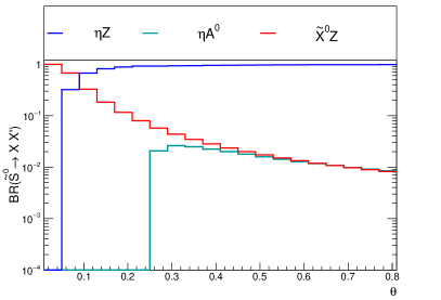
Figure 9: Branching ratios (BR) of $\tilde{S}^{0}$ for $M_{A}=3$ TeV, $M_{V}=3.5$ TeV and $\widetilde{g}=3$. On the left as a function of $\theta$ with $r=0.6$ and on the right as a function of $r$ with $\theta=0.2$. The behaviour of the charged $\tilde{S}^{\pm}$ is analogous, replacing $Z$ by $W^{\pm}$ and $A^{0}$ by $A^{\pm}$.

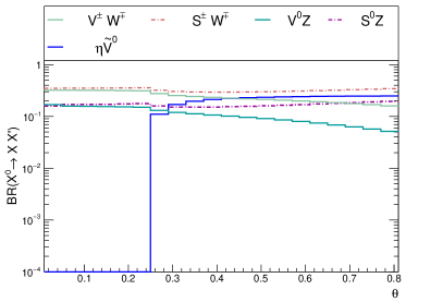
Figure 10: Left: ratios (BR) of $\tilde{V}^{0}$ for $M_{A}=3$ TeV, $M_{V}=3.5$ TeV. It is independent of $\widetilde{g}$ and $r$. This state decays only to $h\tilde{X}^{0}$ and $\eta X^{0}$. Right:Branching ratios (BR) of $X^{0}$ for $M_{A}=3$ TeV and $M_{V}=2.5$ TeV. It is independent of $\widetilde{g}$ and $r$.

The branching ratio of $\tilde{X}^{0}$ is independent on $\tilde{g}$, $r$ and $\theta$, and this state will decay into $h\tilde{V}^{0}$, $Z\tilde{S}^{0}$, $W^{\pm}\tilde{S}^{\mp}$ in the ratio of $(1:1:2)$.

References

- (1) A. P. Balachandran, A. Stern and C. G. Trahern, Non Linear Models as Gauge Theories, Phys. Rev. D19 (1979) 2416.
- (2) E. Eichten and K. D. Lane, Dynamical Breaking of Weak Interaction Symmetries, Phys. Lett. B90 (1980) 125–130.
- (3) S. Weinberg, Implications of Dynamical Symmetry Breaking, Phys. Rev. D13 (1976) 974–996.
- (4) L. Susskind, Dynamics of Spontaneous Symmetry Breaking in the Weinberg-Salam Theory, Phys. Rev. D20 (1979) 2619–2625.
- (5) E. Farhi and L. Susskind, Technicolor, Phys. Rept. 74 (1981) 277.
- (6) S. Dimopoulos and L. Susskind, Mass Without Scalars, Nucl. Phys. B155 (1979) 237–252.
- (7) S. K. Dimopoulos and J. R. Ellis, Challenges for extended technicolour theories, Nucl. Phys. B 182 (Sep, 1980) 505–528. 31 p.
- (8) M. E. Peskin and T. Takeuchi, A New constraint on a strongly interacting Higgs sector, Phys. Rev. Lett. 65 (1990) 964–967.
- (9) D. B. Kaplan and H. Georgi, SU(2) x U(1) Breaking by Vacuum Misalignment, Phys. Lett. B136 (1984) 183.
- (10) H. Georgi and D. B. Kaplan, Composite Higgs and Custodial SU(2), Phys. Lett. B145 (1984) 216.
- (11) M. J. Dugan, H. Georgi and D. B. Kaplan, Anatomy of a Composite Higgs Model, Nucl. Phys. B254 (1985) 299.
- (12) B. Bellazzini, C. Csáki and J. Serra, Composite Higgses, Eur. Phys. J. C74 (2014) 2766, [1401.2457].
- (13) G. Panico and A. Wulzer, The Composite Nambu-Goldstone Higgs, Lect. Notes Phys. 913 (2016) pp.1–316, [1506.01961].
- (14) K. Agashe, R. Contino and A. Pomarol, The Minimal composite Higgs model, Nucl. Phys. B719 (2005) 165–187, [hep-ph/0412089].
- (15) G. F. Giudice, C. Grojean, A. Pomarol and R. Rattazzi, The Strongly-Interacting Light Higgs, JHEP 06 (2007) 045, [hep-ph/0703164].
- (16) R. Contino, M. Ghezzi, C. Grojean, M. Muhlleitner and M. Spira, Effective Lagrangian for a light Higgs-like scalar, JHEP 07 (2013) 035, [1303.3876].
- (17) G. Buchalla, O. Cata and C. Krause, A Systematic Approach to the SILH Lagrangian, Nucl. Phys. B894 (2015) 602–620, [1412.6356].
- (18) D. B. Kaplan, Flavor at SSC energies: A New mechanism for dynamically generated fermion masses, Nucl. Phys. B365 (1991) 259–278.
- (19) R. Contino and G. Servant, Discovering the top partners at the LHC using same-sign dilepton final states, JHEP 06 (2008) 026, [0801.1679].
- (20) G. Dissertori, E. Furlan, F. Moortgat and P. Nef, Discovery potential of top-partners in a realistic composite Higgs model with early LHC data, JHEP 09 (2010) 019, [1005.4414].
- (21) J. Li, D. Liu and J. Shu, Towards the fate of natural composite Higgs model through single search at the 8 TeV LHC, JHEP 11 (2013) 047, [1306.5841].
- (22) T. Flacke, J. H. Kim, S. J. Lee and S. H. Lim, Constraints on composite quark partners from Higgs searches, JHEP 05 (2014) 123, [1312.5316].
- (23) O. Matsedonskyi, G. Panico and A. Wulzer, On the Interpretation of Top Partners Searches, JHEP 12 (2014) 097, [1409.0100].
- (24) G. Cacciapaglia, H. Cai, T. Flacke, S. J. Lee, A. Parolini and H. Serôdio, Anarchic Yukawas and top partial compositeness: the flavour of a successful marriage, JHEP 06 (2015) 085, [1501.03818].
- (25) J. Serra, Beyond the Minimal Top Partner Decay, JHEP 09 (2015) 176, [1506.05110].
- (26) M. Backovic, T. Flacke, J. H. Kim and S. J. Lee, Search Strategies for TeV Scale Fermionic Top Partners with Charge 2/3, JHEP 04 (2016) 014, [1507.06568].
- (27) O. Matsedonskyi, G. Panico and A. Wulzer, Top Partners Searches and Composite Higgs Models, JHEP 04 (2016) 003, [1512.04356].
- (28) M. Buchkremer, G. Cacciapaglia, A. Deandrea and L. Panizzi, Model Independent Framework for Searches of Top Partners, Nucl. Phys. B876 (2013) 376–417, [1305.4172].
- (29) D. Barducci, A. Belyaev, M. Buchkremer, G. Cacciapaglia, A. Deandrea, S. De Curtis et al., Framework for Model Independent Analyses of Multiple Extra Quark Scenarios, JHEP 12 (2014) 080, [1405.0737].
- (30) R. Contino, D. Marzocca, D. Pappadopulo and R. Rattazzi, On the effect of resonances in composite Higgs phenomenology, JHEP 10 (2011) 081, [1109.1570].
- (31) M. Low, A. Tesi and L.-T. Wang, Composite spin-1 resonances at the LHC, Phys. Rev. D92 (2015) 085019, [1507.07557].
- (32) C. Niehoff, P. Stangl and D. M. Straub, Direct and indirect signals of natural composite Higgs models, JHEP 01 (2016) 119, [1508.00569].
- (33) G. Cacciapaglia, H. Cai, A. Deandrea, T. Flacke, S. J. Lee and A. Parolini, Composite scalars at the LHC: the Higgs, the Sextet and the Octet, JHEP 11 (2015) 201, [1507.02283].
- (34) G. Ferretti, Gauge theories of Partial Compositeness: Scenarios for Run-II of the LHC, 1604.06467.
- (35) E. Katz, A. E. Nelson and D. G. E. Walker, The Intermediate Higgs, JHEP 08 (2005) 074, [hep-ph/0504252].
- (36) J. Mrazek, A. Pomarol, R. Rattazzi, M. Redi, J. Serra and A. Wulzer, The Other Natural Two Higgs Doublet Model, Nucl. Phys. B853 (2011) 1–48, [1105.5403].
- (37) E. Bertuzzo, T. S. Ray, H. de Sandes and C. A. Savoy, On Composite Two Higgs Doublet Models, JHEP 05 (2013) 153, [1206.2623].
- (38) M. Frigerio, A. Pomarol, F. Riva and A. Urbano, Composite Scalar Dark Matter, JHEP 07 (2012) 015, [1204.2808].
- (39) D. Marzocca and A. Urbano, Composite Dark Matter and LHC Interplay, JHEP 07 (2014) 107, [1404.7419].
- (40) T. A. Ryttov and F. Sannino, Ultra Minimal Technicolor and its Dark Matter TIMP, Phys. Rev. D78 (2008) 115010, [0809.0713].
- (41) J. Galloway, J. A. Evans, M. A. Luty and R. A. Tacchi, Minimal Conformal Technicolor and Precision Electroweak Tests, JHEP 10 (2010) 086, [1001.1361].
- (42) G. Cacciapaglia and F. Sannino, Fundamental Composite (Goldstone) Higgs Dynamics, JHEP 1404 (2014) 111, [1402.0233].
- (43) Y. Hochberg, E. Kuflik, H. Murayama, T. Volansky and J. G. Wacker, Model for Thermal Relic Dark Matter of Strongly Interacting Massive Particles, Phys. Rev. Lett. 115 (2015) 021301, [1411.3727].
- (44) M. Hansen, K. Langaeble and F. Sannino, SIMP model at NNLO in chiral perturbation theory, Phys. Rev. D92 (2015) 075036, [1507.01590].
- (45) T. Appelquist, P. S. Rodrigues da Silva and F. Sannino, Enhanced global symmetries and the chiral phase transition, Phys. Rev. D60 (1999) 116007, [hep-ph/9906555].
- (46) Z.-y. Duan, P. S. Rodrigues da Silva and F. Sannino, Enhanced global symmetry constraints on epsilon terms, Nucl. Phys. B592 (2001) 371–390, [hep-ph/0001303].
- (47) S. R. Coleman, J. Wess and B. Zumino, Structure of phenomenological Lagrangians. 1., Phys. Rev. 177 (1969) 2239–2247.
- (48) C. G. Callan, Jr., S. R. Coleman, J. Wess and B. Zumino, Structure of phenomenological Lagrangians. 2., Phys. Rev. 177 (1969) 2247–2250.
- (49) M. Bando, T. Kugo and K. Yamawaki, Nonlinear Realization and Hidden Local Symmetries, Phys. Rept. 164 (1988) 217–314.
- (50) P. Batra and Z. Chacko, Symmetry Breaking Patterns for the Little Higgs from Strong Dynamics, Phys. Rev. D77 (2008) 055015, [0710.0333].
- (51) A. Hietanen, R. Lewis, C. Pica and F. Sannino, Fundamental Composite Higgs Dynamics on the Lattice: SU(2) with Two Flavors, JHEP 07 (2014) 116, [1404.2794].
- (52) V. Drach, A. Hietanen, C. Pica, J. Rantaharju and F. Sannino, Template Composite Dark Matter : SU(2) gauge theory with 2 fundamental flavours, in Proceedings, 33rd International Symposium on Lattice Field Theory (Lattice 2015), 2015. 1511.04370.
- (53) B. Gripaios, A. Pomarol, F. Riva and J. Serra, Beyond the Minimal Composite Higgs Model, JHEP 04 (2009) 070, [0902.1483].
- (54) A. Arbey, G. Cacciapaglia, H. Cai, A. Deandrea, S. Le Corre and F. Sannino, Fundamental Composite Electroweak Dynamics: Status at the LHC, 1502.04718.
- (55) G. ’t Hooft, Naturalness, chiral symmetry, and spontaneous chiral symmetry breaking, NATO Sci. Ser. B 59 (1980) 135.
- (56) G. Cacciapaglia and F. Sannino, An Ultraviolet Chiral Theory of the Top for the Fundamental Composite (Goldstone) Higgs, Phys. Lett. B755 (2016) 328–331, [1508.00016].
- (57) R. S. Chivukula, E. H. Simmons, H.-J. He, M. Kurachi and M. Tanabashi, Deconstructed Higgsless models with one-site delocalization, Phys. Rev. D71 (2005) 115001, [hep-ph/0502162].
- (58) G. Ferretti and D. Karateev, Fermionic UV completions of Composite Higgs models, JHEP 03 (2014) 077, [1312.5330].
- (59) J. Barnard, T. Gherghetta and T. S. Ray, UV descriptions of composite Higgs models without elementary scalars, JHEP 02 (2014) 002, [1311.6562].
- (60) O. Matsedonskyi, G. Panico and A. Wulzer, Light Top Partners for a Light Composite Higgs, JHEP 01 (2013) 164, [1204.6333].
- (61) R. Rattazzi, V. S. Rychkov, E. Tonni and A. Vichi, Bounding scalar operator dimensions in 4D CFT, JHEP 12 (2008) 031, [0807.0004].
- (62) V. S. Rychkov and A. Vichi, Universal Constraints on Conformal Operator Dimensions, Phys. Rev. D80 (2009) 045006, [0905.2211].
- (63) R. Rattazzi, S. Rychkov and A. Vichi, Bounds in 4D Conformal Field Theories with Global Symmetry, J. Phys. A44 (2011) 035402, [1009.5985].
- (64) C. Pica and F. Sannino, Anomalous Dimensions of Conformal Baryons, Phys. Rev. D94 (2016) 071702, [1604.02572].
- (65) L. Vecchi, The anomalous dimension of spin-1/2 baryons in many flavors QCD, 1607.02740.
- (66) R. Casalbuoni, S. De Curtis, D. Dominici, F. Feruglio and R. Gatto, Constraints on the Bess model from precision electroweak data. Specialization to technicolor and extended technicolor, Phys. Lett. B269 (1991) 361–370.
- (67) R. Casalbuoni, S. De Curtis, A. Deandrea, N. Di Bartolomeo, R. Gatto, D. Dominici et al., The Extended BESS model: Bounds from precision electroweak measurements, Nucl. Phys. B409 (1993) 257–289, [hep-ph/9209290].
- (68) R. Casalbuoni, A. Deandrea, S. De Curtis, D. Dominici, R. Gatto and M. Grazzini, Degenerate BESS model: The Possibility of a low-energy strong electroweak sector, Phys. Rev. D53 (1996) 5201–5221, [hep-ph/9510431].
- (69) R. Casalbuoni, S. De Curtis, D. Dominici, F. Feruglio and R. Gatto, Vector and Axial Vector Bound States From a Strongly Interacting Electroweak Sector, Int. J. Mod. Phys. A4 (1989) 1065.
- (70) D. Marzocca, M. Serone and J. Shu, General Composite Higgs Models, JHEP 08 (2012) 013, [1205.0770].
- (71) J. Wess and B. Zumino, Consequences of anomalous Ward identities, Phys. Lett. B37 (1971) 95–97.
- (72) E. Witten, Current Algebra Theorems for the U(1) Goldstone Boson, Nucl. Phys. B156 (1979) 269–283.
- (73) A. Belyaev, R. Foadi, M. T. Frandsen, M. Jarvinen, F. Sannino and A. Pukhov, Technicolor Walks at the LHC, Phys. Rev. D79 (2009) 035006, [0809.0793].
- (74) B. Bellazzini, C. Csaki, J. Hubisz, J. Serra and J. Terning, Composite Higgs Sketch, JHEP 11 (2012) 003, [1205.4032].
- (75) O. Castillo-Felisola, C. Corral, M. González, G. Moreno, N. A. Neill, F. Rojas et al., Higgs Boson Phenomenology in a Simple Model with Vector Resonances, Eur. Phys. J. C73 (2013) 2669, [1308.1825].
- (76) M. Spira, A. Djouadi, D. Graudenz and P. M. Zerwas, Higgs boson production at the LHC, Nucl. Phys. B453 (1995) 17–82, [hep-ph/9504378].
- (77) H. Cai, Higgs-Z-photon Coupling from Effect of Composite Resonances, JHEP 04 (2014) 052, [1306.3922].
- (78) ATLAS collaboration, G. Aad et al., Constraints on new phenomena via Higgs boson couplings and invisible decays with the ATLAS detector, JHEP 11 (2015) 206, [1509.00672].
- (79) The ALEPH, DELPHI, L3, OPAL Collaborations, the LEP Electroweak Working Group, Electroweak Measurements in Electron-Positron Collisions at W-Boson-Pair Energies at LEP, Phys. Rept. 532 (2013) 119, [1302.3415].
- (80) M. E. Peskin and T. Takeuchi, Estimation of oblique electroweak corrections, Phys. Rev. D46 (1992) 381–409.
- (81) R. Barbieri, A. Pomarol, R. Rattazzi and A. Strumia, Electroweak symmetry breaking after LEP-1 and LEP-2, Nucl. Phys. B703 (2004) 127–146, [hep-ph/0405040].
- (82) R. Foadi, M. T. Frandsen, T. A. Ryttov and F. Sannino, Minimal Walking Technicolor: Set Up for Collider Physics, Phys. Rev. D76 (2007) 055005, [0706.1696].
- (83) D. Becciolini, D. B. Franzosi, R. Foadi, M. T. Frandsen, T. Hapola and F. Sannino, Custodial Vector Model, Phys. Rev. D92 (2015) 015013, [1410.6492].
- (84) R. Contino and M. Salvarezza, One-loop effects from spin-1 resonances in Composite Higgs models, JHEP 07 (2015) 065, [1504.02750].
- (85) D. Ghosh, M. Salvarezza and F. Senia, Extending the Analysis of Electroweak Precision Constraints in Composite Higgs Models, 1511.08235.
- (86) A. Pich, I. Rosell and J. J. Sanz-Cillero, Oblique S and T Constraints on Electroweak Strongly-Coupled Models with a Light Higgs, JHEP 01 (2014) 157, [1310.3121].
- (87) R. Contino and M. Salvarezza, Dispersion Relations for Electroweak Observables in Composite Higgs Models, Phys. Rev. D92 (2015) 115010, [1511.00592].
- (88) Particle Data Group collaboration, K. A. Olive et al., Review of Particle Physics, Chin. Phys. C38 (2014) 090001.
- (89) J. Alwall, R. Frederix, S. Frixione, V. Hirschi, F. Maltoni, O. Mattelaer et al., The automated computation of tree-level and next-to-leading order differential cross sections, and their matching to parton shower simulations, JHEP 07 (2014) 079, [1405.0301].
- (90) A. Alloul, N. D. Christensen, C. Degrande, C. Duhr and B. Fuks, FeynRules 2.0 - A complete toolbox for tree-level phenomenology, Comput.Phys.Commun. 185 (2014) 2250–2300, [1310.1921].
- (91) C. Degrande, C. Duhr, B. Fuks, D. Grellscheid, O. Mattelaer et al., UFO - The Universal FeynRules Output, Comput.Phys.Commun. 183 (2012) 1201–1214, [1108.2040].
- (92) R. D. Ball et al., Parton distributions with LHC data, Nucl. Phys. B867 (2013) 244–289, [1207.1303].
- (93) G. Cacciapaglia, A. Deandrea and S. De Curtis, Nearby resonances beyond the Breit-Wigner approximation, Phys. Lett. B682 (2009) 43–49, [0906.3417].
- (94) J. de Blas, J. M. Lizana and M. Perez-Victoria, Combining searches of Z’ and W’ bosons, JHEP 01 (2013) 166, [1211.2229].
- (95) D. Buarque Franzosi and R. Foadi, Probing Near-Conformal Technicolor through Weak Boson Scattering, Phys. Rev. D88 (2013) 015013, [1209.5913].
- (96) K. Mohan and N. Vignaroli, Vector resonances in weak-boson-fusion at future pp colliders, JHEP 10 (2015) 031, [1507.03940].
- (97) Search for new phenomena in the dilepton final state using proton-proton collisions at = 13 TeV with the ATLAS detector, Tech. Rep. ATLAS-CONF-2015-070, CERN, Dec, 2015.
- (98) Search for diboson resonances in the final state in collisions at TeV with the ATLAS detector, Tech. Rep. ATLAS-CONF-2015-068, CERN, Dec, 2015.
- (99) CMS collaboration, C. Collaboration, Search for a Narrow Resonance Produced in 13 TeV pp Collisions Decaying to Electron Pair or Muon Pair Final States, Tech. Rep. CMS-PAS-EXO-15-005, 2015.
- (100) CMS collaboration, C. Collaboration, Search for massive resonances decaying into pairs of boosted W and Z bosons at = 13 TeV, Tech. Rep. CMS-PAS-EXO-15-002, 2015.
- (101) R. Arthur, V. Drach, M. Hansen, A. Hietanen, C. Pica and F. Sannino, SU(2) Gauge Theory with Two Fundamental Flavours: a Minimal Template for Model Building, 1602.06559.
- (102) T. Han, J. Sayre and S. Westhoff, Top-Quark Initiated Processes at High-Energy Hadron Colliders, JHEP 04 (2015) 145, [1411.2588].
- (103) M. S. Chanowitz and M. K. Gaillard, The TeV Physics of Strongly Interacting W’s and Z’s, Nucl. Phys. B261 (1985) 379–431.
- (104) E. Bothmann, P. Ferrarese, F. Krauss, S. Kuttimalai, S. Schumann and J. Thompson, Aspects of pQCD at a 100 TeV future hadron collider, 1605.00617.
- (105) B. Richter, High Energy Colliding Beams; What Is Their Future?, Rev. Accel. Sci. Tech. 7 (2014) 1–8, [1409.1196].
- (106) T. G. Rizzo, Mass Reach Scaling for Future Hadron Colliders, Eur. Phys. J. C75 (2015) 161, [1501.05583].