Consequences of tidal interaction between disks and orbiting protoplanets for the evolution of multi-planet systems with architecture resembling that of Kepler 444

Abstract

We study orbital evolution of multi-planet systems with masses in the terrestrial planet regime induced through tidal interaction with a protoplanetary disk assuming that this is the dominant mechanism for producing orbital migration and circularization. We develop a simple analytic model for a system that maintains consecutive pairs in resonance while undergoing orbital circularization and migration. This model enables migration times for each planet to be estimated once planet masses, circularization times and the migration time for the innermost planet are specified. We applied it to a system with the current architecture of Kepler 444 adopting a simple protoplanetary disk model and planet masses that yield migration times inversely proportional to the planet mass, as expected if they result from torques due to tidal interaction with the protoplanetary disk. Furthermore the evolution time for the system as a whole is comparable to current protoplanetary disk lifetimes.

In addition we have performed a number of numerical simulations with input data obtained from this model. These indicate that although the analytic model is inexact, relatively small corrections to the estimated migration rates yield systems for which period ratios vary by a minimal extent.

Because of relatively large deviations from exact resonance in the observed system of up to $2\%,$ the migration times obtained in this way indicate only weak convergent migration such that a system for which the planets did not interact would contract by only $\sim 1\%$ although undergoing significant inward migration as a whole. We have also performed additional simulations to investigate conditions under which the system could undergo significant convergent migration before reaching its final state. These indicate that migration times have to be significantly shorter and resonances between planet pairs significantly closer during such an evolutionary phase. Relative migration rates would then have to decrease allowing period ratios to increase to become more distant from resonances as the system approached its final state in the inner regions of the protoplanetary disk.

Planet formation-Planetary systems-Resonances -Tidal interactions

1 Introduction

The Kepler mission has discovered an abundance of confirmed and candidate planets orbiting close to their host stars ( Batalha et al. 2013). Many of these are in highly compact planetary systems. A significant number contain pairs that are close to first order commensurabilities. Lissauer et al. (2011)a found Kepler candidates in short period orbits in multi-resonant configurations. For example the Kepler 223 system contains four planets exhibiting the mean motion ratios 8:6:4:3 and Kepler 80 is a near-resonant system of five planets in which there are two three body mean motion resonances $2n_{2}-5n_{3}+3n_{4}\sim 0$ and $2n_{3}-6n_{4}+4n_{5}\sim 0,$ with $n_{i}$ being the mean motion of planet $i.$ In addition the Kepler 60 system has three planets with the inner pair very close to a 5:4 commensurability and the outer pair very close to a 4:3 commensurability (Steffen et al. 2013) .

The recently confirmed Kepler 444 system contains five transiting, sub-Earths (Campante et al. 2015). This system is highly compact with all planets orbiting the parent star within 0.08 AU. In addition the orbits are consistent with near-coplanarity. Consecutive planet pairs are close to first order orbital commensurabilities, with relative deviations of less than $2\%$ in excess of 5:4, 4:3, 5:4, and 5:4 resonances. The central star is metal poor. It and hence the planetary system has an age of 11:2 G y., making it the oldest known system of terrestrial planets. Furthermore it has a binary companion at a projected separation of $\sim$ 60 AU (Campante et al. 2015). If this was that close when the protoplanetary disk was present, it is likely to have influenced planet formation and evolution. These features make it of special interest in the context of planet formation theories.

Tightly packed resonant planetary systems of this kind are of interest on account of what their dynamics can tell us about their formation and early orbital evolution. The formation of resonant chains in tightly packed systems of planets is expected to occur as a result of convergent orbital migration produced by the action of torques resulting from tidal interaction with the protoplanetary disk from which they formed (eg. Cresswell & Nelson 2006; Terquem and Papaloizou 2007).

Migration due to tidal interaction with the disk has also been suggested as a mechanism through which planets end up on short period orbits in order to avoid problems associated with in situ formation ( e.g. Raymond et al. 2008). However, the total amount of radial migration does not need to be large in order to form near commensurabilities, and as illustrated in this paper, it is not necessary to assume that the planets formed beyond an ice line and then underwent very large changes to their semi-major axes.

In this paper we study the evolution of multi-planet systems with masses that are small enough that the tidal interaction with the disk, with the exception of the estimation of coorbital torques that can be important for migration and which are nearly always nonlinear (Paardekooper & Papaloizou 2009), is in the linear regime.

We develop a simplified general analytic model describing the evolution of a system of $N$ coplanar resonantly coupled planets in near circular orbits with fixed orbital period ratios. This enables rates of convergent migration to be estimated given an orbital architecture, circularization times estimated from the theory of disk-planet tidal interaction, and the planet masses. This is applied to a system with the current architecture of the Kepler 444 system. As radii are known but masses unknown for the planets in that system, we work with a system which has the same architecture but masses determined such that estimated planetary migration rates are approximately inversely proportional to their masses, as is expected for disk-planet tidal interactions under gravity.

We perform numerical simulations to study the evolution of planetary systems of the type described above, as well as systems with larger masses and systems with consecutive pairs closer to resonance. The analytic model is used as a guide and to provide input parameters. The simulations are carried out to investigate the maintenance and formation of comensurabilities as the system migrates inwards significantly, changing its radial scale on a time scale characteristic of the lifetime of current protoplanetary disks. We find that significant convergent migration does not occur with migration rates estimated assuming a system with a steady architecture corresponding to that of Kepler 444. In order for this to occur, consecutive pairs in the system need to have been closer to resonance during an early phase when relative migration rates were faster. We speculate that these rates could have slowed as the system approached the inner edge of a truncated protoplanetary disk.

The plan of the paper is as follows. In Section 2 we review relevant aspects of the theory of orbital migration induced by the tidal interaction of protoplanets with protoplanetary disks, going on to give estimates of the orbital circularization times arising from both tidal interaction with the disk and the central star in Sections 2.1 and 2.2. In Section 3 we set out the basic equations for a model of a planetary system interacting with a protoplanetary disk in which it is treated as $N$ interacting bodies.

We then go on to formulate the analytic model for a planetary system with consecutive pairs in resonance undergoing orbital migration and circularization in Section 4. In this formalism gravitational interaction only occurs between neighbouring planets through either one or two retained resonant angles. However, it is assumed that three body resonances of the Laplace type are absent. The procedure may be applied to a system as a whole or to two or more uncoupled subsystems. For a system or subsystem, with given masses, in which commensurabilities are maintained, the model leads to relationships between migration and circularization times that are developed in Section 4.4. These enable migration times for each planet to be determined once planet masses, circularization times and the migration time for one of them is specified. Migration times estimated in this way were used as input data for the detailed numerical simulations.

Specification of the input orbital parameters and planet masses for the simulations is described in detail in Sections 5-5.2.2. How results may be scaled so that the initial systems start at an expanded length scale and finish in configuration resembling the initial one is indicated in Section 5.3. We go on to describe the results of the simulations in Sections 6 - 6.3.3 and then summarize and discuss our results in Section 7.

2 Orbital migration and circularization due to tidal interaction with the protoplanetary disk

It is well known that orbiting protoplanets embedded in a protoplanetary disk experience orbital migration and circularization as a result of tidal interaction with it. (see eg. Ward 1997; Papaloizou & Terquem 2006; Correa-Otto et al. 2013, Baruteau et al. 2014). While the orbital circularization of low mass protoplanets may be robustly estimated from a linear response calculation (see Section 2.1 below) the situation regarding orbital migration is less clear largely because of significant contributions from nonlinear coorbital torques that depend on conditions close to the planet as well as details of the protoplanetary disk model (e.g., Paardekooper & Mellema 2006, Paardekooper & Papaloizou 2009 ). It is well known that simple models of locally isothermal disks with surface density profiles that render coorbital torques ineffective produce inward migration times for low mass protoplanets that are too small by between one and two orders of magnitude (eg. Ida & Lin 2008).

Various mechanisms for reducing or reversing such migration have been proposed. These include the introduction of stochastic torques resulting from turbulence (Nelson & Papaloizou 2004), invoking an eccentric disk (eg. Papaloizou 2002), the operation of coorbital torques induced by entropy gradients (eg. Paardekooper & Mellema 2006). the influence of outwardly propagating density waves (eg. Podlewska-Gaca et al. 2012), the effects of a magnetic field ( Terquem 2003, Guilet et al. 2013), the influence of a turbulence driven wind on the disk surface density profile ( Suzuki et al. 2010, Ogihara et al. 2015 ), and more recently the effects of heat radiation from an embedded protoplanet on an asymmetric disk mass distribution (Benitez-Llambay et al. 2015 ). Some or all of these mechanisms may play a role in different regions of the protoplanetary disk making the determination of migration rates problematic.

In the work presented here we shall instead consider the estimation of migration rates from the orbital configuration of a near resonant system together with circularization times estimated from disk planet interaction, assuming that these can be related. In general as was found by Ida & Lin (2008) for population synthesis modelling, theoretical migration rates determined for locally isothermal disk models need to be significantly reduced to match these estimates. We suppose that one or more of the mechanisms enumerated above act to provide the required reduction in the inner parts of the protoplanetary disk that we consider, However, for the low mass planets we consider, we shall retain the expected approximate proportionality of the migration time to the reciprocal of the planet mass, as this is expected on very general grounds for purely gravitational interaction ( eg. Papaloizou & Terquem 2006; Baruteau et al. 2014). But note that this could be departed from if effects due to heat radiation are very significant as proposed by Benitez-Llambay et al. (2015 ). Note that the circularization times discussed below are inversely proportional to the planet mass.

2.1 Estimation of the orbital circularization time

The circularization time obtained from a linear response calculation of the disk-protoplanet interaction for a protoplanet of mass $m_{j}$ with small eccentricity is given by (see Tanaka & Ward 2004)

$$t_{e,j}=1.3\times 10^{3}\frac{M}{M_{\odot}}\frac{M}{m_{j}}\frac{\pi}{n_{j}}\left(\frac{H}{a_{j}}\right)^{4}\frac{M_{J}}{\pi\Sigma_{p}a_{j}^{2}}$$ (1)

Here the semi-major axis of the planet is $a_{j}$ and its mean motion $n_{j}.$ The local disk semi-thickness is $H,$ the surface density at the position of the planet is $\Sigma_{p},$ the central mass is $M$ and $M_{J}$ is a Jovian mass. The disk is assumed to be locally isothermal. In order to estimate $H$ we adopt the simple estimate given by

$$\frac{H}{a_{j}}=\sqrt{\frac{{\cal R}T_{j}}{\mu n_{j}^{2}a_{j}^{2}}}$$ (2)

where the disk temperature at the location of the planet is $T_{j}=T_{eff}\sqrt{R_{*}/2a_{j}}.$ Here the mean molecular weight is $\mu,$ $T_{eff}$ is the effective temperature of the central star, $R_{*}$ is its radius and ${\cal R}$ is the gas constant. As an ilustration we adopt the stellar parameters to be those for Kepler 444 (Campante et al. 2015), and $\mu=2.$ Then we obtain

$$\frac{H}{a_{j}}=0.02\left(\frac{a_{j}}{0.1AU}\right)^{1/4}.$$ (3)

For aspect ratios of the above estimated magnitude and the planet masses we consider, the disk planet interaction is expected to be in the linear type I migration regime (eg. Ward 1997), justifying the use of equation (1), from which we obtain

$$t_{e,j}=1.6\times 10^{-4}\frac{M}{m_{j}}\frac{\pi}{n_{j}}\frac{a_{j}}{0.1AU}\frac{M_{J}}{\pi\Sigma_{p}a_{j}^{2}}.$$ (4)

We note that for the special case with $\Sigma_{p}\propto a_{j}^{-1},$ $t_{c}\propto n_{j}^{-1}$ scales as the orbital period. Then we have

$$t_{e,j}=3.2\times 10^{-4}\frac{M}{m_{j}}\frac{\pi}{n_{j}}\left(\frac{a_{j}}{0.1AU}\frac{M_{J}}{M_{D}(a_{j})}\right).$$ (5)

In the above expression $M_{D}(a_{j})$ is the disk mass interior to $a_{j}$ and the quantity in brackets is constant. Thus for $M_{D}=M_{J}$ interior to $1AU,$ we obtain $t_{c}\sim 360$ orbital periods for a one earth mass protoplanet and $M=0.758M_{\oplus}.$ We note that if the above mass scaling applies out to $5AU,$ the interior disk mass would correspond to two and a half times that of the minimum mass solar nebula. However, we stress that we are only concerned with the dynamics interior to $1AU$ and this would be unaffected if the disk surface density was decreased at larger radii so that such an extrapolation does not apply.

2.2 Orbital circularization due to tides from the central star

The circularization timescale due to tidal interaction with the star was obtained from Goldreich & Soter (1966) in the form

$$t_{e,j}^{s}=\frac{0.69\rho_{pj}^{5/3}a_{j}^{13/2}Q^{\prime}}{G^{1/2}M^{3/2}m_{j}^{2/3}}$$ (6)

where $R_{pj}$ is the radius of planet $j$ and $\rho_{pj}$ is its mean density. The quantity $Q^{\prime}=3Q/(2k_{2}),$ where $Q$ is the tidal dissipation function and $k_{2}$ is the Love number. The values of these tidal parameters applicable to exoplanets are very uncertain. However, for solar system planets in the terrestrial mass range, Goldreich & Soter (1966) give estimates for $Q$ in the range 10–500 and $k_{2}\sim 0.3$, which correspond to $Q^{\prime}$ in the range 50–2500. We may also write (6) in the form

$$t_{e,j}^{s}=\frac{9.6\times 10^{5}(\rho_{pj}/(1gmcm^{-3}))^{5/3}(a_{j}/0.04AU)^{13/2}(Q^{\prime}/100)}{(m_{j}/M_{\oplus})^{2/3}(M/M_{\oplus})^{3/2}}y.$$ (7)

From this we see that sub earth mass rocky planets orbiting further out than $0.04AU$ such as those in Kepler 444 are unlikely to more than barely circularize due to this mechanism within an expected formation time of $10^{6-7}y.$ It is accordingly far less effective than interaction with the disk during this period so we shall neglect it. However, it may result in a small rate of separation of the system away from resonance after disk dispersal (eg. Papaloizou 2011).

We note that convergent disk migration of consecutive pairs of planets leads naturally to multiple systems in resonant chains of the type considered here (eg. Cresswell & Nelson 2006; Papaloizou & Terquem 2010; Baruteau et al. 2014). Note that if they start out close to resonance, these configurations may be produced with the system as a whole undergoing little net radial migration.

3 Basic equations for an N body model of a planetary system interacting with a disk

We begin by considering a system of $N$ planets and a central star interacting gravitationally. The equations of motion are:

$${d^{2}{\bf r}_{j}\over dt^{2}}=-{GM{\bf r}_{j}\over|{\bf r}_{j}|^{3}}-\sum_{k=1\neq j}^{N}{Gm_{k}\left({\bf r}_{j}-{\bf r}_{k}\right)\over|{\bf r}_{j}-{\bf r}_{k}|^{3}}-{\bf\Gamma}-{\bf\Gamma}_{j}-{\bf B}_{j}\;,$$ (8)

where $M$, $m_{j},$ and ${\bf r}_{j}$ denote the mass of the central star, the mass of planet $j,$ and the position vector of planet $j,$ respectively. The acceleration of the coordinate system based on the central star (indirect term) is:

$${\bf\Gamma}=\sum_{j=1}^{N}{Gm_{j}{\bf r}_{j}\over|{\bf r}_{j}|^{3}},$$ (9)

Orbital circularization due to tidal interaction with the disk is dealt with through the addition of a frictional damping force taking the form (see eg. Papaloizou & Terquem 2010)

$${\bf\Gamma}_{j}=-\frac{2}{|{\bf r}_{j}|^{2}t_{e,j}}\left(\frac{d{\bf r}_{j}}{dt}\cdot{\bf r}_{j}\right){\bf r}_{j}$$ (10)

Migration torques are included through ${\bf B}_{j}$ which takes the form ( see eg. Terquem & Papaloizou 2007)

$${\bf B}_{j}=-\frac{{\bf r}_{j}\times\left({\bf r}_{j}\times(d{\bf r}_{j}/dt)\right)}{3t_{mig,j}|{\bf r}_{j}|^{2}},$$ (11)

where $t_{mig,j}$ is defined to be the migration time for planet $j,$ being the characteristic time on which the mean motion increases. Note that the characteristic time on which the specific angular momentum decreases is $3t_{mig,j}.$ Hence the factor of 3 in the denominator of equation (11).

4 Analytic model for a planetary system with consecutive pairs in resonance undergoing orbital migration and circularization

We develop an analytic model that shows how a system of $N$ planets undergoes orbital evolution driven by orbital migration and circularization driven by tidal interaction with a protoplanetary disk. The coupling between the planets occurs through the behaviour of resonant angles, which may librate, so producing evolution of orbital elements after time averaging. However, significant deviations from exact commensurability may occur. We begin by formulating equations governing the system without forces associated with disk planet interaction. In that case a Hamiltonian formalism can be used. We then go on to add effects arising from interaction with the disk. The starting point is the same as in Papaloizou (2015). However, in contrast to the work there, the discussion here includes the effects of orbital migration and considers a system with an arbitrary number of planets.

4.1 Coordinate system

We adopt Jacobi coordinates (eg. Sinclair 1975 ) for which the radius vector of planet $j,$ ${\bf r}_{j},$ is measured relative to the centre of mass of the system comprised of $M$ and all other planets interior to $j,$ for $j=1,2,3,...,N.$ Here $j=1$ corresponds to the innermost planet and $j=N$ to the outermost planet.

4.2 Hamiltonian for the system without disk interaction

The Hamiltonian for the system governed by (8) with orbital migration and circularization absent can be written, correct to second order in the planetary masses, in the form:

$$H = \sum_{j=1}^{N}\left({1\over 2}m_{j}|\dot{\bf r}_{j}|^{2}-{GM_{j}m_{j}\over|{\bf r}_{j}|}\right)$$ (12)

$$- \sum_{j=1}^{N}\sum_{k=j+1}^{N}Gm_{j}m_{k}\left({1\over|{\bf r}_{jk}|}-{{\bf r}_{j}\cdot{\bf r}_{k}\over|{\bf r}_{k}|^{3}}\right).$$

Here $M_{j}=M+m_{j}$ and ${\bf r}_{jk}={\bf r}_{j}-{\bf r}_{k}.$

Assuming, the planetary system is strictly coplanar, the equations governing the motion about a dominant central mass, may be written in the form (see, e.g., Papaloizou 2003; Papaloizou & Szuszkiewicz 2005, Papaloizou 2015):

$$\dot{E}_{j} = -n_{j}\frac{\partial H}{\partial\lambda_{j}}$$ (13)

$$\dot{L}_{j} = -\left(\frac{\partial H}{\partial\lambda_{j}}+\frac{\partial H}{\partial\varpi_{j}}\right)$$ (14)

$$\dot{\lambda}_{j} = \frac{\partial H}{\partial L_{j}}+n_{j}\frac{\partial H}{\partial E_{j}}$$ (15)

$$\dot{\varpi}_{j} = \frac{\partial H}{\partial L_{j}}.$$ (16)

Here and in what follows unless stated otherwise, $m_{j}$ is replaced by he reduced mass so that $m_{j}\rightarrow m_{j}M/(M+m_{j}).$ The orbital angular momentum of planet $j$ is $L_{j}$ and the orbital energy is $E_{j}.$ The mean longitude of planet $j$ is $\lambda_{j}=n_{j}(t-t_{0j})+\varpi_{j},$ with $n_{j}=\sqrt{GM_{j}/a_{j}^{3}}=2\pi/P_{j}$ being the mean motion, and $t_{0j}$ denoting the time of periastron passage. The semi-major axis and orbital period of planet $j$ are $a_{j}$ and $P_{j}.$ The longitude of periastron is $\varpi_{j}.$ The quantities $\lambda_{j},$ $\varpi_{j},$ $L_{j}$ and $E_{j}$ can be used to describe the dynamical system described above.

However, we note that for motion around a central point mass $M$ we have:

$$L_{j} = m_{j}\sqrt{GM_{j}a_{i}(1-e_{j}^{2})},$$ (17)

$$E_{j} = -{{GM_{j}m_{j}}\over{2a_{j}}},$$ (18)

where $e_{j}$ the eccentricity of planet $j.$ By making use of these relations we may adopt $\lambda_{j},$ $\varpi_{j},$ $a_{j}$ or equivalently $n_{j},$ and $e_{j}$ as dynamical variables. We comment that the difference between taking $m_{j}$ to be the reduced mass rather than the actual mass of planet $j$ when evaluating $M_{j}$ in the expressions for $L_{j}$ and $E_{j}$ is third order in the typical planet to star mass ratio and thus it may be neglected. The equations we ultimately use turn out to be the same as those obtained assuming the central mass is fixed. The Hamiltonian may quite generally be expanded in a Fourier series involving linear combinations of the $2N-1$ angular differences $\varpi_{i}-\varpi_{1},$ $i=2,3,...,N$ and $\lambda_{i}-\varpi_{i},i=1,2,3,...,N.$

Here we are interested in the effects of the $N-1$ first order $p_{i}+1:p_{i},$ $i=1,2,3,...,N-1,$ commensurabilities associated with the planets with masses $m_{i}$ and $m_{i+1}$ respectively. In this situation, we expect that any of the $2(N-1)$ angles $\Phi_{i+1,i,1}=(p_{i}+1)\lambda_{i+1}-p_{i}\lambda_{i}-\varpi_{i},$ $\Phi_{i+1,i,2}=(p_{i}+1)\lambda_{i+1}-p_{i}\lambda_{i}-\varpi_{i+1},$ $i=1,2,3,...,N-1,$ may be slowly varying. Following standard practice (see, e.g., Papaloizou & Szuszkiewicz 2005; Papaloizou & Terquem 2010), high frequency terms in the Hamiltonian are averaged out. In this way, only terms in the Fourier expansion involving linear combinations of $\Phi_{i+1,i,1},$ and $\Phi_{i+1,i,2},$ $i=1,2,3,...,N-1,$ as argument are retained.

Working in the limit of small eccentricities that is applicable here, terms that are higher order than first in the eccentricities can also be discarded. The Hamiltonian may then be written in the form:

$$H=\sum_{k=1}^{k=N}E_{k}+\sum_{k=1}^{N-1}H_{k,k+1},$$ (19)

where:

$$H_{k,k+1}=-\frac{Gm_{k}m_{k+1}}{a_{k+1}}\left[e_{k+1}C_{k,k+1}\cos\Phi_{k+1,k,2}-e_{k}D_{k,k+1}\cos\Phi_{k+1,k,1}\right]$$ (20)

with:

$$C_{i,j} = {1\over 2}\left(x_{i,j}{db^{m}_{1/2}(x)\over dx}\Biggl{|}_{x=x_{i,j}}\Biggr{.}+(2m+1)b^{m}_{1/2}(x_{i,j})-(2m+2)x_{i,j}\delta_{m,1}\right),$$ (21)

$$D_{i,j} = {1\over 2}\left(x_{i,j}{db^{m+1}_{1/2}(x)\over dx}\Biggl{|}_{x=x_{i,j}}\Biggr{.}+2(m+1)b^{m+1}_{1/2}(x_{i,j})\right).$$ (22)

Here the integer $m=p_{i}$ and $b^{m}_{1/2}(x)$ denotes the usual Laplace coefficient (e.g., Brouwer & Clemence 1961; Murray and Dermott 1999) with the argument $x_{i,j}=a_{i}/a_{j}.$

4.3 Incorporation of orbital migration and circularization due to interaction with the protoplanetary disk

Using equations (13)–(16) together with equation (19) we may first obtain the equations of motion without the effect of migration and circularization due to interaction with the protoplanetary disk. Having obtained the former, the effect of the latter may be added in (see eg. Papaloizou 2003). Following this procedure, we obtain:

$$\frac{de_{j}}{dt}=\frac{n_{j}}{M_{j}}\left[m_{j+1}\frac{a_{j}}{a_{j+1}}D_{j,j+1}\sin\Phi_{j+1,j,1}-m_{j-1}C_{j-1,j}\sin\Phi_{j,j-1,2}\right]-\frac{e_{j}}{t_{e,j}},$$ (23)

$$\frac{dn_{j}}{dt}=\frac{3(p_{j-1}+1)n_{j}^{2}m_{j-1}}{M_{j}}\left(C_{j-1,j}e_{j}\sin\Phi_{j,j-1,2}-D_{j-1,j}e_{j-1}\sin\Phi_{j,j-1,1}\right)$$

$$-\frac{3p_{j}n_{j}^{2}m_{j+1}a_{j}}{M_{j}a_{j+1}}\left(C_{j,j+1}e_{j+1}\sin\Phi_{j+1,j,2}-D_{j,j+1}e_{j}\sin\Phi_{j+1,j,1}\right)$$

$$+\frac{3n_{j}e_{j}^{2}}{t_{e,j}}+\frac{n_{j}}{t_{mig,j}},$$ (24)

$${\rm for{\hskip 5.69054pt}}j=1,2,3,4,...,N\hskip 17.07164pt{\rm and}$$

$$\frac{d\Phi_{j+1,j,1}}{dt}=(p_{j}+1)n_{j+1}-p_{j}n_{j}$$

$$-\frac{n_{j}}{e_{j}}\left[\frac{m_{j-1}}{M_{j}}C_{j-1,j}\cos\Phi_{j,j-1,2}-\frac{m_{j+1}a_{j}}{M_{j}a_{j+1}}D_{j,j+1}\cos\Phi_{{j+1,j,1}}\right],\hskip 5.69054pt{\rm with}$$ (25)

$$\frac{d\Phi_{j+1,j,2}}{dt}=(p_{j}+1)n_{j+1}-p_{j}n_{j}$$

$$-\frac{n_{j+1}}{e_{j+1}}\left[\frac{m_{j}}{M_{j+1}}C_{j,j+1}\cos\Phi_{j+1,j,2}-\frac{m_{j+2}a_{j+1}}{M_{j+1}a_{j+2}}D_{j+1,j+2}\cos\Phi_{{j+2,j+1,1}}\right].$$ (26)

$${\rm for{\hskip 5.69054pt}}j=1,2,3,...,N-1\hskip 17.07164pt$$

We remark that terms on the right hand sides of the above equations for which $j$ takes on a value such that a factor $m_{0}$ or $m_{N+1}$ is implied are to be omitted ( or one may set $m_{0}=m_{N+1}=0$).

At this point we note from equations (25) and (26) that

$$\frac{d\Phi_{j+1,j,1}}{dt}-\frac{d\Phi_{j,j-1,2}}{dt}=(p_{j}+1)n_{j+1}-(p_{j}+p_{j-1}+1)n_{j}+p_{j-1}n_{j-1}$$ (27)

$${\rm for}\hskip 5.69054ptj=2,3,...,N-1.$$

Thus if both angles $\Phi_{k+1,k,1}$ and $\Phi_{k,k-1,2}$ are such that the time average of their derivatives is zero, then the the time averages of the Laplace resonance relations

$$(p_{k}+1)n_{k+1}-(p_{k}+p_{k-1}+1)n_{k}+p_{k-1}n_{k-1}=0$$ (28)

$${\rm for}{\hskip 5.69054pt}k=2,3,...,N-1$$

are satisfied. A special case is when the angles are constant in which case the Laplace resonance relations are satisfied without the need of a time average.
For a system of $N$ planets there could be up to $N-2$ Laplace resonance relations. If none of these exist after time averaging then a maximum of $2N-2-(N-2)=N$ angles may be librating. We focus on the case when this is the situation. One can see that in order for the planets to be interacting with non zero eccentricities, at least one resonant angle associated with each consecutive pair must contribute and then both angles can librate for only one consecutive pair. We suppose that this pair corresponds to $k=N-J$ and $k=N-J+1$ respectively for some integer $J.$ Then in order that all of the planets are involved in the interacting system, the angles that may be librating, or more generally contributing to long term time averages have to be $\Phi_{k+1,k,1},$ for $k=1,2,...,N-J$ and $\Phi_{N-k+1,N-k,2},$ for $k=1,2,...,J.$ Retaining only these angles from now on, equations (23) - (26) then provide $3N$ equations for the $3N$ quantities comprising these angles and the quantities $n_{k},e_{k},k=1,2,..N.$ These take the form

$$\frac{de_{j}}{dt}=\frac{n_{j}}{M_{j}}m_{j+1}\frac{a_{j}}{a_{j+1}}D_{j,j+1}\sin(\Phi_{j+1,j,1})-\frac{e_{j}}{t_{e,j}}$$ (29)

$${\rm for{\hskip 5.69054pt}}j=1,2,3,...,N-J,\hskip 17.07164pt$$

$$\frac{de_{N-j+1}}{dt}=-\frac{n_{N-j+1}}{M_{N-j+1}}m_{N-j}C_{N-j,N-j+1}\sin(\Phi_{N-j+1,N-j,2})-\frac{e_{N-j+1}}{t_{e,N-j+1}}$$ (30)

$${\rm for{\hskip 5.69054pt}}j=1,2,3,...,J,$$

$$\frac{dn_{j}}{dt}=\frac{3n_{j}e_{j}^{2}}{t_{e,j}}+\frac{n_{j}}{t_{mig,j}}-\frac{3(p_{j-1}+1)n_{j}^{2}m_{j-1}}{M_{j}}D_{j-1,j}e_{j-1}\sin\Phi_{j,j-1,1}$$

$$+\frac{3p_{j}n_{j}^{2}m_{j+1}a_{j}}{M_{j}a_{j+1}}\left(D_{j,j+1}e_{j}\sin\Phi_{j+1,j,1}-\delta_{j,N-J}C_{j,j+1}e_{j+1}\sin\Phi_{j+1,j,2}\right)$$ (31)

$${\rm for{\hskip 5.69054pt}}j=1,2,3,...,N-J,\hskip 17.07164pt$$

$$\frac{dn_{N-j+1}}{dt}=\frac{3(p_{N-j}+1)n_{N-j+1}^{2}m_{N-j}}{M_{N-j+1}}\left(C_{N-j,N-j+1}e_{N-j+1}\sin\Phi_{N-j+1,N-j,2}\right.$$

$$\left.-\delta_{j,J}D_{N-j,N-j+1}e_{N-j}\sin\Phi_{N-j+1,N-j,1}\right)$$

$$-\frac{3p_{N-j+1}n_{N-j+1}^{2}m_{N-j+2}a_{N-j+1}}{M_{N-j+1}a_{N-j+2}}\left.C_{N-j+1,N-j+2}e_{N-j+2}\sin\Phi_{N-j+2,N-j+1,2}\right.$$

$$+\frac{3n_{N-j+1}e_{N-j+1}^{2}}{t_{e,N-j+1}}+\frac{n_{N-j+1}}{t_{mig,N-j+1}}$$ (32)

$${\rm for{\hskip 5.69054pt}}j=1,2,3,...,J,\hskip 5.69054pt{\rm and}$$

$$\frac{d\Phi_{j+1,j,1}}{dt}=(p_{j}+1)n_{j+1}-p_{j}n_{j}+\frac{n_{j}}{e_{j}}\frac{m_{j+1}a_{j}}{M_{j}a_{j+1}}D_{j,j+1}\cos\Phi_{{j+1,j,1}}$$ (33)

$${\rm for{\hskip 5.69054pt}}j=1,2,3,...,N-J,\hskip 5.69054pt{\rm with}\hskip 17.07164pt$$

$$\frac{d\Phi_{N-j+1,N-j,2}}{dt}=(p_{N-j}+1)n_{N-j+1}-p_{N-j}n_{N-j}\hskip 5.69054pt$$

$$-\frac{n_{N-j+1}m_{N-j}C_{N-j,N-j+1}}{e_{N-j+1}M_{N-j+1}}\cos\Phi_{N-j+1,N-j,2}$$

$${\rm for{\hskip 5.69054pt}}j=1,2,3,...,J.$$

Here, as above, as terms involving an implied $m_{0}$ or $m_{N+1}$ should be absent. Thus they should be set to zero.

4.3.1 Division into subsystems

We further remark that the above discussion applies to an entire system of $N$ planets. Instead of this it is possible to split the system into two or more non interacting subsystems to each of which the above discussion applies. For the example of a five planet system that will be considered below, we could apply the analysis to the whole system with for example $J=2.$ Then all consecutive pairs are coupled by single first order resonances except planets $3$ and $4$ which are coupled by a pair of first order resonances.

Alternatively we could consider the innermost pair as a separate system to that of the outermost three. Then both the innermost pair and planets $3$ and $4$ could be coupled by pairs of first order resonances with the outermost pair coupled by a first order resonance. This case is dealt with using the same analysis but applied to two sub systems the first with $N=2,$ and $J=1$ and the second with $N=3$ and $J=2.$ When this is done one migration time needs to be specified for each subsystem. We took these to be for the innermost planets.

4.3.2 Auxiliary quantities

In what follows below we shall find it useful to define the auxiliary quantities $x_{j}=e_{j}\cos\Phi_{j+1,j,1}$ and $y_{j}=e_{j}\sin\Phi_{j+1,j,1}.$ From equations (29) and (33) we find a pair of equations in terms of these quantities in the form

$$\frac{dx_{j}}{dt}=-\left((p_{j}+1)n_{j+1}-p_{j}n_{j}\right)y_{j}-\frac{x_{j}}{t_{e,j}}\hskip 17.07164pt{\rm and}$$ (35)

$$\frac{dy_{j}}{dt}=\left((p_{j}+1)n_{j+1}-p_{j}n_{j}\right)x_{j}+n_{j}\frac{m_{j+1}a_{j}}{M_{j}a_{j+1}}D_{j,j+1}-\frac{y_{j}}{t_{e,j}},$$ (36)

$${\rm for{\hskip 5.69054pt}}j=1,2,3,...,N-J.\hskip 17.07164pt\$$

Similarly for $j=1,2...J,$ we define the auxiliary quantities

$x_{N-j+1}=e_{N-j+1}\cos\Phi_{N-j+1,N-j,2}$ and $y_{N-j+1}=e_{N-j+1}\sin\Phi_{N-j+1,N-j,2}.$ From equations (30) and (4.3) we find a pair of equations in terms of these quantities in the form

$$\frac{dx_{N-j+1}}{dt}=-\left((p_{N-j}+1)n_{N-j+1}-p_{N-j}n_{N-j}\right)y_{N-j+1}-\frac{x_{N-j+1}}{t_{e,N-j+1}}$$ (37)

$${\rm and}$$

$$\frac{dy_{N-j+1}}{dt}=\left((p_{N-j}+1)n_{N-j+1}-p_{N-j}n_{N-j}\right)x_{N-j+1}$$

$$-n_{N-j+1}\frac{m_{N-j}}{M_{N-j+1}}C_{N-j,N-j+1}-\frac{y_{N-j+1}}{t_{e,N-j+1}}.$$ (38)

At this point we note that in the analysis below we use equations (23) - (26) to calculate perturbations to the orbital elements and resonant angles correct to first order in the typical planet to central star mass ratio. For this purpose from now on we adopt the actual mass of planet $i$ for $m_{i},$ rather than the reduced mass and replace $M_{i}$ by $M,$ as any consequent corrections will be second order. Similarly the difference between using actual or reduced masses when evaluating the circularization times may be neglected as any corrections to those will also be correspondingly small. Accordingly $m_{i}$ will be identified as being the actual mass of planet $i$ everywhere from now on.

The terms involving the circularization times $t_{e,i}$ are associated with effects arising from interaction of planet $i$ with the protoplanetary disk. We shall assume throughout that such terms, though being retained, can be of lower order than those proportional to the disturbing masses, $m_{i}.$ However, we shall assume that expressions that are of second or higher order in these quantities may be neglected.

We consider solutions of (29) - (4.3) for which the time average of the rates of change of $e_{j},$ $x_{j},$ $y_{j},$ $j=1,2,...,N$ and the retained resonant angles is zero. Performing a time average of equations (29) and (30) then implies that

$$\frac{n_{j}}{M}m_{j+1}\frac{a_{j}}{a_{j+1}}D_{j,j+1}\langle\sin(\Phi_{j+1,j,1})\rangle=\frac{\langle e_{j}\rangle}{t_{e,j}},$$ (39)

$${\rm for{\hskip 5.69054pt}}j=1,2,3,...,N-J\hskip 17.07164pt{\rm and}$$

$$\frac{n_{N-j+1}}{M}m_{N-j}C_{N-j,N-j+1}\langle\sin(\Phi_{N-j+1,N-j,2})\rangle=-\frac{\langle e_{N-j+1}\rangle}{t_{e,N-j+1}},$$ (40)

$${\rm for{\hskip 5.69054pt}}j=1,2,3,...,J.$$

where the angled brackets denote a time average. We also assume that the semi-major axes or equivalently the mean motions, as well as their time derivatives, vary on a time scale that is long compared to the characteristic time over which averages are taken. Thus they are treated as being constant during the averaging procedure.

Multiplying equation (29) by $e_{j}$ and (30) by $e_{N}$ and performing a time average under the same assumptions yields in addition

$$\frac{n_{j}}{M}m_{j+1}\frac{a_{j}}{a_{j+1}}D_{j,j+1}\langle y_{j}\rangle=\frac{\langle e_{j}^{2}\rangle}{t_{e,j}},$$ (41)

$${\rm for{\hskip 5.69054pt}}j=1,2,3,...,N-J\hskip 17.07164pt{\rm and}$$

$$\frac{n_{N-j+1}}{M}m_{N-j}C_{N-j,N-j+1}\langle y_{N-j+1}\rangle=-\frac{\langle e_{N-j+1}^{2}\rangle}{t_{e,N-j+1}},$$ (42)

$${\rm for{\hskip 5.69054pt}}j=1,2,3,...,J.$$

The above expressions can be substituted into the time averaged form of equations (31) and (32) for the rate of change on the mean motions.These are then found to be determined by the time averaged squares of the eccentricities, the circularization rates and the migration rates according to

$$\frac{dn_{j}}{dt}={3(p_{j}+1)n_{j}}\frac{\langle e_{j}^{2}\rangle}{t_{e,j}}+\frac{n_{j}}{t_{mig,j}}-\frac{3(p_{j-1}+1)n_{j}^{2}}{n_{j-1}}\frac{m_{j-1}a_{j}}{m_{j}a_{j-1}}\frac{\langle e_{j-1}^{2}\rangle}{t_{e,j-1}}$$

$$+\delta_{j,N-J}\frac{3p_{N-J}n_{N-J}^{2}}{n_{N-J+1}}\frac{m_{N-J+1}a_{N-J}}{m_{N-J}a_{N-J+1}}\frac{\langle e_{N-J+1}^{2}\rangle}{t_{e,N-J+1}}$$ (43)

$${\rm for{\hskip 5.69054pt}}j=1,2,3,...,N-J\hskip 17.07164pt$$

$$\vspace{2mm}{\rm and}$$

$$\frac{dn_{N-j+1}}{dt}=-3p_{N-j}n_{N-j+1}\frac{\langle e_{N-j+1}\rangle^{2}}{t_{e,N-j+1}}$$

$$+\frac{3p_{N-j+1}n_{N-j+1}^{2}}{n_{N-j+2}}\frac{m_{N-j+2}a_{N-j+1}}{m_{N-j+1}a_{N-j+2}}\frac{\langle e_{N-j+2}^{2}\rangle}{t_{e,N-j+2}}$$

$$-\delta_{j,J}\frac{3(p_{N-j}+1)n_{N-j+1}^{2}}{n_{N-j}}\frac{m_{N-j}a_{N-j+1}}{m_{N-j+1}a_{N-j}}\frac{\langle e_{N-j}^{2}\rangle}{t_{e,N-j}}+\frac{n_{N-j+1}}{t_{mig,N-j+1}}$$ (44)

$${\rm for{\hskip 5.69054pt}}j=1,2,3,...,J.$$

or equivalently

$$\frac{dn_{j}}{dt}=-3p_{j-1}n_{j}\frac{\langle e_{j}\rangle^{2}}{t_{e,j}}+\frac{3p_{j}n_{j}^{2}}{n_{j+1}}\frac{m_{j+1}a_{j}}{m_{j}a_{j+1}}\frac{\langle e_{j+1}^{2}\rangle}{t_{e,j+1}}$$

$$- \delta_{N-J+1,j}\frac{3(p_{j-1}+1)n_{j}^{2}}{n_{j-1}}\frac{m_{j-1}a_{j}}{m_{j}a_{j-1}}\frac{\langle e_{j-1}^{2}\rangle}{t_{e,j-1}}+\frac{n_{j}}{t_{mig,j}},$$ (45)

$${\rm for{\hskip 5.69054pt}}j=N-J+1,N-J+2,N-J+3,...,N.$$

4.4 Relation between migration and circularization times for a system maintaining commensurabilities

If the system evolves maintaining commensurabilites, the mean square eccentricities can be related to the migration and circularization rates from $N-1$ equations found by setting $dn_{j+1}/dn_{j}=n_{j+1}/n_{j}\sim p_{j}/(p_{j}+1),$ for $j=1,2,3,...,N-1$ These may be written

$$\frac{1}{t_{mig,j+1}}-\frac{1}{t_{mig,j}}=F_{j}-F_{j+1}$$ (46)

where

$$F_{j}=-\frac{3(p_{j-1}+1)n_{j}}{n_{j-1}}\frac{m_{j-1}a_{j}}{m_{j}a_{j-1}}\frac{\langle e_{j-1}^{2}\rangle}{t_{e,j-1}}$$

$$+\delta_{j,N-J}\frac{3p_{j}n_{j}}{n_{j+1}}\frac{m_{j+1}a_{j}}{m_{j}a_{j+1}}\frac{\langle e_{j+1}^{2}\rangle}{t_{e,j+1}}+{3(p_{j}+1)}\frac{\langle e_{j}^{2}\rangle}{t_{e,j}}$$ (47)

$${\rm for{\hskip 5.69054pt}}j=1,2,3,...,N-J,\hskip 17.07164pt$$

and

$$F_{j}=-3p_{j-1}\frac{\langle e_{j}\rangle^{2}}{t_{e,j}}+\frac{3p_{j}n_{j}}{n_{j+1}}\frac{m_{j+1}a_{j}}{m_{j}a_{j+1}}\frac{\langle e_{j+1}^{2}\rangle}{t_{e,j+1}}$$

$$-\delta_{N-J+1,j}\frac{3(p_{j-1}+1)n_{j}}{n_{j-1}}\frac{m_{j-1}a_{j}}{m_{j}a_{j-1}}\frac{\langle e_{j-1}^{2}\rangle}{t_{e,j-1}}$$ (48)

$${\rm for{\hskip 5.69054pt}}j=N-J+1,N-J+2,N-J+3,...,N.\hskip 17.07164pt$$

We also recall that we have adopted the convention that terms with implied $m_{0}$ or $m_{N+1}$ for $j=0$ and $j=N$ are absent.

We remark that when the planets interact as considered here, it is not necessary that the rate of convergence of every consecutive pair in the absence of interaction be positive. This is because the possible divergent migration of either component may be blocked by interaction with other neighbouring components. However, we can show that the rate of convergence of the innermost and outermost pair in the absence of interaction must be positive as equations (46) implies that

$$\frac{1}{t_{mig,N}}-\frac{1}{t_{mig,1}}=\delta_{1,N-J}\frac{3p_{1}n_{1}}{n_{2}}\frac{m_{2}a_{1}}{m_{1}a_{2}}\frac{\langle e_{2}^{2}\rangle}{t_{e,2}}+{3(p_{1}+1)}\frac{\langle e_{1}^{2}\rangle}{t_{e,1}}$$

$$+3p_{N-1}\frac{\langle e_{N}\rangle^{2}}{t_{e,N}}+\delta_{N-J+1,N}\frac{3(p_{N-1}+1)n_{N}}{n_{N-1}}\frac{m_{N-1}a_{N}}{m_{N}a_{N-1}}\frac{\langle e_{N-1}^{2}\rangle}{t_{e,N-1}}$$ (49)

Run	Masses	Initial semi-major	Circularization	Migration
		axes	times	times
$sacd$	$s$	$a$	$c$	$d$
$sacd_{1}$	$s$	$a$	$c$	$d_{1}$
$s_{1}ac_{1}f$	$s_{1}$	$a$	$c_{1}$	$f$
$s_{1}ac_{1}f_{1}$	$s_{1}$	$a$	$c_{1}$	$f_{1}$
$sach$	$s$	$a$	$c$	$h$
$sacm$	$s$	$a$	$c$	$m$
$sbcm$	$s$	$b$	$c$	$m$
$sb_{1}cd_{2}$	$s$	$b_{1}$	$c$	$d_{2}$

Table 1: Table 1 Parameters of the simulations are indicated The first column indicates the label defining the run. The second column indicates the planet masses adopted, with $s$ denoting standard masses and $s_{1}$ denoting standard masses increased by a factor of ten. The third column indicates the initial semi-major axes (see Section 5.2.1 for more details). The fourth column indicates the circularization times used with $c$ denoting that the expression given by equation (54) was used and $c_{1}$ denotes values obtained from this expression increased by a factor $100.$ The final column indicates the migration times used (see Table 2 and Section 5.2.1 for more details).

Migration time $\times 3n_{j}$ for planet $j$	$d$	$f$	$h$	$m$
$3n_{1}t_{mig,1}/10^{9}$	3.247998	0.3247998	1.623999	0.9279994
$3n_{2}t_{mig,2}/10^{9}$	2.569313	0.2569313	1.229178	0.6952312
$3n_{3}t_{mig,3}/10^{9}$	3.214347	0.3214347	1.265322	0.6938699
$3n_{4}t_{mig,4}/10^{9}$	1.313746	0.1313746	0.9268539	0.5634547
$3n_{5}t_{mig,5}/10^{9}$	1.192129	0.1192129	0.4658247	0.3383157

Table 2: Table 2 Migration times used in some of the simulations are indicated. The quantity tabulated for each planet is proportional to the product of the migration time and the mean motion and this is held fixed. These values are obtained from the analytic model through an appropriate application of equations (46) - (48), given an independent specification for the innermost planet (see Sections 5.2.1 and 5.2.2 ). The first column $(d)$ is for simulation $sacd,$ the second $(f)$ for simulation $s_{1}ac_{1}f,$ the third $(h)$ for simulation $sach.$ The final column $(m)$ is for simulations $sacm$ and $sbcm.$

We remark that (46) - (49) involve the mean square orbital eccentricities. These can be related to the deviations from resonance which are in turn related to the semi-major axes. Then these equations connect migration times to circularization times, planet masses and semi-major axes.

4.5 Relationship between the mean square eccentricities and the deviation from resonance

The eccentricities may be related to deviations from resonance using (35)- (38). When formulating this we neglect variations of the semi-major axes or equivalently only take account of variation of $x_{j}$ and $y_{j}$ assuming that the latter do not show any secular change. After time averaging (35) and (36) and making use of (41) we obtain

$$\left((p_{j}+1)n_{j+1}-p_{j}n_{j}\right)\langle y_{j}\rangle=-\frac{\langle x_{j}\rangle}{t_{e,j}}\hskip 5.69054pt{\rm and}$$ (50)

$$\left((p_{j}+1)n_{j+1}-p_{j}n_{j}\right)\langle x_{j}\rangle=-n_{j}\frac{m_{j+1}a_{j}}{Ma_{j+1}}D_{j,j+1}+\frac{\langle y_{j}\rangle}{t_{e,j}}.$$ (51)

Using the above equations we obtain after straightforward algebra that

$$\langle e_{j}^{2}\rangle=\frac{\left(n_{j}m_{j+1}a_{j}D_{j,j+1}\right)^{2}}{\left(Ma_{j+1}\right)^{2}\left(\left((p_{j}+1)n_{j+1}-p_{j}n_{j}\right)^{2}+(t_{e,j})^{-2}\right)}$$ (52)

$${\rm for{\hskip 5.69054pt}}j=1,2,3,...,N-J.$$

Similarly from equations (37) and (38) with the help of (42) we obtain

$$\langle e_{N-j+1}^{2}\rangle=\frac{\left(n_{N-j+1}m_{N-j}C_{N-j,N-j+1}\right)^{2}}{M^{2}\left(\left((p_{N-j}+1)n_{N-j+1}-p_{N-j}n_{N-j}\right)^{2}+(t_{e,N-j+1})^{-2}\right)}$$ (53)

$${\rm for{\hskip 5.69054pt}}j=1,2,3,...,J.$$

The mean square eccentricities determined from equations (52) and (53) can be used in equations (46) - (49) enabling the migration times to be determined in terms of the circularization times, masses and semi-major axes.

Migration time $\times 3n_{j}$ for planet $j$	$d_{1}$	$f_{1}$	$d_{2}$
$3n_{1}t_{mig,1}/10^{9}$	3.237035	0.3251246	3.218582
$3n_{2}t_{mig,2}/10^{9}$	2.561309	0.2569313	2.569313
$3n_{3}t_{mig,3}/10^{9}$	3.287614	0.3214347	3.214347
$3n_{4}t_{mig,4}/10^{9}$	1.315853	0.1313746	1.313746
$3n_{5}t_{mig,5}/10^{9}$	1.175140	0.1192129	1.192129

Table 3: Table 3 Migration times, in units of orbital period $/(6\pi)$ used in some of the simulations are indicated (see also Table 2). The values in the first column $(d_{1})$ are used for simulation $sacd_{1}.$ the second $(f_{1})$ is used for simulation $s_{1}ac_{1}f_{1}$ and the third $(d_{2})$ for simulation $sb_{1}cd_{2}.$

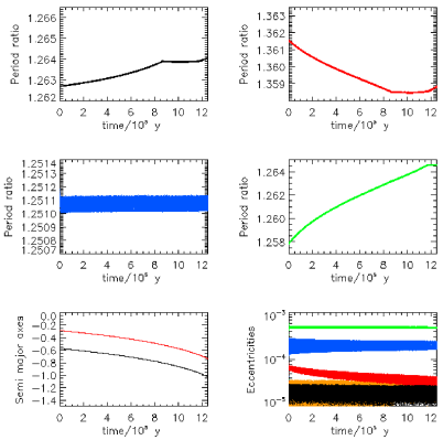
Figure 1: Time dependent evolution for run $sacd.$ The upper left panel shows the evolution of the ratio of the periods of planets 2 and planet 1 as a function of time. The corresponding plot for planet 3 and planet 2 is shown in the upper right panel, that for planet 4 and planet 3 is shown in the centre left panel and that for planet 5 and planet 4 in the centre right panel. The lower left panel shows the evolution of the logarithm of the semi-major axes of the innermost and outermost planets in units of $0.15AU$ as a function of time. The lower right panel shows the evolution of the eccentricities of planet 1 (black ), planet 2 (orange ) , planet 3 (green), planet 4 (blue curve) and planet 5 (red curve).

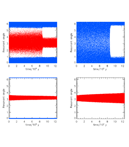
Figure 2: Time dependent evolution for run $sacd.$ The upper left panel shows the evolution of the resonant angles $5\lambda_{2}-4\lambda_{1}-\varpi_{1}$ (blue) and $5\lambda_{2}-4\lambda_{1}-\varpi_{2}$ (red). The upper right panel shows the evolution of the resonant angle $4\lambda_{3}-3\lambda_{2}-\varpi_{2}$ (blue). The lower left panel shows the evolution of the resonant angles $5\lambda_{4}-4\lambda_{3}-\varpi_{3}$ (blue) and $5\lambda_{4}-4\lambda_{3}-\varpi_{4}$ (red). The lower right panel shows the evolution of the resonant angle $5\lambda_{5}-4\lambda_{4}-\varpi_{5}$ (red).

5 Parameters of the simulations and application of the analytic model

We now indicate the setups and parameters associated with the models for which simulations were performed and the analytic theory was applied. The simulations were by means of N body calculations following the method outlined in eg. Papaloizou & Terquem (2001) (see also Papaloizou 2011, 2015). In all cases the system was assumed to be coplanar.

5.1 Initial semi-major axes and eccentricities

For the runs $sacd,$ denoted the standard case, $sacd_{1},$ $s_{1}ac_{1}f,$ $s_{1}ac_{1}f_{1},$ $sach$ and $sacm,$ apart from the eccentricities, orbital data for the five planets was taken from Campante et al. (2015) for Kepler 444. The period ratios of consecutive pairs moving from innermost to outermost are then $1.2627,1.3615,1.2511$ and $1.2579.$ These are close to 5:4, 4:3, 5:4 and 5:4 resonances respectively with relative separations of $1\%,2\%,0.09\%,$and $0.6\%$ respectively. The third and fourth planets are accordingly significantly closer to commensurability than the others. This semi-major axis setup is denoted by the label $a.$

For the run $sbcm$ the setup $a$ was modified such that consecutive planetary pairs, with the exception of $m_{3}$ and $m_{4}$ were moved closer to resonance, with relative separation reduced by a factor of $10.$ The period ratios of consecutive pairs were adjusted to become $1.2513,1.3360,1.2511$ and $1.2508.$ This was achieved by reducing the semi-major axes of planets 2, 3, 4 and 5 through multiplication by factors $0.993953,$ $0.981516,$ $0.981516$ and $0.977816$ respectively. The proximity to resonance becomes comparable for all pairs. This semi-major axis setup is denoted by the label $b.$

For the run $sb_{1}cd_{2},$ the setup $a$ was modified such that the semi-major axis of $m_{1}$ was increased by a factor $1.0061.$ This has the effect of contracting the system such that the innermost pair of planets starts closer to resonance (see below), This semi-major axis setup is denoted by the label $b_{1}.$

For all runs presented here the initial orbital eccentricities were assumed to be zero. In the case of Kepler 444 the observations are consistent with circular orbits though errors are large in the case of the outermost planet (see Van Eylen & Albrecht 2015). Note too that although the set up is for a specific set of semi-major axes, a standard scaling can be applied to allow results to apply to a setup where all the semi-major axes are scaled up or down by the same factor (see Section 5.3 below).

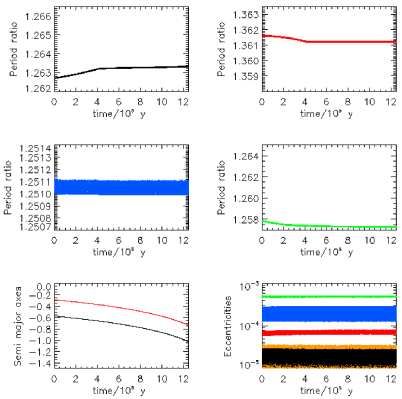
Figure 3: As in Fig. 1 but for run $sacd_{1}.$

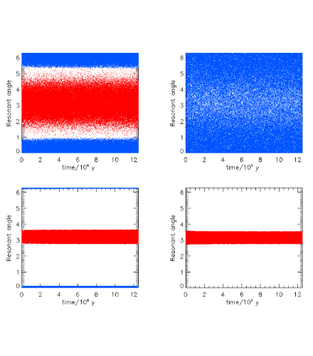
Figure 4: As in Fig. 2 but for run $sacd_{1}.$

5.2 Circularization times

Following the procedure outlined in Section 2.1 we adopt the disk model for which $t_{e,j}$ scales as $1/n_{j}$ or equivalently the orbital period of planet $j$ (see equation (5)). Migration times obtained from the analytic model of Section 4 will then scale in the same way. The standard circularization times $(c)$ we adopted for planet, $j,$ are given by

$$t_{e,j}=6.4\pi\times 10^{-4}(M/m_{j})/n_{j}.$$ (54)

This is equivalent to using (5) adopting a disk with a mass $5M_{J}$ within $1AU$ being a factor $5.6$ larger than expected from a minimum mass solar nebula. A disk this massive was adopted so as to obtain characteristic evolution times for the system $\sim 10^{6-7}y.,$ as conventionally expected for a protoplanetary disk lifetime, when the procedure to determine migration times described in Section 5.2.1 below was followed. Equation (54) was used in all cases except $s_{1}ac_{1}f$ and $s_{1}ac_{1}f_{1}$ for which the values obtained from this formula were increased by a factor of $100$ (see Table 1).

5.2.1 Migration times

The migration times for the runs $sacd,sach,sacm$ and $sbcm$ indicated in Table 1 and listed in Table 2 were determined from the analytic theory through the use of equations (46) - (48). In all cases excepting $sacm$ and $sbcm$ all consecutive pairs are assumed to interact resonantly with $p_{1}=p_{3}=p_{4}=4$ and $p_{2}=3.$ In addition $J=2$ so that only planets $3$ and $4$ are coupled by two first order resonances. This choice was made as planets $3$ and $4$ are the closest to resonance in the Kepler 444 system.

The cases $sacm$ and $sbcm$ were calculated assuming the system was composed of two separate independent subsystems as outlined in Section 4.3.1 above. In these cases planets $1$ and $2$ as well as planets $3$ and $4$ are coupled by a pair of first order resonances. We recall that migration times can be determined once the semi-major axes, masses and circularization times are specified, given a migration time for one of the planets in each subsystem, here taken to be the innermost one, assuming that the period ratios remain constant. More about the adopted masses and this procedure is indicated below.

The migration times for the run $s_{1}ac_{1}f$ listed in Table 2 were obtained from the set $d$ by reducing them by a factor of ten. This is to test the application of a simple scaling relation expected from the simplified analytic theory. The migration times for the runs $sacd_{1},$ $s_{1}ac_{1}f_{1}$ and $sb_{1}cd_{2}$ are labeled $d_{1},f_{1}$ and $d_{2}$ respectively and are listed in Table 3. These are obtained by slightly modifying values obtained from the analytic theory. Thus the times $d_{1}$ are obtained by heuristically adjusting those obtained from $d$ so as to reduce the magnitude of the evolution of the period ratios. The times $f_{1}$ are obtained from $f$ by increasing the migration time of the innermost planet by a factor $1.001.$ The times $d_{2}$ are obtained from $d$ by rescaling the migration time of the innermost planet so that was the same at its shifted position in $b_{1}$ as in its original position in $a.$ Note that the modification in the latter two cases only affects the migration time of the innermost planet.

5.2.2 Planet masses

As only planet radii are available and their densities are unknown, planet masses cannot be determined. In order to proceed we determined a set of planet masses by trial and error that were such that the product of the masses and migration times determined by application of the analytic model of Section 4, through use of equations (46) - (48) in Section 4.4 , for the standard run $sacd,$ were constant to within $\sim 3\%.$ This would be expected from the simplest migration calculations (eg. Papaloizou & Terquem 2006). In carrying out this procedure the migration time of the innermost planet, which was not otherwise determined, was chosen such that the system as a whole migrated significantly over an expected protoplanetary disk lifetime. Although the analytic model, through determination of the relative migration rates constrains the planet masses, we stress that the parameters we adopt are by no means unique but they enable investigation of the orbital architecture of a system resembling Kepler 444 and tests carried out for other examples not considered here have been found to lead to very similar conclusions.

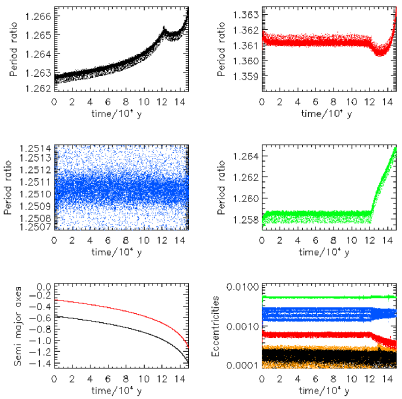
Figure 5: As in Fig. 1 but for run $s_{1}ac_{1}f$. Note that the range of eccentricities shown is an order of magnitude larger in this case.

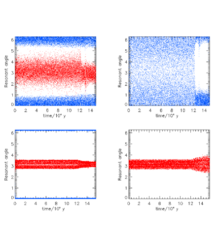
Figure 6: As in Fig. 2 but for run $s_{1}ac_{1}f.$

The standard masses chosen alongside the determination of migration times, using the analytic procedure described in Section (4.4), as indicated above, being denoted by the label $s,$ were $m_{1}~{}=~{}0.0546075M_{\oplus},$ $m_{2}~{}=~{}0.0689779M_{\oplus},$ $m_{3}~{}=~{}0.05333708M_{\oplus},$ $m_{4}~{}=~{}0.1348677M_{\oplus},$ and $m_{5}~{}=~{}0.1479524M_{\oplus}.$ Adopting the planetary radii given by Campante et al. (2015), the mean densities of the planets are then found to be $\rho_{j}/\rho_{\oplus}=0.853,0.562,0.369,0.829$ and $0.364$ for $j=1,2,3,4$ and $5$ respectively, indicating that they could be rocky bodies. We remark that these densities differ by a factor $\sim 2$ varying non monotonically with orbital separation. This type of non uniformity has been observed in the Kepler 11 system (Lissauer et al. 2011b) and the Kepler 138 system (Jontof-Hutter et al. 2015) and so should not be unexpected. Standard masses were adopted in all cases considered here except for $s_{1}ac_{1}f$ and $s_{1}ac_{1}f_{1}$ for which they were increased by by a factor of $10$ (see Table 1).

5.3 General scaling

Although the setups described above are for specific sets of semi-major axes, because the circularization and migration times we adopt are proportional to the orbital period, a standard scaling can be applied to expand the length scale of the initial setup. This simple scaling holds masses fixed while length scales are increased by a factor $\Lambda$ and times are increased by a factor $\Lambda^{3/2}.$ Thus results obtained for a given setup can be easily scaled to apply to an initial setup with an expanded length scale. This can also be arranged so that a given simulation is scaled to terminate close to the original setup.

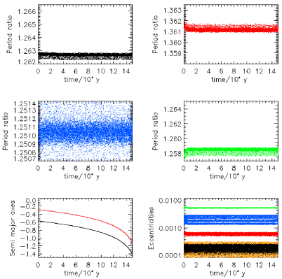
Figure 7: As in Fig. 1 but for run $s_{1}ac_{1}f_{1}.$ Note that the range of eccentricities shown is an order of magnitude larger in this case.

6 Simulation results

We now describe results for the standard case $sacd.$

6.1 The standard case $sacd$

For this case the initial semi-major axes and eccentricities were set up as indicated in Section 5.1 (see Table 1) and circularization times as indicated in Section 5.2. Migration times were determined as indicated in Section 5.2.1 and are given in Table 2. The planet masses are given in Section 5.2.2. We remark that the migration time of the innermost planet given in Table 2 is such that $t_{mig,1}/t_{e,1}=1.3\times 10^{5}.$ The expected value from the simplest migration calculations described in Sections 2 and 2.1 for which corotation torques do not play a significant role is $\sim(R/H)^{2}\sim 2.5\times 10^{3}$ which is smaller by a factor $\sim 54.$ This is an indication that modifications along the lines described in Section 2 may need to be invoked in order to slow down inward migration by between one and two orders of magnitude.

The time dependent evolution of the semi-major axes of the innermost and outermost planet is plotted in Fig. 1. The overall contraction of the system is by a factor of $\sim 3$ for a run time of $1.25\times 10^{6}y.$ Note that the system can be scaled to start at initial radii a factor of two larger by increasing the times by a factor $2^{3/2},$ then finishing near to the initial set up. The time dependent evolution of ratio of the period ratios of planet 2 and planet 1, planet 3 and planet 2, as well as planet 4 and planet 5 are also shown in Fig. 1 as is the time dependent evolution of the eccentricities.

The eccentricities obtained from the analytic model were $e_{1}=2.01\times 10^{-5},e_{2}=7.41\times 10^{-6},e_{3}=4.81\times 10^{-4},e_{4}=2.04\times 10^{-4},$ and $e_{5}=6.70\times 10^{-5}.$ These are in reasonable agreement with the mean values seen at early times for simulation $sacd$ and at all times for simulation $sabcd_{1}$ described below for which mean values of the eccentricities show less variation. These small values are also in line with the near circular orbits inferred from the observations by Van Eylen & Albrecht (2015).

The quantity ${\cal C}_{N,1}=(1/t_{mig,N}-1/t_{mig,1})t_{mig,1}$ is a measure of the rate of convergence of the entire system. For the run $sabc,$ ${\cal C}_{N,1}=7\times 10^{-3}$ (see Table 2). This means that a scale contraction of order unity is associated with a relative contraction of only around $1\%.$ This is a consequence of the relatively wide separation of consecutive pairs from resonance. From equation (45) it follows that ${\cal C}_{N,1}$ scales as the squares of the eccentricities which themselves are approximately inversely proportional to the separation from resonance (see equations (52) and (53) ). Thus in order to obtain a faster rate of convergence of the system, enabling significant convergence during the evolution, from our analysis the system would have had to have been closer to resonance. Only in the late stages of evolution could the migration times increase to produce conditions like those of $sacd.$

The time dependent evolution of the resonant angles $5\lambda_{2}-4\lambda_{1}-\varpi_{1},$ $5\lambda_{2}-4\lambda_{1}-\varpi_{2},$ $4\lambda_{3}-3\lambda_{2}-\varpi_{2},$ $5\lambda_{4}-4\lambda_{3}-\varpi_{3},$ $5\lambda_{4}-4\lambda_{3}-\varpi_{4}$ and $5\lambda_{5}-4\lambda_{4}-\varpi_{5}$ is shown in Fig. 2. All of these angles, except the second connecting planets $1$ and $2,$ contribute in the analytic theory and apart from that one, they are all seen to librate at early times except for $4\lambda_{3}-3\lambda_{2}-\varpi_{2}.$ This angle circulates. In addition although the angle, $5\lambda_{2}-4\lambda_{1}-\varpi_{2},$ circulates at early times as expected according to the analytic model of Section 4 (see discussion in Section 4.3 below equation (28) and also in Sections 4.3.1 and 5.2.1), it does not do so uniformly indicating that it may contribute to the evolution. The last two features indicate that at this stage, planets $1$ and $2$ are not as strongly coupled to the rest as in the simple analytic theory, a feature further investigated below. This may be related to the fact that planets $2$ and $3$ are the most widely separated from resonance. Resonant angles not illustrated in Fig. 2 always circulate.

The deviation of the period ratio of planets $4$ and $5$ from strict resonance increases by a factor $\sim 1.8$ during the run. Corresponding to this change the mean eccentricity of planet $5$ decreases by approximately the same factor as expected from equation (53) when the circularization time there is assumed to be arbitrarily large. The deviation of the period ratio of planets $1$ and $2$ from resonance increases by $\sim 10^{-3}$ corresponding to a relative increase of $\sim 8\%.$ The mean eccentricity of planet $1$ is seen to decrease by a corresponding amount as indicated by equation (52). The deviation of the period ratio of planets $2$ and $3$ from resonance decreases by $\sim 2\times 10^{-3},$ over the run time. However, this deviation as well as that associated with planets $1$ and $2$ stop their secular advance at a time $\sim 8.5\times 10^{5}y.,$ at which point a Laplace resonance between planets $1,$ $2$ and $3$ is formed. This is indicated by the fact that after that the angles $4\lambda_{3}-3\lambda_{2}-\varpi_{2}$ and $5\lambda_{2}-4\lambda_{1}-\varpi_{2}$ both then clearly librate. The period ratio of planets $3$ and $4$ being the closest to resonance remains essentially unchanging throughout the evolution. The period ratio of planets $4$ and $5$ increases throughout, stabilizing only at the end of the simulation, the deviation from resonance having increased by $\sim 5\times 10^{-3}.$ The setting up of a Laplace resonance was not anticipated in the analytic treatment. However, we found that small adjustments to the input migration times could result in much smaller changes to the period ratios, so avoiding the formation of a Laplace resonance.

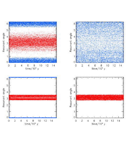
Figure 8: As in Fig. 2 but for run $s_{1}ac_{1}f_{1}$.

6.1.1 The modified standard case $sacd_{1}$

In this case the initial setup and initial conditions were the same as for $sacd,$ the only difference was that the input migration times were slightly adjusted (see Section 5.2.1). The modified values are listed in Table 3. In this case the simulation underwent the same amount of radial contraction but the period ratios underwent much less evolution. The maximum deviation from resonance changing by less than $5\times 10^{-4}$ in all cases. These features are illustrated in Fig. 3. The evolution of the resonant angles illustrated in Fig. 4 is similar to that found for $sacd$ at early times. But in this case the variation of the period ratios is insufficient for a Laplace resonance to form and so the character of the evolution of the resonant angles does not change.

Although these simulations indicate that it is possible to set up the system such that convergent migration and circularization are balanced. The wide separations from resonance characteristic of Kepler 444 indicate only very weak convergence. This means that if the system is not formed very close to it’s final period ratio configuration, the migration times assumed for $sacd_{1}$ could only apply in the final evolutionary stages.

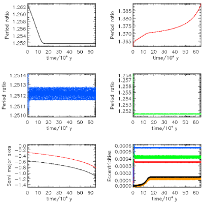
Figure 9: As in Fig. 1 but for run $sach.$

6.2 Simulations with larger masses

According to the analytic discussion in Sections 4 and 4.4, when the planet masses are increased by a factor, $F_{m},$ and the expression for the circularization time given by equation (54) is scaled by a factor $F_{c},$ the eccentricities scale as $F_{m}$ as long as the inverse circularization time in the denominators of equations (52) and (53) is neglected, the latter being a good approximation. The calculated convergent migration rates then scale as $F_{m}^{3}/F_{c}.$ Thus if all masses are scaled by a factor of $10$ and $F_{c}=100,$ calculated migration times should consistently decrease by a factor of $10.$

In order to test this scaling we performed run $s_{1}ac_{1}f$ for which the input data for run $sacd$ was scaled as indicated above. Planet masses were increased by a factor of $10,$ migration times were reduced by a factor of $10$ and $F_{c}=100$ see Tables 1 and 2.

The time dependent evolution of the semi-major axes of the innermost and outermost planet and the period ratios is illustrated in Fig. 5. The overall contraction of the system is by a factor of $\sim 3$ after a time $1.25\times 10^{5}y.$ consistent with the migration time reduction expected when compared to run $sacd.$ Note that as for that case, the system can be scaled to start at larger initial radii by appropriately increasing the times so that the system then finishes near to the initial set up. In this case, with the exception of the innermost pair, the period ratios of consecutive pairs on average remain constant up and till $1.2\times 10^{5}y.$ This indicates that the innermost pair are more strongly coupled than in the analytic model which appears to work better for the other planet pairs in this case. Up till this time the innermost period ratio increases steadily until the deviation from resonance is $\sim 2\times 10^{-3}.$ Then, once the conditions for it are satisfied, a Laplace resonance is set up as for the run $sacd.$ After this, the period ratio deviation from resonance of planets $2$ and $3$ and also $4$ and $5$ increase, the latter by up to $5\times 10^{-3}.$ The time dependent evolution of the resonant angles corresponding to those for the run $sacd$ shown in Fig.2 is shown in Fig. 6. The evolution of all angles is qualitatively very similar in these two cases. However, the Laplace resonance is set up after $1.2\times 10^{5}y.$ which is somewhat later than the expected scaled time of $8\times 10^{4}y.$ When this occurs the angle $4\lambda_{3}-3\lambda_{2}-\varpi_{2}$ starts to librate causing the form of the evolution to change. Planets $2$ and $3$ become more strongly coupled , affecting planet $4$ through the strong resonance between planets $3$ and $4,$ and hence the period ratio of planets $4$ and $5.$ The overall effect of the increased resonant coupling is that the system separates.

6.2.1 Reducing the migration rate of the innermost planet

The Laplace resonance was set up in the run $s_{1}ac_{1}f$ because of the evolving period ratio of the innermost pair of planets. In order to counteract this and obtain more stable period ratios we repeated the simulation with the migration time of the inner planet increased by a factor $1.001$ in simulation $s_{1}ac_{1}f_{1}.$ The evolution of the period ratios plotted in Fig. 7 shows that the period ratio deviations from resonance change by less than $\sim 5\times 10^{-4}$ in all cases with no Laplace resonance being set up. The time dependent evolution of the resonant angles corresponding to those shown for the run $sacd_{1}$ is shown in Fig.8, the character of the evolution being very similar. Although the simulations for larger planet masses show similar features to those with lower masses, there is not a precise scaling between the two most likely because the simple analytic model does not give a completely accurate description for the behaviour of the resonant angles.

6.3 Simulations with closer commensurabilities

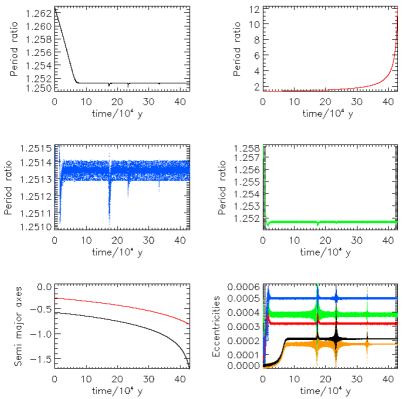
Figure 10: As in Fig. 1 but for run $sacm.$

Although we have been able to obtain migrating systems with only a small variation of period ratios, on account of the deviations from resonances being too large, the inferred rates of convergent migration are very small implying the system cannot have been brought together from a wide separation. Such a situation could only apply during the late evolutionary stages. In order to study systems with faster relative migration rates we have performed simulations $sach,$ $sacm$ and $sbcm$ which have systems with consecutive pairs, except for planets $3$ and $4,$ an order of magnitude closer to resonance than those considered above.

In order to obtain migration times from the analytic method of Section 4 for these, the initial semi-major axes of consecutive pairs were adjusted so that the deviations of all consecutive pairs of planets from resonance became $\leq 2\times 10^{-3}$ as indicated in Section 5.1 for the procedure labelled $b.$ For these simulations, for simplicity we retain the same planet masses as in the standard case even though the dependence on migration time is changed. We note that this could be adjusted by adjusting the relative separations from resonance for the different planets.

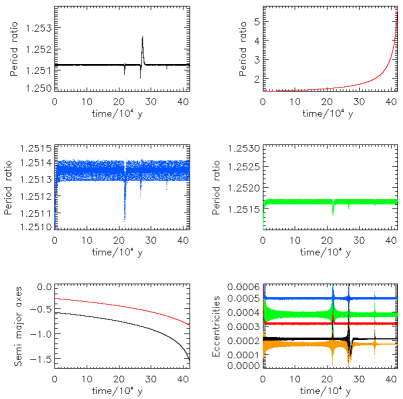
Figure 11: As in Fig. 1 but for run $sbcm.$

6.3.1 Simulations with migration rates obtained assuming all consecutive pairs are coupled

The migration times obtained following the procedure for this case outlined in Section 4.3.1 labelled, $h,$ are tabulated in Table 1. However, when performing the simulation $sach,$ , the semi-major axes were initiated as in procedure $a$ (see Section 5.1). The consequence of that in this case is that the period ratios adjust to become closer to resonance. The relative convergence parameter ${\cal C}_{N,1}=0.3$ indicating that a significant relative contraction can occur while the system contracts as a whole. The time dependent evolution of the semi-major axes of the innermost and outermost planet and the period ratios is plotted in Fig. 9. The overall contraction of the system is by a factor of $\sim 3$ after a time $6.5\times 10^{5}y.$ In this case the period ratios for the innermost and outermost pairs of planets move rapidly closer to resonance as expected. However, the period ratio of planets $2$ and $3$ continually increases up to $1.39$ indicating that the inner two planets decouple from the outer $3$ as indicated above. This is supported by the behaviour of the resonant angles which all librate except for those connecting planets $2$ and $3.$ Accordingly we go on to consider simulations for which the migration times are calculated assuming this decoupling occurs.

6.3.2 Migration rates obtained assuming inner two and outer three planets behave as separate systems

The migration times obtained following the procedure for this case outlined in Section 4 are labelled, $m$ and are tabulated in Table 1. As indicated in Section 4.3.1 in order to obtain these, the migration times for both planet 1 and planet 3 should be specified. This determines how the separate subsystems separate. To obtain a working model we specified $t_{mig,3}=0.8t_{mig,1}.$ When performing the simulation $sacm,$ the semi-major axes were initiated as in procedure $a.$ On the other hand, when performing the simulation $sbcm,$ the semi-major axes were initiated as in procedure $b$ as used for the analytic calculation of the migration times. The relative convergence parameter ${\cal C}_{N,1}=0.35$ for the innermost pair which is significant. The time dependent evolution of the semi-major axes of the innermost and outermost planet and the period ratios for $sacm$ is plotted in Fig. 10. The corresponding quantities for $sbcm$ are plotted in Fig. 11. Apart from planets $2$ and $3$ the period ratios move closer to resonance for $sacm$ but remain approximately constant for $sbcm.$ The period ratio of planets $2$ and $3$ increases dramatically up to $5$ for $sacm$ and $10$ for $sbcm$ indicating a more serious decoupling of the two subsystems than for $sach.$ However, the large increase in this period results in successive passage through 3:2, 5:3 and 2:1 resonances which are indicated by the spikes seen in time dependent evolution of the period ratios. The behaviour of the resonant angles for both simulations is very similar to that seen in $sach.$

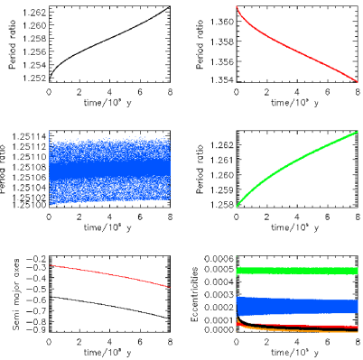
Figure 12: As in Fig. 1 but for run $sb_{1}cd_{2}.$

6.3.3 The innermost planet moved closer to resonance

The above simulations indicate the system should have been closer to resonance than currently observed in Kepler 444 if significant convergent migration has occurred. To attain a situation like that in Kepler 444, the migration times would have to increase to attain values like those in setup $a,$ at which point little further convergence occurs. In order to investigate whether such adjustments can occur we performed simulation $sb_{1}cd_{2}.$ This had semi-major axes set up as in $sacd$ but the semi-major axis of the innermost planet then increased such that the period ratio of planets $1$ and $2$ was the same as for set up $b.$ The migration time of the innermost planet was then scaled such that it took on the same value as in $sacd,$ but at its new position. The time dependent evolution of the semi-major axes of the innermost and outermost planet and the period ratios for $sb_{1}cd_{2}$ are plotted in Fig. 12. The period ratio for planets $1$ and $2$ increases to the current value after $8\times 10^{5}y.$ However the period ratio of the outermost pair also increases significantly while the period ratio of planets $2$ and $3$ decreases significantly. Although the above does not represent a precise modelling, it does indicate that expansion to present period ratios from ones closer to resonance is a possibility.

7 Discussion

In this paper we have studied the evolution of multi-planet systems in which the components undergo tidal interaction with a protoplanetary disk with reference to a system with architecture resembling that of Kepler 444.

We formulated an analytic model for a planetary system with consecutive pairs in resonance undergoing orbital circularization and orbital migration as a unit in Section 4. The system as a whole could be considered as a unit, or it could be considered to be composed of independent subsystems with the analysis being applied to each separately. The interaction between neighbours is supposed to occur through the influence of either one or two retained resonant angles. For a system or subsystem in which such commensurabilities are maintained, the model enables the migration times for each planet to be determined once planet masses, circularization times and the migration time for the innermost planet is specified. The latter was chosen so that the time scale for the evolution of the system was in the range of $10^{6-7}y.$ as expected for current protoplanetary disks. However, in doing this we required a disk model with mass exceeding that for a minimum mass solar nebula by a factor $\sim 5.6$ in its inner regions within $1AU.$ But note that there is no implication from this concerning the mass distribution at large distances.

The planet masses for systems such as Kepler 444 are very uncertain as only their radii are known. To obtain a working model we specified values for the masses such that the migration times for the standard case were approximately inversely proportional to the planet mass as expected from the simple theory of disk planet interaction. Migration times and masses determined from these procedures, along with circularization times and the current orbital architecture of Kepler 444 were used as input data for detailed numerical simulations. But it is important to note that results may be scaled so that the initial systems start at an expanded length scale and finish in configuration resembling the original one (see Section 5.3).

Because of relatively large deviations from exact resonance, the migration times found in this way for the standard case and other cases with the same relative separation from resonances are such that they would produce weak convergent migration of the system, contracting by only $\sim 1\%$ while undergoing significant migration as a whole (see Sections 6.1 and 6.2). Such migration rates are also between one and two orders of magnitude smaller than expected from the simplest modelling of disk-planet interaction indicating that significant modification along the lines indicated in Section 2 is needed.

This means that the system is unlikely to have reached the current architecture from a state where it’s components were significantly more widely separated. In that case these inferred migration rates could have only applied during the later evolutionary phases.

Simulations of the standard case $sacd$ and $s_{1}ac_{1}f$ presented in Sections 6.1 and 6.2 show only a weak coupling between planets $2$ and $3$ on account of their relatively large separation from resonance, indicating a tendency of the inner two planets to be decoupled from the outer $3.$ Although period ratios did not remain strictly constant during the evolution such that Laplace resonances could eventually form, we found that relatively small adjustments to the migration times obtained from the analytic model could significantly reduce the variation of the period ratios such that this did not occur.

In order to study systems showing stronger convergent migration we studied systems with consecutive pairs, not including planets $3$ and $4,$ an order of magnitude relatively closer to resonance than in the standard case. These can then show significant relative convergence on the time scale for which the system contracts as a whole. However, we found again that the inner two planets tended to become detached from the outer $3.$ This happened for migration times determined from the analytic model independently of whether they were obtained assuming the system was split into two separate subsystems or not (see Sections 6.3.1 and 6.3.2).

These simulations confirm the view that if the system underwent significant convergent migration before reaching the final state the resonances were closer and the migration times shorter during this phase. One could speculate that migration rates slowed and resonances moved apart as the system approached the inner regions of the disk where a process causing its truncation operated. The latter evolution is similar to that obtained when tidal interaction with a central star causes orbital circularization in the absence of orbital migration (Papaloizou 2011; Lithwick & Wu 2012; Batygin & Morbidelli 2013).

Finally we remark that our pilot studies are incomplete as they were only carried out in order to investigate the potential importance of orbital migration and circularization induced by the tidal interaction of a planetary system, such as Kepler 444, with a protoplanetary disk modelled in the simplest possible way. We have only considered processes occurring when the system is not too far removed from its final configuration and not addressed the issue of possible migration from large distances. Furthermore potentially important processes such as stochastic forces resulting from disk turbulence or planetesimal migration, which could occur during the period for which the evolution was studied and also after the gas disk has dispersed, have been omitted. Nonetheless they indicate that the effects we study could potentially play an important role in producing the current architecture.

References

- (1) Baruteau, C.. Crida, A., Paardekooper, S.-J., Masset, F., Guilet, J., Bitsch, B., Nelson, R., Kley, W., Papaloizou, J.: Planet-Disk Interactions and Early Evolution of Planetary Systems. Protostars and Planets VI. pp. 667-689. University of Arizona Press, Tucson (2014)
- (2) Batalha, N. M., Rowe, J. F., Bryson, S. T., et al. : Planetary Candidates Observed by Kepler. III. Analysis of the First 16 Months of Data. Astrophys J Supp S. 204, id. 24, 21 pp. (2013)
- (3) Batygin, K., Morbidelli, A.: Dissipative Divergence of Resonant Orbits. Astron J. 145, id. 1, 10 pp. (2013)
- (4) Benitez-Llambay, P., Masset, F., Koenigsberger, G., Szulagyi, J.: Planet heating prevents inward migration of planetary cores. Nature 520, 63-65 (2015)
- (5) Brouwer, D., Clemence, G.M.: Methods of Celestial Mechanics. pp. 416-421. Academic Press, New York (1961)
- (6) Campante, T.L. et al.: An Ancient Extrasolar System with Five Sub-Earth-size Planets. Astrophys J. 799, id. 170, 17 pp. (2015)
- (7) Correa-Otto, J., Michtchenko, T. A., Beaugé, C.: A new scenario for the origin of the 3/2 resonant system HD 45364. Astron Astrophys., 560, id. A65, 10 pp. (2013)
- (8) Cresswell, P., Nelson, R.P.: On the evolution of multiple protoplanets embedded in a protostellar disc. Astron Astrophys. 450, 833-853 (2006)
- (9) Goldreich P., Soter S.: Q in the Solar System. Icarus. 5, 375-389 (1966)
- (10) Guilet, J., Baruteau, C., Papaloizou, J. C. B.: Type I planet migration in weakly magnetized laminar disks. Mon. Not. R. Astron. Soc. 430, 1764 -1783 (2013)
- (11) Ida, S., & Lin, D. N. C.: Toward a Deterministic Model of Planetary Formation. IV. Effects of Type I Migration. Astrophys J. 673, 487-501 (2008)
- (12) Jontof-Hutter, D., Rowe, J. F., Lissauer, J. J., Fabrycky, D. C., Ford, E. B.: The mass of the Mars-sized exoplanet Kepler-138 b from transit timing. Nature 522, 321-323 (2015)
- (13) Lissauer, J. J., Fabrycky, D. C., Ford, E. B., et al.: A closely packed system of low-mass, low-density planets transiting Kepler-11. Nature 470, 53-58 (2011)b
- (14) Lissauer, J. J., Ragozine,D., Fabrycky, D. C., et al.: Architecture and Dynamics of Kepler’s Candidate Multiple Transiting Planet Systems. Astrophys J Suppl S. 197, id. 8, 26 pp. (2011)a
- (15) Lithwick, Y., Wu, Y.: Resonant Repulsion of Kepler Planet Pairs. Astrophys J. 756, id. L11, 5 pp. (2012)
- (16) Murray, C.D., Dermott, S.F.: Solar System Dynamics. pp. 254-255. Cambridge University Press, Cambridge (1999)
- (17) Nelson, R.P., Papaloizou, J.C.B.: The interaction of a giant planet with a disc with MHD turbulence - II. The interaction of the planet with the disc. Mon. Not. R. Astron. Soc. 350, 849-864 (2004)
- (18) Ogihara, M., Morbidelli, A., Guillot, T.: Suppression of type I migration by disk winds. Astron Astrophys. 584, id. L1, 4pp. (2015)
- (19) Paardekooper S.–J, Mellema G.: Halting type I planet migration in non-isothermal disks. Astron Astrophys. 459, L17-L20 (2006)
- (20) Paardekooper, S.-J., Papaloizou, J.C.B.: On corotation torques, horseshoe drag and the possibility of sustained stalled or outward protoplanetary migration. Mon. Not. R. Astron. Soc. 394, 2283-2296 (2009)
- (21) Papaloizou J. C. B.: Global m = 1 modes and migration of protoplanetary cores in eccentric protoplanetary discs. Astron Astrophys. 388, 615-631 (2002)
- (22) Papaloizou, J.C.B.: Disc-planet interactions: migration and resonances in extrasolar planetary systems. Celest. Mech. Dyn. Astron. 87, 53-83 (2003)
- (23) Papaloizou, J.C.B.: Tidal interactions in multi-planet systems. Celest. Mech. Dyn. Astron. 111, 83-103 (2011)
- (24) Papaloizou J. C. B.: Three body resonances in close orbiting planetary systems: tidal dissipation and orbital evolution. International Journal of Astrobiology 14, 291-304 (2015)
- (25) Papaloizou, J.C.B., Szuszkiewicz, E.: On the migration-induced resonances in a system of two planets with masses in the Earth mass range. Mon. Not. R. Astron. Soc. 363, 153-176 (2005)
- (26) Papaloizou, J.C.B., Terquem, C.: Dynamical relaxation and massive extrasolar planets. Mon. Not. R. Astron. Soc. 325, 221-230 (2001)
- (27) Papaloizou J.C.B., Terquem C.: Planet formation and migration. Rep. Prog. Phys. 69, pp. 119-180 (2006)
- (28) Papaloizou, J.C.B., Terquem, C.: On the dynamics of multiple systems of hot super-Earths and Neptunes: tidal circularization, resonance and the HD 40307 system. Mon. Not. R. Astron. Soc. 405, 573-592 (2010)
- (29) Podlewska-Gaca, E., Papaloizou, J. C. B., Szuszkiewicz, E.: Outward migration of a super-Earth in a disc with outward propagating density waves excited by a giant planet. Mon. Not. R. Astron. Soc. 421, 1736-1756 (2012)
- (30) Raymond, S.N., Barnes, R., Mandell, A.M.: Observable consequences of planet formation models in systems with close-in terrestrial planets. Mon. Not. R. Astron. Soc. 384, 663-674 (2008)
- (31) Sinclair, A.T.: The orbital resonance amongst the Galilean satellites of Jupiter. Mon. Not. R. Astron. Soc. 171, 59-72 (1975)
- (32) Steffen, J. H., Fabrycky, D. C., Agol, E. , et al.: Transit timing observations from Kepler - VII. Confirmation of 27 planets in 13 multiplanet systems via transit timing variations and orbital stability. Mon. Not. R. Astron. Soc. 428, 1077-1087 (2013)
- (33) Suzuki, T. K., Muto, T., & Inutsuka, S.: Astrophys J. Protoplanetary Disk Winds via Magnetorotational Instability: Formation of an Inner Hole and a Crucial Assist for Planet Formation. Astrophys J. 718, 1289 -1304 (2010)
- (34) Tanaka, H., Takeuchi, T., Ward, W. R.: Three-Dimensional Interaction between a Planet and an Isothermal Gaseous Disk. I. Eccentricity Waves and Bending Waves. Astrophys J. 602, 388-395 (2004)
- (35) Terquem, C. E. J. M. L. J. : Stopping inward planetary migration by a toroidal magnetic field. Mon. Not. R. Astron. Soc. 341, 1157-1173 (2003)
- (36) Terquem, C., Papaloizou, J.C.B.: Migration and the formation of systems of hot super-Earths and Neptunes. Astrophys. J. 654, 1110-1120 (2007)
- (37) Van Eylen, V., Albrecht, S.: Eccentricity from Transit Photometry: Small Planets in Kepler Multi-planet Systems Have Low Eccentricities. Astrophys J. 808, 126-145 (2015)
- (38) Ward, W.R.: Protoplanet migration by Nebula tides. Icarus 126, 261-281 (1997)