Dictionary Learning for Massive Matrix Factorization

Abstract

Sparse matrix factorization is a popular tool to obtain interpretable data decompositions, which are also effective to perform data completion or denoising. Its applicability to large datasets has been addressed with online and randomized methods, that reduce the complexity in one of the matrix dimension, but not in both of them. In this paper, we tackle very large matrices in both dimensions. We propose a new factorization method that scales gracefully to terabyte-scale datasets. Those could not be processed by previous algorithms in a reasonable amount of time. We demonstrate the efficiency of our approach on massive functional Magnetic Resonance Imaging (fMRI) data, and on matrix completion problems for recommender systems, where we obtain significant speed-ups compared to state-of-the art coordinate descent methods.

Matrix factorization is a flexible tool for uncovering latent factors in low-rank or sparse models. For instance, building on low-rank structure, it has proven very powerful for matrix completion, e.g. in recommender systems (Srebro et al., 2004; Candès & Recht, 2009). In signal processing and computer vision, matrix factorization with a sparse regularization is often called dictionary learning and has proven very effective for denoising and visual feature encoding (see Mairal, 2014, for a review). It is also flexible enough to accommodate a large set of constraints and regularizations, and has gained significant attention in scientific domains where interpretability is a key aspect, such as genetics and neuroscience (Varoquaux et al., 2011).

As a widely-used model, the literature of matrix factorization is very rich and two main classes of formulations have emerged. The first one addresses an optimization problem involving a convex penalty, such as the trace or max norms (Srebro et al., 2004). These penalties promote low-rank structures, have strong theoretical guarantees (Candès & Recht, 2009), but they do not encourage sparse factors and lack scalability for very-large datasets. For these reasons, our paper is focused on a second type of approach, that relies on nonconvex optimization. Specifically, the motivation of our work originally came from the need to analyze huge-scale fMRI datasets, and the difficulty of current algorithms to process them.

To gain scalability, stochastic (or online) optimization methods have been developed; unlike classical alternate minimization procedures, they learn matrix decompositions by observing a single matrix column (or row) at each iteration. In other words, they stream data along one matrix dimension. Their cost per iteration is significantly reduced, leading to faster convergence in various practical contexts. More precisely, two approaches have been particularly successful: stochastic gradient descent (see Bottou, 2010) has been widely used in recommender systems (see Bell & Koren, 2007; Rendle & Schmidt-Thieme, 2008; Rendle, 2010; Blondel et al., 2015, and references therein), and stochastic majorization-minimization methods for dictionary learning with sparse and/or structured regularization (Mairal et al., 2010; Mairal, 2013). Yet, stochastic algorithms for dictionary learning are currently unable to deal efficiently with matrices that are large in both dimensions.

In a somehow orthogonal way, the growth of dataset size has proven to be manageable by randomized methods, that exploit random projections (Johnson & Lindenstrauss, 1984; Bingham & Mannila, 2001) to reduce data dimension without deteriorating signal content. Due to the way they are generated, large-scale datasets generally have an intrinsic dimension that is significantly smaller than their ambient dimension. Biological datasets (McKeown et al., 1998) and physical acquisitions with an underlying sparse structure enabling compressed sensing (Candès & Tao, 2006) are good examples. In this context, matrix factorization can be performed by using random summaries of coefficients. Recently, those have been used to compute PCA (Halko et al., 2009), a classical matrix decomposition technique. Yet, using random projections as a pre-processing step is not appealing in our applicative context since the factors learned on reduced data loses interpretability.

Main contribution.

In this paper, we propose a dictionary learning algorithm that (i) scales both in the signal dimension (number of rows) and number of signals (number of columns), (ii) deals with various structured sparse regularization penalties, (iii) handles missing values, and (iv) provides an explicit dictionary with easy interpretation. As such, it is non-trivial extension of the online dictionary learning method of Mairal et al. (2010), where, at every iteration, signals are partially observed with a random mask, and with low-complexity update rules that depend on the (small) mask size instead of the signal size.

To the best of our knowledge, our algorithm is the first that enjoys all aforementioned features; in particular, we are not aware of any other dictionary learning algorithm that is scalable in both matrix dimensions. For instance, Pourkamali-Anaraki et al. (2015) use random projection with k-SVD, a batch dictionary learning algorithm (Aharon et al., 2006) that does not scale well in the number of training signals. Online matrix decomposition in the context of missing values was also proposed by Szabó et al. (2011), but without scalability in the signal (row) size.

On a massive fMRI dataset (2TB, $n=2.4\cdot 10^{6}$, $p=2\cdot 10^{5}$), we were able to learn interpretable dictionaries in about 10 hours on a single workstation, an order of magnitude faster than the online approach of Mairal et al. (2010). On collaborative filtering experiments, where sparsity is not needed, our algorithm performs favorably well compared to state-of-the-art coordinate descent methods. In both experiments, benefits for the practitioner were significant.

1 Background on Dictionary Learning

In this section, we introduce dictionary learning as a matrix factorization problem, and present stochastic algorithms that observe one column (or a minibatch) at every iteration.

1.1 Problem Statement

The goal of matrix factorization is to decompose a matrix ${\mathbf{X}}\in{\mathbb{R}}^{p\times n}$ – typically $n$ signals of dimension $p$ – as a product of two smaller matrices:

$${\mathbf{X}}\approx{\mathbf{D}}{\mathbf{A}}\quad\text{with}\quad{\mathbf{D}}\in{\mathbb{R}}^{p\times k},\;{\mathbf{A}}\in{\mathbb{R}}^{k\times n},$$ (1)

with potential sparsity or structure requirements on ${\mathbf{D}}$ and ${\mathbf{A}}$. In statistical signal applications, this is often a dictionary learning problem, enforcing sparse coefficients ${\mathbf{A}}$. In such a case, we call ${\mathbf{D}}$ the “dictionary” and ${\mathbf{A}}$ the sparse codes. We use this terminology throughout the paper.

Learning the dictionary is typically performed by minimizing a quadratic data-fitting term, with constraints and/or penalties over the code and the dictionary:

$$\min_{\begin{subarray}{c}{\mathbf{D}}\in\mathcal{C}\\ {\mathbf{A}}=[\boldsymbol{\alpha}_{1},\ldots,\boldsymbol{\alpha}_{n}]\in{\mathbb{R}}^{k\times n}\end{subarray}}\sum_{i=1}^{n}\frac{1}{2}\bigl{\|}{\mathbf{x}}_{i}-{\mathbf{D}}\boldsymbol{\alpha}_{i}\bigr{\|}_{2}^{2}+\lambda\,\Omega(\boldsymbol{\alpha}_{i}),$$ (2)

where $\mathcal{C}$ is a convex set of ${\mathbb{R}}^{p\times k}$, and a $\Omega:{\mathbb{R}}^{p}\rightarrow{\mathbb{R}}$ is a penalty over the code, to enforce structure or sparsity. In large $n$ and large $p$ settings, typical in recommender systems, this problem is solved via block coordinate descent, which boils down to alternating least squares if regularizations on ${\mathbf{D}}$ and $\boldsymbol{\alpha}$ are quadratic (Hastie et al., 2014).

Constraints and penalties.

The constraint set $\mathcal{C}$ is traditionally a technical constraint ensuring that the coefficients $\boldsymbol{\alpha}$ do not vanish, making the effect of the penalty $\Omega$ disappear. However, other constraints can also be used to enforce sparsity or structure on the dictionary (see Varoquaux et al., 2013). In our paper,$\mathcal{C}$ is the Cartesian product of a $\ell_{1}$ or $\ell_{2}$ norm ball:

$$\mathcal{C}=\{{\mathbf{D}}\in{\mathbb{R}}^{p\times k}~{}~{}~{}\text{s.t.}~{}~{}~{}\psi({\mathbf{d}}_{j})\leq 1\quad\forall j=1,\ldots,k\},$$ (3)

where ${\mathbf{D}}=[{\mathbf{d}}_{1},\ldots,{\mathbf{d}}_{k}]$ and $\psi=\|\cdot\|_{1}$ or $\psi=\|\cdot\|_{2}$. The choice of $\psi$ and $\Omega$ typically offers some flexibility in the regularization effect that is desired for a specific problem; for instance, classical dictionary learning uses $\psi=\|\cdot\|_{2}$ and $\Omega=\|\cdot\|_{1}$, leading to sparse coefficients $\boldsymbol{\alpha}$, whereas our experiments on fMRI uses $\psi=\|\cdot\|_{1}$ and $\Omega=\|\cdot\|_{2}^{2}$, leading to sparse dictionary elements ${\mathbf{d}}_{j}$ that can be interpreted as brain activation maps.

1.2 Streaming Signals with Online Algorithms

In stochastic optimization, the number of signals $n$ is assumed to be large (or potentially infinite), and the dictionary ${\mathbf{D}}$ can be written as a solution of

$$\min_{{\mathbf{D}}\in\mathcal{C}}\;f({\mathbf{D}})\quad\text{where}\quad f({\mathbf{D}})={\mathbb{E}}_{\mathbf{x}}\bigl{[}l({\mathbf{x}},{\mathbf{D}})\bigr{]}$$ (4)

$$\quad l({\mathbf{x}},{\mathbf{D}})=\min_{\boldsymbol{\alpha}\in{\mathbb{R}}^{k}}\frac{1}{2}\|{\mathbf{x}}-{\mathbf{D}}\boldsymbol{\alpha}\|_{2}^{2}+\lambda\,\Omega(\boldsymbol{\alpha}),$$

where the signals ${\mathbf{x}}$ are assumed to be i.i.d. samples from an unknown probability distribution. Based on this formulation, Mairal et al. (2010) have introduced an online dictionary learning approach that draws a single signal ${\mathbf{x}}_{t}$ at iteration $t$ (or a minibatch), and computes its sparse code $\boldsymbol{\alpha}_{t}$ using the current dictionary ${\mathbf{D}}_{t-1}$ according to

$$\boldsymbol{\alpha}_{t}\leftarrow\operatornamewithlimits{\mathrm{argmin}}_{\boldsymbol{\alpha}\in{\mathbb{R}}^{k}}\frac{1}{2}\|{\mathbf{x}}_{t}-{\mathbf{D}}_{t-1}\boldsymbol{\alpha}\|^{2}_{2}+\lambda\,\Omega(\boldsymbol{\alpha}).$$ (5)

Then, the dictionary is updated by approximately minimizing the following surrogate function

$$g_{t}({\mathbf{D}})=\frac{1}{t}\sum_{i=1}^{t}\frac{1}{2}\bigl{\|}{\mathbf{x}}_{i}-{\mathbf{D}}\boldsymbol{\alpha}_{i}\bigr{\|}_{2}^{2}+\lambda\,\Omega(\boldsymbol{\alpha}_{i}),$$ (6)

which involves the sequence of past signals ${\mathbf{x}}_{1},\ldots,{\mathbf{x}}_{t}$ and the sparse codes $\boldsymbol{\alpha}_{1},\ldots,\boldsymbol{\alpha}_{t}$ that were computed in the past iterations of the algorithm. The function $g_{t}$ is called a “surrogate” in the sense that it only approximates the objective $f$. In fact, it is possible to show that it converges to a locally tight upper-bound of the objective, and that minimizing $g_{t}$ at each iteration asymptotically provides a stationary point of the original optimization problem. The underlying principle is that of majorization-minimization, used in a stochastic fashion (Mairal, 2013).

One key to obtain efficient dictionary updates is the observation that the surrogate $g_{t}$ can be summarized by a few sufficient statistics that are updated at every iteration. In other words, it is possible to describe $g_{t}$ without explicitly storing the past signals ${\mathbf{x}}_{i}$ and codes $\boldsymbol{\alpha}_{i}$ for $i\leq t$. Indeed, we may define two matrices ${\mathbf{B}}_{t}\in{\mathbb{R}}^{p\times k}$ and ${\mathbf{C}}_{t}\in{\mathbb{R}}^{k\times k}$

$${\mathbf{C}}_{t}=\frac{1}{t}\sum_{i=1}^{t}\boldsymbol{\alpha}_{i}\boldsymbol{\alpha}_{i}^{\top} \qquad{\mathbf{B}}_{t}=\frac{1}{t}\sum_{i=1}^{t}{\mathbf{x}}_{i}\boldsymbol{\alpha}_{i}^{\top},$$ (7)

and the surrogate function is then written:

$$g_{t}({\mathbf{D}})=\frac{1}{2}\mathrm{Tr}({\mathbf{D}}^{\top}{\mathbf{D}}{\mathbf{C}}_{t}-{\mathbf{D}}^{\top}{\mathbf{B}}_{t})+\frac{\lambda}{t}\sum_{i=1}^{t}\Omega(\boldsymbol{\alpha}_{i}).$$ (8)

The gradient of $g_{t}$ can be computed as

$$\nabla_{\mathbf{D}}g_{t}({\mathbf{D}})~{}=~{}{\mathbf{D}}{\mathbf{C}}_{t}-{\mathbf{B}}_{t}.$$ (9)

Minimization of $g_{t}$ is performed using block coordinate descent on the columns of ${\mathbf{D}}$. In practice, the following updates are successively performed by cycling over the dictionary elements ${\mathbf{d}}_{j}$ for $j=1,\ldots,k$

$${\mathbf{d}}_{j}\leftarrow\text{Proj}_{\psi(.)\leq 1}\left[{\mathbf{d}}_{j}-\frac{1}{{\mathbf{C}}_{t}[j,j]}\nabla_{{\mathbf{d}}_{j}}g_{t}({\mathbf{D}})\right],$$ (10)

where Proj denotes the Euclidean projection over the constraint norm constraint $\psi$. It can be shown that this update corresponds to minimizing $g_{t}$ with respect to ${\mathbf{d}}_{j}$ when fixing the other dictionary elements (see Mairal et al., 2010).

1.3 Handling Missing Values

Factorization of matrices with missing value have raised a significant interest in signal processing and machine learning, especially as a solution for recommender systems. In the context of dictionary learning, a similar effort has been made by Szabó et al. (2011) to adapt the framework to missing values. Formally, a mask ${\mathbf{M}}$, represented as a binary diagonal matrix in $\{0,1\}^{p\times p}$, is associated with every signal ${\mathbf{x}}$, such that the algorithm can only observe the product ${\mathbf{M}}_{t}{\mathbf{x}}_{t}$ at iteration $t$ instead of a full signal ${\mathbf{x}}_{t}$. In this setting, we naturally derive the following objective

$$\min_{{\mathbf{D}}\in\mathcal{C}}\;f({\mathbf{D}})\quad\text{where}\quad f({\mathbf{D}})={\mathbb{E}}_{{\mathbf{x}},{\mathbf{M}}}\bigl{[}l({\mathbf{x}},{\mathbf{M}},{\mathbf{D}})\bigr{]}$$ (11)

$$\quad l({\mathbf{x}},{\mathbf{M}},{\mathbf{D}})=\min_{\boldsymbol{\alpha}\in{\mathbb{R}}^{k}}\frac{p}{2{\mathrm{Tr}\;}{{\mathbf{M}}}}\|{\mathbf{M}}({\mathbf{x}}-{\mathbf{D}}\boldsymbol{\alpha})\|_{2}^{2}+\lambda\Omega(\boldsymbol{\alpha}),$$

where the pairs $({\mathbf{x}},{\mathbf{M}})$ are drawn from the (unknown) data distribution. Adapting the online algorithm of Mairal et al. (2010) would consist of drawing a sequence of pairs $({\mathbf{x}}_{t},{\mathbf{M}}_{t})$, and building the surrogate

$$g_{t}({\mathbf{D}})=\frac{1}{t}\sum_{i=1}^{t}\frac{p}{2s_{i}}\bigl{\|}{\mathbf{M}}_{i}({\mathbf{x}}_{i}-{\mathbf{D}}\boldsymbol{\alpha}_{i})\bigr{\|}_{2}^{2}+\lambda\,\Omega(\boldsymbol{\alpha}_{i}),$$ (12)

where $s_{i}={\mathrm{Tr}\;}{{\mathbf{M}}_{i}}$ is the size of the mask and

$$\boldsymbol{\alpha}_{i}\in\operatornamewithlimits{\mathrm{argmin}}_{\boldsymbol{\alpha}\in{\mathbb{R}}^{k}}\frac{p}{2s_{i}}\|{\mathbf{M}}_{i}({\mathbf{x}}_{i}-{\mathbf{D}}_{i-1}\boldsymbol{\alpha})\|_{2}^{2}+\lambda\,\Omega(\boldsymbol{\alpha}).$$ (13)

Unfortunately, this surrogate cannot be summarized by a few sufficient statistics due to the masks ${\mathbf{M}}_{i}$: some approximations are required. This is the approach chosen by Szabó et al. (2011). Nevertheless, the complexity of their update rules is linear in the full signal size $p$, which makes them unadapted to the large-$p$ regime that we consider.

2 Dictionary Learning for Massive Data

Using the formalism exposed above, we now consider the problem of factorizing a large matrix ${\mathbf{X}}$ in ${\mathbb{R}}^{p\times n}$ into two factors ${\mathbf{D}}$ in ${\mathbb{R}}^{p\times k}$ and ${\mathbf{A}}$ in ${\mathbb{R}}^{k\times n}$ with the following setting: both $n$ and $p$ are large (greater than $100\,000$ up to several millions), whereas $k$ is reasonable (smaller than $1\,000$ and often near $100$), which is not the standard dictionary-learning setting; some entries of ${\mathbf{X}}$ may be missing. Our objective is to recover a good dictionary ${\mathbf{D}}$ taking into account appropriate regularization.

To achieve our goal, we propose to use an objective akin to (11), where the masks are now random variables independant from the samples. In other words, we want to combine ideas of online dictionary learning with random subsampling, in a principled manner. This leads us to consider an infinite stream of samples $({\mathbf{M}}_{t}{\mathbf{x}}_{t})_{t\geq 0}$, where the signals ${\mathbf{x}}_{t}$ are i.i.d. samples from the data distribution – that is, a column of ${\mathbf{X}}$ selected at random – and ${\mathbf{M}}_{t}$ “selects” a random subset of observed entries in ${\mathbf{X}}$. This setting can accommodate missing entries, never selected by the mask, and only requires loading a subset of ${\mathbf{x}}_{t}$ at each iteration.

The main justification for choosing this objective function is that in the large sample regime $p\gg k$ that we consider, computing the code $\boldsymbol{\alpha}_{i}$ using only a random subset of the data ${\mathbf{x}}_{t}$ according to (13) is a good approximation of the code that may be computed with the full vector ${\mathbf{x}}_{t}$ in (5). This of course requires choosing a mask that is large enough; in the fMRI dataset, a subsampling factor of about $r=10$ – that is only $10\%$ of the entries of ${\mathbf{x}}_{t}$ are observed – resulted in a similar $10\times$ speed-up (see experimental section) to achieve the same accuracy as the original approach without subsampling. This point of view also justifies the natural scaling factor $\frac{p}{{\mathrm{Tr}\;}{\mathbf{M}}}$ introduced in (11).

An efficient algorithm must address two challenges: (i) performing dictionary updates that do not depend on $p$ but only on the mask size; (ii) finding an approximate surrogate function that can be summarized by a few sufficient statistics. We provide a solution to these two issues in the next subsections and present the method in Algorithm 1.

2.1 Approximate Surrogate Function

To approximate the surrogate (8) from $\boldsymbol{\alpha}_{t}$ computed in (13), we consider $h_{t}$ defined by

$$h_{t}({\mathbf{D}})=\frac{1}{2}\mathrm{Tr}({\mathbf{D}}^{\top}{\mathbf{D}}{\mathbf{C}}_{t}-{\mathbf{D}}^{\top}{\mathbf{B}}_{t})+\frac{\lambda}{t}\sum_{i=1}^{t}\frac{s_{i}}{p}\Omega(\boldsymbol{\alpha}_{i})$$ (14)

with the same matrix ${\mathbf{C}}_{t}$ as in (8), which is updated as

$${\mathbf{C}}_{t}\leftarrow\Big{(}1-\frac{1}{t}\Big{)}{\mathbf{C}}_{t-1}+\frac{1}{t}\boldsymbol{\alpha}_{t}\boldsymbol{\alpha}_{t}^{\top},$$ (15)

and to replace ${\mathbf{B}}_{t}$ in (8) by the matrix

$${\mathbf{B}}_{t}=\Big{(}\sum_{i=1}^{t}{\mathbf{M}}_{i}\Big{)}^{-1}\sum_{i=1}^{t}{\mathbf{M}}_{i}{\mathbf{x}}_{i}\boldsymbol{\alpha}_{i}^{\top},$$ (16)

which is the same as (7) when ${\mathbf{M}}_{i}={\mathbf{I}}$. Since ${\mathbf{M}}_{i}$ is a diagonal matrix, $\sum_{i=1}^{t}{\mathbf{M}}_{i}$ is also diagonal and simply “counts” how many times a row has been seen by the algorithm. ${\mathbf{B}}_{t}$ thus behaves like ${\mathbb{E}}_{{\mathbf{x}}}[{\mathbf{x}}\boldsymbol{\alpha}({\mathbf{x}},{\mathbf{D}}_{t})^{\top}]$ for large $t$, as in the fully-observed algorithm. By design, only rows of ${\mathbf{B}}_{t}$ selected by the mask differ from ${\mathbf{B}}_{t-1}$. The update can therefore be achieved in $O(s_{i}k)$ operations:

$${\mathbf{B}}_{t}={\mathbf{B}}_{t-1}+\Big{(}\sum_{i=1}^{t}{\mathbf{M}}_{i}\Big{)}^{-1}\left({\mathbf{M}}_{t}{\mathbf{x}}_{t}\boldsymbol{\alpha}_{t}^{\top}-{\mathbf{M}}_{t}{\mathbf{B}}_{t-1}\right)$$ (17)

This only requires keeping in memory the diagonal matrix $\sum_{i=1}^{t}{\mathbf{M}}_{i}$, and updating the rows of ${\mathbf{B}}_{t-1}$ selected by the mask. All operations only depend on the mask size $s_{i}$ instead of the signal size $p$.

2.2 Efficient Dictionary Update Rules

With a surrogate function in hand, we now describe how to update the codes $\boldsymbol{\alpha}$ and the dictionary ${\mathbf{D}}$ when only partial access to data is possible. The complexity for computing the sparse codes $\boldsymbol{\alpha}_{t}$ is obviously independent from $p$ since (13) consists in solving a reduced penalized linear regression of ${\mathbf{M}}_{t}{\mathbf{x}}_{t}$ in ${\mathbb{R}}^{s_{t}}$ on ${\mathbf{M}}_{t}{\mathbf{D}}_{t-1}$ in ${\mathbb{R}}^{s_{t}\times k}$. Thus, we focus here on dictionary update rules.

The naive dictionary update (18) has complexity $O(kp)$ due to the matrix-vector multiplication for computing $\nabla_{{\mathbf{d}}_{j}}g_{t}({\mathbf{D}})$. Reducing the single iteration complexity of a factor $\frac{p}{s_{t}}$ requires reducing the dimensionality of the dictionary update phase. We propose two strategies to achieve that, both using block coordinate descent, by considering

$${\mathbf{d}}_{j}\leftarrow\text{Proj}_{\psi(.)\leq 1}\left[{\mathbf{d}}_{j}-\frac{1}{{\mathbf{C}}_{t}[j,j]}{\mathbf{M}}_{t}\nabla_{{\mathbf{d}}_{j}}h_{t}({\mathbf{D}})\right],$$ (18)

where ${\mathbf{M}}_{t}\nabla_{{\mathbf{d}}_{j}}h_{t}({\mathbf{D}})$ is the partial derivative of $h_{t}$ with respect to the $j$-th column and rows selected by the mask.

Gradient step.

The update (18) represents a classical block coordinate descent step involving particular blocks. Following Mairal et al. (2010), we perform one cycle over the columns warm-started on ${\mathbf{D}}_{t-1}$. Formally, the gradient step without projection for the $j$-th component consists of updating the vector ${\mathbf{d}}_{j}$

$$\begin{split}{\mathbf{d}}_{j}&\leftarrow{\mathbf{d}}_{j}-\frac{1}{{\mathbf{C}}_{t}[j,j]}{\mathbf{M}}_{t}\nabla_{{\mathbf{d}}_{j}}h_{t}({\mathbf{D}})\\ &={\mathbf{d}}_{j}-\frac{1}{{\mathbf{C}}_{t}[j,j]}({\mathbf{M}}_{t}{\mathbf{D}}{\mathbf{c}}_{j}^{t}-{\mathbf{M}}_{t}{\mathbf{b}}_{j}^{t}),\end{split}$$ (19)

where ${\mathbf{c}}_{j}^{t},{\mathbf{b}}_{j}^{t}$ are the $j$-th columns of ${\mathbf{C}}_{t}$, ${\mathbf{B}}_{t}$ respectively. The update has complexity $O(ks_{t})$ since it only involves $s_{t}$ rows of ${\mathbf{D}}$ and only $s_{t}$ entries of ${\mathbf{d}}_{j}$ have changed.

Projection step.

Block coordinate descent algorithms require orthogonal projections onto the constraint set $\mathcal{C}$. In our case, this amounts to the projection step on the unit ball corresponding to the norm $\psi$ in (18). The complexity of such a projection is usually $O(p)$ both for $\ell_{2}$ and $\ell_{1}$-norms (see Duchi et al., 2008). We consider here two strategies.

Exact lazy projection for $\ell_{2}$.

When $\psi=\ell_{2}$, it is possible to perform the projection implicitly with complexity $O(s_{t})$. The computational trick is to notice that the projection amounts to a simple rescaling operation

$${\mathbf{d}}_{j}\leftarrow\frac{{\mathbf{d}}_{j}}{\max(1,\|{\mathbf{d}}_{j}\|_{2})},$$ (20)

which may have low complexity if the dictionary elements ${\mathbf{d}}_{j}$ are stored in memory as a product ${\mathbf{d}}_{j}{=}{\mathbf{f}}_{j}/\max(1,l_{j})$ where ${\mathbf{f}}_{j}$ is in ${\mathbb{R}}^{p}$ and $l_{j}$ is a rescaling coefficient such that $l_{j}=\|{\mathbf{f}}_{j}\|_{2}$. We code the gradient step (19) followed by $\ell_{2}$-ball projection by the updates

$$\begin{split}n_{j}&\leftarrow\|{\mathbf{M}}_{j}{\mathbf{f}}_{j}\|_{2}^{2}\\ {\mathbf{f}}_{j}&\leftarrow{\mathbf{f}}_{j}-\frac{\max(1,l_{j})}{{\mathbf{C}}_{t}[j,j]}({\mathbf{M}}_{t}{\mathbf{D}}{\mathbf{c}}_{j}^{t}-{\mathbf{M}}_{t}{\mathbf{b}}_{j}^{t})\\ l_{j}&\leftarrow\sqrt{l_{j}^{2}-n_{j}+\|{\mathbf{M}}_{j}{\mathbf{f}}_{j}\|_{2}^{2}}\end{split}$$ (21)

Note that the update of ${\mathbf{f}}_{j}$ corresponds to the gradient step without projection (19) which costs $O(ks_{t})$, whereas the norm of ${\mathbf{f}}_{j}$ is updated in $O(s_{t})$ operations. The computational complexity is thus independent of $p$ and the only price to pay is to rescale the dictionary elements on the fly, each time we need access to them.

0:  Initial dictionary: ${\mathbf{D}}_{0}\in{\mathbb{R}}^{p\times k}$,  tolerance: $\epsilon$

  ${\mathbf{C}}_{0}\leftarrow 0\in{\mathbb{R}}^{k\times k}$;   ${\mathbf{B}}_{0}\leftarrow 0\in{\mathbb{R}}^{p\times k}$;

  ${\mathbf{E}}_{0}\leftarrow 0\in{\mathbb{R}}^{p\times p}$ (diagonal);   $t\leftarrow 1$;

  repeat

     Draw a pair $({\mathbf{x}}_{t},{\mathbf{M}}_{t})$;

     $\boldsymbol{\alpha}_{t}\!\!\leftarrow\!\!\operatornamewithlimits{\mathrm{argmin}}_{\boldsymbol{\alpha}}\frac{1}{2}\|{\mathbf{M}}_{t}({\mathbf{x}}_{t}\!-\!{\mathbf{D}}_{t-1}\boldsymbol{\alpha})\|_{2}^{2}\!+\!\lambda\frac{{\mathrm{Tr}\;}{\mathbf{M}}_{t}}{p}\Omega(\boldsymbol{\alpha})$;

     ${\mathbf{E}}_{t}\leftarrow{\mathbf{E}}_{t}+{\mathbf{M}}_{t}$;

     ${\mathbf{A}}_{t}\leftarrow(1-\frac{1}{t}){\mathbf{A}}_{t-1}+\frac{1}{t}\boldsymbol{\alpha}_{t}{\boldsymbol{\alpha}_{t}}^{\top}$;

     ${\mathbf{B}}_{t}\leftarrow{\mathbf{B}}_{t-1}+{\mathbf{E}}_{t}^{-1}({\mathbf{M}}_{t}{\mathbf{x}}_{t}{\boldsymbol{\alpha}_{t}}^{\top}-{\mathbf{M}}_{t}{\mathbf{B}}_{t-1})$;

     ${\mathbf{D}}_{t}\leftarrow\mathtt{dictionary\_update}({\mathbf{B}}_{t},{\mathbf{C}}_{t},{\mathbf{D}}_{t-1},{\mathbf{M}}_{t})$;

  until $|\frac{h_{t-1}({\mathbf{D}}_{t-1})}{h_{t}({\mathbf{D}}_{t})}-1|<\epsilon$

  ${\mathbf{D}}$

Procedure 1 Dictionary Learning for Massive Data

Exact lazy projection for $\ell_{1}$.

The case of $\ell_{1}$ is slightly different but can be handled in a similar manner, by storing an additional scalar $l_{j}$ for each dictionary element ${\mathbf{d}}_{j}$. More precisely, we store a vector ${\mathbf{f}}_{j}$ in ${\mathbb{R}}^{p}$ such that ${\mathbf{d}}_{j}~{}=~{}\text{Proj}_{\psi(.)\leq 1}[{\mathbf{f}}_{j}]$, and a classical result (see Duchi et al., 2008) states that there exists a scalar $l_{j}$ such that

$${\mathbf{d}}_{j}=S_{l_{j}}[{\mathbf{f}}_{j}],\quad S_{\lambda}(u)=\text{sign}(u).\max(|u|-\lambda,0)$$ (22)

where $S_{\lambda}$ is the soft-thresholding operator, applied elementwise to the entries of ${\mathbf{f}}_{j}$. Similar to the case $\ell_{2}$, the “lazy” projection consists of tracking the coefficient $l_{j}$ for each dictionary element and updating it after each gradient step, which only involves $s_{t}$ coefficients. For such sparse updates followed by a projection onto the $\ell_{1}$-ball, Duchi et al. (2008) proposed an algorithm to find the threshold $l_{j}$ in $O(s_{t}\log(p))$ operations. The lazy algorithm involves using particular data structures such as red-black trees and is not easy to implement; this motivated us to investigate another simple heuristic that also performs well in practice.

Approximate low-dimension projection.

The heuristic consists in performing the projection by forcing the coefficients outside the mask not to change. This results in the orthogonal projection of each ${\mathbf{d}}_{j}$ on ${\mathcal{T}}_{t,j}=\{{\mathbf{d}}\ ~{}~{}\text{s.t.}~{}~{}\psi({\mathbf{d}})\leq~{}1,\,({\mathbf{I}}-{\mathbf{M}}_{t}){\mathbf{d}}=({\mathbf{I}}-{\mathbf{M}}_{t}){\mathbf{d}}_{j}^{t-1}\}$, which is a subset of the original constraint set $\psi(\cdot)\leq 1$.

0:  ${\mathbf{B}},{\mathbf{C}},{\mathbf{D}},{\mathbf{M}}$

  for $j\in 1,\ldots,k$ do

     ${\mathbf{d}}_{j}\leftarrow{\mathbf{d}}_{j}-\frac{1}{{\mathbf{C}}[j,j]}({\mathbf{M}}{\mathbf{D}}{\mathbf{c}}_{j}-{\mathbf{M}}{\mathbf{b}}_{j})$;

     if approximate projection then

        ${\mathbf{v}}_{j}\leftarrow\text{Proj}_{{\mathcal{T}}_{j}}\left[{\mathbf{M}}{\mathbf{d}}_{j}\right]$,(see main text for the definition of ${\mathcal{T}}_{j}$);

        ${\mathbf{d}}_{j}\leftarrow{\mathbf{d}}_{j}+{\mathbf{M}}{\mathbf{v}}_{j}-{\mathbf{M}}{\mathbf{d}}_{j}$;

     else if exact (lazy) projection then

        or ${\mathbf{d}}_{j}\leftarrow\text{Proj}_{\psi(.)\leq 1}\left[{\mathbf{d}}_{j}\right]$;

     end if

  end for

Procedure 2 Dictionary Update

All the computations require only 4 matrices kept in memory ${\mathbf{B}}$, ${\mathbf{C}}$, ${\mathbf{D}}$, ${\mathbf{E}}$ with additional ${\mathbf{F}}$, $\mathbf{l}$ matrices and vectors for the exact projection case, as summarized in Alg. 1.

2.3 Discussion

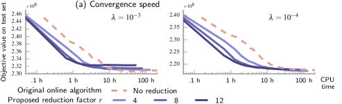
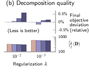
Figure 1: Acceleration of sparse matrix factorization with random subsampling on the HCP dataset (2TB). Reducing streamed data with stochastic masks permits $10\times$ speed-ups without deteriorating goodness of fit on test data nor alterating sparsity of final dictionary.

Relation to classical matrix completion formulation.

Our model is related to the classical $\ell_{2}$-penalized matrix completion model (e.g. Bell & Koren, 2007) we rewrite

$$\sum_{i=1}^{n}\|{\mathbf{M}}_{i}({\mathbf{x}}_{i}-{\mathbf{D}}^{\top}\boldsymbol{\alpha}_{i}\!)\|_{2}^{2}+\lambda s_{i}\|\boldsymbol{\alpha}_{i}\|_{2}^{2}+\lambda\|(\sum_{i=1}^{n}{\mathbf{M}}_{i})^{\frac{1}{2}}{\mathbf{D}}\|_{2}^{2}$$ (23)

With quadratic regularization on ${\mathbf{D}}$ and ${\mathbf{A}}$ – that is, using $\Omega=\|.\|_{2}^{2}$ and $\psi=\|.\|_{2}$ – (11) only differs in that it uses a penalization on ${\mathbf{D}}$ instead of a constraint. Srebro et al. (2004) introduced the trace-norm regularization to solve a convex problem equivalent to (23). The major difference is that we adopt a non-convex optimization strategy, thus losing the benefits of convexity, but gaining on the other hand the possibility of using stochastic optimization.

Practical considerations.

Our algorithm can be slightly modified to use weights $w_{t}$ that differ from $\frac{1}{t}$ for ${\mathbf{B}}$ and ${\mathbf{C}}$, as advocated by Mairal (2013). It also proves beneficial to perform code computation on mini-batches of masked samples. Update of the dictionary is performed on the rows that are seen at least once in the masks $({\mathbf{M}}_{t})_{\textrm{batch}}$.

3 Experiments

The proposed algorithm was designed to handle massive datasets: masking data enables streaming a sequence $({\mathbf{M}}_{t}{\mathbf{x}}_{t})_{t}$ instead of $({\mathbf{x}}_{t})_{t}$, reducing single-iteration computational complexity and IO stress of a factor $r=\frac{p}{{\mathbb{E}}({\mathrm{Tr}\;}{\mathbf{M}})}$, while accessing an accurate description of the data. Hence, we analyze in detail how our algorithm improves performance for sparse decomposition of fMRI datasets. Moreover, as it relies on data masks, our algorithm is well suited for matrix completion, to reconstruct a data stream $({\mathbf{x}}_{t})_{t}$ from the masked stream $({\mathbf{M}}_{t}{\mathbf{x}}_{t})_{t}$. We demonstrate the accuracy of our algorithm on explicit recommender systems and show considerable computational speed-ups compared to an efficient coordinate-descent based algorithm.

We use scikit-learn (Pedregosa et al., 2011) in experiments, and have released a python package for reproducibility.

3.1 Sparse Matrix Factorization for fMRI

Context.

Matrix factorization has long been used on functional Magnetic Resonance Imaging (McKeown et al., 1998). Data are temporal series of 3D images of brain activity, to decompose in spatial modes capturing regions that activate together. The matrices to decompose are dense and heavily redundant, both spatially and temporally: close voxels and successive records are correlated. Data can be huge: we use the whole HCP dataset (Van Essen et al., 2013), with $n=2.4\cdot 10^{6}$ (2000 records, 1 200 time points) and $p=2\cdot 10^{5}$, totaling 2 TB of dense data.

Interesting dictionaries for neuroimaging capture spatially-localized components, with a few brain regions. This can be obtained by enforcing sparsity on the dictionary: in our formalism, this is achieved with $\ell_{1}$-ball projection for ${\mathbf{D}}$. We set $\mathcal{C}=\mathcal{B}_{1}^{k}$, and $\Omega=\|\cdot\|_{2}^{2}$. Historically, such decomposition have been obtained with the classical dictionary learning objective on transposed data (Varoquaux et al., 2013): the code ${\mathbf{A}}$ holds sparse spatial maps and voxel time-series are streamed. However, given the size of $n$ for our dataset, this method is not usable in practice.

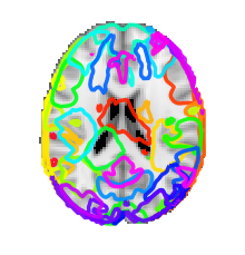
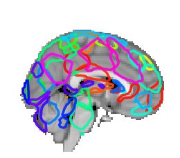
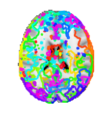
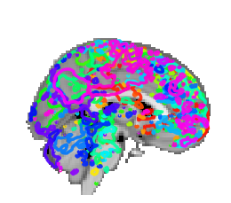
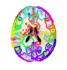
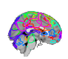
235 h run time                    Original online algorithm                            1 full epoch                         10 h run time                    Original online algorithm                            $\frac{1}{24}$ epoch                         10 h run time                    Proposed algorithm                            $\frac{1}{2}$ epoch, reduction $r{=}12$                         

Figure 2: Brain atlases: outlines of each map at half the maximum value ($\lambda=10^{-4}$). Left: the reference algorithm on the full dataset. Middle: the reference algorithm on a twentieth of the dataset. Right: the proposed algorithm with a similar run time: half the dataset and $r=9$. Compared to a full run of the baseline algorithm, the figure explore two possible strategies to decrease computation time: processing less data (middle), or our approach (right). Our approach achieves a result closer to the gold standard in a given time budget.

Handling such volume of data sets new constraints. First, efficient disk access becomes critical for speed. In our case, learning the dictionary is done by accessing the data in row batches, which is coherent with fMRI data storage: no time is lost seeking data on disk. Second, reducing IO load on the storage is also crucial, as it lifts bottlenecks that appear when many processes access the same storage at the same time, e.g. during cross-validation on $\lambda$ within a supervised pipeline. Our approach reduces disk usage by a factor $r$. Finally, parallel methods based on message passing, such as asynchronous coordinate descent, are unlikely to be efficient given the network / disk bandwidth that each process requires to load data. This makes it crucial to design efficient sequential algorithms.

Experiment

We quantify the effect of random subsampling for sparse matrix factorization, in term of speed and accuracy. A natural performance evaluation is to measure an empirical estimate of the loss $l$ defined in Eq. 4 from unseen data, to rule out any overfitting effect. For this, we evaluate $l$ on a test set $({\mathbf{x}}_{i})_{i<N}$. Pratically, we sample $({\mathbf{x}}_{t})_{t}$ in a pseudo-random manner: we randomly select a record, from where we select a random batch of rows ${\mathbf{x}}_{t}$ – we use a batch size of $40$, empirically found to be efficient. We load ${\mathbf{M}}_{t}{\mathbf{x}}_{t}$ in memory and perform an iteration of the algorithm. The mask sequence is sampled by breaking random permutation vectors into chunks of size $p/r$.

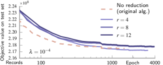
Figure 3: Evolution of objective function with epochs for three reduction factors. Learning speed per epoch is little reduced by stochastic subsampling, despite the speed-up factor it provides.

Results

Fig. 1(a) compares our algorithm with subsampling ratios $r$ in $\{4,8,12\}$ to vanilla online dictionary learning algorithm $(r=1)$, plotting trajectories of the test objective against real CPU time. There is no obvious choice of $\lambda$ due to the unsupervised nature of the problem: we use $10^{-3}$ and $10^{-4}$, that bounds the range of $\lambda$ providing interpretable dictionaries.

First, we observe the convergence of the objective function for all tested $r$, providing evidence that the approximations made in the derivation of update rules does not break convergence for such $r$. Fig. 1(b) shows the validity of the obtained dictionary relative to the reference output: both objective function and $\ell_{1}{/}\ell_{2}$ ratio – the relevant value to measure sparsity in our setting – are comparable to the baseline values, up to $r=8$. For high regularization and $r=12$, our algorithm tends to yield somewhat sparser solutions ($5\%$ lower $\ell_{1}{/}\ell_{2}$) than the original algorithm, due to the approximate $\ell_{1}$-projection we perform. Obtained maps still proves as interpretable as with baseline algorithm.

Our algorithm proves much faster than the original one in finding a good dictionary. Single iteration time is indeed reduced by a factor $r$, which enables our algorithm to go over a single epoch $r$ times faster than the vanilla algorithm and capture the variability of the dataset earlier. To quantify speed-ups, we plot the empirical objective value of ${\mathbf{D}}$ against the number of observed records in Fig. 3. For $r\leq 12$, increasing $r$ little reduces convergence speed per epoch: random subsampling does not shrink much the quantity of information learned at each iteration.

This brings a near $\times r$ speed-up factor: for high and low regularization respectively, our algorithm converges in $3$ and $10$ hours with subsampling factor $r=12$, whereas the vanilla online algorithm requires about $30$ and $100$ hours. Qualitatively, Fig. 2 shows that with the same time budget, the proposed reduction approach with $r=12$ on half of the data gives better results than processing a small fraction of the data without reduction: segmented regions are less noisy and closer to processing the full data.

These results advocates the use of a subsampling rate of $r\approx 10$ in this setting. When sparse matrix decomposition is part of a supervised pipeline with scoring capabilities, it is possible to find $r$ efficiently: start by setting it dereasonably high and decrease it geometrically until supervised performance (e.g. in classification) ceases to improve.

3.2 Collaborative Filtering with Missing Data

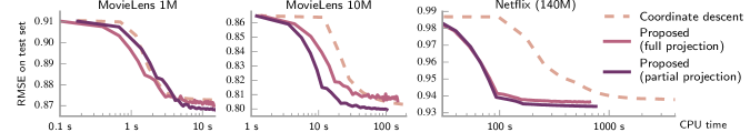
Figure 4: Learning speed for collaborative filtering for datasets of different size: the larger the dataset, the greater our speed-up.

We validate the performance of the proposed algorithm on recommender systems for explicit feedback, a well-studied matrix completion problem. We evaluate the scalability of our method on datasets of different dimension: MovieLens 1M, MovieLens 10M, and 140M ratings Netflix dataset.

We compare our algorithm to a coordinate-descent based method (Yu et al., 2012), that provides state-of-the art convergence time performance on our largest dataset. Although stochastic gradient descent methods for matrix factorization can provide slightly better single-run performance (Takács et al., 2009), these are notoriously hard to tune and require a precise grid search to uncover a working schedule of learning rates. In contrast, coordinate descent methods do not require any hyper-parameter setting and are therefore more efficient in practice. We benchmarked various recommender-system codes (MyMediaLite, LibFM, SoftImpute, spira), and chose coordinate descent algorithm from spira as it was by far the fastest.

Completion from dictionary ${\mathbf{D}}_{t}$.

We stream user ratings to our algorithm: $p$ is the number of movies and $n$ is the number of users. As $n\gg p$ on Netflix dataset, this increases the benefit of using an online method. We have observed comparable prediction performance streaming item ratings. Past the first epoch, at iteration $t$, every column $i$ of ${\mathbf{X}}$ can be predicted by the last code $\boldsymbol{\alpha}_{l(i,t)}$ that was computed from this column at iteration $l(i,t)$. At iteration $t$, for all $i<[n]$, ${\mathbf{x}}_{i}^{\textrm{pred}}={\mathbf{D}}\boldsymbol{\alpha}_{l(i,t)}$. Prediction thus only requires an additional matrix computation after the factorization.

Preprocessing.

Successful prediction should take into account user and item biases. We compute these biases on train data following Hastie et al. (2014) (alternated debiasing). We use them to center the samples $({\mathbf{x}}_{t})_{t}$ that are streamed to the algorithm, and to perform final prediction.

Tools and experiments.

Both baseline and proposed algorithm are implemented in a computationally optimal way, enabling fair comparison based on CPU time. Benchmarks were run using a single 2.7 GHz Xeon CPU, with a 30 components dictionary. For Movielens datasets, we use a random $25\%$ of data for test and the rest for training. We average results on five train/test split for MovieLens in Table 1. On Netflix, the probe dataset is used for testing. Regularization parameter $\lambda$ is set by cross-validation on the training set: the training data is split 3 times, keeping $33\%$ of Movielens datasets for evaluation and $1\%$ for Netflix, and grid search is performed on 15 values of $\lambda$ between $10^{-2}$ and $10$. We assess the quality of obtained decomposition by measuring the root mean square error (RMSE) between prediction on the test set and ground truth. We use mini-batches of size $\frac{n}{100}$.

Table 1: Comparison of performance and convergence time for online masked matrix factorization and coordinate descent method. Convergence time: score is under 0.1% deviation from final root mean squared error on test set – 5 runs average. CD: coordinate descent; MODL: masked online dictionary learning.

Dataset	Test RMSE		Convergence time		Speed
	CD	MODL	CD	MODL	-up
ML 1M	$0.872$	$\mathbf{0.866}$	$\mathbf{6\,s}$	$8\,s$	$\times 0.75$
ML 10M	$0.802$	$\mathbf{0.799}$	$223\,s$	$\mathbf{60\,s}$	$\times 3.7$
NF (140M)	$0.938$	$\mathbf{0.934}$	$1714\,s$	$\mathbf{256\,s}$	$\times 6.8$

Results.

We report the evolution of test RMSE along time in Fig. 4, along with its value at convergence and numerical convergence time in Table 1. Benchmarks are performed on the final run, after selection of parameter $\lambda$.

The two variants of the proposed method converge toward a solution that is at least as good as that of coordinate descent, and slightly better on Movielens 10M and Netflix. Our algorithm brings a substantial performance improvement on medium and large scale datasets. On Netflix, convergence is almost reached in $4$ minutes (score under $0.1\%$ deviation from final RMSE), which makes our method $6.8$ times faster than coordinate descent. Moreover, the relative performance of our algorithm increases with dataset size. Indeed, as datasets grow, less epochs are needed for our algorithm to reach convergence (Fig. 4). This is a significant advantage over coordinate descent, that requires a stable number of cycle on coordinates to reach convergence, regardless of dataset size. The algorithm with partial projection performs slightly better. This can be explained by the extra regularization on $({\mathbf{D}}_{t})_{t}$ brought by this heuristic.

Learning weights.

Unlike SGD, and similar to the vanilla online dictionary learning algorithm, our method does not critically suffer from hyper-parameter tuning. We tried weights $w_{t}=\frac{1}{t^{\beta}}$ as described in Sec. 2.3, and observed that a range of $\beta$ yields fast convergence. Theoretically, Mairal (2013) shows that stochastic majorization-minimization converges when $\beta~{}\in~{}(.75,1]$. We verify this empirically, and obtain optimal convergence speed for $\beta\in[.85,0.95]$. (Fig. 5). We report results for $\beta=0.9$.

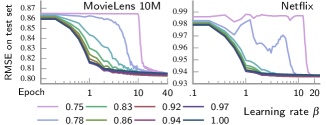
Figure 5: Learning weights: on two different datasets, optimal convergence is obtained for $\beta\in[.85,\;.95]$, predicted by theory.

4 Conclusion

Whether it is sensor data, as fMRI, or e-commerce databases, sample sizes and number of features are rapidly growing, rendering current matrix factorization approaches intractable. We have introduced a online algorithm that leverages random feature subsampling, giving up to 8-fold speed and memory gains on large data. Datasets are getting bigger, and they often come with more redundancies. Such approaches blending online and randomized methods will yield even larger speed-ups on next-generation data.

References

- Aharon et al. (2006) Aharon, Michal, Elad, Michael, and Bruckstein, Alfred. k-SVD: An algorithm for designing overcomplete dictionaries for sparse representation. IEEE Transactions on Signal Processing, 54(11):4311–4322, 2006.
- Bell & Koren (2007) Bell, Robert M. and Koren, Yehuda. Lessons from the Netflix prize challenge. ACM SIGKDD Explorations Newsletter, 9(2):75–79, 2007.
- Bingham & Mannila (2001) Bingham, Ella and Mannila, Heikki. Random projection in dimensionality reduction: applications to image and text data. In Proceedings of ACM SIGKDD International Conference on Knowledge Discovery and Data Mining, pp. 245–250. ACM, 2001.
- Blondel et al. (2015) Blondel, Mathieu, Fujino, Akinori, and Ueda, Naonori. Convex factorization machines. In Machine Learning and Knowledge Discovery in Databases, pp. 19–35. Springer, 2015.
- Bottou (2010) Bottou, Léon. Large-scale machine learning with stochastic gradient descent. In Proceedings of COMPSTAT, pp. 177–186. Springer, 2010.
- Candès & Recht (2009) Candès, Emmanuel J. and Recht, Benjamin. Exact matrix completion via convex optimization. Foundations of Computational Mathematics, 9(6):717–772, 2009.
- Candès & Tao (2006) Candès, Emmanuel J. and Tao, Terence. Near-optimal signal recovery from random projections: Universal encoding strategies? Information Theory, IEEE Transactions on, 52(12):5406–5425, 2006.
- Duchi et al. (2008) Duchi, John, Shalev-Shwartz, Shai, Singer, Yoram, and Chandra, Tushar. Efficient projections onto the l 1-ball for learning in high dimensions. In Proceedings of the International Conference on Machine Learning, pp. 272–279. ACM, 2008.
- Halko et al. (2009) Halko, Nathan, Martinsson, Per-Gunnar, and Tropp, Joel A. Finding structure with randomness: Probabilistic algorithms for constructing approximate matrix decompositions. arXiv:0909.4061 [math], 2009.
- Hastie et al. (2014) Hastie, Trevor, Mazumder, Rahul, Lee, Jason, and Zadeh, Reza. Matrix completion and low-rank SVD via fast alternating least squares. arXiv:1410.2596 [stat], 2014.
- Johnson & Lindenstrauss (1984) Johnson, William B. and Lindenstrauss, Joram. Extensions of Lipschitz mappings into a Hilbert space. Contemporary mathematics, 26(189-206):1, 1984.
- Mairal (2013) Mairal, Julien. Stochastic majorization-minimization algorithms for large-scale optimization. In Advances in Neural Information Processing Systems, pp. 2283–2291, 2013.
- Mairal (2014) Mairal, Julien. Sparse Modeling for Image and Vision Processing. Foundations and Trends in Computer Graphics and Vision, 8(2-3):85–283, 2014.
- Mairal et al. (2010) Mairal, Julien, Bach, Francis, Ponce, Jean, and Sapiro, Guillermo. Online learning for matrix factorization and sparse coding. The Journal of Machine Learning Research, 11:19–60, 2010.
- McKeown et al. (1998) McKeown, M. J., Makeig, S., Brown, G. G., Jung, T. P., Kindermann, S. S., Bell, A. J., and Sejnowski, T. J. Analysis of fMRI Data by Blind Separation into Independent Spatial Components. Human Brain Mapping, 6(3):160–188, 1998. ISSN 1065-9471.
- Pedregosa et al. (2011) Pedregosa, Fabian, Varoquaux, Gaël, Gramfort, Alexandre, Michel, Vincent, Thirion, Bertrand, Grisel, Olivier, Blondel, Mathieu, Prettenhofer, Peter, Weiss, Ron, Dubourg, Vincent, Vanderplas, Jake, Passos, Alexandre, Cournapeau, David, Brucher, Matthieu, Perrot, Matthieu, and Duchesnay, Édouard. Scikit-learn: machine learning in Python. Journal of Machine Learning Research, 12:2825–2830, 2011.
- Pourkamali-Anaraki et al. (2015) Pourkamali-Anaraki, Farhad, Becker, Stephen, and Hughes, Shannon M. Efficient dictionary learning via very sparse random projections. In Proceedings of the IEEE International Conference on Sampling Theory and Applications, pp. 478–482. IEEE, 2015.
- Rendle (2010) Rendle, Steffen. Factorization machines. In Proceedings of the IEEE International Conference on Data Mining, pp. 995–1000. IEEE, 2010.
- Rendle & Schmidt-Thieme (2008) Rendle, Steffen and Schmidt-Thieme, Lars. Online-updating regularized kernel matrix factorization models for large-scale recommender systems. In Proceedings of the ACM Conference on Recommender systems, pp. 251–258. ACM, 2008.
- Srebro et al. (2004) Srebro, Nathan, Rennie, Jason, and Jaakkola, Tommi S. Maximum-margin matrix factorization. In Advances in Neural Information Processing Systems, pp. 1329–1336, 2004.
- Szabó et al. (2011) Szabó, Zoltán, Póczos, Barnabás, and Lorincz, András. Online group-structured dictionary learning. In Proceedings of the IEEE Conference on Computer Vision and Pattern Recognition, pp. 2865–2872. IEEE, 2011.
- Takács et al. (2009) Takács, Gábor, Pilászy, István, Németh, Bottyán, and Tikk, Domonkos. Scalable collaborative filtering approaches for large recommender systems. The Journal of Machine Learning Research, 10:623–656, 2009.
- Van Essen et al. (2013) Van Essen, David C., Smith, Stephen M., Barch, Deanna M., Behrens, Timothy E. J., Yacoub, Essa, and Ugurbil, Kamil. The WU-Minn Human Connectome Project: An overview. NeuroImage, 80:62–79, 2013.
- Varoquaux et al. (2011) Varoquaux, Gaël, Gramfort, Alexandre, Pedregosa, Fabian, Michel, Vincent, and Thirion, Bertrand. Multi-subject dictionary learning to segment an atlas of brain spontaneous activity. In Proceedings of the Information Processing in Medical Imaging Conference, volume 22, pp. 562–573. Springer, 2011.
- Varoquaux et al. (2013) Varoquaux, Gaël, Schwartz, Yannick, Pinel, Philippe, and Thirion, Bertrand. Cohort-level brain mapping: learning cognitive atoms to single out specialized regions. In Proceedings of the Information Processing in Medical Imaging Conference, pp. 438–449. Springer, 2013.
- Yu et al. (2012) Yu, Hsiang-Fu, Hsieh, Cho-Jui, and Dhillon, Inderjit. Scalable coordinate descent approaches to parallel matrix factorization for recommender systems. In Proceedings of the International Conference on Data Mining, pp. 765–774. IEEE, 2012.