The entanglement negativity in random spin chains

Paola Ruggiero International School for Advanced Studies (SISSA), Via Bonomea 265, 34136, Trieste, Italy, INFN, Sezione di Trieste    Vincenzo Alba International School for Advanced Studies (SISSA), Via Bonomea 265, 34136, Trieste, Italy, INFN, Sezione di Trieste    Pasquale Calabrese International School for Advanced Studies (SISSA), Via Bonomea 265, 34136, Trieste, Italy, INFN, Sezione di Trieste
Abstract

We investigate the logarithmic negativity in strongly-disordered spin chains in the random-singlet phase. We focus on the spin-1/2121/2 random Heisenberg chain and the random XX𝑋𝑋XX chain. We find that for two arbitrary intervals the disorder-averaged negativity and the mutual information are proportional to the number of singlets shared between the two intervals. Using the strong-disorder renormalization group (SDRG), we prove that the negativity of two adjacent intervals grows logarithmically with the intervals length. In particular, the scaling behavior is the same as in conformal field theory, but with a different prefactor. For two disjoint intervals the negativity is given by a universal simple function of the cross ratio, reflecting scale invariance. As a function of the distance of the two intervals, the negativity decays algebraically in contrast with the exponential behavior in clean models. We confirm our predictions using a numerical implementation of the SDRG method. Finally, we also implement DMRG simulations for the negativity in open spin chains. The chains accessible in the presence of strong disorder are not sufficiently long to provide a reliable confirmation of the SDRG results.

I Introduction

Entanglement measures are nowadays accepted as powerful tools to characterize quantum many-body systems amico-2008 ; calabrese-2009 ; eisert-2010 ; laflorencie-2016 . Arguably, the most popular and useful one is the entanglement entropy. Given a pure state |ψket𝜓|\psi\rangle and a bipartition into two parts A𝐴A and B𝐵B, the entanglement entropy of part A𝐴A is defined as

SATrρAlnρA,subscript𝑆𝐴Trsubscript𝜌𝐴subscript𝜌𝐴S_{A}\equiv-\textrm{Tr}\rho_{A}\ln\rho_{A}, (1)

where ρATrB|ψψ|subscript𝜌𝐴subscriptTr𝐵ket𝜓bra𝜓\rho_{A}\equiv\textrm{Tr}_{B}|\psi\rangle\langle\psi| is the reduced density matrix of A𝐴A. For a pure state it is clear that SA=SBsubscript𝑆𝐴subscript𝑆𝐵S_{A}=S_{B}, reflecting the property that a good measure of entanglement is symmetric in A𝐴A and B𝐵B.

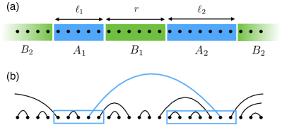
If a system is in a mixed state, for instance at finite temperature, a useful measure of the correlation between A𝐴A and B𝐵B is the mutual information A:Bsubscript:𝐴𝐵{\mathcal{I}}_{A:B}, which is defined as the symmetrized combination A:BSA+SBSABsubscript:𝐴𝐵subscript𝑆𝐴subscript𝑆𝐵subscript𝑆𝐴𝐵{\mathcal{I}}_{A:B}\equiv S_{A}+S_{B}-S_{A\cup B}. However, it is well known that the mutual information provides only an upper bound for the entanglement between A𝐴A and B𝐵B, as it is sensitive to both classical and quantum correlations. A similar issue arises when quantifying the entanglement between disconnected regions in pure states. For instance, given the tripartition of a system as B2A1B1A2B2subscript𝐵2subscript𝐴1subscript𝐵1subscript𝐴2subscript𝐵2B_{2}\cup A_{1}\cup B_{1}\cup A_{2}\cup B_{2} (as illustrated in Fig. 1 (a) for a spin chain), with AA1A2𝐴subscript𝐴1subscript𝐴2A\equiv A_{1}\cup A_{2} the region of interest, A1:A2subscript:subscript𝐴1subscript𝐴2{\mathcal{I}}_{A_{1}:A_{2}} is not a measure of the mutual entanglement between A1subscript𝐴1A_{1} and A2subscript𝐴2A_{2}.

A computable measure of the mutual entanglement between two subsystems in a mixed state is provided by the so-called logarithmic negativity peres-1996 ; zycz-1998 ; zycz-1999 ; lee-2000 ; vidal-2002 ; plenio-2005

lnρAT21=lnTr|ρAT2|.subscriptnormsuperscriptsubscript𝜌𝐴subscript𝑇21Trsubscriptsuperscript𝜌subscript𝑇2𝐴{\cal E}\equiv\ln||\rho_{A}^{T_{2}}||_{1}=\ln\textrm{Tr}|\rho^{T_{2}}_{A}|. (2)

Here ρAT2superscriptsubscript𝜌𝐴subscript𝑇2\rho_{A}^{T_{2}} is the partially transposed reduced density matrix with respect to A2subscript𝐴2A_{2}. This is defined as φ1φ2|ρAT2|φ1φ2φ1φ2|ρA|φ1φ2quantum-operator-productsubscript𝜑1subscript𝜑2subscriptsuperscript𝜌subscript𝑇2𝐴subscriptsuperscript𝜑1subscriptsuperscript𝜑2quantum-operator-productsubscript𝜑1superscriptsubscript𝜑2subscript𝜌𝐴subscriptsuperscript𝜑1subscript𝜑2\langle\varphi_{1}\varphi_{2}|\rho^{T_{2}}_{A}|\varphi^{\prime}_{1}\varphi^{\prime}_{2}\rangle\equiv\langle\varphi_{1}\varphi_{2}^{\prime}|\rho_{A}|\varphi^{\prime}_{1}\varphi_{2}\rangle, with {φ1}subscript𝜑1\{\varphi_{1}\} and {φ2}subscript𝜑2\{\varphi_{2}\} being bases for A1subscript𝐴1A_{1} and A2subscript𝐴2A_{2}, respectively.

Refer to caption
Figure 1: (a): Partition of an infinite spin chain corresponding to two disjoint intervals. The region of interest is A1A2subscript𝐴1subscript𝐴2A_{1}\cup A_{2}. Two adjacent intervals correspond to r=0𝑟0r=0. (b): Cartoon of the random singlet phase. The lines connect pairs of spins forming SU(2)𝑆𝑈2SU(2) singlets. The entanglement negativity A1:A2subscript:subscript𝐴1subscript𝐴2{\cal E}_{A_{1}:A_{2}} is proportional to the number of singlets nA1:A2subscript𝑛:subscript𝐴1subscript𝐴2n_{A_{1}:A_{2}} shared between A1subscript𝐴1A_{1} and A2subscript𝐴2A_{2} (here nA1:A2=1subscript𝑛:subscript𝐴1subscript𝐴21n_{A_{1}:A_{2}}=1).

Besides its interest in quantum information, recently the negativity became the focus of several interdisciplinary efforts to understand its role in many-body systems. For critical points described by a Conformal Field Theory (CFT) its scaling behavior has been derived analytically calabrese-2012 ; cct-neg-long ; calabrese-2013 . This allowed to prove that, unlike the entanglement entropy, the negativity is scale invariant in gapless systems described by CFT, as it was already argued based on DMRG white-1992 ; uli1 ; uli2 simulations hannu-2008 , on semi-analytic results for the harmonic chain mrpr-09 , and for mean-field exactly solvable spin models hannu-2010 . Furthermore, for disjoint intervals the logarithmic negativity contains, in principle, complete information about the intricate structure of the underlying CFT calabrese-2012 (as it does the entanglement entropy of two or more disjoint intervals 2int ). Some of these results have been generalized to finite-temperature calabrese-2015 , large central charge kpp-14 , out of equilibrium situations ctc-14 ; hoogeveen-2015 ; eisler-2014 ; wen-2015 , and holographicrr-15 and massive quantum field theories fournier-2015 . In topologically ordered phases, i.e., characterized by a non-zero topological entropy levin-2006 ; kitaev-2006 , it has been shown that the negativity is sensitive only to the “quantum” contribution lee-2013 ; castelnovo-2013 , while it is zero in classical topologically ordered states. Also, the negativity proved to be a useful tool to characterize Kondo-like behavior in spin chains bayat-2012 ; bayat-2014 ; abab-16 . Surprisingly, the exact treatment of the partial transposition in free fermion models is an arduous task, and no exact results are known yet for the negativity, despite some recent progresses for the calculations of the moments of the partial transpose eisler-2014 ; coser-2015 ; ctc-16 ; ctc-16b ; chang-2016 ; hw-16 . Oppositely, the negativity can be calculated analytically for free bosonic models audenaert-2002 . for which few results are also available in higher dimensions eisler-2016 ; dct-16 . Furthermore, some interesting results on the negativity in Chern-Simons theories have been provided recently wen-2016 . Finally, from the numerical perspective, effective methods to calculate the negativity are available in the context of Tree Tensor Networks calabrese-2013 , while the moments of the partially transposed reduced density matrix can be calculated using classical alba-2013 and quantum chung-2014 Monte Carlo techniques. When not analytically possible, numerical extrapolations can be used to obtain the negativity from the replica limit of the moments dct-15 .

At the same time the study of the interplay between disorder and entanglement became a fruitful research area refael-2009 ; laflorencie-2016 . For instance, in Ref. RefaelMoore2004, it has been shown that, for disordered spin chains exhibiting the random singlet (RS) phase, the scaling of the disorder averaged entanglement entropy is logarithmic with the subsystem size like in a CFT. This has been tested numerically in the random XX𝑋𝑋XX chainlaflorencie-2005 (which is exactly solvable for each realization of the disorder), and in the random XXX𝑋𝑋𝑋XXX chain dechiara-2006 using DMRG. Furthermore, the moments of the reduced density matrix TrρAαTrsuperscriptsubscript𝜌𝐴𝛼\textrm{Tr}\rho_{A}^{\alpha} have been also studied FagottiCalabreseMoore2011 , as well as the spectrum py-13 , and the entanglement in low-lying excited states ramirez-2014 . Other disordered spin models raul-2006 ; refael-2007 ; hvlm-07 ; lir-07 ; by-07 ; bcmr-07 ; il-08 ; frbm-08 ; ysh-08 ; hlvv-11 ; ki-12 ; gah-16 ; rsrs-16 have been also considered, obtaining similar results for the scaling of the entanglement entropy. The non-equilibrium features of the entanglement in these random spin chains are also under intensive investigation dechiara-2006 ; bo-07 ; isl-12 ; bpm-12 ; spa-13 ; va-14 ; prado-14 ; vm-15 ; zas-16 . The behavior of entanglement related quantities in classical disordered spin systems has been explored alba-2016 .

In this paper we investigate the disorder averaged logarithmic negativity in RS phases in the framework of the strong-disorder renormalization group (SDRG) Igloi-rev . We focus on the spin-1/2121/2 Heisenberg (XXX𝑋𝑋𝑋XXX) chain with random antiferromagnetic couplings, and on the random XX𝑋𝑋XX chain. We consider both adjacent and disjoint intervals (see Fig. 1 (a)). We demonstrate that in a RS phase the negativity of two intervals is always proportional to the number of singlets shared between them. Surprisingly, due to the simple structure of the RS phase, this is also the case for the mutual information, which is given as A1:A2=2A1:A2subscript:subscript𝐴1subscript𝐴22subscript:subscript𝐴1subscript𝐴2{\mathcal{I}}_{A_{1}:A_{2}}=2{\cal E}_{A_{1}:A_{2}}. More quantitatively, we find that for two adjacent intervals embedded in an infinite chain the disorder-averaged negativity scales as

A1:A2=ln26ln(121+2)+k,subscript:subscript𝐴1subscript𝐴226subscript1subscript2subscript1subscript2𝑘{\cal E}_{A_{1}:A_{2}}=\frac{\ln 2}{6}\ln\Big{(}\frac{\ell_{1}\ell_{2}}{\ell_{1}+\ell_{2}}\Big{)}+k, (3)

for large 1subscript1\ell_{1} and 2subscript2\ell_{2} (the lengths of the two intervals). Here k𝑘k is an additive constant. Interestingly, Eq. (3) has the same functional dependence on 1,2subscript12\ell_{1,2} as in CFT calabrese-2012 , but the prefactor of the logarithm is different. For two disjoint intervals (see Fig. 1 (a)), we obtain

A1:A2=ln26ln(1+r)(2+r)r(1+2+r)=ln26ln(1x).subscript:subscript𝐴1subscript𝐴226subscript1𝑟subscript2𝑟𝑟subscript1subscript2𝑟261𝑥{\cal E}_{A_{1}:A_{2}}=\frac{\ln 2}{6}\ln\frac{(\ell_{1}+r)(\ell_{2}+r)}{r(\ell_{1}+\ell_{2}+r)}=-\frac{\ln 2}{6}\ln(1-x). (4)

Here 1,2subscript1subscript2\ell_{1},\ell_{2} are the intervals length, and r𝑟r their distance. Eq. (4) is scale invariant and for this reason the r.h.s. has been written as a function of the cross ratio

x=12(1+r)(1+r).𝑥subscript1subscript2subscript1𝑟subscript1𝑟x=\frac{\ell_{1}\ell_{2}}{(\ell_{1}+r)(\ell_{1}+r)}. (5)

Again, this is similar to the CFT case, where A1:A2subscript:subscript𝐴1subscript𝐴2{\cal E}_{A_{1}:A_{2}} depends in a more intricate way on x𝑥x calabrese-2012 ; cct-neg-long . Interestingly, in the limit of two intervals far apart, from (4) one has the power-law decay r2proportional-tosuperscript𝑟2{\cal E}\propto r^{-2}, in contrast with the CFT case, where this decay is exponential calabrese-2012 . Both (3) and (4) turn out to be in perfect agreement with exact results obtained from a numerical implementation of the SDRG for the random XXX𝑋𝑋𝑋XXX chain.

Finally, by generalizing the method of Ref. hannu-2008, , we discuss how to obtain the logarithmic negativity in DMRG simulations itensor for arbitrary tripartitions of the spin chain. The computational cost of the algorithm is χmax6proportional-toabsentsubscriptsuperscript𝜒6𝑚𝑎𝑥\propto\chi^{6}_{max}, with χmaxsubscript𝜒𝑚𝑎𝑥\chi_{max} the maximal bond dimension of the matrix product state (MPS). As a byproduct of our analysis we numerically verify the CFT scaling of the negativity of two adjacent intervals in the clean XX𝑋𝑋XX chain. In the presence of randomness it is numerically challenging to ensure the convergence of DMRG, introducing a systematic error in the numerical data. The latter is negligible only for small chains and weak disorder. The accessible chain sizes are not sufficient to provide reliable numerical evidence for (3) and (4).

The manuscript is organized as follows. In section II we introduce the XXZ𝑋𝑋𝑍XXZ spin-1/2121/2 chain with random antiferromagnetic couplings and summarize the strong disorder renormalization group (SDRG) method. In section III we provide the analytic expressions for the logarithmic negativity and the moments of the partially transposed reduced density matrix in RS phases. The scaling of the negativity is discussed in section IV for both adjacent and disjoint intervals. These results are verified in section V using a numerical implemtation of the SDRG method. Section VI focuses on the calculation of the logarithmic negativity in DMRG simulations. In section VII we present DMRG results for the negativity of two adjacent intervals in the random XX𝑋𝑋XX chain. Finally, we conclude in section VIII.

II The disordered Heisenberg spin chain and the strong disorder RG

The random antiferromagnetic spin-1212\frac{1}{2} XXZ𝑋𝑋𝑍XXZ chain with open boundary conditions (OBC) is defined by the Hamiltonian

=i=1L1Ji(SixSi+1x+SiySi+1y+ΔSizSi+1z),superscriptsubscript𝑖1𝐿1subscript𝐽𝑖subscriptsuperscript𝑆𝑥𝑖subscriptsuperscript𝑆𝑥𝑖1subscriptsuperscript𝑆𝑦𝑖subscriptsuperscript𝑆𝑦𝑖1Δsubscriptsuperscript𝑆𝑧𝑖subscriptsuperscript𝑆𝑧𝑖1{\mathcal{H}}=\sum\limits_{i=1}^{L-1}J_{i}(S^{x}_{i}S^{x}_{i+1}+S^{y}_{i}S^{y}_{i+1}+\Delta S^{z}_{i}S^{z}_{i+1}), (6)

where Six,y,zsuperscriptsubscript𝑆𝑖𝑥𝑦𝑧S_{i}^{x,y,z} are the spin components acting on site i𝑖i, L𝐿L is the length of the chain, ΔΔ\Delta the anisotropy parameter, and {Ji}i=1L1superscriptsubscriptsubscript𝐽𝑖𝑖1𝐿1\{J_{i}\}_{i=1}^{L-1} are uncorrelated positive random variables, drawn from a distribution P(J)𝑃𝐽P(J). For periodic boundary conditions (PBC) one has an extra term in (6) connecting site L𝐿L with site 111. We focus on Δ=1Δ1\Delta=1 and Δ=0Δ0\Delta=0, corresponding to the XXX𝑋𝑋𝑋XXX and the XX𝑋𝑋XX random chain, respectively. For generic {Ji}i=1L1superscriptsubscriptsubscript𝐽𝑖𝑖1𝐿1\{J_{i}\}_{i=1}^{L-1}, the latter can be treated analytically for each realization of the disorder, exploiting the mapping to free fermions (see Appendix A). Here we restrict ourselves to the family of distributions

Pδ(J)δ1J1+1/δ,subscript𝑃𝛿𝐽superscript𝛿1superscript𝐽11𝛿P_{\delta}(J)\equiv\delta^{-1}J^{-1+1/\delta}, (7)

with J[0,1]𝐽01J\in[0,1], and 0δ<0𝛿0\leq\delta<\infty a parameter tuning the disorder strength. For δ0𝛿0\delta\to 0 one recovers the clean, i.e., without disorder, XXZ𝑋𝑋𝑍XXZ chain, whereas δ𝛿\delta\to\infty corresponds to the infinite-randomness fixed point (IRFP, see section II). The latter describes the low-energy physics of (6), irrespective of the chosen distribution P(J)𝑃𝐽P(J). For δ=1𝛿1\delta=1, Pδ(J)subscript𝑃𝛿𝐽P_{\delta}(J) becomes the flat distribution (box distribution) in the interval [0,1]01[0,1].

We now briefly review the SDRG method for the XXX𝑋𝑋𝑋XXX chain. The main idea is to obtain a low-energy effective description of (6) by successively integrating out the strongest couplings, and renormalizing the remaining ones. Given an arbitrary coupling configuration {Ji}i=1L1superscriptsubscriptsubscript𝐽𝑖𝑖1𝐿1\{J_{i}\}_{i=1}^{L-1}, one starts by identifying the strongest bond JMmaxi{Ji}subscript𝐽𝑀subscriptmax𝑖subscript𝐽𝑖J_{M}\equiv\textrm{max}_{i}\{J_{i}\}. The interaction between the two spins coupled by JMsubscript𝐽𝑀J_{M} (that we denote as Slsubscript𝑆𝑙\vec{S}_{l} and Srsubscript𝑆𝑟\vec{S}_{r}) is given by the Hamiltonian 0subscript0{\mathcal{H}}_{0} as

0=JMSlSr.subscript0subscript𝐽𝑀subscript𝑆𝑙subscript𝑆𝑟{\mathcal{H}}_{0}=J_{M}\vec{S}_{l}\cdot\vec{S}_{r}. (8)

The ground state of 0subscript0{\mathcal{H}}_{0} is the singlet state |sket𝑠|s\rangle

|s21/2(|lr|lr).|s\rangle\equiv 2^{-1/2}(\left|\uparrow_{l}\downarrow_{r}\right\rangle-\left|\downarrow_{l}\uparrow_{r}\right\rangle). (9)

The interaction between Slsubscript𝑆𝑙\vec{S}_{l} and Srsubscript𝑆𝑟\vec{S}_{r}, and their neighboring spins (here denoted as Slsubscriptsuperscript𝑆𝑙S^{\prime}_{l} and Srsubscriptsuperscript𝑆𝑟S^{\prime}_{r}, respectively) is described by the Hamiltonian superscript{\mathcal{H}}^{\prime} as

=JlSlSl+JrSrSr.superscriptsubscript𝐽𝑙subscriptsuperscript𝑆𝑙subscript𝑆𝑙subscript𝐽𝑟subscript𝑆𝑟subscriptsuperscript𝑆𝑟{\mathcal{H}}^{\prime}=J_{l}\;\vec{S}^{\prime}_{l}\cdot\vec{S}_{l}+J_{r}\;\vec{S}_{r}\cdot\vec{S^{\prime}}_{r}. (10)

Since by definition Jl,Jr<JMsubscript𝐽𝑙subscript𝐽𝑟subscript𝐽𝑀J_{l},J_{r}<J_{M}, one can treat superscript{\mathcal{H}}^{\prime} as a perturbation. Within second-order perturbation theory, this leads to the effective Hamiltonian effsuperscript𝑒𝑓𝑓{\mathcal{H}}^{eff} for Sl,Srsuperscriptsubscript𝑆𝑙superscriptsubscript𝑆𝑟\vec{S}_{l}^{\prime},\vec{S}_{r}^{\prime} as

eff=s|0+|s+t|s||t|2EsEtE0+JSlSr.superscript𝑒𝑓𝑓quantum-operator-product𝑠subscript0superscript𝑠subscript𝑡superscriptquantum-operator-product𝑠superscript𝑡2subscript𝐸𝑠subscript𝐸𝑡subscript𝐸0superscript𝐽subscriptsuperscript𝑆𝑙subscriptsuperscript𝑆𝑟{\mathcal{H}}^{eff}=\langle s|{\mathcal{H}}_{0}+{\mathcal{H}}^{\prime}|s\rangle+\sum_{t}\frac{|\langle s|{\mathcal{H}}^{\prime}|t\rangle|^{2}}{E_{s}-E_{t}}\\ \equiv E_{0}+J^{\prime}\;\vec{S}^{\prime}_{l}\cdot\vec{S}^{\prime}_{r}. (11)

Here the sum is over the triplet states of two spins |t=|,(|+|)/2,||t\rangle=\left|\uparrow\uparrow\right\rangle,(\left|\uparrow\downarrow\right\rangle+\left|\downarrow\uparrow\right\rangle)/\sqrt{2},\left|\downarrow\downarrow\right\rangle. The corresponding energies are Ett|0|t=1/4JMsubscript𝐸𝑡quantum-operator-product𝑡subscript0𝑡14subscript𝐽𝑀E_{t}\equiv\langle t|{\mathcal{H}}_{0}|t\rangle=1/4J_{M}, whereas one has Ess|0|s=3/4JMsubscript𝐸𝑠quantum-operator-product𝑠subscript0𝑠34subscript𝐽𝑀E_{s}\equiv\langle s|{\mathcal{H}}_{0}|s\rangle=-3/4J_{M}. In the last step in (11) we defined E0=3(4JM+3Jl2+3Jr2)/16subscript𝐸034subscript𝐽𝑀3superscriptsubscript𝐽𝑙23superscriptsubscript𝐽𝑟216E_{0}=-3(4J_{M}+3J_{l}^{2}+3J_{r}^{2})/16. The effective coupling Jsuperscript𝐽J^{\prime} between Slsuperscriptsubscript𝑆𝑙\vec{S}_{l}^{\prime} and Srsuperscriptsubscript𝑆𝑟\vec{S}_{r}^{\prime} reads

J=JlJr2JM.superscript𝐽subscript𝐽𝑙subscript𝐽𝑟2subscript𝐽𝑀J^{\prime}=\frac{J_{l}J_{r}}{2J_{M}}. (12)

Note that (11) does not depend on Sl,Srsubscript𝑆𝑙subscript𝑆𝑟\vec{S}_{l},\vec{S}_{r} anymore. Moreover, effsuperscript𝑒𝑓𝑓{\mathcal{H}}^{eff} is still of the Heisenberg form (6) with the renormalized coupling Jsuperscript𝐽J^{\prime}. This process of decimating the spins connected by the strongest bond, renormalizing the remaining interactions, can be represented as

(,Jl,JM,Jr,)L(,JlJr2JM,)L2,subscriptsubscript𝐽𝑙subscript𝐽𝑀subscript𝐽𝑟𝐿subscriptsubscript𝐽𝑙subscript𝐽𝑟2subscript𝐽𝑀𝐿2\Big{(}\cdots,J_{l},J_{M},J_{r},\cdots\Big{)}_{L}\;\to\;\Big{(}\cdots,\frac{J_{l}J_{r}}{2J_{M}},\cdots\Big{)}_{L-2}, (13)

and it defines the so-called Dasgupta-Ma rule DasguptaMa . Crucially, since Jl,Jr<JMsubscript𝐽𝑙subscript𝐽𝑟subscript𝐽𝑀J_{l},J_{r}<J_{M}, the repeated application of (13) reduces the energy scale of the model.

The low-energy properties of the model are asymptotically, i.e., after many iterations of (13), described by the so-called random singlet (RS) phase. This is illustrated in Fig. 1 (b). In the RS phase all the spins are paired (as stressed by the links in the figure) in a random fashion. Paired spins form singlet. From (13) it is clear that longer range singlets are generated at later steps of the SDRG.

The RS phase can be quantitatively characterized through the asymptotic distribution of the couplings {Ji}subscript𝐽𝑖\{J_{i}\}. The iteration of the Dasgupta-Ma rule (13) leads to a flow for P(J)𝑃𝐽P(J). It is convenient to introduce at the given SDRG step m𝑚m the variables βi(m)superscriptsubscript𝛽𝑖𝑚\beta_{i}^{(m)} and Γ(m)superscriptΓ𝑚\Gamma^{(m)} as

βi(m)lnJM(m)Ji(m),Γ(m)lnJM(0)JM(m).formulae-sequencesuperscriptsubscript𝛽𝑖𝑚superscriptsubscript𝐽𝑀𝑚superscriptsubscript𝐽𝑖𝑚superscriptΓ𝑚superscriptsubscript𝐽𝑀0superscriptsubscript𝐽𝑀𝑚\beta_{i}^{(m)}\equiv\ln\frac{J_{M}^{(m)}}{J_{i}^{(m)}},\quad\Gamma^{(m)}\equiv\ln\frac{J_{M}^{(0)}}{J_{M}^{(m)}}. (14)

Here JM(m)superscriptsubscript𝐽𝑀𝑚J_{M}^{(m)} is the maximum coupling at the step m𝑚m. The physical interpretation is that Γ(m)superscriptΓ𝑚\Gamma^{{(m)}} quantifies the difference in energy scales between the initial step and step m𝑚m, while the βisubscript𝛽𝑖\beta_{i} measure the broadness of the energy scales at a fixed step m𝑚m. The equation describing the SDRG flow of P(J)𝑃𝐽P(J) is given as ReviewIgloi

dPdΓ=P(β)βP(0)××0dβ10dβ2δ(ββ1β2)P(β1)P(β2).𝑑𝑃𝑑Γ𝑃𝛽𝛽𝑃0superscriptsubscript0𝑑subscript𝛽1superscriptsubscript0𝑑subscript𝛽2𝛿𝛽subscript𝛽1subscript𝛽2𝑃subscript𝛽1𝑃subscript𝛽2\frac{dP}{d\Gamma}=\frac{\partial P(\beta)}{\partial\beta}P(0)\;\times\\ \times\int_{0}^{\infty}d\beta_{1}\int_{0}^{\infty}d\beta_{2}\delta(\beta-\beta_{1}-\beta_{2})P(\beta_{1})P(\beta_{2}). (15)

It can be shown that (15) has a unique solution P(β)superscript𝑃𝛽P^{*}(\beta) given by

P(β)=1Γexp(βΓ).superscript𝑃𝛽1Γ𝛽ΓP^{*}(\beta)=\frac{1}{\Gamma}\exp\Big{(}{-\frac{\beta}{\Gamma}}\Big{)}. (16)

Here P(β)superscript𝑃𝛽P^{*}(\beta) represents the fixed point of the SDRG flow. This fixed point is known as infinite randomness fixed point (IRFP) ReviewIgloi , to emphasize that the broadness of the distribution increases during the flow. This is reflected in P(β)superscript𝑃𝛽P^{*}(\beta) being flat, which corresponds to P(J)superscript𝑃𝐽P^{*}(J) being peaked at J=0𝐽0J=0 (cf. (14)). Note that this justifies the perturbative treatment Fisher1994 of superscript{\mathcal{H}}^{\prime} in (11). Remarkably, (16) does not depend on the initial distribution which is a manifestation of its universality.

Finally, we remind the reader that for the XX𝑋𝑋XX chain (Δ=0Δ0\Delta=0 in (6)) the Dasgupta-Ma rule (13) has to be modified as

(,Jl,JM,Jr,)L(,JlJrJM,)L2.subscriptsubscript𝐽𝑙subscript𝐽𝑀subscript𝐽𝑟𝐿subscriptsubscript𝐽𝑙subscript𝐽𝑟subscript𝐽𝑀𝐿2\Big{(}\cdots,J_{l},J_{M},J_{r},\cdots\Big{)}_{L}\;\to\;\Big{(}\cdots,\frac{J_{l}J_{r}}{J_{M}},\cdots\Big{)}_{L-2}. (17)

Consequently, the flow equation (15), and the fixed point distribution (16) remain the same as in the XXX case.

III Logarithmic negativity in random singlet phases

For a generic realization of the disorder, assuming that the chain is in a RS phase, the logarithmic negativity between two subsystems of the chain can be calculated analytically. In this section we show that it is proportional to the number of singlets shared between the two intervals. Let us consider a partition of the chain as in Fig. 1 with A1A2subscript𝐴1subscript𝐴2A_{1}\cup A_{2} the two intervals of interest and B1B2subscript𝐵1subscript𝐵2B_{1}\cup B_{2} their complement. For later convenience let us define

A=A1A2,B=B1B2.formulae-sequence𝐴subscript𝐴1subscript𝐴2𝐵subscript𝐵1subscript𝐵2A=A_{1}\cup A_{2},\qquad B=B_{1}\cup B_{2}. (18)

Given any two blocks X,Y𝑋𝑌X,Y in the chain, we denote as nX:Ysubscript𝑛:𝑋𝑌n_{X:Y} the number of singlets shared between them.

Before considering the entire RS phase, it is instructive to write down the density matrix and its partial transpose for an isolated singlet (more generic situations have been also considered in the literature kor ). The density matrix ρ2Ssubscript𝜌2𝑆\rho_{2S} of two spins forming a singlet is

ρ2S=12(0000011001100000),subscript𝜌2𝑆12matrix0000011001100000\rho_{2S}=\frac{1}{2}\begin{pmatrix}0&0&0&0\\ 0&1&-1&0\\ 0&-1&1&0\\ 0&0&0&0\end{pmatrix}, (19)

in the basis |\left|\uparrow\uparrow\right\rangle, |\left|\uparrow\downarrow\right\rangle, |\left|\downarrow\uparrow\right\rangle, and |\left|\downarrow\downarrow\right\rangle. The reduced density matrix ρSsubscript𝜌𝑆\rho_{S} for one of the spins is

ρS=12(1001).subscript𝜌𝑆12matrix1001\rho_{S}=\frac{1}{2}\begin{pmatrix}1&0\\ 0&1\end{pmatrix}. (20)

In order to calculate the negativity, we need the partial transpose ρ2ST2subscriptsuperscript𝜌subscript𝑇22𝑆\rho^{T_{2}}_{2S} that is

ρ2ST2=12(0001010000101000),subscriptsuperscript𝜌subscript𝑇22𝑆12matrix0001010000101000\rho^{T_{2}}_{2S}=\frac{1}{2}\begin{pmatrix}0&0&0&-1\\ 0&1&0&0\\ 0&0&1&0\\ -1&0&0&0\end{pmatrix}, (21)

with eigenvalues {1/2,1/2,1/2,1/2}12121212\{-1/2,1/2,1/2,1/2\}.

The density matrix ρRSPsubscript𝜌𝑅𝑆𝑃\rho_{RSP} for a chain in a random singlet phase is the tensor product of the density matrices of its constituent singlets. Thus, for the partition in Fig. 1, one can write

ρRSP=i=1nA:Aρ2Si=1nB:Bρ2Si=1nA:Bρ2S.subscript𝜌𝑅𝑆𝑃superscriptsubscripttensor-product𝑖1subscript𝑛:𝐴𝐴subscript𝜌2𝑆superscriptsubscripttensor-product𝑖1subscript𝑛:𝐵𝐵subscript𝜌2𝑆superscriptsubscripttensor-product𝑖1subscript𝑛:𝐴𝐵subscript𝜌2𝑆\rho_{RSP}=\bigotimes_{i=1}^{n_{A:A}}\rho_{2S}\bigotimes_{i=1}^{n_{B:B}}\rho_{2S}\bigotimes_{i=1}^{n_{A:B}}\rho_{2S}. (22)

The reduced density matrix ρAsubscript𝜌𝐴\rho_{A} is obtained from (22) as

ρA=i=1nA:Aρ2Si=1nA:BρS,subscript𝜌𝐴superscriptsubscripttensor-product𝑖1subscript𝑛:𝐴𝐴subscript𝜌2𝑆superscriptsubscripttensor-product𝑖1subscript𝑛:𝐴𝐵subscript𝜌𝑆\rho_{A}=\bigotimes_{i=1}^{n_{A:A}}\rho_{2S}\bigotimes_{i=1}^{n_{A:B}}\rho_{S}, (23)

and its partial transpose

ρAT2=i=1nA:Aρ2ST2i=1nA:BρST2.superscriptsubscript𝜌𝐴subscript𝑇2superscriptsubscripttensor-product𝑖1subscript𝑛:𝐴𝐴superscriptsubscript𝜌2𝑆subscript𝑇2superscriptsubscripttensor-product𝑖1subscript𝑛:𝐴𝐵superscriptsubscript𝜌𝑆subscript𝑇2\rho_{A}^{T_{2}}=\bigotimes_{i=1}^{n_{A:A}}\rho_{2S}^{T_{2}}\bigotimes_{i=1}^{n_{A:B}}\rho_{S}^{T_{2}}. (24)

To compute the negativity A1:A2subscript:subscript𝐴1subscript𝐴2{\cal E}_{A_{1}:A_{2}} one can exploit the additivity of the negativity on tensor products, i.e., that (iρi)=i(ρi)\mathcal{E}\big{(}\otimes_{i}\rho_{i}\big{)}=\sum_{i}\mathcal{E}(\rho_{i}). From (24) one then has

A1:A2=nA1:A2lnTr|ρ2ST2(A1A2)|+i=1,2[nAi:AilnTr|ρ2ST2(Ai)|+nAi:BlnTr|ρST2(Ai)|].subscript:subscript𝐴1subscript𝐴2subscript𝑛:subscript𝐴1subscript𝐴2Trsubscriptsuperscript𝜌subscript𝑇22𝑆subscript𝐴1subscript𝐴2subscript𝑖12delimited-[]subscript𝑛:subscript𝐴𝑖subscript𝐴𝑖Trsuperscriptsubscript𝜌2𝑆subscript𝑇2subscript𝐴𝑖subscript𝑛:subscript𝐴𝑖𝐵Trsubscriptsuperscript𝜌subscript𝑇2𝑆subscript𝐴𝑖\mathcal{E}_{A_{1}:A_{2}}=n_{A_{1}:A_{2}}\ln\textrm{Tr}\big{|}\rho^{T_{2}}_{2S}(A_{1}\cup A_{2})\big{|}\\ +\sum_{i=1,2}\Big{[}{n_{A_{i}:A_{i}}}\ln\textrm{Tr}\big{|}\rho_{2S}^{T_{2}}(A_{i})\big{|}+n_{A_{i}:B}\ln\textrm{Tr}\big{|}\rho^{T_{2}}_{S}(A_{i})\big{|}\Big{]}. (25)

Interestingly, the terms in the square brackets vanish because for any Aisubscript𝐴𝑖A_{i}, ρ2ST2(Ai)=ρ2S(Ai)subscriptsuperscript𝜌subscript𝑇22𝑆subscript𝐴𝑖subscript𝜌2𝑆subscript𝐴𝑖\rho^{T_{2}}_{2S}(A_{i})=\rho_{2S}(A_{i}) and ρST2(Ai)=ρS(Ai)subscriptsuperscript𝜌subscript𝑇2𝑆subscript𝐴𝑖subscript𝜌𝑆subscript𝐴𝑖\rho^{T_{2}}_{S}(A_{i})=\rho_{S}(A_{i}). As a consequence, A1:A2subscript:subscript𝐴1subscript𝐴2{\cal E}_{A_{1}:A_{2}} depends only on the number of singlets nA1:A2subscript𝑛:subscript𝐴1subscript𝐴2n_{A_{1}:A_{2}} shared between A1subscript𝐴1A_{1} and A2subscript𝐴2A_{2}. Physically, this could have been expected because the negativity is a measure of the mutual entanglement between A1subscript𝐴1A_{1} and A2subscript𝐴2A_{2}. In conclusion, we have

A1:A2=nA1:A2lnTr|ρ2ST2(A1A2)|,subscript:subscript𝐴1subscript𝐴2subscript𝑛:subscript𝐴1subscript𝐴2Trsuperscriptsubscript𝜌2𝑆subscript𝑇2subscript𝐴1subscript𝐴2\mathcal{E}_{A_{1}:A_{2}}={n_{A_{1}:A_{2}}}\ln\textrm{Tr}\big{|}\rho_{2S}^{T_{2}}(A_{1}\cup A_{2})\big{|}, (26)

and using the explicit form of ρ2ST2superscriptsubscript𝜌2𝑆subscript𝑇2\rho_{2S}^{T_{2}} (21)

A1:A2=nA1:A2ln2.subscript:subscript𝐴1subscript𝐴2subscript𝑛:subscript𝐴1subscript𝐴22\mathcal{E}_{A_{1}:A_{2}}={n_{A_{1}:A_{2}}}\ln 2. (27)

For a bipartition, i.e., for A2A1¯subscript𝐴2¯subscript𝐴1A_{2}\equiv\bar{A_{1}}, with A¯1subscript¯𝐴1\bar{A}_{1} the complement of A1subscript𝐴1A_{1}, Eq. (27) is equal to the entanglement entropy of A1subscript𝐴1A_{1} (see Ref. RefaelMoore2004, ). This is just a consequence of the fact that in the RS phase the Rényi entropies Sαsubscript𝑆𝛼S_{\alpha} with varying α𝛼\alpha are all equalFagottiCalabreseMoore2011 , while in the generic case the negativity for a bipartition is always equal to S1/2subscript𝑆12S_{1/2} vidal-2002 ; cct-neg-long . This is different from the clean bipartite system (which is conformal invariant) in which the Rényi entropies depend non trivially on the index α𝛼\alpha in a well-known fashion cc-04 ; cc-rev .

Finally, it is interesting to compare (27) with the mutual information between two intervals A1:A2=SA1+SA2SA1A2subscript:subscript𝐴1subscript𝐴2subscript𝑆subscript𝐴1subscript𝑆subscript𝐴2subscript𝑆subscript𝐴1subscript𝐴2{\mathcal{I}}_{A_{1}:A_{2}}=S_{A_{1}}+S_{A_{2}}-S_{A_{1}\cup A_{2}} which can be readily obtained using SX=nX:X¯ln2subscript𝑆𝑋subscript𝑛:𝑋¯𝑋2S_{X}=n_{X:\bar{X}}\ln 2. A straightforward calculation yields

A1:A2=(nA1:A¯1+nA2:A¯2nA1A2:B)ln2=2nA1:A2ln2.subscript:subscript𝐴1subscript𝐴2subscript𝑛:subscript𝐴1subscript¯𝐴1subscript𝑛:subscript𝐴2subscript¯𝐴2subscript𝑛:subscript𝐴1subscript𝐴2𝐵22subscript𝑛:subscript𝐴1subscript𝐴22\mathcal{I}_{A_{1}:A_{2}}=(n_{A_{1}:\bar{A}_{1}}+n_{A_{2}:\bar{A}_{2}}-n_{A_{1}\cup A_{2}:B})\ln 2=2n_{A_{1}:A_{2}}\ln 2. (28)

Interestingly, (28) coincides, apart from a factor 222, with A1:A2subscript:subscript𝐴1subscript𝐴2{\cal E}_{A_{1}:A_{2}} in (27).

III.1 The moments of the partially transposed reduced density matrix

It is instructive to consider the moments MαT2superscriptsubscript𝑀𝛼subscript𝑇2M_{\alpha}^{T_{2}} of the partially transposed density matrix

MαT2Tr(ρAT2)α,superscriptsubscript𝑀𝛼subscript𝑇2Trsuperscriptsuperscriptsubscript𝜌𝐴subscript𝑇2𝛼M_{\alpha}^{T_{2}}\equiv\textrm{Tr}\big{(}\rho_{A}^{T_{2}}\big{)}^{\alpha}, (29)

The logarithmic negativity can be obtained from (29) via the analytic continuation α1𝛼1\alpha\to 1 restricted to the even α𝛼\alpha, as it is routinely done in CFT calculations calabrese-2012 ; cct-neg-long . Although MαT2subscriptsuperscript𝑀subscript𝑇2𝛼M^{T_{2}}_{\alpha} are not entanglement measures, they encode universal information about critical systems. In particular, the moments MαT2superscriptsubscript𝑀𝛼subscript𝑇2M_{\alpha}^{T_{2}} contain more information than the entanglement negativity, and, at least in principle, they could be used to characterize the entire spectrum of ρAT2superscriptsubscript𝜌𝐴𝑇2\rho_{A}^{T2} on the same lines as it has been done for reduced density matrix calabrese-2008 .

The computation of the moments starts by rewriting (23) as

ρA={ki=1nAk:Akρ2S}i=1nA1:A2ρ2S{ki=1nAk:BρS}.subscript𝜌𝐴subscriptproduct𝑘superscriptsubscripttensor-product𝑖1subscript𝑛:subscript𝐴𝑘subscript𝐴𝑘subscript𝜌2𝑆superscriptsubscripttensor-product𝑖1subscript𝑛:subscript𝐴1subscript𝐴2subscript𝜌2𝑆subscriptproduct𝑘superscriptsubscripttensor-product𝑖1subscript𝑛:subscript𝐴𝑘𝐵subscript𝜌𝑆\rho_{A}=\Big{\{}\prod_{k}\bigotimes_{i=1}^{n_{A_{k}:A_{k}}}\rho_{2S}\Big{\}}\bigotimes_{i=1}^{n_{A_{1}:A_{2}}}\rho_{2S}\Big{\{}\prod_{k}\bigotimes_{i=1}^{n_{A_{k}:B}}\rho_{S}\Big{\}}. (30)

Using that the partial transposition acts trivially on the terms in the curly brackets, one obtains

ρAT2={ki=1nAk:Akρ2S}i=1nA1:A2ρ2ST2{ki=1nAk:BρS}.subscriptsuperscript𝜌subscript𝑇2𝐴subscriptproduct𝑘superscriptsubscripttensor-product𝑖1subscript𝑛:subscript𝐴𝑘subscript𝐴𝑘subscript𝜌2𝑆superscriptsubscripttensor-product𝑖1subscript𝑛:subscript𝐴1subscript𝐴2subscriptsuperscript𝜌subscript𝑇22𝑆subscriptproduct𝑘superscriptsubscripttensor-product𝑖1subscript𝑛:subscript𝐴𝑘𝐵subscript𝜌𝑆\displaystyle\rho^{T_{2}}_{A}=\Big{\{}\prod_{k}\bigotimes_{i=1}^{n_{A_{k}:A_{k}}}\rho_{2S}\Big{\}}\bigotimes_{i=1}^{n_{A_{1}:A_{2}}}\rho^{T_{2}}_{2S}\Big{\{}\prod_{k}\bigotimes_{i=1}^{n_{A_{k}:B}}\rho_{S}\Big{\}}. (31)

The only two non-zero eigenvalues of ρAT2superscriptsubscript𝜌𝐴subscript𝑇2\rho_{A}^{T_{2}} are

λ±=±2nA:BnA1:A2.subscript𝜆plus-or-minusplus-or-minussuperscript2subscript𝑛:𝐴𝐵subscript𝑛:subscript𝐴1subscript𝐴2\lambda_{\pm}=\pm 2^{-n_{A:B}-n_{A_{1}:A_{2}}}. (32)

The corresponding degeneracies d±subscript𝑑plus-or-minusd_{\pm} are

d=(2nA1:A21)2nA1:A21,subscript𝑑superscript2subscript𝑛:subscript𝐴1subscript𝐴21superscript2subscript𝑛:subscript𝐴1subscript𝐴21\displaystyle d_{-}=(2^{n_{A_{1}:A_{2}}}-1)2^{n_{A_{1}:A_{2}}-1}, (33)
d+=2nA:B+2nA1:A2d.subscript𝑑superscript2subscript𝑛:𝐴𝐵2subscript𝑛:subscript𝐴1subscript𝐴2subscript𝑑\displaystyle d_{+}=2^{n_{A:B}+2n_{A_{1}:A_{2}}}-d_{-}. (34)

The moments MαT2superscriptsubscript𝑀𝛼subscript𝑇2M_{\alpha}^{T_{2}} can be readily written down as

MαT2=2(nA:B+nA1:A2)(1α){2nA1:A2αeven1αodd.superscriptsubscript𝑀𝛼subscript𝑇2superscript2subscript𝑛:𝐴𝐵subscript𝑛:subscript𝐴1subscript𝐴21𝛼casessuperscript2subscript𝑛:subscript𝐴1subscript𝐴2𝛼even1𝛼oddM_{\alpha}^{T_{2}}=2^{(n_{A:B}+n_{A_{1}:A_{2}})(1-\alpha)}\begin{cases}2^{n_{A_{1}:A_{2}}}&\alpha\,\text{even}\\ 1&\alpha\,\text{odd}.\end{cases} (35)

In Eq. (35) it is evident that for generic α𝛼\alpha, MαT2superscriptsubscript𝑀𝛼subscript𝑇2M_{\alpha}^{T_{2}} cannot be measures of the entanglement between A1subscript𝐴1A_{1} and A2subscript𝐴2A_{2}, since they depend on the number of singlets shared with B𝐵B. By analytically continuing Eq. (35) from the even sequence we recover the negativity (27), i.e., denoting with nesubscript𝑛𝑒n_{e} the even integers, we have

=limne1lnMneT2,subscriptsubscript𝑛𝑒1superscriptsubscript𝑀subscript𝑛𝑒subscript𝑇2{\cal E}=\lim_{n_{e}\to 1}\ln M_{n_{e}}^{T_{2}}, (36)

while the replica limit of the odd sequence gives the normalization TrρAT2=1Trsuperscriptsubscript𝜌𝐴subscript𝑇21{\rm Tr}\rho_{A}^{T_{2}}=1 calabrese-2012 ; cct-neg-long .

IV Scaling of the negativity in the random singlet phase

In this section we derive the scaling properties of the logarithmic negativity between two intervals A1subscript𝐴1A_{1} and A2subscript𝐴2A_{2} in the random singlet phase. From the previous section, it is obvious that the only needed ingredient is the scaling of the average number of singlets nA1:A2delimited-⟨⟩subscript𝑛:subscript𝐴1subscript𝐴2\langle n_{A_{1}:A_{2}}\rangle shared between A1subscript𝐴1A_{1} and A2subscript𝐴2A_{2} (cf. (27)). Here delimited-⟨⟩\langle\cdot\rangle denotes the disorder average. Remarkably, nA1:A2delimited-⟨⟩subscript𝑛:subscript𝐴1subscript𝐴2\langle n_{A_{1}:A_{2}}\rangle can be obtained from the result for a single interval RefaelMoore2004 . Given an interval X𝑋X of length Xsubscript𝑋\ell_{X} embedded in the infinite line, the average number of shared singlets nX:X¯delimited-⟨⟩subscript𝑛:𝑋¯𝑋\langle n_{X:\bar{X}}\rangle scales for large Xsubscript𝑋\ell_{X} as RefaelMoore2004

nX:X¯=13lnX+k,delimited-⟨⟩subscript𝑛:𝑋¯𝑋13subscript𝑋𝑘\langle n_{X:\bar{X}}\rangle=\frac{1}{3}\ln\ell_{X}+k, (37)

where k𝑘k a non-universal constant.

In order to derive nA1:A2delimited-⟨⟩subscript𝑛:subscript𝐴1subscript𝐴2\langle n_{A_{1}:A_{2}}\rangle, let us consider a generic multipartition of the chain into 2k2𝑘2k blocks as YΩ0Ysubscript𝑌subscriptΩ0𝑌\cup_{Y\in\Omega_{0}}Y, with Ω0={A1,B1,Ak,Bk}subscriptΩ0subscript𝐴1subscript𝐵1subscript𝐴𝑘subscript𝐵𝑘\Omega_{0}=\{A_{1},B_{1},\cdots A_{k},B_{k}\} (the case with k=2𝑘2k=2 is in Fig. 1 (a)). It is convenient to define the set ΩΩ\Omega of all possible compact subintervals of the chain. For instance, for Ω0={A1,B1,A2,B2}subscriptΩ0subscript𝐴1subscript𝐵1subscript𝐴2subscript𝐵2\Omega_{0}=\{A_{1},B_{1},A_{2},B_{2}\} one has Ω={A1,B1,A2,B2,A1B1,B1A2}Ωsubscript𝐴1subscript𝐵1subscript𝐴2subscript𝐵2subscript𝐴1subscript𝐵1subscript𝐵1subscript𝐴2\Omega=\{A_{1},B_{1},A_{2},B_{2},A_{1}\cup B_{1},B_{1}\cup A_{2}\}. For each XΩ𝑋ΩX\in\Omega, one can decompose the number of singlets nX:X¯subscript𝑛:𝑋¯𝑋n_{X:\bar{X}} as the sum of all the singlets emerging from an arbitrary block YX𝑌𝑋Y\in X and ending in an arbitrary block ZX¯𝑍¯𝑋Z\in\bar{X}, i.e. in formula

nX:X¯=Y,ZΩ0n(XY):(X¯Z).subscript𝑛:𝑋¯𝑋subscript𝑌𝑍subscriptΩ0subscript𝑛:𝑋𝑌¯𝑋𝑍n_{X:\bar{X}}=\sum_{Y,Z\in\Omega_{0}}n_{(X\cap Y):(\bar{X}\cap Z)}. (38)

After taking the disorder average, (38) gives

13lnX+k=Y,ZΩ0n(XY):(X¯Z),13subscript𝑋𝑘subscript𝑌𝑍subscriptΩ0delimited-⟨⟩subscript𝑛:𝑋𝑌¯𝑋𝑍\frac{1}{3}\ln\ell_{X}+k=\sum_{Y,Z\in\Omega_{0}}\langle n_{(X\cap Y):(\bar{X}\cap Z)}\rangle, (39)

where we used that (37) is valid for any XΩ𝑋ΩX\in\Omega. One can obtain nX:Ydelimited-⟨⟩subscript𝑛:𝑋𝑌\langle n_{X:Y}\rangle for any pair X,YΩ0𝑋𝑌subscriptΩ0X,Y\in\Omega_{0} by solving the linear system of equations in (39) generated by considering all XΩ𝑋ΩX\in\Omega, as we are going to show in the following for two adjacent and disjoint intervals.

IV.1 Two adjacent intervals

For two adjacent inverals we have Ω0=Ω={A1,A2,B2}subscriptΩ0Ωsubscript𝐴1subscript𝐴2subscript𝐵2\Omega_{0}=\Omega=\{A_{1},A_{2},B_{2}\}, and so the system of equations (39) becomes

{nA1:A2+nA1:B2=13ln(1),nA2:A1+nA2:B2=13ln(2),nB2:A1+nB2:A2=13ln(1+2),casesdelimited-⟨⟩subscript𝑛:subscript𝐴1subscript𝐴2delimited-⟨⟩subscript𝑛:subscript𝐴1subscript𝐵213subscript1otherwisedelimited-⟨⟩subscript𝑛:subscript𝐴2subscript𝐴1delimited-⟨⟩subscript𝑛:subscript𝐴2subscript𝐵213subscript2otherwisedelimited-⟨⟩subscript𝑛:subscript𝐵2subscript𝐴1delimited-⟨⟩subscript𝑛:subscript𝐵2subscript𝐴213subscript1subscript2otherwise\begin{cases}\langle n_{A_{1}:A_{2}}\rangle+\langle n_{A_{1}:B_{2}}\rangle=\frac{1}{3}\ln(\ell_{1}),\\ \langle n_{A_{2}:A_{1}}\rangle+\langle n_{A_{2}:B_{2}}\rangle=\frac{1}{3}\ln(\ell_{2}),\\ \langle n_{B_{2}:A_{1}}\rangle+\langle n_{B_{2}:A_{2}}\rangle=\frac{1}{3}\ln(\ell_{1}+\ell_{2}),\end{cases} (40)

and the solution for nA1:A2delimited-⟨⟩subscript𝑛:subscript𝐴1subscript𝐴2\langle n_{A_{1}:A_{2}}\rangle is

nA1:A2=16ln(121+2).delimited-⟨⟩subscript𝑛:subscript𝐴1subscript𝐴216subscript1subscript2subscript1subscript2\langle n_{A_{1}:A_{2}}\rangle=\frac{1}{6}\ln\left(\frac{\ell_{1}\ell_{2}}{\ell_{1}+\ell_{2}}\right). (41)

Consequently [from (41) and (27)], one recovers the scaling of the logarithmic negativity in (3):

A1:A2=ln26ln(121+2)+k,subscript:subscript𝐴1subscript𝐴226subscript1subscript2subscript1subscript2𝑘\mathcal{E}_{A_{1}:A_{2}}=\frac{\ln 2}{6}\ln\Big{(}\frac{\ell_{1}\ell_{2}}{\ell_{1}+\ell_{2}}\Big{)}+k, (42)

IV.2 Two disjoint intervals

Let us consider the case of two disjoint intervals (see Fig. 1 (a)) of lengths 1,2subscript1subscript2\ell_{1},\ell_{2}, and at distance r𝑟r, for which Ω={A1,A2,B1,B2,A1B1,B1A2}Ωsubscript𝐴1subscript𝐴2subscript𝐵1subscript𝐵2subscript𝐴1subscript𝐵1subscript𝐵1subscript𝐴2\Omega=\{A_{1},A_{2},B_{1},B_{2},A_{1}\cup B_{1},B_{1}\cup A_{2}\}. From (39) one obtains a linear system of six equations with solution for nA1:A2delimited-⟨⟩subscript𝑛:subscript𝐴1subscript𝐴2\langle n_{A_{1}:A_{2}}\rangle given by

nA1:A2=16ln(r+1)(r+2)r(1+2+r).delimited-⟨⟩subscript𝑛:subscript𝐴1subscript𝐴216𝑟subscript1𝑟subscript2𝑟subscript1subscript2𝑟\langle n_{A_{1}:A_{2}}\rangle=\frac{1}{6}\ln\frac{(r+\ell_{1})(r+\ell_{2})}{r(\ell_{1}+\ell_{2}+r)}. (43)

Interestingly, (43) does not depend on the non-universal additive constant k𝑘k indicating that the logarithmic negativity between two disjoint intervals is a universal scale invariant quantity, as in the clean case. In particular, from (43), A1:A2subscript:subscript𝐴1subscript𝐴2{\cal E}_{A_{1}:A_{2}} can be rewritten as a function only of the cross ratio x𝑥x as in (4).

An intriguing consequence of (43) is that the entanglement between two disjoint intervals decays as r2proportional-toabsentsuperscript𝑟2\propto r^{-2}, i.e., with a power law of their mutual distance, in stark contrast with the CFT case where this decays is exponential calabrese-2012 . The result for adjacent intervals (41) is recovered from (43) by taking r𝑟r of the order of the lattice spacing (fixed to 111 in all above formulas) and then considering 1,2subscript12\ell_{1,2} much larger than that.

V Numerical SDRG

In this section we present numerical evidence confirming the analytical results for the average number of singlets between two arbitrary intervals (adjacent and disjoint) and consequently for the negativity and mutual information between them. In order to do so, we numerical implement the SDRG for finite-size spin chains which works according to the following the steps: a) for a given disorder realization, we apply the Dasgupta-Ma rule (13), i.e., we pair the spins interacting with the strongest bond to form a SU(2)𝑆𝑈2SU(2) singlet; b) the two spins are then decimated, and the remaining couplings renormalized according to (12); c) this SDRG step is iterated until all the spins are paired in singlets. At every RG step we monitor the distribution of the renormalized couplings, as well as the spin configurations. In this section we only consider a flat probability distribution of the coupling J𝐽J between 0 and 1.

V.1 SDRG flow of the renormalized couplings
Refer to caption
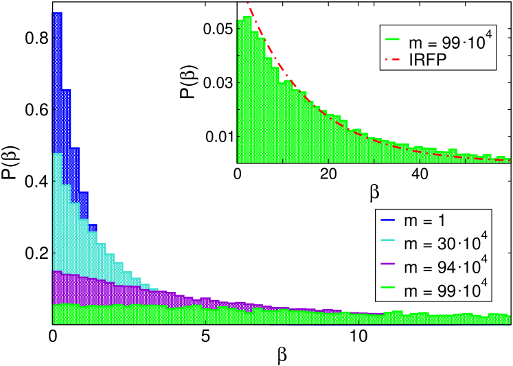
Figure 2: Numerical strong disorder renormalization group: flow of the couplings probability distribution P(β(m))𝑃superscript𝛽𝑚P(\beta^{{}_{(m)}}) as a function of the SDRG step m𝑚m. Different histograms correspond to different m𝑚m. Results are for the Heisenberg spin chain with L=106𝐿superscript106L=10^{6} sites. The width of P(βi(m))𝑃subscriptsuperscript𝛽𝑚𝑖P(\beta^{{}_{(m)}}_{i}) increases upon increasing m𝑚m. Inset: P(β(m))𝑃superscript𝛽𝑚P(\beta^{{}_{(m)}}) for m=99104𝑚99superscript104m=99\cdot 10^{4}, compared with the infinite-randomness fixed point (IRFP) result P(β)=eβ/Γ/Γsuperscript𝑃𝛽superscript𝑒𝛽ΓΓP^{*}(\beta)=e^{-\beta/\Gamma}/\Gamma, (dash-dotted line) with Γ(m)superscriptΓ𝑚\Gamma^{{(m)}} given in (14).

As a preliminary check of the numerical SDRG, we study the flow of the couplings Jisubscript𝐽𝑖J_{i} in (6) as a function of the SDRG step m𝑚m. The results are reported in Fig. 2, where we plot the probability distribution P(βi(m))𝑃superscriptsubscript𝛽𝑖𝑚P(\beta_{i}^{{}_{(m)}}), with βi(m)ln(JM(m)/Ji(m))superscriptsubscript𝛽𝑖𝑚superscriptsubscript𝐽𝑀𝑚subscriptsuperscript𝐽𝑚𝑖\beta_{i}^{{}_{(m)}}\equiv\ln(J_{M}^{{}_{(m)}}/J^{{}_{(m)}}_{i}) (cf. (14)), and JM(m)subscriptsuperscript𝐽𝑚𝑀J^{{}_{(m)}}_{M} the maximum coupling at step m𝑚m. The data are for a finite chain with L=106𝐿superscript106L=10^{6}. The initial values of the couplings are drawn from the box distribution [0,1]01[0,1].

Fig. 2 demonstrates the broadening of the couplings distribution upon increasing the SDRG step m𝑚m, confirming that the SDRG procedure is asymptotically exact at large scale Fisher1994 . The convergence to the universal IRFP distribution P(β)superscript𝑃𝛽P^{*}(\beta) (16) is verified in the inset of Fig. 2.
Refer to caption
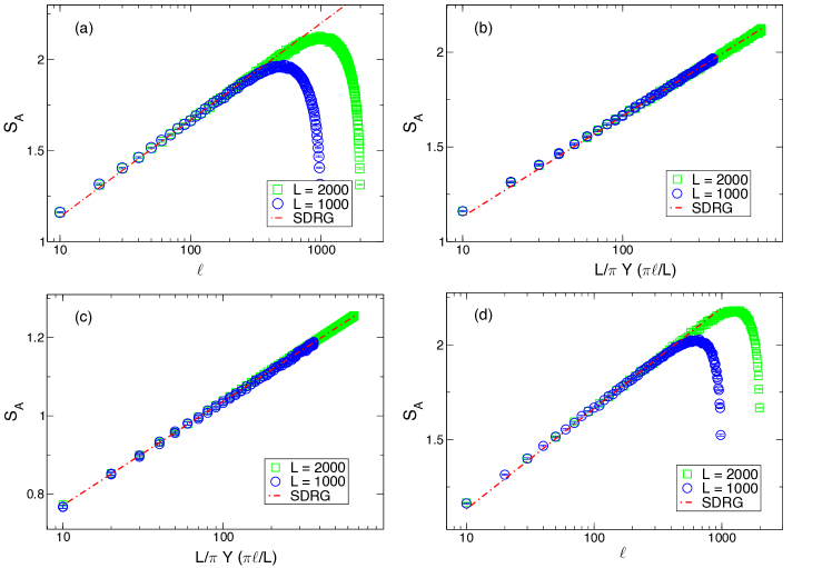
Figure 3: The single interval entanglement entropy for the disordered Heisenberg spin chain. The data correspond to the average over 730007300073000 disorder realizations. Notice that (here and in the following figures) we report also the statistical errors, although the error bars are smaller than the symbol sizes. Different symbols correspond to different chain sizes L𝐿L and dashed dotted lines are one-parameter fit to the analytic prediction from the SDRG. (a) A single interval in a periodic chain: SAsubscript𝑆𝐴S_{A} plotted versus the interval length \ell. (b) Same data as in (a) plotted against the modified chord length (45). (c) A single interval starting from the boundary of a chain with OBC versus the modified chord length (45). (d) A single interval in the bulk of an open chain.

V.2 Single-interval entanglement entropy

Another important check of the validity of the numerical SDRG is provided by the scaling of the single block entanglement entropy. We consider the random XXX𝑋𝑋𝑋XXX chain with both open and periodic boundary conditions. For OBC we expect different scalings depending on whether the block A𝐴A is in the bulk of the chain or whether it touches the boundary. The entanglement entropy SAsubscript𝑆𝐴S_{A} is obtained by determining the number of singlets between A𝐴A and B𝐵B for each realization of the disorder and then by multiplying the average by ln22\ln 2. We report the variance of the distribution as an estimate of statistical error.

Numerical SDRG results for SAsubscript𝑆𝐴S_{A} are shown in Fig. 3 (a)-(d). In all panels the data are for chains of length L=1000𝐿1000L=1000 and L=2000𝐿2000L=2000. The disorder average is over 730007300073000 disorder realizations. We start by considering in panel (a) the block A𝐴A in a periodic chain. For L/2less-than-or-similar-to𝐿2\ell\lesssim L/2, SAsubscript𝑆𝐴S_{A} increases logarithmically as function of the interval length \ell (note the logarithmic scale on the x𝑥x-axis). Instead, for L/2greater-than-or-equivalent-to𝐿2\ell\gtrsim L/2 finite-size effects are visible. The dash-dotted line in the figure is a fit to the expected SDRG result RefaelMoore2004

SA=ln23ln+K,subscript𝑆𝐴23𝐾S_{A}=\frac{\ln 2}{3}\ln\ell+K, (44)

with K𝐾K the only fitting parameter. For L/2less-than-or-similar-to𝐿2\ell\lesssim L/2 the data are in perfect agreement with (44).

As discussed in Ref. FagottiCalabreseMoore2011, , finite-size effects can be taken into account by replacing in (48) the interval length \ell with the modified chord length Lcsubscript𝐿𝑐L_{c} as

LcLπY(πL).subscript𝐿𝑐𝐿𝜋𝑌𝜋𝐿\ell\to L_{c}\equiv\frac{L}{\pi}Y\Big{(}\frac{\pi\ell}{L}\Big{)}. (45)

Here Y(x)𝑌𝑥Y(x) is a symmetric function under xπx𝑥𝜋𝑥x\to\pi-x, which ensures S()=S(L)𝑆𝑆𝐿S(\ell)=S(L-\ell). It has been found that for a single block in a periodic chain, Y(x)𝑌𝑥Y(x) is well approximated by FagottiCalabreseMoore2011

Y(x)=sin(x)(1+43k1sin2(x)),𝑌𝑥𝑥143subscript𝑘1superscript2𝑥Y(x)=\sin(x)\Big{(}1+\frac{4}{3}k_{1}\sin^{2}(x)\Big{)}, (46)

with k10.115similar-tosubscript𝑘10.115k_{1}\sim 0.115. Using (45) in (44) one obtains

SA=ln23ln(Lc)+K.subscript𝑆𝐴23subscript𝐿𝑐𝐾S_{A}=\frac{\ln 2}{3}\ln(L_{c})+K. (47)

Fig. 3 (b) reports the data for SAsubscript𝑆𝐴S_{A} versus Lcsubscript𝐿𝑐L_{c}. The dash-dotted line in Fig. 3 (b) is a fit to (47), and it is in perfect agreement with the SDRG data for all values of \ell confirming the correctness of (47).

In Fig. 3 (c) we consider an open chain with the block A𝐴A starting from the boundary. For a semi-infinite system, the entanglement entropy is expected to be RefaelMoore2004

SA=ln26ln()+K,subscript𝑆𝐴26superscript𝐾S_{A}=\frac{\ln 2}{6}\ln(\ell)+K^{\prime}, (48)

where the prefactor of the logarithm takes into account that subsystem A𝐴A shares only one edge with its complement. This formula indeed describes accurately the data for L/2less-than-or-similar-to𝐿2\ell\lesssim L/2. The finite size and boundary effects can be taken into account again by replacing \ell by a modified chord length (45). We find that the same function Y(x)𝑌𝑥Y(x) in Eq. (46) describes very accurately the data for OBC as shown in Fig. 3 (c). This is a non trivial result since there is no conformal invariance to guarantee the equality of the two finite size scaling functions (i.e. open and periodic) as in the clean case.

Finally in Fig. 3 (d) we consider a block of length \ell in the center of an open chain. For L/2less-than-or-similar-to𝐿2\ell\lesssim L/2 we expect that the block A𝐴A does not feel significantly the presence of the boundary and (44) should describe accurately the data, as evident from the figure. It is instead not obvious how to modify the prediction to take into account finite-size and boundary effects: we only mention that replacing \ell with the modified chord length (46) does not work. This does not come unexpected since also in clean systems the results is more complicated x11 .
Refer to caption
Refer to caption
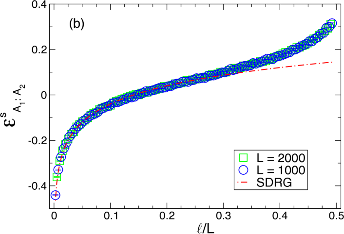
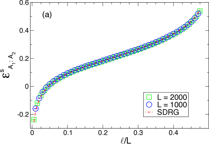
Figure 4: Shifted logarithmic negativity A1:A2ssubscriptsuperscript𝑠:subscript𝐴1subscript𝐴2\mathcal{E}^{s}_{A_{1}:A_{2}} (49) between two adjacent intervals of equal-length \ell in the random Heisenberg chain. A1:A2ssubscriptsuperscript𝑠:subscript𝐴1subscript𝐴2{\cal E}^{s}_{A_{1}:A_{2}} is plotted against /L𝐿\ell/L. The symbols correspond to the average over 730007300073000 disorder realizations. Different symbols correspond to different system sizes. (a): For a periodic chain the data are perfectly described by (50) with only one fitting parameter. (b): For an open chain, we can only use the prediction for the infinite chain which describes well the data as long as Lmuch-less-than𝐿\ell\ll L.

V.3 Logarithmic negativity: Two adjacent intervals

Using the numerical SDRG method, we now study the scaling behavior of the logarithmic negativity A1:A2subscript:subscript𝐴1subscript𝐴2{\cal E}_{A_{1}:A_{2}} between two adjacent intervals A1subscript𝐴1A_{1} and A2subscript𝐴2A_{2} in the random Heisenberg chain. Specifically, we provide robust numerical evidence for (42). The negativity is just obtained from the statistics of the singlets between A1subscript𝐴1A_{1} and A2subscript𝐴2A_{2} and multiplying the resulting average by ln22\ln 2.

In Fig. 4 we report the SDRG data for A1:A2subscript:subscript𝐴1subscript𝐴2{\cal E}_{A_{1}:A_{2}} for two adjacent intervals of the same length \ell. Fig. 4 (a) shows the SDRG results for a periodic chain, while Fig. 4 (b) is for two intervals in the middle of an open chain. We plot the shifted negativity

A1:A2s=A1:A2ln26lnL,subscriptsuperscript𝑠:subscript𝐴1subscript𝐴2subscript:subscript𝐴1subscript𝐴226𝐿{\cal E}^{s}_{A_{1}:A_{2}}={\cal E}_{A_{1}:A_{2}}-\frac{\ln 2}{6}\ln L, (49)

as a function of /L𝐿\ell/L so that data for different chain lengths are expected to collapse on a single scaling curve. This clearly happens for both open and periodic chains. In both cases A1:A2subscript:subscript𝐴1subscript𝐴2{\cal E}_{A_{1}:A_{2}} increases logarithmically for L/4less-than-or-similar-to𝐿4\ell\lesssim L/4, when finite-size effects kick in. Actually, for PBC one can take into account all the finite-size effects by replacing all lengths in (3) with modified chord lengths, obtaining

A1:A2sln26lnYc2(π/L)Yc(2π/L)+k.similar-to-or-equalssubscriptsuperscript𝑠:subscript𝐴1subscript𝐴226superscriptsubscript𝑌𝑐2𝜋𝐿subscript𝑌𝑐2𝜋𝐿𝑘{\cal E}^{s}_{A_{1}:A_{2}}\simeq\frac{\ln 2}{6}\ln\frac{Y_{c}^{2}(\pi\ell/L)}{Y_{c}(2\pi\ell/L)}+k. (50)

The SDRG are perfectly described by this prediction as clear from Fig. 4 (a) where the dashed line is a one parameter fit to (50).

Conversely, for the OBC chain in Fig. 4 (b) there is not a simple modification of the result for infinite chain to take into account the boundary effects, as it was the case also for clean systems ctc-14 . For this reason, in the figure we only report the one-parameter fit to the SDRG prediction for the infinite chain (42) valid for Lmuch-less-than𝐿\ell\ll L.

V.4 Logarithmic negativity: Two disjoint intervals
Refer to caption
Refer to caption
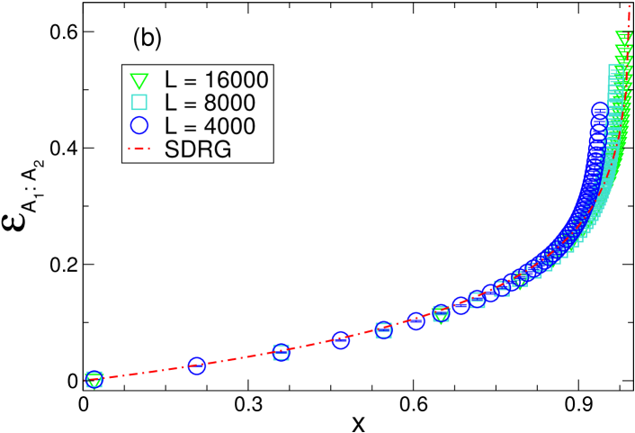
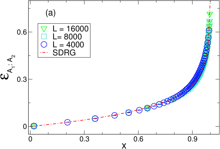
Figure 5: Logarithmic negativity A1:A2subscript:subscript𝐴1subscript𝐴2\mathcal{E}_{A_{1}:A_{2}} between two disjoint intervals of equal length \ell in the random Heisenberg spin chain plotted against the cross ratio x𝑥x. The data are averaged over 730007300073000 disorder realizations. Different symbols correspond to different system sizes. (a): For a periodic chain the cross-ratio x𝑥x is given by (51) and the dashed line is the analytic SDRG prediction (52). (b): For an open chain we consider the infinite volume definition of the cross ratio (5) and the dash-dotted line is the SDRG prediction (52) to which the data tend for large chains.

We finally move to the most interesting case of the logarithmic negativity between two disjoint intervals of equal length \ell at distance r𝑟r. As usual in this section, we compute the negativity from the statistics of the singlets between the two intervals. Our results are reported in Fig. 5 for both periodic and open chains.

In the case of a periodic chain, we plot A1:A2subscript:subscript𝐴1subscript𝐴2\mathcal{E}_{A_{1}:A_{2}} as a function of the cross-ratio x𝑥x (5) in which we have substituted all lengths by the corresponding modified chord lengths, i.e.

x=Yc2(π/L)Yc2(π(+r)/L),𝑥subscriptsuperscript𝑌2𝑐𝜋𝐿subscriptsuperscript𝑌2𝑐𝜋𝑟𝐿x=\frac{Y^{2}_{c}(\pi\ell/L)}{Y^{2}_{c}(\pi(\ell+r)/L)}, (51)

in order to take into account finite-size effects. The SDRG asymptotic prediction for the negativity is given by Eq. (4) which reads

A1:A2=ln26ln(1x).subscript:subscript𝐴1subscript𝐴2261𝑥{\cal E}_{A_{1}:A_{2}}=-\frac{\ln 2}{6}\ln(1-x). (52)

In Fig. 5 (a) the data correspond to a fixed choice of r𝑟r and \ell is running up to (Lr)/2𝐿𝑟2(L-r)/2. It is clear from the figure that the prediction (52) describes incredibly well the numerical data, without any fitting parameter. Notice that x𝑥x close to 00 corresponds to far away intervals and the decay of the negativity is algebraic, in constrast with the exponential behavior of clean systemscalabrese-2012 ; cct-neg-long . Oppositely, the limit x1𝑥1x\to 1 corresponds to very close intervals and the logarithmic divergence is needed to reproduce the adjacent intervals results.

For the case of an open chain, we limit ourselves to consider two intervals centered around the middle of the chain, i.e. A1=[r/2,r/2]subscript𝐴1𝑟2𝑟2A_{1}=[-\ell-r/2,-r/2] and A2=[+r/2,r/2]subscript𝐴2𝑟2𝑟2A_{2}=[\ell+r/2,r/2]. We generate the data by fixing a value of r𝑟r and letting \ell run up to the boundary. In this case, we do not have a prediction which takes into account finite size effects, so we expect Eq. (52) to describe correctly the data for ,rLmuch-less-than𝑟𝐿\ell,r\ll L, i.e. when the effects of the boundary can be neglected. For this reason in Fig. 5 (b) we report the negativity as function of the cross-ratio x𝑥x given by the infinite volume formula x=(/(+r))2𝑥superscript𝑟2x=(\ell/(\ell+r))^{2}. It is evident from the figure that this prediction describes correctly the data for x𝑥x far from 111, as it should. With increasing L𝐿L, the effects of the boundaries becomes less and less relevant and the data get closer to the infinite volume result, as expected.

VI Logarithmic negativity in DMRG simulations
Refer to caption
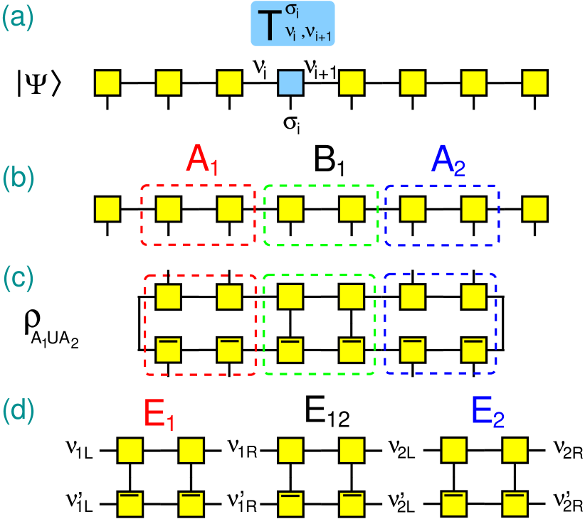
Figure 6: Reduced density matrix with Matrix Product States (MPS) for a chain with L=8𝐿8L=8 sites and open boundary conditions. (a) The MPS representation for a generic wavefunction |ΨketΨ|\Psi\rangle. The basic tensor Tνi,νi+1σisubscriptsuperscript𝑇subscript𝜎𝑖subscript𝜈𝑖subscript𝜈𝑖1T^{\sigma_{i}}_{\nu_{i},\nu_{i+1}} at site i𝑖i of the chain is shown in the shaded box. The vertical leg denotes the physical index σisubscript𝜎𝑖\sigma_{i}, while the horizontal ones are the virtual indices νisubscript𝜈𝑖\nu_{i} (summed over). Tensors in the bulk have rank 333, while at the edges have rank 222. (b) The tripartition of the chain as A1B1A2B2subscript𝐴1subscript𝐵1subscript𝐴2subscript𝐵2A_{1}\cup B_{1}\cup A_{2}\cup B_{2}. A1subscript𝐴1A_{1} and A2subscript𝐴2A_{2} are two equal blocks formed by two spins. The two blocks are at distance two (spins in B1subscript𝐵1B_{1}). (c) The reduced density matrix ρA1A2subscript𝜌subscript𝐴1subscript𝐴2\rho_{A_{1}\cup A_{2}}. Only the tensors living in A1B1A2subscript𝐴1subscript𝐵1subscript𝐴2A_{1}\cup B_{1}\cup A_{2} appear. (d) Definition of the transfer matrices E1subscript𝐸1E_{1}, E2subscript𝐸2E_{2}, E12subscript𝐸12E_{12} corresponding to parts A1subscript𝐴1A_{1}, A2subscript𝐴2A_{2}, and B1subscript𝐵1B_{1} of the chain.

In this section we describe how to calculate the logarithmic negativity in DMRG simulations. We consider a generic 1D1𝐷1D lattice of L𝐿L sites, restricting ourselves to open boundary conditions. On each site i𝑖i of the lattice we consider a local Hilbert space of finite dimension d𝑑d (e.g., for spin-1/2121/2 systems one has d=2𝑑2d=2). A generic wavefunction |ΨketΨ|\Psi\rangle of a pure state is written as a Matrix-Product-State (MPS) as

|Ψ=σ1,,σLTν1σ1Tν1ν2σ2TνLσL|σ1,,σL.ketΨsubscriptsubscript𝜎1subscript𝜎𝐿subscriptsuperscript𝑇subscript𝜎1subscript𝜈1subscriptsuperscript𝑇subscript𝜎2subscript𝜈1subscript𝜈2subscriptsuperscript𝑇subscript𝜎𝐿subscript𝜈𝐿ketsubscript𝜎1subscript𝜎𝐿|\Psi\rangle=\sum\limits_{\sigma_{1},\dots,\sigma_{L}}T^{\sigma_{1}}_{\nu_{1}}T^{\sigma_{2}}_{\nu_{1}\nu_{2}}\cdots T^{\sigma_{L}}_{\nu_{L}}|\sigma_{1},\dots,\sigma_{L}\rangle. (53)

Here σisubscript𝜎𝑖\sigma_{i} with 1id1𝑖𝑑1\leq i\leq d is the so-called physical index representing the states in the local Hilbert space, whereas 1νiχi1subscript𝜈𝑖subscript𝜒𝑖1\leq\nu_{i}\leq\chi_{i} are the virtual indices, with χisubscript𝜒𝑖\chi_{i} the local bond dimension of the MPS. In (53) the sum over the repeated indices νisubscript𝜈𝑖\nu_{i} is assumed, and one has |σ1,σ2,,σL|σ1|σ2|σLketsubscript𝜎1subscript𝜎2subscript𝜎𝐿tensor-productketsubscript𝜎1ketsubscript𝜎2ketsubscript𝜎𝐿|\sigma_{1},\sigma_{2},\dots,\sigma_{L}\rangle\equiv|\sigma_{1}\rangle\otimes|\sigma_{2}\rangle\cdots|\sigma_{L}\rangle, with |σiketsubscript𝜎𝑖|\sigma_{i}\rangle an element of the basis of the Hilbert space at site i𝑖i. At fixed σisubscript𝜎𝑖\sigma_{i}, Tνiνi+1σisubscriptsuperscript𝑇subscript𝜎𝑖subscript𝜈𝑖subscript𝜈𝑖1T^{\sigma_{i}}_{\nu_{i}\nu_{i+1}} is a χi×χisubscript𝜒𝑖subscript𝜒𝑖\chi_{i}\times\chi_{i} matrix, while Tν1σ1subscriptsuperscript𝑇subscript𝜎1subscript𝜈1T^{\sigma_{1}}_{\nu_{1}} and TνLσLsubscriptsuperscript𝑇subscript𝜎𝐿subscript𝜈𝐿T^{\sigma_{L}}_{\nu_{L}} are vectors. The MPS in (53) can be pictorially represented as in Fig. 6 (a), where the boxes denote the tensors Tνi,νi+1σisuperscriptsubscript𝑇subscript𝜈𝑖subscript𝜈𝑖1subscript𝜎𝑖T_{\nu_{i},\nu_{i+1}}^{\sigma_{i}}, and horizontal and vertical legs the virtual and physical indices, respectively. The full system density matrix ρ|ΨΨ|𝜌ketΨbraΨ\rho\equiv|\Psi\rangle\langle\Psi| is obtained as

ρ=σ1,,σLσ1,,σL(Tα1σ1T¯ν1σ1)(Tν1,ν2σ2T¯ν1,ν2σ2)(TνLσLT¯νLσL)|σ1σ1||σLσL|,𝜌subscriptsubscript𝜎1subscript𝜎𝐿superscriptsubscript𝜎1superscriptsubscript𝜎𝐿tensor-productsubscriptsuperscript𝑇subscript𝜎1subscript𝛼1subscriptsuperscript¯𝑇superscriptsubscript𝜎1superscriptsubscript𝜈1subscriptsuperscript𝑇subscript𝜎2subscript𝜈1subscript𝜈2subscriptsuperscript¯𝑇superscriptsubscript𝜎2superscriptsubscript𝜈1superscriptsubscript𝜈2subscriptsuperscript𝑇subscript𝜎𝐿subscript𝜈𝐿subscriptsuperscript¯𝑇superscriptsubscript𝜎𝐿superscriptsubscript𝜈𝐿ketsubscript𝜎1brasuperscriptsubscript𝜎1ketsubscript𝜎𝐿brasuperscriptsubscript𝜎𝐿\rho=\sum\limits_{\begin{subarray}{c}\sigma_{1},\dots,\sigma_{L}\\ \sigma_{1}^{\prime},\dots,\sigma_{L}^{\prime}\end{subarray}}(T^{\sigma_{1}}_{\alpha_{1}}\bar{T}^{\sigma_{1}^{\prime}}_{\nu_{1}^{\prime}})(T^{\sigma_{2}}_{\nu_{1},\nu_{2}}\bar{T}^{\sigma_{2}^{\prime}}_{\nu_{1}^{\prime},\nu_{2}^{\prime}})\cdots\\ \cdots(T^{\sigma_{L}}_{\nu_{L}}\bar{T}^{\sigma_{L}^{\prime}}_{\nu_{L}^{\prime}})|\sigma_{1}\rangle\langle\sigma_{1}^{\prime}|\otimes\cdots\otimes|\sigma_{L}\rangle\langle\sigma_{L}^{\prime}|, (54)

where the bar in T¯νi,νi+1σisubscriptsuperscript¯𝑇subscript𝜎𝑖subscript𝜈𝑖subscript𝜈𝑖1\bar{T}^{\sigma_{i}}_{\nu_{i},\nu_{i+1}} (and correspondingly in the boxes in Fig. 6) denotes the complex conjugation.

Refer to caption
Figure 7: The definition of the tensor N1subscript𝑁1N_{1} (cf. (68)) from the singular value decomposition (SVD) of the transfer matrix E1subscript𝐸1E_{1}. The SVD is performed with respect to the index pairs (ν1L,ν1R)subscript𝜈1𝐿subscript𝜈1𝑅(\nu_{1L},\nu_{1R}) and (ν1L,ν1R)subscriptsuperscript𝜈1𝐿subscriptsuperscript𝜈1𝑅(\nu^{\prime}_{1L},\nu^{\prime}_{1R}). The rhombi denote the diagonal matrix containing the square root of the singular values. The same definition holds for N2subscript𝑁2N_{2}.

VI.1 The partially transposed reduced density matrix

In order to calculate the logarithmic negativity we now introduce a tripartition of the system (Fig. 6) (b) as A1B1A2B2subscript𝐴1subscript𝐵1subscript𝐴2subscript𝐵2A_{1}\cup B_{1}\cup A_{2}\cup B_{2}, where A1subscript𝐴1A_{1} and A2subscript𝐴2A_{2} are the intervals of interest and B1,B2subscript𝐵1subscript𝐵2B_{1},B_{2} the remaining parts. For simplicity we consider the case of two equal-length intervals with 1=2=subscript1subscript2\ell_{1}=\ell_{2}=\ell at mutual distance r𝑟r, and shifted from the left boundary by s𝑠s sites, i.e., A1=[s+1,,s+]subscript𝐴1𝑠1𝑠A_{1}=[s+1,\dots,s+\ell], A2=[s++r+1,,s+r+2]subscript𝐴2𝑠𝑟1𝑠𝑟2A_{2}=[s+\ell+r+1,\dots,s+r+2\ell]. This is illustrated in Fig. 6 (b) for s=1𝑠1s=1, =22\ell=2, and d=2𝑑2d=2. The reduced density matrix ρA1A2subscript𝜌subscript𝐴1subscript𝐴2\rho_{A_{1}\cup A_{2}} is obtained by tracing over the degrees of freedom of B1B2subscript𝐵1subscript𝐵2B_{1}\cup B_{2} in (54) as

ρA1A2=δν1L,ν1Lδν2R,ν2R×{σi,σi:iA1}[F1]ν1L,ν1R{σi}[F¯1]ν1L,ν1R{σi}×{σi,σi:iA2}[F2]ν2L,ν2R{σi}[F¯2]ν2L,ν2R{σi}×[E12]ν1R,ν2Lν1R,ν2LiA1A2|σiσi|,subscript𝜌subscript𝐴1subscript𝐴2subscript𝛿subscript𝜈1𝐿subscriptsuperscript𝜈1𝐿subscript𝛿subscript𝜈2𝑅subscriptsuperscript𝜈2𝑅subscriptconditional-setsubscript𝜎𝑖subscriptsuperscript𝜎𝑖𝑖subscript𝐴1subscriptsuperscriptdelimited-[]subscript𝐹1subscript𝜎𝑖subscript𝜈1𝐿subscript𝜈1𝑅superscriptsubscriptdelimited-[]subscript¯𝐹1subscriptsuperscript𝜈1𝐿subscriptsuperscript𝜈1𝑅subscriptsuperscript𝜎𝑖subscriptconditional-setsubscript𝜎𝑖subscriptsuperscript𝜎𝑖𝑖subscript𝐴2subscriptsuperscriptdelimited-[]subscript𝐹2subscript𝜎𝑖subscript𝜈2𝐿subscript𝜈2𝑅superscriptsubscriptdelimited-[]subscript¯𝐹2subscriptsuperscript𝜈2𝐿subscriptsuperscript𝜈2𝑅subscriptsuperscript𝜎𝑖subscriptsuperscriptdelimited-[]subscript𝐸12subscript𝜈1𝑅subscript𝜈2𝐿subscriptsuperscript𝜈1𝑅subscriptsuperscript𝜈2𝐿subscriptproduct𝑖subscript𝐴1subscript𝐴2ketsubscript𝜎𝑖brasubscriptsuperscript𝜎𝑖\rho_{A_{1}\cup A_{2}}=\delta_{\nu_{1L},\nu^{\prime}_{1L}}\delta_{\nu_{2R},\nu^{\prime}_{2R}}\\ \times\sum\limits_{\begin{subarray}{c}\{\sigma_{i},\sigma^{\prime}_{i}:\,i\in A_{1}\}\end{subarray}}[F_{1}]^{\{\sigma_{i}\}}_{\nu_{1L},\nu_{1R}}[\bar{F}_{1}]_{\nu^{\prime}_{1L},\nu^{\prime}_{1R}}^{\{\sigma^{\prime}_{i}\}}\\ \times\sum\limits_{\begin{subarray}{c}\{\sigma_{i},\sigma^{\prime}_{i}:\,i\in A_{2}\}\end{subarray}}[F_{2}]^{\{\sigma_{i}\}}_{\nu_{2L},\nu_{2R}}[\bar{F}_{2}]_{\nu^{\prime}_{2L},\nu^{\prime}_{2R}}^{\{\sigma^{\prime}_{i}\}}\\ \times[E_{12}]^{\nu_{1R},\nu_{2L}}_{\nu^{\prime}_{1R},\nu^{\prime}_{2L}}\prod\limits_{i\in A_{1}\cup A_{2}}|\sigma_{i}\rangle\langle\sigma^{\prime}_{i}|, (55)

where we defined

[F1]ν1L,ν1R{σi}iA1Tνi,νi+1σi,subscriptsuperscriptdelimited-[]subscript𝐹1subscript𝜎𝑖subscript𝜈1𝐿subscript𝜈1𝑅subscriptproduct𝑖subscript𝐴1subscriptsuperscript𝑇subscript𝜎𝑖subscript𝜈𝑖subscript𝜈𝑖1[F_{1}]^{\{\sigma_{i}\}}_{\nu_{1L},\nu_{1R}}\equiv\prod\limits_{i\in A_{1}}T^{\sigma_{i}}_{\nu_{i},\nu_{i+1}}, (56)

with ν1Lνs+1subscript𝜈1𝐿subscript𝜈𝑠1\nu_{1L}\equiv\nu_{s+1}, ν1Rνs++1subscript𝜈1𝑅subscript𝜈𝑠1\nu_{1R}\equiv\nu_{s+\ell+1} (cf. Fig. 6 (d) for the definition of the indices). A similar definition holds for [F2]ν2L,ν2R{σi}subscriptsuperscriptdelimited-[]subscript𝐹2subscript𝜎𝑖subscript𝜈2𝐿subscript𝜈2𝑅[F_{2}]^{\{\sigma_{i}\}}_{\nu_{2L},\nu_{2R}}. The term δν1L,ν1Lδν2R,ν2Rsubscript𝛿subscript𝜈1𝐿subscriptsuperscript𝜈1𝐿subscript𝛿subscript𝜈2𝑅subscriptsuperscript𝜈2𝑅\delta_{\nu_{1L},\nu^{\prime}_{1L}}\delta_{\nu_{2R},\nu^{\prime}_{2R}} in (55) is because the virtual indices νL,νLsubscript𝜈𝐿subscriptsuperscript𝜈𝐿\nu_{L},\nu^{\prime}_{L} and ν1R,ν1Rsubscript𝜈1𝑅subscriptsuperscript𝜈1𝑅\nu_{1R},\nu^{\prime}_{1R} are contracted. In (55) E12subscript𝐸12E_{12} is the “transfer matrix” of the region connecting the two intervals (B1subscript𝐵1B_{1} in Fig. 6 (c)). The definition of E12subscript𝐸12E_{12} and of the transfer matrices E1subscript𝐸1E_{1}, E2subscript𝐸2E_{2}, which are associated with the two intervals A1subscript𝐴1A_{1} and A2subscript𝐴2A_{2}, are given as

[E1]ν1L,ν1Rν1L,ν1RjA1σjTνj,νj+1σjT¯νj,νj+1σjsubscriptsuperscriptdelimited-[]subscript𝐸1subscript𝜈1𝐿subscript𝜈1𝑅subscriptsuperscript𝜈1𝐿subscriptsuperscript𝜈1𝑅subscriptproduct𝑗subscript𝐴1subscriptsubscript𝜎𝑗subscriptsuperscript𝑇subscript𝜎𝑗subscript𝜈𝑗subscript𝜈𝑗1subscriptsuperscript¯𝑇subscript𝜎𝑗subscriptsuperscript𝜈𝑗subscriptsuperscript𝜈𝑗1\displaystyle[E_{1}]^{\nu_{1L},\nu_{1R}}_{\nu^{\prime}_{1L},\nu^{\prime}_{1R}}\equiv\prod\limits_{j\in A_{1}}\sum_{\sigma_{j}}T^{\sigma_{j}}_{\nu_{j},\nu_{j+1}}\bar{T}^{\sigma_{j}}_{\nu^{\prime}_{j},\nu^{\prime}_{j+1}} (57)
[E2]ν2L,ν2Rν2L,ν2RjA2σjTνj,νj+1σjT¯νj,νj+1σjsubscriptsuperscriptdelimited-[]subscript𝐸2subscript𝜈2𝐿subscript𝜈2𝑅subscriptsuperscript𝜈2𝐿subscriptsuperscript𝜈2𝑅subscriptproduct𝑗subscript𝐴2subscriptsubscript𝜎𝑗subscriptsuperscript𝑇subscript𝜎𝑗subscript𝜈𝑗subscript𝜈𝑗1subscriptsuperscript¯𝑇subscript𝜎𝑗subscriptsuperscript𝜈𝑗subscriptsuperscript𝜈𝑗1\displaystyle[E_{2}]^{\nu_{2L},\nu_{2R}}_{\nu^{\prime}_{2L},\nu^{\prime}_{2R}}\equiv\prod\limits_{j\in A_{2}}\sum_{\sigma_{j}}T^{\sigma_{j}}_{\nu_{j},\nu_{j+1}}\bar{T}^{\sigma_{j}}_{\nu^{\prime}_{j},\nu^{\prime}_{j+1}} (58)
[E12]ν1R,ν2Lν1R,ν2LjB1σjTνj,νj+1σjT¯νj,νj+1σj.subscriptsuperscriptdelimited-[]subscript𝐸12subscript𝜈1𝑅subscript𝜈2𝐿subscriptsuperscript𝜈1𝑅subscriptsuperscript𝜈2𝐿subscriptproduct𝑗subscript𝐵1subscriptsubscript𝜎𝑗subscriptsuperscript𝑇subscript𝜎𝑗subscript𝜈𝑗subscript𝜈𝑗1subscriptsuperscript¯𝑇subscript𝜎𝑗subscriptsuperscript𝜈𝑗subscriptsuperscript𝜈𝑗1\displaystyle[E_{12}]^{\nu_{1R},\nu_{2L}}_{\nu^{\prime}_{1R},\nu^{\prime}_{2L}}\equiv\prod\limits_{j\in B_{1}}\sum_{\sigma_{j}}T^{\sigma_{j}}_{\nu_{j},\nu_{j+1}}\bar{T}^{\sigma_{j}}_{\nu^{\prime}_{j},\nu^{\prime}_{j+1}}. (59)

Notice that all the spin indices are contracted in (57)(58)(59). These definitions are illustrated in Fig. 6 (d).

The computational cost to construct E1,E2,E12subscript𝐸1subscript𝐸2subscript𝐸12E_{1},E_{2},E_{12} is 𝒪(χmax6)𝒪subscriptsuperscript𝜒6𝑚𝑎𝑥{\mathcal{O}}(\chi^{6}_{max}), with χmaxmaxi(χi)subscript𝜒𝑚𝑎𝑥subscriptmax𝑖subscript𝜒𝑖\chi_{max}\equiv\textrm{max}_{i}(\chi_{i}) the largest bond dimension of the MPS. It is convenient to introduce a basis for the Hilbert space of the two intervals A1subscript𝐴1A_{1} and A2subscript𝐴2A_{2} as

|wν1L,ν1R(1)σi:iA1[F1]ν1L,ν1R{σi}jA1|σj,ketsubscriptsuperscript𝑤1subscript𝜈1𝐿subscript𝜈1𝑅subscript:subscript𝜎𝑖𝑖subscript𝐴1subscriptsuperscriptdelimited-[]subscript𝐹1subscript𝜎𝑖subscript𝜈1𝐿subscript𝜈1𝑅subscriptproduct𝑗subscript𝐴1ketsubscript𝜎𝑗\displaystyle|w^{(1)}_{\nu_{1L},\nu_{1R}}\rangle\equiv\sum\limits_{\sigma_{i}:\,i\in A_{1}}[F_{1}]^{\{\sigma_{i}\}}_{\nu_{1L},\nu_{1R}}\prod\limits_{j\in A_{1}}|\sigma_{j}\rangle, (60)
|wν2L,ν2R(2)σi:iA2[F2]ν2L,ν2R{σi}jA2|σj,ketsubscriptsuperscript𝑤2subscript𝜈2𝐿subscript𝜈2𝑅subscript:subscript𝜎𝑖𝑖subscript𝐴2subscriptsuperscriptdelimited-[]subscript𝐹2subscript𝜎𝑖subscript𝜈2𝐿subscript𝜈2𝑅subscriptproduct𝑗subscript𝐴2ketsubscript𝜎𝑗\displaystyle|w^{(2)}_{\nu_{2L},\nu_{2R}}\rangle\equiv\sum\limits_{\sigma_{i}:\,i\in A_{2}}[F_{2}]^{\{\sigma_{i}\}}_{\nu_{2L},\nu_{2R}}\prod\limits_{j\in A_{2}}|\sigma_{j}\rangle, (61)

where the index pairs (ν1L,ν1R)subscript𝜈1𝐿subscript𝜈1𝑅(\nu_{1L},\nu_{1R}) and (ν2L,ν2R)subscript𝜈2𝐿subscript𝜈2𝑅(\nu_{2L},\nu_{2R}) label the different states in the two bases. This allows one to rewrite (55) in the compact form

ρA1A2=δν1L,ν1Lδν2R,ν2R[E12]ν1R,ν2Lν1R,ν2L|wν1L,ν1R(1)wν1L,ν1R(1)||wν2L,ν2R(2)wν2L,ν2R(2)|.subscript𝜌subscript𝐴1subscript𝐴2tensor-productsubscript𝛿subscript𝜈1𝐿subscriptsuperscript𝜈1𝐿subscript𝛿subscript𝜈2𝑅subscriptsuperscript𝜈2𝑅subscriptsuperscriptdelimited-[]subscript𝐸12subscript𝜈1𝑅subscript𝜈2𝐿subscriptsuperscript𝜈1𝑅subscriptsuperscript𝜈2𝐿ketsubscriptsuperscript𝑤1subscript𝜈1𝐿subscript𝜈1𝑅brasubscriptsuperscript𝑤1subscriptsuperscript𝜈1𝐿subscriptsuperscript𝜈1𝑅ketsubscriptsuperscript𝑤2subscript𝜈2𝐿subscript𝜈2𝑅brasubscriptsuperscript𝑤2subscriptsuperscript𝜈2𝐿subscriptsuperscript𝜈2𝑅\rho_{A_{1}\cup A_{2}}=\delta_{\nu_{1L},\nu^{\prime}_{1L}}\delta_{\nu_{2R},\nu^{\prime}_{2R}}[E_{12}]^{\nu_{1R},\nu_{2L}}_{\nu^{\prime}_{1R},\nu^{\prime}_{2L}}\\ |w^{(1)}_{\nu_{1L},\nu_{1R}}\rangle\langle w^{(1)}_{\nu^{\prime}_{1L},\nu^{\prime}_{1R}}|\otimes|w^{(2)}_{\nu_{2L},\nu_{2R}}\rangle\langle w^{(2)}_{\nu^{\prime}_{2L},\nu^{\prime}_{2R}}|. (62)

Notice that now ρA1A2subscript𝜌subscript𝐴1subscript𝐴2\rho_{A_{1}\cup A_{2}} is at most a χmax2×χmax2subscriptsuperscript𝜒2𝑚𝑎𝑥subscriptsuperscript𝜒2𝑚𝑎𝑥\chi^{2}_{max}\times\chi^{2}_{max} matrix. Importantly, for a generic tripartition the vectors |wν1L,ν1R(1)ketsubscriptsuperscript𝑤1subscript𝜈1𝐿subscript𝜈1𝑅|w^{{}_{(1)}}_{\nu_{1L},\nu_{1R}}\rangle and |wν2L,ν2R(2)ketsubscriptsuperscript𝑤2subscript𝜈2𝐿subscript𝜈2𝑅|w^{{}_{(2)}}_{\nu_{2L},\nu_{2R}}\rangle are not orthogonal. Clearly, one has the overlap matrices

wν1L,ν1R(1)|wν1L,ν1R(1)inner-productsubscriptsuperscript𝑤1subscript𝜈1𝐿subscript𝜈1𝑅subscriptsuperscript𝑤1subscriptsuperscript𝜈1𝐿subscriptsuperscript𝜈1𝑅\displaystyle\langle w^{(1)}_{\nu_{1L},\nu_{1R}}|w^{(1)}_{\nu^{\prime}_{1L},\nu^{\prime}_{1R}}\rangle =[E1]ν1L,ν1Rν1L,ν1Rabsentsubscriptsuperscriptdelimited-[]subscript𝐸1subscript𝜈1𝐿subscript𝜈1𝑅subscriptsuperscript𝜈1𝐿subscriptsuperscript𝜈1𝑅\displaystyle=[E_{1}]^{\nu_{1L},\nu_{1R}}_{\nu^{\prime}_{1L},\nu^{\prime}_{1R}} (63)
wν2L,ν2R(2)|wν2L,ν2R(2)inner-productsubscriptsuperscript𝑤2subscript𝜈2𝐿subscript𝜈2𝑅subscriptsuperscript𝑤2subscriptsuperscript𝜈2𝐿subscriptsuperscript𝜈2𝑅\displaystyle\langle w^{(2)}_{\nu_{2L},\nu_{2R}}|w^{(2)}_{\nu^{\prime}_{2L},\nu^{\prime}_{2R}}\rangle =[E2]ν2L,ν2Rν2L,ν2R,absentsubscriptsuperscriptdelimited-[]subscript𝐸2subscript𝜈2𝐿subscript𝜈2𝑅subscriptsuperscript𝜈2𝐿subscriptsuperscript𝜈2𝑅\displaystyle=[E_{2}]^{\nu_{2L},\nu_{2R}}_{\nu^{\prime}_{2L},\nu^{\prime}_{2R}}, (64)

where E1subscript𝐸1E_{1} and E2subscript𝐸2E_{2} are defined in (57) and (58), respectively.

Refer to caption
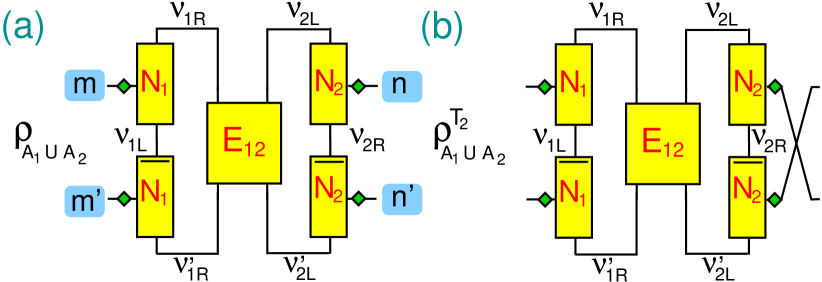
Figure 8: (a) The reduced density matrix of two intervals ρA1A2subscript𝜌subscript𝐴1subscript𝐴2\rho_{A_{1}\cup A_{2}} in the MPS framework. The tensor N1subscript𝑁1N_{1} is defined in Fig. 7 (a similar definition holds for N2subscript𝑁2N_{2}), whereas E12subscript𝐸12E_{12} is as in Fig. 6 (d). The indices are as in (68). The index pairs (m,m)𝑚superscript𝑚(m,m^{\prime}) and (n,n)𝑛superscript𝑛(n,n^{\prime}) refer to interval A1subscript𝐴1A_{1} and A2subscript𝐴2A_{2}, respectively. (b) The partially transposed reduced density matrix ρA1A2T2superscriptsubscript𝜌subscript𝐴1subscript𝐴2subscript𝑇2\rho_{A_{1}\cup A_{2}}^{T_{2}}. Here the partial transposition is performed with respect to subsystem A2subscript𝐴2A_{2}, and it corresponds to the exchange nn𝑛superscript𝑛n\leftrightarrow n^{\prime}.

Interestingly, when the the two intervals A1subscript𝐴1A_{1} and A2subscript𝐴2A_{2} are close to the edges of the chain (this is the geometry considered in Ref. hannu-2008, ) one has that |wν1L,ν1R(1)|wν1R(1)ketsubscriptsuperscript𝑤1subscript𝜈1𝐿subscript𝜈1𝑅ketsubscriptsuperscript𝑤1subscript𝜈1𝑅|w^{{}_{(1)}}_{\nu_{1L},\nu_{1R}}\rangle\to|w^{{}_{(1)}}_{\nu_{1R}}\rangle and |wν2L,ν2R(2)|wν2L(2)ketsubscriptsuperscript𝑤2subscript𝜈2𝐿subscript𝜈2𝑅ketsubscriptsuperscript𝑤2subscript𝜈2𝐿|w^{{}_{(2)}}_{\nu_{2L},\nu_{2R}}\rangle\to|w^{{}_{(2)}}_{\nu_{2L}}\rangle, with |wν1L(1)ketsubscriptsuperscript𝑤1subscript𝜈1𝐿|w^{{}_{(1)}}_{\nu_{1L}}\rangle and |wν2L(2)ketsubscriptsuperscript𝑤2subscript𝜈2𝐿|w^{{}_{(2)}}_{\nu_{2L}}\rangle forming two orthonormal bases. Thus, it is straigthforward to show that ρA1A2subscript𝜌subscript𝐴1subscript𝐴2\rho_{A_{1}\cup A_{2}} is simply given as

ρA1A2=[E12]ν1R,ν2Lν1R,ν2L|wν1R(1)wν1R(1)||wν2L(2)wν2L(2)|.subscript𝜌subscript𝐴1subscript𝐴2tensor-productsubscriptsuperscriptdelimited-[]subscript𝐸12subscript𝜈1𝑅subscript𝜈2𝐿subscriptsuperscript𝜈1𝑅subscriptsuperscript𝜈2𝐿ketsubscriptsuperscript𝑤1subscript𝜈1𝑅brasubscriptsuperscript𝑤1subscriptsuperscript𝜈1𝑅ketsubscriptsuperscript𝑤2subscript𝜈2𝐿brasubscriptsuperscript𝑤2subscriptsuperscript𝜈2𝐿\rho_{A_{1}\cup A_{2}}=[E_{12}]^{\nu_{1R},\nu_{2L}}_{\nu^{\prime}_{1R},\nu^{\prime}_{2L}}\,|w^{{}_{(1)}}_{\nu_{1R}}\rangle\langle w^{{}_{(1)}}_{\nu^{\prime}_{1R}}|\otimes|w^{{}_{(2)}}_{\nu_{2L}}\rangle\langle w^{{}_{(2)}}_{\nu^{\prime}_{2L}}|. (65)

The spectrum of ρA1A2subscript𝜌subscript𝐴1subscript𝐴2\rho_{A_{1}\cup A_{2}} is obtained by diagonalizing E12subscript𝐸12E_{12}, with computational cost χmax6proportional-toabsentsuperscriptsubscript𝜒𝑚𝑎𝑥6\propto\chi_{max}^{6}. Moreover, ρA1A2T2subscriptsuperscript𝜌subscript𝑇2subscript𝐴1subscript𝐴2\rho^{T_{2}}_{A_{1}\cup A_{2}} is obtained from (65) by exchanging ν2Lν2Lsubscript𝜈2𝐿subscriptsuperscript𝜈2𝐿\nu_{2L}\leftrightarrow\nu^{\prime}_{2L}.

For generic tripartitions it is convenient to orthonormalize the vectors |wν1L,ν1R(1)ketsubscriptsuperscript𝑤1subscript𝜈1𝐿subscript𝜈1𝑅|w^{{}_{(1)}}_{\nu_{1L},\nu_{1R}}\rangle and |wν2L,ν2R(2)ketsubscriptsuperscript𝑤2subscript𝜈2𝐿subscript𝜈2𝑅|w^{{}_{(2)}}_{\nu_{2L},\nu_{2R}}\rangle. This can be done via a singular value decomposition (SVD) of the transfer matrices E1subscript𝐸1E_{1} and E2subscript𝐸2E_{2} (cf. (57)(58)). Precisely, given the SVD of E1subscript𝐸1E_{1} as E1=UDVsubscript𝐸1𝑈𝐷superscript𝑉E_{1}=UDV^{\dagger} with U,V𝑈𝑉U,V unitaries and D𝐷D diagonal, the vectors |vm(1)ketsubscriptsuperscript𝑣1𝑚|v^{{}_{(1)}}_{m}\rangle defined as

|vm(1)[N~1]ν1L,ν1Rm|wν1L,ν1R(1),ketsubscriptsuperscript𝑣1𝑚subscriptsuperscriptdelimited-[]subscript~𝑁1𝑚subscript𝜈1𝐿subscript𝜈1𝑅ketsubscriptsuperscript𝑤1subscript𝜈1𝐿subscript𝜈1𝑅|v^{{}_{(1)}}_{m}\rangle\equiv[\widetilde{N}_{1}]^{m}_{\nu_{1L},\nu_{1R}}|w^{{}_{(1)}}_{\nu_{1L},\nu_{1R}}\rangle, (66)

with N~1D12Usubscript~𝑁1superscript𝐷12superscript𝑈\widetilde{N}_{1}\equiv D^{-\frac{1}{2}}U^{\dagger}, are orthonormal. Similarly, for A2subscript𝐴2A_{2} one has the orthonormal vectors

|vm(2)[N~2]ν2L,ν2Rm|wν2L,ν2R(2).ketsubscriptsuperscript𝑣2𝑚subscriptsuperscriptdelimited-[]subscript~𝑁2𝑚subscript𝜈2𝐿subscript𝜈2𝑅ketsubscriptsuperscript𝑤2subscript𝜈2𝐿subscript𝜈2𝑅|v^{{}_{(2)}}_{m}\rangle\equiv[\widetilde{N}_{2}]^{m}_{\nu_{2L},\nu_{2R}}|w^{{}_{(2)}}_{\nu_{2L},\nu_{2R}}\rangle. (67)

Using (66) and (67) one can rewrite ρA1A2subscript𝜌subscript𝐴1subscript𝐴2\rho_{A_{1}\cup A_{2}} as

ρA1A2=([N1]ν1L,ν1Rm[N¯1]ν1L,ν1Rm)([N2]ν2L,ν2Rn[N¯2]ν2L,ν2Rn)×[E12]ν1R,ν2Lν1R,ν2L|vm(1)|vn(2)vm(1)|vn(2)|,subscript𝜌subscript𝐴1subscript𝐴2tensor-producttensor-productsubscriptsuperscriptdelimited-[]subscript𝑁1𝑚subscript𝜈1𝐿subscript𝜈1𝑅subscriptsuperscriptdelimited-[]subscript¯𝑁1superscript𝑚subscript𝜈1𝐿subscriptsuperscript𝜈1𝑅subscriptsuperscriptdelimited-[]subscript𝑁2𝑛subscript𝜈2𝐿subscript𝜈2𝑅subscriptsuperscriptdelimited-[]subscript¯𝑁2superscript𝑛subscriptsuperscript𝜈2𝐿subscript𝜈2𝑅subscriptsuperscriptdelimited-[]subscript𝐸12subscript𝜈1𝑅subscript𝜈2𝐿subscriptsuperscript𝜈1𝑅subscriptsuperscript𝜈2𝐿ketsubscriptsuperscript𝑣1𝑚ketsubscriptsuperscript𝑣2𝑛brasubscriptsuperscript𝑣1superscript𝑚brasuperscriptsubscript𝑣superscript𝑛2\rho_{A_{1}\cup A_{2}}=\\ \big{(}[N_{1}]^{m}_{\nu_{1L},\nu_{1R}}[\bar{N}_{1}]^{m^{\prime}}_{\nu_{1L},\nu^{\prime}_{1R}}\big{)}\big{(}[N_{2}]^{n}_{\nu_{2L},\nu_{2R}}[\bar{N}_{2}]^{n^{\prime}}_{\nu^{\prime}_{2L},\nu_{2R}}\big{)}\\ \times[E_{12}]^{\nu_{1R},\nu_{2L}}_{\nu^{\prime}_{1R},\nu^{\prime}_{2L}}\,\,|v^{{}_{(1)}}_{m}\rangle\otimes|v^{{}_{(2)}}_{n}\rangle\langle v^{{}_{(1)}}_{m^{\prime}}|\otimes\langle v_{n^{\prime}}^{{}_{(2)}}|, (68)

where N1N~11=UD12subscript𝑁1superscriptsubscript~𝑁11𝑈superscript𝐷12N_{1}\equiv\widetilde{N}_{1}^{-1}=UD^{\frac{1}{2}}, and similarly for N2subscript𝑁2N_{2}. The definition of N1subscript𝑁1N_{1} from the SVD of E1subscript𝐸1E_{1} is illustrated in Fig. 7. Formula (68) is illustrated pictorially in Fig. 8 (a). In (68) all the indices are contracted except for m,m,n,n𝑚superscript𝑚𝑛superscript𝑛m,m^{\prime},n,n^{\prime}. Precisely, the index pair (m,m)𝑚superscript𝑚(m,m^{\prime}) refers to subsystem A1subscript𝐴1A_{1}, whereas (n,n)𝑛superscript𝑛(n,n^{\prime}) is associated with A2subscript𝐴2A_{2}. Moreover, one has that n,m,n,m[1,χmax2]𝑛𝑚superscript𝑛superscript𝑚1subscriptsuperscript𝜒2𝑚𝑎𝑥n,m,n^{\prime},m^{\prime}\in[1,\chi^{2}_{max}], implying that the computational cost to evaluate the terms in the round brackets in (68) is χmax7proportional-toabsentsuperscriptsubscript𝜒𝑚𝑎𝑥7\propto\chi_{max}^{7}. However, this can be reduced by considering a truncated SVD of E1subscript𝐸1E_{1} and E2subscript𝐸2E_{2}, i.e., keeping only the p𝑝p (pχmax2much-less-than𝑝superscriptsubscript𝜒𝑚𝑎𝑥2p\ll\chi_{max}^{2}) largest singular values. This relies on the fact that the singular values of E1subscript𝐸1E_{1} and E2subscript𝐸2E_{2} typically decay very quickly. The computational cost is now p2χmax3superscript𝑝2superscriptsubscript𝜒𝑚𝑎𝑥3p^{2}\chi_{max}^{3}. The same trick is used in the implementation of DMRG with periodic boundary conditions pippan-2010 . Finally, from (68) it is straightforward to obtain ρA1A2T2superscriptsubscript𝜌subscript𝐴1subscript𝐴2subscript𝑇2\rho_{A_{1}\cup A_{2}}^{T_{2}} by exchanging nn𝑛superscript𝑛n\leftrightarrow n^{\prime}, as illustrated in Fig. 8 (b).

VI.2 The clean XX𝑋𝑋XX chain: Two adjacent intervals

Refer to caption
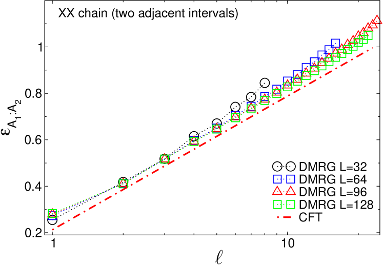
Figure 9: The logarithmic negativity A1:A2subscript:subscript𝐴1subscript𝐴2{\cal E}_{A_{1}:A_{2}} between the two (equal-length) adjacent intervals A1A2subscript𝐴1subscript𝐴2A_{1}\cup A_{2} in the XX𝑋𝑋XX chain. Here the two intervals are at the center of the chain. A1:A2subscript:subscript𝐴1subscript𝐴2{\cal E}_{A_{1}:A_{2}} is plotted against the length of one interval \ell. The symbols are DMRG data for a chain with length up to L=128𝐿128L=128. The dash-dotted line is the CFT prediction 1/4ln141/4\ln\ell in the thermodynamic limit.

Before moving to disordered systems it is worth providing some checks of (68) for clean systems in which all results are under control. To this purpose here we focus on the clean XX𝑋𝑋XX chain

XX=Ji=1L1(SixSi+1x+SiySi+1y)+hi=1LSiz,subscript𝑋𝑋𝐽superscriptsubscript𝑖1𝐿1subscriptsuperscript𝑆𝑥𝑖subscriptsuperscript𝑆𝑥𝑖1subscriptsuperscript𝑆𝑦𝑖subscriptsuperscript𝑆𝑦𝑖1superscriptsubscript𝑖1𝐿superscriptsubscript𝑆𝑖𝑧{\mathcal{H}}_{XX}=J\sum\limits_{i=1}^{L-1}(S^{x}_{i}S^{x}_{i+1}+S^{y}_{i}S^{y}_{i+1})+h\sum\limits_{i=1}^{L}S_{i}^{z}, (69)

with open boundary conditions. We fix J=1𝐽1J=1, considering zero magnetic field h=00h=0. We restrict ourselves to two adjacent intervals at the center of the chain (see Fig. 1 (a)). This corresponds to the trivial transfer matrix [E12]ν1R,ν2Lν1R,ν2L=δν1Rν2Lδν1Rν2Lsubscriptsuperscriptdelimited-[]subscript𝐸12subscript𝜈1𝑅subscript𝜈2𝐿subscriptsuperscript𝜈1𝑅superscriptsubscript𝜈2𝐿subscript𝛿subscript𝜈1𝑅subscript𝜈2𝐿subscript𝛿subscriptsuperscript𝜈1𝑅subscriptsuperscript𝜈2𝐿[E_{12}]^{\nu_{1R},\nu_{2L}}_{\nu^{\prime}_{1R},\nu_{2L}^{\prime}}=\delta_{\nu_{1R}\nu_{2L}}\delta_{\nu^{\prime}_{1R}\nu^{\prime}_{2L}} in (68).

DMRG data for the logarithmic negativity A1:A2subscript:subscript𝐴1subscript𝐴2{\cal E}_{A_{1}:A_{2}} between two adjacent intervals of equal length \ell are reported in Fig. 9. The different symbols correspond to L=32,64,96,128𝐿326496128L=32,64,96,128. In the DMRG simulations we fixed the largest bond dimension to χmax=80subscript𝜒𝑚𝑎𝑥80\chi_{max}=80, and the discarded weight uli2 to ϵ1011similar-toitalic-ϵsuperscript1011\epsilon\sim 10^{-11}. Also, to reduce the computational cost, we considered a truncated SVD of the transfer matrices E1subscript𝐸1E_{1} and E2subscript𝐸2E_{2} (cf. (68) and Fig. 7) fixing p=200𝑝200p=200.

The DMRG data for A1:A2subscript:subscript𝐴1subscript𝐴2{\cal E}_{A_{1}:A_{2}} are plotted against the length of the two intervals \ell (notice the logarithmic scale on the x𝑥x-axis). There are no CFT predictions for A1:A2subscript:subscript𝐴1subscript𝐴2{\cal E}_{A_{1}:A_{2}} in finite systems with open boundary conditions, so we can only use the result for two adjacent intervals in the infinite chain calabrese-2012

A1:A2=c4ln(121+2)+cnst,subscript:subscript𝐴1subscript𝐴2𝑐4subscript1subscript2subscript1subscript2cnst{\cal E}_{A_{1}:A_{2}}=\frac{c}{4}\ln\Big{(}\frac{\ell_{1}\ell_{2}}{\ell_{1}+\ell_{2}}\Big{)}+\textrm{cnst}, (70)

with 1subscript1\ell_{1} and 2subscript2\ell_{2} the lengths of the two intervals, c𝑐c the central charge, and cnst an additive constant. This is expected to describe the data for an open chain as long as 1,2Lmuch-less-thansubscript1subscript2𝐿\ell_{1},\ell_{2}\ll L. This is confirmed for the XX𝑋𝑋XX chain by the data in Fig. 9 in which the dash-dotted line is (70) for 1=2=subscript1subscript2\ell_{1}=\ell_{2}=\ell. While some deviations from (70) are visible for finite L,𝐿L,\ell, the agreement with the CFT prediction (70) becomes progressively better upon increasing L𝐿L, in the region Lmuch-less-than𝐿\ell\ll L.

VII Negativity in the random XX𝑋𝑋XX chain: Some DMRG results

Here we discuss the logarithmic negativity A1:A2subscript:subscript𝐴1subscript𝐴2{\cal E}_{A_{1}:A_{2}} of two adjacent intervals in the random XX𝑋𝑋XX chain (Δ=0Δ0\Delta=0 in (6), see Appendix (A)). To this purpose we perform DMRG simulations, focusing on the disorder distribution Pδ(J)=δ1J1+1/δsubscript𝑃𝛿𝐽superscript𝛿1superscript𝐽11𝛿P_{\delta}(J)=\delta^{-1}J^{-1+1/\delta}, with δ=1/4,1,3/2𝛿14132\delta=1/4,1,3/2. Increasing values of δ𝛿\delta correspond to increasing disorder strength. Specifically, δ=0𝛿0\delta=0 corresponds to the clean case, whereas for δ𝛿\delta\to\infty one recovers the infinite-randomness fixed point (IRFP) distribution (cf. (16)). Our data for A1A2subscriptsubscript𝐴1subscript𝐴2{\cal E}_{A_{1}\cup A_{2}} correspond typically to an average over 103similar-toabsentsuperscript103\sim 10^{3} disorder realizations. Although exact results for the negativity are not yet available, many entanglement-related quantities, such as the entanglement entropy, can be calculated for the random XX𝑋𝑋XX chain, via a mapping to free fermions (cf. Appendix A). Importantly, this provides a reliable way to check the accuracy of DMRG results.

VII.1 Convergence of DMRG

For each disorder realization, a crucial aspect is the convergence of the DMRG method. This depends both on the chain sizes L𝐿L and on the disorder strength δ𝛿\delta. Specifically, we numerically observed that the convergence of DMRG becomes rapidly poor upon increasing L𝐿L or δ𝛿\delta. This is physically expected because the disorder gives rise to a “rough” energy landscape, which makes likely for DMRG to get trapped in a local minimum. This affects severely the convergence because typical DMRG update schemes are local uli2 . This is also related to the exponential small gap Fisher1994 lnΔEL1/2similar-toΔ𝐸superscript𝐿12\ln\Delta E\sim-L^{1/2} of the RS phases.

To check the correctness of the DMRG results, for each disorder realization we compared the data for the half-chain von Neumann entropy with the exact calculation using free-fermion techniques (see Appendix A). We used as a DMRG convergence criterion the matching of the two results within a precision of 103superscript10310^{-3}. We also defined the DMRG convergence rate Rcsubscript𝑅𝑐R_{c} as the fraction of converged DMRG simulations. Only converged disorder configurations were included in the disorder averages.

The fact that Rc<1subscript𝑅𝑐1R_{c}<1 results in a systematic error in the DMRG data. This can be mitigated by using a large number of DMRG sweeps. We typically used nsw100subscript𝑛𝑠𝑤100n_{sw}\approx 100 in our simulations. Moreover, we observed that in each sweep it is crucial to perform a sufficient number of Lanczos iterations nitersubscript𝑛𝑖𝑡𝑒𝑟n_{iter} when locally optimizing the MPS. In our simulations we used niter100subscript𝑛𝑖𝑡𝑒𝑟100n_{iter}\approx 100. Still, we should stress that this is not sufficient to ensure Rc=1subscript𝑅𝑐1R_{c}=1. For instance, we observed that for L=63𝐿63L=63 at δ=1𝛿1\delta=1, using nsw=100subscript𝑛𝑠𝑤100n_{sw}=100 and niter=100subscript𝑛𝑖𝑡𝑒𝑟100n_{iter}=100, one has Rc0.9subscript𝑅𝑐0.9R_{c}\approx 0.9. Finally, to provide reliable error bars for our DMRG results, we always checked that the systematic error was negligible compared with the statistical error arising from the disorder average, providing the latter as our final error estimate.

Fig. 10 (a) shows the comparison between the DMRG data for SAsubscript𝑆𝐴S_{A} (empty symbols in the figure) and the exact results (full symbols) obtained using free-fermion methods (see Appendix A). Data are for δ=3/2𝛿32\delta=3/2, which is the most difficult value of δ𝛿\delta to simulate, and L=16,24𝐿1624L=16,24. The error bars are the statistical errors resulting from the disorder average. In all cases the DMRG results are in agreement with the free-fermion result, within error bars. This suggests that, at least for the von Neumann entropy, the systematic error due to Rc<1subscript𝑅𝑐1R_{c}<1 is negligible compared to the statistical one.
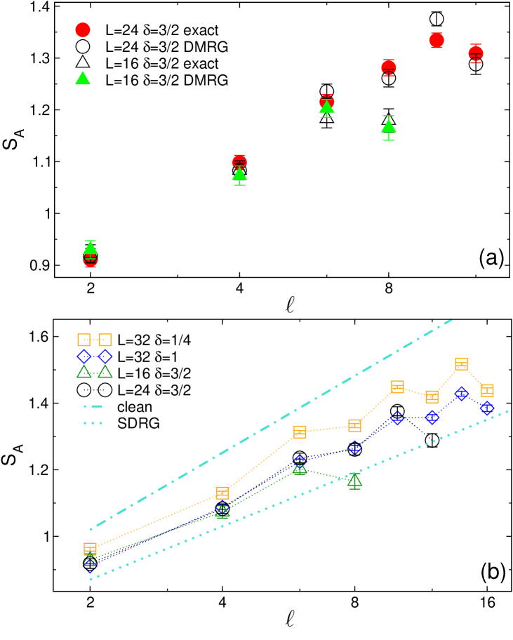
Refer to caption
Figure 10: Entanglement entropy in the random XX spin chain. Panel (a): Check of the DMRG convergence. The von Neumann entropy SAsubscript𝑆𝐴S_{A} for a single interval at the center of an open chain plotted versus the interval length \ell. The empty symbols denote DMRG results for chains with L=16,24𝐿1624L=16,24 and disorder strength δ=3/2𝛿32\delta=3/2. The data are averaged over 103similar-toabsentsuperscript103\sim 10^{3} disorder realizations. The full symbols are exact results obtained using free-fermion techniques. Panel (b): Same geometry as in (a). The symbols are DMRG data for L=16,24,28,32𝐿16242832L=16,24,28,32 and 1/4δ3/214𝛿321/4\leq\delta\leq 3/2. Here δ=0𝛿0\delta=0 and δ𝛿\delta\to\infty correspond to the clean case and the IRFP, respectively. For δ=1𝛿1\delta=1 one has the box distribution. The dash-dotted line is the CFT prediction for δ=0𝛿0\delta=0. The dotted line is the strong disorder renormalization group (SDRG) prediction in the thermodynamic limit.

VII.2 DMRG results

Fig. 10 (b) reports the von Neumann entropy SAsubscript𝑆𝐴S_{A} for the interval A𝐴A at the center of the open chain. The symbols are DMRG data for different δ𝛿\delta and L𝐿L. The dash-dotted line is the CFT result in the clean case SA1/3ln+csimilar-to-or-equalssubscript𝑆𝐴13superscript𝑐S_{A}\simeq 1/3\ln\ell+c^{\prime}, whereas the dotted line is the SDRG result

SAln23ln+const.similar-to-or-equalssubscript𝑆𝐴23constS_{A}\simeq\frac{\ln 2}{3}\ln\ell+{\rm const}. (71)

We recall that the fixed point SDRG is expected to describe the numerical data for any disorder strength, but for asymptotically large \ell and L𝐿L. For finite interval and system lengths, we expect a complicated crossover between the clean and SDRG results, which is more severe for small disorder. In fact, from Fig. 10 (b) it is clear that for the smallest disorder strength (δ=1/4𝛿14\delta=1/4), the data are closer to the clean prediction than to the SDRG one. This does not come unexpected since the crossover between the two fixed points should be regulated by a δ𝛿\delta-dependent crossover length ξδsubscript𝜉𝛿\xi_{\delta}. One should expect that ξδsubscript𝜉𝛿\xi_{\delta}\to\infty for δ0𝛿0\delta\to 0. At any δ𝛿\delta, the IRFP results should be valid only for ,Lξδmuch-greater-than𝐿subscript𝜉𝛿\ell,L\gg\xi_{\delta}. However, the data for δ=1𝛿1\delta=1 and δ=3/2𝛿32\delta=3/2 are almost indistinguishable, signaling that they should be both in the SDRG regime. Indeed, although oscillating corrections are present (as it is well known FagottiCalabreseMoore2011 ), the data are in rough agreement with the SDRG prediction (71) (dotted line). A more quantitative analysis of the entanglement entropy, with a proper robust determination of the prefactor to the logarithmic growth, requires the study of much longer chains as done by means of free fermionic methodslaflorencie-2005 ; FagottiCalabreseMoore2011 . Unfortunately, simulating with DMRG chains of length of the order of hundreds sites and with sufficient statistics is beyond our current capability.
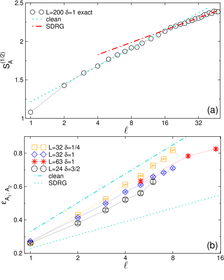
Refer to caption
Figure 11: Entanglement negativity in the random XX spin chain. Panel (a): Rényi entropy SA(1/2)subscriptsuperscript𝑆12𝐴S^{(1/2)}_{A} for a single interval at the center of an open chain plotted versus the interval length \ell. The data (circles) are obtained by means of free-fermionic techniques which allow us to reach large systems sizes (L=200𝐿200L=200). Note the crossover from the scaling of the clean model at short lengths (dotted line) to the SDRG one at large distances (dash-dotted line). Panel (b): The logarithmic negativity A1:A2subscript:subscript𝐴1subscript𝐴2{\cal E}_{A_{1}:A_{2}} for two adjacent intervals of equal length \ell (in the center of an open chain) plotted as a function of \ell. The symbols denote DMRG results for chains with L=16,24,28,32,63𝐿1624283263L=16,24,28,32,63 and disorder strength 1/4δ3/214𝛿321/4\leq\delta\leq 3/2. The data are averaged over 103similar-toabsentsuperscript103\sim 10^{3} disorder realizations. The dash-dotted and dotted lines are the CFT prediction for δ=0𝛿0\delta=0, and the SDRG result, respectively.

Although the data for the entanglement entropy are asymptotically in rough agreement with the prediction of the SDRG already for L=32𝐿32L=32 and δ1similar-to𝛿1\delta\sim 1, this does not imply that the same is true for the negativity, because the crossover between the CFT (clean) and the IRFP fixed points in principle depends on the measured quantity. In order to understand the scaling of the negativity, it is worth to consider the Rényi entropy

SA(1/2)2TrρA1/2,subscriptsuperscript𝑆12𝐴2Trsuperscriptsubscript𝜌𝐴12S^{(1/2)}_{A}\equiv 2{\rm Tr}\rho_{A}^{1/2}, (72)

for a single interval A𝐴A of length \ell at the center of an open chain. Indeed, the negativity for pure states (e.g., for two adjacent intervals with 1+2=Lsubscript1subscript2𝐿\ell_{1}+\ell_{2}=L) coincides with SA(1/2)subscriptsuperscript𝑆12𝐴S^{{}_{(1/2)}}_{A}. Consequently, one could expect the scaling of the negativity to resemble that of SA(1/2)subscriptsuperscript𝑆12𝐴S^{{}_{(1/2)}}_{A}, rather than that of the von Neumann entropy SAsubscript𝑆𝐴S_{A}. In Fig. 11 (a) we report exact numerical data for SA(1/2)superscriptsubscript𝑆𝐴12S_{A}^{{}_{(1/2)}} at δ=1𝛿1\delta=1 obtained by means of free-fermionic techniques, which allow us to reach large systems sizes (L=200𝐿200L=200). Interestingly, the data do not show strong parity effects (i.e., oscillations with the parity of the block size), in contrast with SAsubscript𝑆𝐴S_{A} (the same is true for the negativity in Fig. 11 (b)). Considering these large system sizes we can clearly see the crossover from the scaling of the clean model at short lengths (SA(1/2)1/2lnsimilar-tosubscriptsuperscript𝑆12𝐴12S^{{}_{(1/2)}}_{A}\sim 1/2\ln\ell) to the SDRG one at large distances (SA(1/2)(ln2)/3lnsimilar-tosubscriptsuperscript𝑆12𝐴23S^{{}_{(1/2)}}_{A}\sim(\ln 2)/3\ln\ell). The crossover starts around 15similar-to15\ell\sim 15 and it is fully established around 30similar-to30\ell\sim 30, implying that L120=4×30𝐿120430L\approx 120=4\times 30 would be needed to fully confirm our results. This, however, is not possible with our current DMRG implementation.

Let us, however, consider the logarithmic negativity A1:A2subscript:subscript𝐴1subscript𝐴2{\cal E}_{A_{1}:A_{2}} between the two adjacent intervals. The DMRG data are reported in Fig. 11 (b) for chain sizes up to L=63𝐿63L=63 and for several disorder strengths. The dash-dotted line is the CFT prediction for the clean model A1:A21/4ln()+csimilar-to-or-equalssubscript:subscript𝐴1subscript𝐴214superscript𝑐{\cal E}_{A_{1}:A_{2}}\simeq 1/4\ln(\ell)+c^{\prime} (cf. Fig. 9) while the dotted line is the SDRG result A1:A2(ln2)/6ln()+constsimilar-to-or-equalssubscript:subscript𝐴1subscript𝐴226const{\cal E}_{A_{1}:A_{2}}\simeq(\ln 2)/6\ln(\ell)+{\rm const} (cf. (42)). For δ=1/4𝛿14\delta=1/4, A1A2subscriptsubscript𝐴1subscript𝐴2{\cal E}_{A_{1}\cup A_{2}} grows with a slope similar to the clean case (compare also with Fig. 9). This does not come unexpected since also the results for the entanglement entropy in Fig. 10 (b) for δ=1/4𝛿14\delta=1/4 are affected by a strong crossover. Increasing the strength of the disorder, we observe that for the available subsystems’ sizes the slopes of the negativity appears to reduce, but, as a difference with the entanglement entropy, there is no saturation with δ𝛿\delta and also for δ=3/2𝛿32\delta=3/2 there are still strong crossover effects. This is in complete analogy with what observed for SA(1/2)subscriptsuperscript𝑆12𝐴S^{(1/2)}_{A} in Fig. 11 (a), where the crossover for δ=1𝛿1\delta=1 starts taking place around =1515\ell=15. Indeed, for δ=1𝛿1\delta=1, the last points for L=63𝐿63L=63 with =1515\ell=15 seem to move in the right direction (we cannot access chains of this length for δ=3/2𝛿32\delta=3/2 because of the poor convergence of DMRG for this large disorder). However, these are only very encouraging signals for the correctness of our prediction: we can only conclude that for the system sizes and δ𝛿\delta accessible to DRMG simulations, A1:A2subscript:subscript𝐴1subscript𝐴2{\cal E}_{A_{1}:A_{2}} exhibits deviations from the SDRG prediction (42), which are likely explained as crossover effects. Much larger chain sizes (of the order of L120/130similar-to𝐿120130L\sim 120/130 which are not accessible with our current DMRG implementation), would be needed for the asymptotic IRFP behavior to set in.

VIII Discussion

In this manuscript we considered the scaling behavior of the logarithmic negativity of disordered spin chains in the random singlet phase. Our main results have been already summarized in the Introduction, and for this reason here we only mention some new research directions originating from the present work. First, in the random XX𝑋𝑋XX chain it should be possible by generalizing the results for clean systems eisler-2014 ; coser-2015 ; ctc-16 to treat the moments of the partially-transposed density matrix exactly. By comparing with the analytic results of section III.1, this would allow to provide a more robust check of some of our findings. Another intriguing direction would be to investigate to which extent the relation between the negativity and the mutual information remains valid in more complicated disordered phases. In this respect one possibility would be to focus on the spin-111 random Heisenberg chain refael-2007 . Different physical behavior should also appear in the spin-1/2121/2 Heisenberg chain in which, besides antiferromagnetic couplings, ferromagnetic ones are allowed. Finally, it would be interesting to investigate the scaling of the negativity in excited states of disordered spin models, also in connection with many-boby localization.

IX Acknowledgments

We acknowledge very useful discussions with G. Sierra and K. Agarwal. We also would like to thank M. Collura, F. Pollmann and M. Stoudenmire for very useful insights on the DMRG simulations, and on the ITensor library. All the authors acknowledge support from the ERC under the Starting Grant 279391 EDEQS.

Appendix A The disordered XX𝑋𝑋XX chain

The random XX𝑋𝑋XX chain with open boundary conditions is defined by the Hamiltonian

XX=i=1L1Ji(SixSi+1x+SiySi+1y)+hi=1LSiz,subscript𝑋𝑋superscriptsubscript𝑖1𝐿1subscript𝐽𝑖subscriptsuperscript𝑆𝑥𝑖subscriptsuperscript𝑆𝑥𝑖1subscriptsuperscript𝑆𝑦𝑖subscriptsuperscript𝑆𝑦𝑖1superscriptsubscript𝑖1𝐿superscriptsubscript𝑆𝑖𝑧{\mathcal{H}}_{XX}=\sum\limits_{i=1}^{L-1}J_{i}(S^{x}_{i}S^{x}_{i+1}+S^{y}_{i}S^{y}_{i+1})+h\sum\limits_{i=1}^{L}S_{i}^{z}, (73)

with Six,y,zσix,y,z/2subscriptsuperscript𝑆𝑥𝑦𝑧𝑖superscriptsubscript𝜎𝑖𝑥𝑦𝑧2S^{x,y,z}_{i}\equiv\sigma_{i}^{x,y,z}/2, σiαsuperscriptsubscript𝜎𝑖𝛼\sigma_{i}^{\alpha} being the Pauli matrices acting on site i𝑖i. For periodic boundary conditions one has an extra term in Eq. (73) connecting site L𝐿L with site 111. Hereafter we fix h=00h=0. Here Jisubscript𝐽𝑖J_{i} are uncorrelated random variables. After the Jordan-Wigner transformation

ci=(m=1i1σmz)σixiσiy2,subscript𝑐𝑖superscriptsubscriptproduct𝑚1𝑖1subscriptsuperscript𝜎𝑧𝑚superscriptsubscript𝜎𝑖𝑥𝑖superscriptsubscript𝜎𝑖𝑦2c_{i}=\Big{(}\prod\limits_{m=1}^{i-1}\sigma^{z}_{m}\Big{)}\frac{\sigma_{i}^{x}-i\sigma_{i}^{y}}{2}, (74)

(73) is recast in the free-fermionic form

XX=12i=1L1Ji(cici+1+ci+1ci)+h2i=1L1cici,subscript𝑋𝑋12superscriptsubscript𝑖1𝐿1subscript𝐽𝑖subscriptsuperscript𝑐𝑖subscript𝑐𝑖1subscriptsuperscript𝑐𝑖1subscript𝑐𝑖2superscriptsubscript𝑖1𝐿1subscriptsuperscript𝑐𝑖subscript𝑐𝑖{\mathcal{H}}_{XX}=\frac{1}{2}\sum\limits_{i=1}^{L-1}J_{i}(c^{\dagger}_{i}c_{i+1}+c^{\dagger}_{i+1}c_{i})+\frac{h}{2}\sum\limits_{i=1}^{L-1}c^{\dagger}_{i}c_{i}, (75)

with cisubscript𝑐𝑖c_{i} spinless fermionic operators satisfying the canonical anticommutation relations {cm,cn}=δm,nsubscript𝑐𝑚subscriptsuperscript𝑐𝑛subscript𝛿𝑚𝑛\{c_{m},c^{\dagger}_{n}\}=\delta_{m,n}.

One can now impose that the single-particle eigenstates |ΨqketsubscriptΨ𝑞|\Psi_{q}\rangle (with q𝑞q an integer labelling the different eigenstates) of (75) are of the form

ηq|0|Ψq=iΦq(i)ci|0,superscriptsubscript𝜂𝑞ket0ketsubscriptΨ𝑞subscript𝑖subscriptΦ𝑞𝑖superscriptsubscript𝑐𝑖ket0\eta_{q}^{\dagger}|0\rangle\equiv|\Psi_{q}\rangle=\sum_{i}\Phi_{q}(i)c_{i}^{\dagger}|0\rangle, (76)

with |0ket0|0\rangle the fermion vacuum, Φq(i)subscriptΦ𝑞𝑖\Phi_{q}(i) the eigenstate amplitudes, and ηqsubscript𝜂𝑞\eta_{q} new fermionic operators. The Schrödinger equation, which allows to determine Φq(i)subscriptΦ𝑞𝑖\Phi_{q}(i), becomes

JiΦq(i+1)+Ji1Φq(i1)=2ϵqΦq(i),i,subscript𝐽𝑖subscriptΦ𝑞𝑖1subscript𝐽𝑖1subscriptΦ𝑞𝑖12subscriptitalic-ϵ𝑞subscriptΦ𝑞𝑖for-all𝑖J_{i}\Phi_{q}(i+1)+J_{i-1}\Phi_{q}(i-1)=2\epsilon_{q}\Phi_{q}(i),\quad\forall i, (77)

with JL=0subscript𝐽𝐿0J_{L}=0, and ϵqsubscriptitalic-ϵ𝑞\epsilon_{q} the single-particle eigenvalues. Notice that (77) is the eigenvalue problem for the banded matrix T(Jjδi,j+1+Jj1δi,j1)/2𝑇subscript𝐽𝑗subscript𝛿𝑖𝑗1subscript𝐽𝑗1subscript𝛿𝑖𝑗12T\equiv(J_{j}\delta_{i,j+1}+J_{j-1}\delta_{i,j-1})/2. One can show that the eigenvalues of the matrix T𝑇T are organized in pairs with opposite sign. Precisely, given the amplitude Φ1(i)subscriptΦ1𝑖\Phi_{1}(i) of an eigenvector with ϵq>0subscriptitalic-ϵ𝑞0\epsilon_{q}>0, the amplitudes of the eigenvector with eigenvalue ϵqsubscriptitalic-ϵ𝑞-\epsilon_{q} are obtained as (1)i+1Φq(i)superscript1𝑖1subscriptΦ𝑞𝑖(-1)^{i+1}\Phi_{q}(i).

As a consequence, the ground state |GSket𝐺𝑆|GS\rangle of (73) is in the sector with M=L/2𝑀𝐿2M=L/2 fermions. This is constructed by filling all the negative modes ϵq<0subscriptitalic-ϵ𝑞0\epsilon_{q}<0 as

|GS=ηqMηqM1ηq1|0.ket𝐺𝑆subscriptsuperscript𝜂subscript𝑞𝑀subscriptsuperscript𝜂subscript𝑞𝑀1superscriptsubscript𝜂subscript𝑞1ket0|GS\rangle=\eta^{\dagger}_{q_{M}}\eta^{\dagger}_{q_{M-1}}\cdots\eta_{q_{1}}^{\dagger}|0\rangle. (78)

It is straightforward to derive the anticommutation relations

{ηq,cj}={ηq,cj}=0,subscriptsuperscript𝜂𝑞subscriptsuperscript𝑐𝑗subscript𝜂𝑞subscript𝑐𝑗0\{\eta^{\dagger}_{q},c^{\dagger}_{j}\}=\{\eta_{q},c_{j}\}=0, (79)

and

{ηq,cj}=Φq(j)δk,j,{ηq,cj}=Φ(j)δk,j.formulae-sequencesuperscriptsubscript𝜂𝑞subscript𝑐𝑗subscriptΦ𝑞𝑗subscript𝛿𝑘𝑗subscript𝜂𝑞subscriptsuperscript𝑐𝑗superscriptΦ𝑗subscript𝛿𝑘𝑗\{\eta_{q}^{\dagger},c_{j}\}=\Phi_{q}(j)\delta_{k,j},\quad\{\eta_{q},c^{\dagger}_{j}\}=\Phi^{*}(j)\delta_{k,j}. (80)

Using (79) and (80), the expectation value of the two-point function cicidelimited-⟨⟩subscriptsuperscript𝑐𝑖subscript𝑐𝑖\langle c^{\dagger}_{i}c_{i}\rangle in a generic eigenstate of (73) is given as

cicj=qΦq(i)Φq(j),delimited-⟨⟩superscriptsubscript𝑐𝑖subscript𝑐𝑗subscript𝑞superscriptsubscriptΦ𝑞𝑖subscriptΦ𝑞𝑗\langle c_{i}^{\dagger}c_{j}\rangle=\sum_{q}\Phi_{q}^{*}(i)\Phi_{q}(j), (81)

where the sum if over the q𝑞q single-particle excitations forming the eigenstate.

In order to calculate the entanglemen entropy, let us now introduce a bipartition of the chain into two subsystems as AA¯𝐴¯𝐴A\cup\bar{A}, with A¯¯𝐴\bar{A} denoting the complement of A𝐴A. For free-fermion models, even in presence of disorder, the reduced density matrix ρAsubscript𝜌𝐴\rho_{A} of subsystem A𝐴A is determined by the correlation matrix peschel-1999 ; peschel-1999a ; chung-2001 ; peschel-2004 ; peschel-2004a ; peschel-2009 restricted to A𝐴A as

𝒞ij(A)cicj,subscriptsuperscript𝒞𝐴𝑖𝑗delimited-⟨⟩superscriptsubscript𝑐𝑖subscript𝑐𝑗{\mathcal{C}}^{(A)}_{ij}\equiv\langle c_{i}^{\dagger}c_{j}\rangle, (82)

where i,jA𝑖𝑗𝐴i,j\in A. In particular, given the eigenvalues λksubscript𝜆𝑘\lambda_{k} of 𝒞(A)superscript𝒞𝐴{\mathcal{C}}^{{(A)}}, the entanglement entropy SAsubscript𝑆𝐴S_{A} is given as

SA=k(λklnλk+(1λk)ln(1λk)).subscript𝑆𝐴subscript𝑘subscript𝜆𝑘subscript𝜆𝑘1subscript𝜆𝑘1subscript𝜆𝑘S_{A}=-\sum_{k}(\lambda_{k}\ln\lambda_{k}+(1-\lambda_{k})\ln(1-\lambda_{k})). (83)

References

  • (1) L. Amico, R. Fazio, A. Osterloh, and V. Vedral, Rev. Mod. Phys. 80, 517 (2008).
  • (2) P. Calabrese, J. Cardy, and B. Doyon Eds, J. Phys. A 42, 500301 (2009).
  • (3) J. Eisert, M. Cramer, and M. B. Plenio, Rev. Mod. Phys. 82, 277 (2010).
  • (4) N. Laflorencie, arXiv:1512.03388.
  • (5) A. Peres, Phys. Rev. Lett. 77, 1413 (1996).
  • (6) K  Zyczkowski, P. Horodecki, A. Sanpera, and M. Lewenstein, Phys. Rev. A 58, 883 (1998).
  • (7) K. Zyczkowski, Phys. Rev.  A 60, 3496 (1999).
  • (8) J. Lee, M. S. Kim, Y. J. Park, and S. Lee, J. Mod. Opt. 47, 2151 (2000); J. Eisert and M. B. Plenio, J. Mod. Opt. 46, 145 (1999).
  • (9) G. Vidal and R. F. Werner, Phys. Rev. A 65, 032314 (2002).
  • (10) M. B. Plenio, Phys. Rev. Lett. 95, 090503 (2005); J. Eisert, quant-ph/0610253.
  • (11) P. Calabrese, J. Cardy, and E. Tonni, Phys.  Rev.  Lett. 109, 130502 (2012).
  • (12) P. Calabrese, J. Cardy, and E. Tonni, J. Stat. Mech. P02008 (2013).
  • (13) P. Calabrese, L. Tagliacozzo, and E. Tonni, J. Stat. Mech. (2013) P05002.
  • (14) S. White, Phys. Rev. Lett. 69, 2863 (1992).
  • (15) U. Schollwöck, Rev. Mod. Phys. 77, 259 (2005).
  • (16) U. Schollwöck, Annals of Physics 326, 96 (2011).
  • (17) H. Wichterich, J. Molina-Vilaplana, and S. Bose, Phys. Rev. A 80, 010304 (2009).
  • (18) S. Marcovitch, A. Retzker, M. B. Plenio and B. Reznik, Phys. Rev. A 80, 012325 (2009).
  • (19) H. Wichterich, J. Vidal, and S. Bose, Phys. Rev. A 81, 032311 (2010).
  • (20) P. Calabrese, J. Cardy, and E. Tonni, J. Phys. A 48, 015006 (2015).
  • (21) S. Furukawa, V. Pasquier, and J. Shiraishi, Phys. Rev. Lett. 102, 170602 (2009); P. Calabrese, J. Cardy, and E. Tonni, J. Stat. Mech. P11001 (2009); P. Calabrese, J. Cardy, and E. Tonni, J. Stat. Mech. P01021 (2011); V. Alba, L. Tagliacozzo, and P. Calabrese, J. Stat. Mech. P06012 (2011); A. Coser, L. Tagliacozzo, and E. Tonni, J. Stat. Mech. (2014) P01008.
  • (22) M. Kulaxizi, A. Parnachev, and G. Policastro, JHEP 1409 (2014) 010.
  • (23) A. Coser, E. Tonni and P. Calabrese, J. Stat. Mech. P12017 (2014).
  • (24) M. Hoogeveen and B. Doyon, Nucl. Phys. B 898, 78 (2015).
  • (25) V. Eisler and Z. Zimboras, New J. Phys. 17 053048 (2015).
  • (26) X. Wen, P.-Y. Chang, and S. Ryu, Phys. Rev. B 92, 075109 (2015).
  • (27) M. Rangamani, and M. Rota, JHEP 1410 (2014) 060; E. Perlmutter, M. Rangamani, and M. Rota, Phys. Rev. Lett. 115, 171601 (2015).
  • (28) O. Blondeau-Fournier, O. Castro-Alvaredo, and B. Doyon, arXiv:1508.04026.
  • (29) M. Levin and X.-G. Wen, Phys. Rev. Lett. 96, 110405 (2006).
  • (30) A. Y. Kitaev and J. Preskill, Phys. Rev. Lett. 96, 110404 (2006).
  • (31) Y. A. Lee and G. Vidal, Phys. Rev. A 88, 042318 (2013).
  • (32) C. Castelnovo, Phys. Rev. A 88, 042319 (2013); C. Castelnovo, Phys. Rev. A 89, 042333 (2014).
  • (33) A. Bayat, S. Bose, P. Sodano, and H. Johannesson, Phys. Rev. Lett. 109, 066403 (2012); A. Bayat, P. Sodano, and S. Bose, Phys. Rev. B 81, 064429 (2010).
  • (34) A. Bayat, H. Johannesson, S. Bose, and P. Sodano, Nat. Comm. 5, 3784 (2014).
  • (35) B. Alkurtass, A. Bayat, I. Affleck, S. Bose, H. Johannesson, P. Sodano, E. S. Sorensen, and K. Le Hur, Phys. Rev. B 93, 081106 (2016).
  • (36) A. Coser, E. Tonni, and P. Calabrese, J. Stat. Mech. (2015) P08005.
  • (37) A. Coser, E. Tonni, and P. Calabrese, J. Stat. Mech. (2016) 033116.
  • (38) A. Coser, E. Tonni, and P. Calabrese, arXiv:1511.08328.
  • (39) P.-Y. Chang and X. Wen, arXiv:1601.07492.
  • (40) C. P. Herzog and Y. Wang, arXiv:1601.00678.
  • (41) K. Audenaert, J. Eisert, M. B. Plenio, and R. F. Werner, Phys. Rev. A 66, 042327 (2002).
  • (42) V. Eisler and Z. Zimboras, Phys. Rev. B 93, 115148 (2016).
  • (43) C. De Nobili, A. Coser, and E. Tonni, arXiv:1604.02609.
  • (44) X. Wen, S. Matsura, and S. Ryu, arXiv:1603.08534.
  • (45) V. Alba, J. Stat. Mech. (2013) P05013.
  • (46) C.-M. Chung, V. Alba, L. Bonnes, P. Chen, and A. M. Läuchli, Phys. Rev. B 90, 064401 (2014).
  • (47) C. De Nobili, A. Coser, and E. Tonni, J. Stat. Mech. (2015) P06021
  • (48) G. Refael and J. E. Moore, J. Phys. A 42, 504010 (2009).
  • (49) G. Refael and J. E. Moore, Phys. Rev. Lett. 93, 260602 (2004).
  • (50) N. Laflorencie, Phys. Rev. B 72, 140408(R) (2005).
  • (51) G. De Chiara, S. Montangero, P. Calabrese, and R. Fazio, J. Stat. Mech. (2006) P03001.
  • (52) M. Fagotti, P. Calabrese and J. E. Moore, Phys. Rev. B 83, 045110 (2011).
  • (53) M. Pouranvari and K. Yang, Phys. Rev. B 88, 075123 (2013).
  • (54) G. Ramirez, J. Rodriguez-Laguna, and G. Sierra, J. Stat. Mech. (2014) P07003.
  • (55) R. Santachiara, J. Stat. Mech. (2006) L06002.
  • (56) G. Refael and J. E. Moore, Phys. Rev. B 76, 024419 (2007).
  • (57) J. A. Hoyos, A. P. Vieira, N. Laflorencie, and E. Miranda Phys. Rev. B 76, 174425 (2007).
  • (58) Y.-C. Lin, F. Igloi, and H. Rieger, Phys. Rev. Lett. 99, 147202 (2007).
  • (59) N. E. Bonesteel and K. Yang, Phys. Rev. Lett. 99, 140405 (2007).
  • (60) D. Binosi, G. De Chiara, S. Montangero, and A. Recati Phys. Rev. B 76, 140405 (2007).
  • (61) F. Igloi and Y.-C. Lin, J. Stat. Mech. P06004 (2008).
  • (62) L. Fidkowski, G. Refael, N. E. Bonesteel, and J. E. Moore, Phys. Rev. B 78, 224204 (2008).
  • (63) R. Yu, H. Saleur, and S. Haas, Phys. Rev. B 77, 140402 (2008).
  • (64) J. A. Hoyos, N. Laflorencie, A. P. Vieira, and T. Vojta, Europhys. Lett. 93, 30004 (2011).
  • (65) I. A. Kovacs, and F. Igloi, Phys. Rev. B 80, 214416 (2009) I. A. Kovacs, and F. Igloi, EPL 97, 67009 (2012).
  • (66) J. C. Getelina, F. C. Alcaraz, and J. A. Hoyos, Phys. Rev. B 93, 045136 (2016).
  • (67) J. Rodr guez-Laguna, S. N. Santalla, G. Ramirez, and G. Sierra, 1601.03408.
  • (68) C. K. Burrell and T. J. Osborne, Phys. Rev. Lett. 99, 167201 (2007).
  • (69) F. Igloi, Z. Szatmari, and Y.-C. Lin, Phys. Rev. B 85, 094417 (2012).
  • (70) J. H. Bardarson, F. Pollmann, and J. E. Moore, Phys. Rev. Lett. 109, 017202 (2012).
  • (71) M. Serbyn, Z. Papic, and D. A. Abanin, Phys. Rev. Lett. 110, 260601 (2013).
  • (72) R. Vosk and E. Altman, Phys. Rev. Lett. 112, 217204 (2014); E. Altman and R. Vosk, Ann. Rev. Cond. Matt. Phys. 6, 383 (2015).
  • (73) D. Pekker, G. Refael, E. Altman, E. Demler, and V. Oganesyan, Phys. Rev. X 4, 011052 (2014).
  • (74) Y. Zhao, F. Andraschko, and J. Sirker, arXiv:1602.04380.
  • (75) R. Vasseur and J. E. Moore, Phys. Rev. B 92, 054203 (2015).
  • (76) V. Alba, S. Inglis, and L. Pollet, Phys. Rev. B 93, 094404 (2016).
  • (77) F. Igloi and C. Monthus, Phys. Rep. 412, 277 (2005).
  • (78) Our DMRG code is implemented using the ITENSOR library, http://itensor.org/.
  • (79) S. K. Ma, C. Dasgupta and C. K. Hu, Phys. Rev. Lett. 43, 1434 (1979); C. Dasgupta and S. K. Ma, Phys. Rev. B 22, 1305 (1980).
  • (80) F. Iglói, R. Juhász, and H. Rieger, Phys. Rev. B 61, 11552 (2000).
  • (81) D. S. Fisher, Phys. Rev. B 50, 3799 (1994); D. S. Fisher, Phys. Rev. B 51, 6411 (1995).
  • (82) R. Santos, V. Korepin, and S. Bose, Phys. Rev. A 84, 062307 (2011); R. Santos and V. Korepin, J. Phys. A 45, 125307 (2012). R. Santos and V. Korepin, arXiv:1603.05185.
  • (83) P. Calabrese and J. Cardy, J. Stat. Mech. P06002 (2004).
  • (84) P. Calabrese and J. Cardy, J. Phys. A 42, 504005 (2009).
  • (85) P. Calabrese and A. Lefevre, Phys. Rev. A 78, 032329 (2008).
  • (86) P. Calabrese, M. Mintchev, and E. Vicari, J. Stat. Mech. P09028 (2011).
  • (87) P. Pippan, S. R. White, and H. G. Evertz, Phys. Rev. B 81, 081103(R) (2010).
  • (88) I. Peschel, M. Kaulke, and O. Legeza, Ann. Physik (Lipzig) 8, 153 (1999).
  • (89) I. Peschel and M.-C. Chung, J. Phys. A 32, 8419 (1999).
  • (90) M.-C. Chung and I. Peschel, Phys. Rev. B 64, 064412 (2001).
  • (91) I. Peschel, J. Phys. A 36, L205 (2003).
  • (92) I. Peschel, J. Stat. Mech. (2004) P06004.
  • (93) I. Peschel and V. Eisler, J. Phys. A 42, 504003 (2009).