Langevin equation with fluctuating diffusivity: a two-state model

Abstract

Recently, anomalous subdiffusion, aging, and scatter of the diffusion coefficient have been reported in many single-particle-tracking experiments, though origins of these behaviors are still elusive. Here, as a model to describe such phenomena, we investigate a Langevin equation with diffusivity fluctuating between a fast and a slow state. We assume that the sojourn time distributions of these two states are given by power laws. It is shown that, for a non-equilibrium ensemble, the ensemble-averaged mean square displacement (MSD) shows transient subdiffusion. In contrast, the time-averaged MSD shows normal diffusion, but an effective diffusion coefficient transiently shows aging behavior. The propagator is non-Gaussian for short time, and converges to a Gaussian distribution in a long time limit; this convergence to Gaussian is extremely slow for some parameter values. For equilibrium ensembles, both ensemble-averaged and time-averaged MSDs show only normal diffusion, and thus we cannot detect any traces of the fluctuating diffusivity with these MSDs. Therefore, as an alternative approach to characterize the fluctuating diffusivity, the relative standard deviation (RSD) of the time-averaged MSD is utilized, and it is shown that the RSD exhibits slow relaxation as a signature of the long-time correlation in the fluctuating diffusivity. Furthermore, it is shown that the RSD is related to a non-Gaussian parameter of the propagator. To obtain these theoretical results, we develop a two-state renewal theory as an analytical tool.

I Introduction

Temporal and/or spacial heterogeneities of diffusivity have been reported in various systems such as entangled polymer systems Doi and Edwards (1978); Uneyama et al. (2015), macromolecular diffusion in cells Parry et al. (2014); Leith et al. (2012), and supercooled liquids Yamamoto and Onuki (1998a, b). In Doi and Edwards (1978); Uneyama et al. (2015), it is shown that the center-of-mass motion of reptation dynamics in entangled polymer systems exhibits temporal fluctuations of diffusivity. In Parry et al. (2014), it is reported that particles in a bacterial cytoplasm show a fast and a slow diffusion mode. Similarly, one-dimensional diffusion of a eukaryotic transcription factor along DNA strands has a fast and a slow mode with a local variation of the diffusion coefficient (DC) along the DNA Leith et al. (2012). Molecular dynamics simulations of supercooled liquids reported in Yamamoto and Onuki (1998a, b) show a spatial heterogeneity with roughly two values of diffusivity. As a result of such a spacial heterogeneity of diffusivity, a tagged particle will display temporally fluctuating diffusivity. Also, fluctuating diffusivity would be observed in systems with dynamical heterogeneity (i.e., coexistence of spatial and temporal heterogeneities) such as various glass formers Berthier and Biroli (2011).

Although, as a phenomenological model of single-particle diffusion in spatial and temporal heterogeneities, trap models—i.e., continuous-time random walks (CTRWs) He et al. (2008); Neusius et al. (2009); Weigel et al. (2011); Meroz et al. (2010); Miyaguchi and Akimoto (2011, 2013); Jeon et al. (2013); Schulz et al. (2014) and quenched trap models Bouchaud and Georges (1990)—have been widely used, there have been increasing reports in which trap models fail to describe complex systems with heterogeneities. For example, in Manzo et al. (2015), Manzo et al. show that receptor diffusion on cell membranes is not consistent with the CTRW, and proposed the annealed transit time model (ATTM) which is a Brownian motion with fluctuating diffusivity. In the ATTM, the fluctuating diffusivity is considered to be originated from a local variation of the DC Massignan et al. (2014); Manzo et al. (2015), which is observed in many biological experiments English et al. (2011); Kühn et al. (2011); Cutler et al. (2013); Masson et al. (2014). Moreover, a single polymer in an entangled polymer solution is transiently trapped in a virtual tube comprised by surrounding polymers Doi and Edwards (1978, 1986). Therefore, it is natural to expect that this kind of trapped motion could be described by a CTRW, but this is not the case; instead, the center of mass motion of a single entangled polymer is clearly described by a Langevin equation with fluctuating diffusivity (LEFD) Uneyama et al. (2015). An elaborate simulation study on supercooled liquids in Helfferich et al. (2014a, b) also shows that a tagged particle trajectory slightly deviates from that of CTRW.

In financial mathematics, stochastic differential equations called stochastic volatility models, in which the DC follows other stochastic differential equations, have been extensively studied Stein and Stein (1991); Heston (1993); Scott (1997). Moreover, the underdamped version of the LEFD is analyzed in Rozenfeld et al. (1998); Łuczka et al. (2000), and a special type of the overdamped LEFD, a random walk with diffusing diffusivity (i.e., the DC follows a diffusion equation), is studied recently in Chubynsky and Slater (2014). The ATTM stated above is also a special class of the overdamped LEFD, in which the DC is distributed according to a power law. Along with these models, a two-state LEFD, in which diffusivity fluctuates between two values, $D_{+}$ and $D_{-}$, should be important. This is because, in some experiments including those stated above Yamamoto and Onuki (1998a, b); Knight and Falke (2009); Leith et al. (2012); Parry et al. (2014), it is reported that the DC has roughly two distinct values. Such a two-state LEFD as well as a general form of the overdamped LEFD are studied for the case of equilibrium processes in Uneyama et al. (2015). Here, we study the overdamped LEFD with dichotomous DCs for both equilibrium and non-equilibrium processes. Furthermore, the LEFD is considered to be important for intermittent search Loverdo et al. (2009); Bénichou et al. (2011). In fact, LEFD-like systems with dichotomous DCs are studied as an efficient search strategy for finding a target Reingruber and Holcman (2009, 2010). In these studies, however, Markovian switchings between the DCs are used, whereas we investigate general non-Markovian switchings.

A time-averaged mean square displacement (MSD) is frequently used in experiments Golding and Cox (2006); Burov et al. (2011); Jeon et al. (2011); He et al. (2008) and utilized even in some molecular dynamics simulations Akimoto et al. (2011); Yamamoto et al. (2014, 2015). However, the time-averaged MSD (TMSD) of the LEFD shows only normal diffusion, and thus it is impossible to detect and characterize the fluctuating diffusivity. Besides, the instantaneous DC, $D(t)$, is quite difficult to measure accurately in experiments, since $D(t)$ is multiplied by the thermal noise in the Langevin equation [see Eq. (1)]. Then, how can we characterize $D(t)$ from experimental data? In this article, we show that the relative standard deviation (RSD) of the TMSD is a useful observable to elucidate the fluctuating diffusivity, because the RSD is closely related to the auto-correlation function (ACF), $\left\langle D(t)D(t^{\prime})\right\rangle$. An important point is that the RSD can be calculated from dozens of trajectories $\bm{r}(t)$, and it is not necessary to directly measure $D(t)$.

It is also shown that, in a certain limit ($D_{-}\to 0$), the LEFD shares many properties with the CTRW: subdiffusion in the ensemble-averaged MSD (EMSD), aging in the TMSD, and non-Gaussianity. These properties are common in single-particle-tracking experiments Golding and Cox (2006); Burov et al. (2011); Jeon et al. (2011) and molecular dynamics simulations Akimoto et al. (2011); Yamamoto et al. (2014, 2015), and have been a basis of the CTRW modeling of such systems He et al. (2008); Neusius et al. (2009); Weigel et al. (2011); Meroz et al. (2010); Miyaguchi and Akimoto (2011, 2013); Jeon et al. (2013); Schulz et al. (2014). Therefore, the LEFD is another candidate for modeling such anomalous systems. In this article, various anomalous features mentioned above are checked by numerical simulations for the one-dimensional LEFD (the theoretical results are applicable to $n$-dimensional systems).

Furthermore, we develop a generalized renewal theory as an analytical tool. Systems studied in the usual renewal theory have only a single state Godrèche and Luck (2001), while the LEFD in this article has two states. Therefore, it is necessary to generalize the usual (single-state) renewal theory to the one with two states. Some previous works have already worked on such a generalization Cox (1962); Goychuk and Hänggi (2003); Akimoto and Seki (2015); Uneyama et al. (2015), but, in this article, a much broader framework of the two-state renewal theory, which is also called an alternating renewal theory in Cox (1962), is presented. For example, the fractions of the states, transition probabilities, and probability density functions (PDFs) of a forward recurrence time are investigated.

This paper is organized as follows. In Sec. II, we define the LEFD, switching rules between the two states (i.e., sojourn time PDFs of these states), and equilibrium as well as non-equilibrium ensembles. In Sec. III, analytical results for arbitrary sojourn time PDFs are described, whereas, in Secs. IV– VII, case studies for power-law sojourn time PDFs are presented, and relations between the LEFD and the CTRW are also pointed out here. Finally, Sec. VIII is devoted to a discussion. In the Appendices, we summarize some technical matters, including simulation details and a relation between the RSD and a non-Gaussian parameter.

II Langevin equation with fluctuating Diffusivity

In this section, the LEFD with a fast and a slow diffusion state is defined. Then, we adopt non-Markovian switching rules between the two states through sojourn time PDFs of these states. Also, equilibrium and non-equilibrium initial ensembles are defined with first sojourn time PDFs.

II.1 Definition of the LEFD

The LEFD is given by the following equation:

$$\frac{d\bm{r}(t)}{dt}=\sqrt{2D(t)}\,\bm{\xi}(t),$$ (1)

where $\bm{r}(t)$ is the $n$-dimensional position of the diffusing particle, and $\bm{\xi}(t)$ is Gaussian white noise vector with

$$\left\langle\bm{\xi}(t)\right\rangle=\bm{0},\qquad\left\langle\xi_{i}(t)\xi_{j}(t^{\prime})\right\rangle=\delta_{ij}\delta(t-t^{\prime}).$$ (2)

In contrast, the time-dependent DC, $D(t)$, is allowed to be a non-Markovian stochastic process, whereas we assume that $D(t)$ and $\bm{\xi}(t)$ are statistically independent. Equation (1) is a general definition of an isotropic LEFD. An anisotropic version, which can be utilized to describe the center-of-mass motion of an entangled polymer in a reptation model, is analyzed in Uneyama et al. (2015).

II.2 Two-state system

Figure 1: An example of trajectory $x(t)$ of the two-state LEFD. The regions with shaded and white backgrounds correspond to the fast and the slow modes, respectively. The ratio $D_{+}/D_{-}$ is set as $D_{+}/D_{-}=50$.

In this article, we consider a two-state process, i.e., the state of the system is alternating between two modes, labeled $+$ and $-$. More precisely, it is assumed that the DC is given by $D(t)=D_{+}$ if the state is $+$ at time $t$, and $D(t)=D_{-}$ if the state is $-$ at time $t$. We also assume that $D_{-}\leq D_{+}$ for clarity, though this restriction is not necessary for the theoretical analysis. A trajectory of this two-state LEFD is displayed in Fig. 1.

A switching rule between the two states can be given by sojourn time PDFs of these states. Namely, the sojourn times $\tau$ for $+$ and $-$ states are random variables following different PDFs, $\rho_{+}(\tau)$ and $\rho_{-}(\tau)$. We assume that these PDFs follow power-law distributions (though the results in Sec. III are applicable for arbitrary PDFs):

$$\rho_{\pm}(\tau)\underset{\tau\to\infty}{\simeq}\frac{a_{\pm}}{|\Gamma(-\alpha_{\pm})|\tau^{1+\alpha_{\pm}}},$$ (3)

where $a_{\pm}$ is a scale factor and $\Gamma(-\alpha_{\pm})$ is the gamma function. Asymptotic forms of the Laplace transforms $\hat{\rho}_{\pm}(s):=\int_{0}^{\infty}d\tau\,e^{-\tau s}\rho_{\pm}(\tau)$ at small $s$ are given by

$$\hat{\rho}_{\pm}(s) \underset{s\to 0}{=}1-a_{\pm}s^{\alpha_{\pm}}+O(s)\quad \alpha_{\pm}\in(0,1),$$ (4)

$$\hat{\rho}_{\pm}(s) \underset{s\to 0}{=}1-\mu_{\pm}s+a_{\pm}s^{\alpha_{\pm}}+O(s^{2})\quad \alpha_{\pm}\in(1,2),$$ (5)

where $\mu_{\pm}$ is the mean sojourn time of the state $\pm$ and $O(s^{n})$ is Landau’s notation. Note that $\mu_{\pm}$ does not exist for $\alpha_{\pm}\in(0,1)$. Moreover, in Eqs. (4) and (5), we assume that the sub-leading corrections to Eq. (3) decay faster than $\tau^{-2}$ and $\tau^{-3}$, respectively Bardou et al. (2001); these assumptions are critical in the following analysis , although some important PDFs such as the Lévy’s stable law with $\alpha<1/2$ do not satisfy this assumption.

Here, let us comment on a possible origin of the power-law sojourn time PDFs. It is well known that, for crowded systems such as supercooled liquids, clusters of fast (mobile) and slow (immobile) particles are formed Ediger (2000); Weeks et al. (2000). For example, a slow particle diffuses in a slow cluster, eventually traverses a boundary between clusters, and goes into a fast cluster. Thus, the sojourn time PDF of the slow state may be given by a PDF of the first passage time to the boundary. Such a first passage time PDF in a compact domain is usually given by a power law with an exponential cutoff Redner (2001). This exponential cutoff results in a crossover from anomalous to normal behaviors, but the crossover time could be very long Mantegna and Stanley (1994); Miyaguchi and Akimoto (2011, 2013); thus, the pure power law might be a reasonable assumption (though, this reasoning is still too simplistic, since the clusters themselves are changing with time).

Here, we consider the following six cases for the values of the exponents $\alpha_{+}$ and $\alpha_{-}$:

• : $\alpha_{\pm}\in(0,1)$ with $\alpha_{+}<\alpha_{-}$
  

• : $\alpha_{\pm}\in(0,1)$ with $\alpha_{+}>\alpha_{-}$
  

• : $\alpha_{\pm}\in(1,2)$ with $\alpha_{+}<\alpha_{-}$
  

• : $\alpha_{\pm}\in(1,2)$ with $\alpha_{+}>\alpha_{-}$
  

• : $\alpha_{+}\in(0,1)$ and $\alpha_{-}\in(1,2)$
  

• : $\alpha_{+}\in(1,2)$ and $\alpha_{-}\in(0,1)$

But, essentially, there are only three cases, because, for example, the results for the case (1–2) can be obtained from those of the case (1–1) by substituting the $\pm$ signs in subscripts for $\mp$ signs. Nevertheless, there are qualitative differences between the cases (1–1) and (1–2), and therefore we use the classification into six cases for clarity. We also use a generic term “the case (1)” to refer to both cases (1–1) and (1–2). The same notations such as the “case (2)” and “case (3)” are also used.

II.3 Initial ensembles

Initial ensembles are specified by first sojourn time PDFs. We assume that the process starts at $t=0$, and then, at some time $t=\tau$, the first transition from one state to the other occurs. Let us write the PDF of this first sojourn time, $\tau$, as $w_{+}^{0}(\tau)+w_{-}^{0}(\tau)$. Here, $w_{\pm}^{0}(\tau)$ is defined as $w_{\pm}^{0}(\tau):=p_{\pm}^{0}\rho_{\pm}^{0}(\tau)$, where $p_{\pm}^{0}$ is an initial fraction and $\rho_{\pm}^{0}(\tau)$ is a first sojourn time PDF given that the initial state is $\pm$. We also use a vector notation $\bm{w}^{0}(\tau):=(w_{+}^{0}(\tau),w_{-}^{0}(\tau))$, with which we can completely specify the initial ensembles.

For the equilibrium initial ensemble, we set $\rho_{\pm}^{0}(\tau)=\rho_{\pm}^{\mathrm{eq}}(\tau)$, which is given by its Laplace transform Godrèche and Luck (2001) (see also Appendix B):

$$\hat{\rho}_{\pm}^{\mathrm{eq}}(s)=\frac{1-\hat{\rho}_{\pm}(s)}{\mu_{\pm}s}.$$ (6)

Hence, this PDF exists only if $\mu_{\pm}$ is finite. On the other hand, we set $\rho_{\pm}^{0}(\tau)=\rho_{\pm}(\tau)$ for a non-equilibrium initial ensemble, i.e., the first sojourn time PDF, $\rho_{\pm}^{0}(\tau)$, is the same as the PDF of the second and later sojourn times $\rho_{\pm}(\tau)$ (this is a typical non-equilibrium initial ensemble used in the renewal theory and the CTRW theory).

To define the initial ensembles, we also have to specify initial fractions of the two states, $p_{\pm}^{0}$. In the equilibrium initial ensembles, these fractions are given by (see Appendix B)

$$p_{\pm}^{0}=\frac{\mu_{\pm}}{\mu}=:p_{\pm}^{\mathrm{eq}},$$ (7)

where $\mu$ is defined by $\mu:=\mu_{+}+\mu_{-}$. For the non-equilibrium initial ensembles, we leave $p_{\pm}^{0}\in[0,1]$ arbitrary, because the asymptotic behavior of the system is independent of $p_{\pm}^{0}$ as shown in the following sections.

Thus, the equilibrium ensemble, $\hat{w}_{\pm}^{\mathrm{eq}}(s)$, is given by

$$\hat{w}_{\pm}^{\mathrm{eq}}(s)=p_{\pm}^{\mathrm{eq}}\hat{\rho}_{\pm}^{\mathrm{eq}}(s)=p_{\pm}^{\mathrm{eq}}\frac{1-\hat{\rho}_{\pm}(s)}{\mu_{\pm}s}.$$ (8)

We denote the ensemble average in terms of this equilibrium ensemble as $\left\langle\cdot\right\rangle_{\mathrm{eq}}$. Similarly, the following non-equilibrium ensembles shall be considered:

$$\hat{w}_{\pm}^{\mathrm{neq}}(s)=p_{\pm}^{0}\hat{\rho}_{\pm}(s).$$ (9)

We depict the ensemble average in terms of this non-equilibrium ensemble as $\left\langle\cdot\right\rangle_{\mathrm{neq}}$. Note that, in this notation $\left\langle\cdot\right\rangle_{\mathrm{neq}}$, we do not explicitly show the dependence on the initial fractions $p_{\pm}^{0}$. In numerical simulations, we use two non-equilibrium ensembles: one that starts from $+$ state [i.e., $(p_{+}^{0},p_{-}^{0})=(1,0)$] and the other that starts from $-$ state [i.e., $(p_{+}^{0},p_{-}^{0})=(0,1)$]. When we use the bracket without a subscript $\left\langle\cdot\right\rangle$, it means that the average is taken over an arbitrary initial ensemble $w^{0}_{\pm}(\tau)$.

III General theory

In this section, we derive general formulas for equilibrium and non-equilibrium LEFD with arbitrary sojourn time PDFs, $\rho_{\pm}(\tau)$. In particular, we study fractions of the states, the EMSD, the ensemble-averaged TMSD (ETMSD), the propagator, and the RSD of the TMSD.

III.1 Transition probabilities

We start with transition probabilities $W_{hh^{\prime}}(t|\bm{w}^{0})$ where $h$ and $h^{\prime}$ stand for the states: $h,h^{\prime}=\pm$. More precisely, $W_{hh^{\prime}}(t|\bm{w}^{0})$ is a conditional joint probability that the state is $h$ at time $t=0$ and the state is $h^{\prime}$ at time $t$, given that the process starts with the initial ensemble $\bm{w}^{0}(\tau)$. Let us rewrite $W_{hh^{\prime}}(t|\bm{w}^{0})$ as

$$\begin{split}W_{\pm\pm}(t|\bm{w}^{0})&=\sum_{n=0}^{\infty}Q_{\pm,2n}(t|\bm{w}^{0}),\\ W_{\pm\mp}(t|\bm{w}^{0})&=\sum_{n=1}^{\infty}Q_{\pm,2n-1}(t|\bm{w}^{0}),\end{split}$$ (10)

where $Q_{\pm,n}(t|\bm{w}^{0})$ is a joint probability that the state is $\pm$ at time $t=0$ and there is $n$ transitions until time $t$, given that the process starts with $\bm{w}^{0}(\tau)$. The Laplace transforms are given by

$$\begin{split}\hat{W}_{\pm\pm}(s|\bm{w}^{0})&=\sum_{n=0}^{\infty}\hat{Q}_{\pm,2n}(s|\bm{w}^{0}),\\ \hat{W}_{\pm\mp}(s|\bm{w}^{0})&=\sum_{n=1}^{\infty}\hat{Q}_{\pm,2n-1}(s|\bm{w}^{0}).\end{split}$$ (11)

The probability $Q_{\pm,n}(t|\bm{w}^{0})$ is given as follows:

$$\begin{split}Q_{\pm,0}(t|\bm{w}^{0})&=\mathcal{I}w_{\pm}^{0}(t),\\ Q_{\pm,2n}(t|\bm{w}^{0})&=w_{\pm}^{0}*\rho^{*(n-1)}*\rho_{\mp}*\mathcal{I}\rho_{\pm}(t),\\ Q_{\pm,2n-1}(t|\bm{w}^{0})&=w_{\pm}^{0}*\rho^{*(n-1)}*\mathcal{I}\rho_{\mp}(t),\end{split}$$ (12)

where $n=1,2,\dots$, and an operator $\mathcal{I}$ is defined as $\mathcal{I}f(t):=\int_{t}^{\infty}dt^{\prime}f(t^{\prime})$. Moreover, we define a PDF $\rho(t)$ by a convolution as

$$\rho(t):=\rho_{+}*\rho_{-}(t)=\int_{0}^{t}d\tau\rho_{+}(t-\tau)\rho_{-}(\tau),$$ (13)

and also $n$-time convolution $\rho^{*n}(t)$ as

$$\rho^{*n}(t):=\underbrace{\rho*\dots*\rho}_{n\text{times}}(t).$$ (14)

Then, the Laplace transforms of Eqs. (12) are given by

$$\begin{split}\hat{Q}_{\pm,0}(s|\bm{w}^{0})&=\frac{p_{\pm}^{0}-\hat{w}^{0}_{\pm}(s)}{s},\\[0.0pt] \hat{Q}_{\pm,2n}(s|\bm{w}^{0})&=\hat{w}_{\pm}^{0}(s)\hat{\rho}^{n-1}(s)\hat{\rho}_{\mp}(s)\frac{1-\hat{\rho}_{\pm}(s)}{s},\\[0.0pt] \hat{Q}_{\pm,2n-1}(s|\bm{w}^{0})&=\hat{w}_{\pm}^{0}(s)\hat{\rho}^{n-1}(s)\frac{1-\hat{\rho}_{\mp}(s)}{s},\end{split}$$ (15)

where $n=1,2,\dots$ (A different derivation is given in Appendix A). Putting Eq. (15) into Eq. (11), we have

$$\begin{split}\hat{W}_{\pm\pm}(s|\bm{w}^{0})&=\frac{p_{\pm}^{0}}{s}-\frac{\hat{w}_{\pm}^{0}(s)}{s}\frac{1-\hat{\rho}_{\mp}(s)}{1-\hat{\rho}(s)},\\[0.0pt] \hat{W}_{\pm\mp}(s|\bm{w}^{0})&=\frac{\hat{w}_{\pm}^{0}(s)}{s}\frac{1-\hat{\rho}_{\mp}(s)}{1-\hat{\rho}(s)}.\end{split}$$ (16)

A special case [$p_{+}^{0}=1$, and $\hat{w}_{+}^{0}(s)=\hat{\rho}_{+}^{\mathrm{eq}}(s)$] of these equations is studied in Cox (1962). Note that $\hat{W}_{\pm\pm}(s|\bm{w}^{0})+\hat{W}_{\pm\mp}(s|\bm{w}^{0})=p_{\pm}^{0}/s$, which means the normalization: $W_{\pm\pm}(t|\bm{w}^{0})+W_{\pm\mp}(t|\bm{w}^{0})=p_{\pm}^{0}$.

Inserting Eqs. (7) and (8) into Eq. (16), we have the transition probabilities for the equilibrium processes

$$\begin{split}\hat{W}_{\pm\pm}^{\mathrm{eq}}(s)&:=\hat{W}_{\pm\pm}(s|\bm{w}^{\mathrm{eq}})\\[0.0pt] &=\frac{p_{\pm}^{\mathrm{eq}}}{s}-\frac{1}{\mu s^{2}}\frac{\left[1-\hat{\rho}_{+}(s)\right]\left[1-\hat{\rho}_{-}(s)\right]}{1-\hat{\rho}(s)},\\[0.0pt] \hat{W}_{\pm\mp}^{\mathrm{eq}}(s)&:=\hat{W}_{\pm\mp}(s|\bm{w}^{\mathrm{eq}})\\[0.0pt] &=\frac{1}{\mu s^{2}}\frac{\left[1-\hat{\rho}_{+}(s)\right]\left[1-\hat{\rho}_{-}(s)\right]}{1-\hat{\rho}(s)}.\end{split}$$ (17)

From the second equation, we have $\hat{W}_{+-}^{\mathrm{eq}}(s)=\hat{W}_{-+}^{\mathrm{eq}}(s)$, i.e., the detailed balance holds. The above equations (17) are already reported in Goychuk and Hänggi (2003).

On the other hand, the transition probabilities for the non-equilibrium processes are given by

$$\begin{split}\hat{W}_{\pm\pm}^{\mathrm{neq}}(s)&:=\hat{W}_{\pm\pm}(s|\bm{w}^{\mathrm{neq}})=\frac{p_{\pm}^{0}}{s}\frac{1-\hat{\rho}_{\pm}(s)}{1-\hat{\rho}(s)},\\[0.0pt] \hat{W}_{\pm\mp}^{\mathrm{neq}}(s)&:=\hat{W}_{\pm\mp}(s|\bm{w}^{\mathrm{neq}})=\frac{p_{\pm}^{0}}{s}\frac{1-\hat{\rho}_{\mp}(s)}{1-\hat{\rho}(s)}\hat{\rho}_{\pm}(s),\end{split}$$ (18)

where we inserted Eq. (9) into Eq. (16). From the second equation, we see that $\hat{W}_{+-}^{\mathrm{neq}}(s)\not\equiv\hat{W}_{-+}^{\mathrm{neq}}(s)$, i.e., the detailed balance breaks down.

III.2 Fraction of the state

Ensemble averages of some single-time observables can be obtained from the fractions of the states [e.g., see Eqs. (25) and (27)]. Here, we define the fraction of the state, $p_{\pm}(t|\bm{w}^{0})$, as the probability being in the state $\pm$ at time $t$, given that the initial ensemble is $w^{0}_{\pm}(\tau)$. We have $p_{\pm}(0|\bm{w}^{0})=p_{\pm}^{0}$ and

$$p_{\pm}(t|\bm{w}^{0})=W_{\pm\pm}(t|\bm{w}^{0})+W_{\mp\pm}(t|\bm{w}^{0}).$$ (19)

Therefore, from Eqs. (16) and (19), we have the following general expression for the Laplace transform of the fraction:

$$\hat{p}_{\pm}(s|\bm{w}^{0})=\frac{p_{\pm}^{0}}{s}-\frac{\hat{w}_{\pm}^{0}(s)}{s}\frac{{1-\hat{\rho}_{\mp}(s)}}{1-\hat{\rho}(s)}+\frac{\hat{w}_{\mp}^{0}(s)}{s}\frac{{1-\hat{\rho}_{\pm}(s)}}{1-\hat{\rho}(s)}.$$ (20)

If there exist mean sojourn times $\mu_{\pm}$, we have from Eq. (20)

$$\lim_{s\to 0}sp_{\pm}(s|\bm{w}^{0})=p_{\pm}^{\mathrm{eq}}.$$ (21)

Thus, the fractions $p_{\pm}(t|\bm{w}^{0})$ tend to the equilibrium fractions $p_{\pm}^{\mathrm{eq}}$ as $t\to\infty$. On the other hand, if a mean sojourn time, $\mu_{+}$ or $\mu_{-}$, does not exist, the system never reaches an equilibrium; that is, there is no equilibrium state.

Using Eqs. (17) and (19), we have the fractions for the equilibrium processes as

$$\hat{p}_{\pm}^{\mathrm{eq}}(s):=\hat{p}_{\pm}(s|\bm{w}^{\mathrm{eq}}) =\hat{W}_{\pm\pm}^{\mathrm{eq}}(s)+\hat{W}_{\mp\pm}^{\mathrm{eq}}(s)=\frac{p_{\pm}^{\mathrm{eq}}}{s},$$ (22)

and hence the equilibrium fractions are stationary: $p_{\pm}^{\mathrm{eq}}(t)\equiv p_{\pm}^{\mathrm{eq}}$. On the other hand, from Eqs. (18) and (19), the non-equilibrium fractions, $\hat{p}_{\pm}^{\mathrm{neq}}(s)$, are given by

$$\hat{p}_{\pm}^{\mathrm{neq}}(s):=\hat{p}_{\pm}(s|\bm{w}^{\mathrm{neq}}) =\hat{W}_{\pm\pm}^{\mathrm{neq}}(s)+\hat{W}_{\mp\pm}^{\mathrm{neq}}(s)$$

$$=\frac{p_{\pm}^{0}+p_{\mp}^{0}\hat{\rho}_{\mp}(s)}{s}\frac{1-\hat{\rho}_{\pm}(s)}{1-\hat{\rho}(s)}.$$ (23)

III.3 Ensemble average of the MSD

Using Eq. (1) and $\left\langle\bm{\xi}(t^{\prime})\cdot\bm{\xi}(t^{\prime\prime})\right\rangle=n\delta(t^{\prime}-t^{\prime\prime})$, we have the following expression for the EMSD $\left\langle\delta\bm{r}^{2}(t)\right\rangle$:

$$\left\langle\delta\bm{r}^{2}(t)\right\rangle=2n\int_{0}^{t}dt^{\prime}\left\langle D(t^{\prime})\right\rangle,$$ (24)

where $\delta\bm{r}(t)$ is a displacement $\delta\bm{r}(t):=\bm{r}(t)-\bm{r}(0)$. Hence, the EMSD can be obtained by integrating $\left\langle D(t)\right\rangle$, which is in turn given by

$$\left\langle D(t)\right\rangle =D_{+}p_{+}(t|\bm{w}^{0})+D_{-}p_{-}(t|\bm{w}^{0})$$

$$=D_{-}+(D_{+}-D_{-})p_{+}(t|\bm{w}^{0}).$$ (25)

Then, the Laplace transform is given by

$$\langle\hat{D}(s)\rangle=\frac{D_{-}}{s}+(D_{+}-D_{-})\hat{p}_{+}(s|\bm{w}^{0}),$$ (26)

and therefore, from Eqs. (24) and (26), the Laplace transform of the EMSD is given by

$$\mathcal{L}\left[\left\langle\delta\bm{r}^{2}(t)\right\rangle\right](s)=2n\left[\frac{D_{-}}{s^{2}}+(D_{+}-D_{-})\frac{\hat{p}_{+}(s|\bm{w}^{0})}{s}\right].$$ (27)

Inserting Eq. (20) into Eq. (27), we obtain a general expression of the EMSD in terms of the sojourn time PDFs.

For the equilibrium ensemble, we have from Eq. (25)

$$\langle D(t)\rangle_{\mathrm{eq}}=D_{+}p_{+}^{\mathrm{eq}}+D_{-}p_{-}^{\mathrm{eq}}=:D_{\mathrm{eq}}.$$ (28)

Namely, the equilibrium processes are stationary as expected. From Eq. (24), we have

$$\left\langle\delta\bm{r}^{2}(t)\right\rangle_{\mathrm{eq}}=2nD_{\mathrm{eq}}t,$$ (29)

and hence any equilibrium processes show normal diffusion (this result is consistent with the same property obtained for the underdamped LEFD Rozenfeld et al. (1998); Łuczka et al. (2000)). That is, the second moment of the particle position $\bm{r}(t)$ cannot detect any anomaly, i.e., fluctuating diffusivity, of the equilibrium systems, and therefore it is necessary to study some higher order moments instead.

For the non-equilibrium ensemble, using Eqs. (III.2) and Eq. (25), we have

$$\langle D(t)\rangle_{\mathrm{neq}}=D_{-}+(D_{+}-D_{-})p_{+}^{\mathrm{neq}}(t).$$ (30)

Moreover, by using Eqs. (III.2) and (27), the Laplace transform of the non-equilibrium EMSD is given by

$$\mathcal{L}\left[\left\langle\delta\bm{r}^{2}(t)\right\rangle_{\mathrm{neq}}\right]\!(s)=2n\left[\frac{D_{-}}{s^{2}}+(D_{+}-D_{-})\frac{\hat{p}_{+}^{\mathrm{neq}}(s)}{s}\right]\!.$$ (31)

III.4 Ensemble average of the TMSD

The TMSD, which is frequently used in single particle tracking experiments Golding and Cox (2006); Burov et al. (2011); Jeon et al. (2011); He et al. (2008) as well as in molecular dynamics simulations Akimoto et al. (2011); Yamamoto et al. (2014, 2015), is defined as

$$\overline{\delta\bm{r}^{2}}(\Delta;t):=\frac{1}{t-\Delta}\int_{0}^{t-\Delta}dt^{\prime}\left[\bm{r}(t^{\prime}+\Delta)-\bm{r}(t^{\prime})\right]^{2}.$$ (32)

Here, $t$ is the total measurement time, and $\Delta$ is the lag time. Interestingly, a quantity similar to the TMSD is used as an order parameter for glassy systems Hedges et al. (2009). As with the derivation of Eq. (24), Eq. (32) can be rewritten as

$$\left\langle\overline{\delta\bm{r}^{2}}(\Delta;t)\right\rangle =\frac{1}{t-\Delta}\int_{0}^{t-\Delta}dt^{\prime}\left\langle\left[\bm{r}(t^{\prime}+\Delta)-\bm{r}(t^{\prime})\right]^{2}\right\rangle$$

$$=\frac{2n}{t-\Delta}\int_{0}^{t-\Delta}dt^{\prime}\int_{t^{\prime}}^{t^{\prime}+\Delta}d\tau\left\langle D(\tau)\right\rangle.$$ (33)

For the equilibrium ensembles, using Eqs. (28) and (33), we have

$$\left\langle\overline{\delta\bm{r}^{2}}(\Delta;t)\right\rangle_{\mathrm{eq}}=2nD_{\mathrm{eq}}\Delta,$$ (34)

and hence the ETMSD is equivalent to the EMSD [Eq. (29)].

To deal with general non-equilibrium processes, we rewrite Eq. (33) by using Eq. (24) as

$$\left\langle\overline{\delta\bm{r}^{2}}(\Delta;t)\right\rangle\underset{\Delta\ll t}{\simeq}\frac{1}{t}\int_{0}^{t}dt^{\prime}\Bigl{[}\left\langle\delta\bm{r}^{2}(t^{\prime}+\Delta)\right\rangle-\left\langle\delta\bm{r}^{2}(t^{\prime})\right\rangle\Bigr{]}$$ (35)

where we assume that $\Delta\ll t$. The Laplace transform (with respect to $t$) of the integral in Eq. (35) gives

$$\mathcal{L}\left[t\left\langle\overline{\delta\bm{r}^{2}}(\Delta;t)\right\rangle\right](\Delta;s) \underset{\begin{subarray}{c}s\Delta\ll 1\\[0.85355pt] s\to 0\end{subarray}}{\simeq}\frac{e^{s\Delta}-1}{s}\mathcal{L}\left[\left\langle\delta\bm{r}^{2}(t)\right\rangle\right](s)$$

$$\underset{\begin{subarray}{c}s\Delta\ll 1\\[0.85355pt] s\to 0\end{subarray}}{\simeq}\Delta\mathcal{L}\left[\left\langle\delta\bm{r}^{2}(t)\right\rangle\right](s)$$ (36)

where $s\Delta\ll 1$ is resulted from $\Delta\ll t$. The Laplace inversion gives

$$\left\langle\overline{\delta\bm{r}^{2}}(\Delta;t)\right\rangle\underset{\begin{subarray}{c}\Delta\ll t\\[0.85355pt] t\to\infty\end{subarray}}{\simeq}\frac{\Delta}{t}\Bigl{\langle}\delta\bm{r}^{2}(t)\Bigr{\rangle}.$$ (37)

Therefore, the ETMSD only shows normal diffusion; i.e., the ETMSD depends linearly on the lag time $\Delta$. Hence, the EMSD and ETMSD coincide only if the EMSD shows normal diffusion, otherwise they do not coincide and thus ergodicity breaks down.

For the typical non-equilibrium ensembles given by Eq. (9), we simply rewrite Eq. (37) as

$$\left\langle\overline{\delta\bm{r}^{2}}(\Delta;t)\right\rangle_{\mathrm{neq}}\underset{\begin{subarray}{c}\Delta\ll t\\[0.85355pt] t\to\infty\end{subarray}}{\simeq}\frac{\Delta}{t}\Bigl{\langle}\delta\bm{r}^{2}(t)\Bigr{\rangle}_{\mathrm{neq}}.$$ (38)

Therefore, we can obtain the ETMSD $\langle\overline{\delta\bm{r}^{2}}(\Delta;t)\rangle_{\mathrm{neq}}$ simply from the EMSD $\langle\delta\bm{r}^{2}(t)\rangle_{\mathrm{neq}}$.

III.5 Propagator

The propagator $P_{\pm}(\bm{r},t|\bm{w}^{0})d\bm{r}$ is the probability of finding the particle of $\pm$ state in $(\bm{r},\bm{r}+d\bm{r})$ at time $t$, given that the initial ensemble is $\bm{w}^{0}$. Integral equations for $P_{\pm}(\bm{r},t|\bm{w}^{0})$ can be obtained in a way similar to the analysis for CTRWs Shlesinger et al. (1982); Bouchaud and Georges (1990):

$$P_{\pm}(\bm{r},t|\bm{w}^{0})= \int d\bm{r}^{\prime}G_{\pm}(\bm{r}-\bm{r}^{\prime},t)(\mathcal{I}\rho_{\pm}^{0})(t)P_{\pm}(\bm{r}^{\prime},0|\bm{w}^{0})$$

$$+\int_{0}^{t}dt^{\prime}\int\!d\bm{r}^{\prime} G_{\pm}(\bm{r}-\bm{r}^{\prime},t-t^{\prime})(\mathcal{I}\rho_{\pm})(t-t^{\prime})R_{\pm}(\bm{r}^{\prime},t^{\prime}|\bm{w}^{0}),$$ (39)

$$R_{\pm}(\bm{r},t|\bm{w}^{0})= \int d\bm{r}^{\prime}G_{\mp}(\bm{r}-\bm{r}^{\prime},t)\rho_{\mp}^{0}(t)P_{\mp}(\bm{r}^{\prime},0|\bm{w}^{0})$$

$$+\int_{0}^{t}dt^{\prime}\int d\bm{r}^{\prime} G_{\mp}(\bm{r}-\bm{r}^{\prime},t-t^{\prime})\rho_{\mp}(t-t^{\prime})R_{\mp}(\bm{r}^{\prime},t^{\prime}|\bm{w}^{0}),$$ (40)

where $G_{\pm}(\bm{r},t)$ is the Green function of the diffusion process with the diffusion constant $D_{\pm}$, and $R_{\pm}(\bm{r},t|\bm{w}^{0})d\bm{r}dt$ is the probability of which the particle reaches the domain $(\bm{r},\bm{r}+d\bm{r})$ and becomes $\pm$ state just in the interval $(t,t+dt)$, given that the process starts with $\bm{w}^{0}$. By the Fourier and Laplace transformations , we obtain

$$\breve{P}_{\pm}(\bm{k},s|\bm{w}^{0})= \frac{1-\hat{\rho}_{\pm}^{0}(s_{\pm})}{s_{\pm}}\hat{P}_{\pm}(\bm{k},0|\bm{w}^{0})$$

$$+\frac{1-\hat{\rho}_{\pm}(s_{\pm})}{s_{\pm}}\breve{R}_{\pm}(\bm{k},s|\bm{w}^{0}),$$ (41)

$$\breve{R}_{\pm}(\bm{k},s|\bm{w}^{0})= \hat{\rho}_{\mp}^{0}(s_{\mp})\hat{P}_{\mp}(\bm{k},0|\bm{w}^{0})+\hat{\rho}_{\mp}(s_{\mp})\breve{R}_{\mp}(\bm{k},s|\bm{w}^{0}),$$ (42)

where $s_{\pm}:=s+D_{\pm}\bm{k}^{2}$, and we used the fact that the Fourier transform of $G_{\pm}(\bm{r},t)$ is given by $\hat{G}_{\pm}(\bm{k},t)=e^{-D_{\pm}\bm{k}^{2}t}$ Höfling and Franosch (2013). Here, for simplicity, we assume that the initial position is the origin $\bm{r}(0)=0$, i.e., $P_{\pm}(\bm{r},0|\bm{w}^{0})=p^{0}_{\pm}\delta(\bm{r})$ and $\hat{P}_{\pm}(\bm{k},0|\bm{w}^{0})=p^{0}_{\pm}$. Then, from Eqs. (III.5) and (42), we obtain a general expression for the propagator:

$$\breve{P}_{\pm} (\bm{k},s|\bm{w}^{0})=\frac{1-\hat{\rho}_{\pm}^{0}(s_{\pm})}{s_{\pm}}p_{\pm}^{0}$$

$$+\frac{1-\hat{\rho}_{\pm}(s_{\pm})}{s_{\pm}}\frac{\hat{w}_{\pm}^{0}(s_{\pm})\hat{\rho}_{\mp}(s_{\mp})+\hat{w}_{\mp}^{0}(s_{\mp})}{1-\hat{\rho}_{+}(s_{+})\hat{\rho}_{-}(s_{-})}.$$ (43)

Using Eqs. (7), (8) and (III.5), we have the equilibrium propagator, $\breve{P}_{\pm}^{\mathrm{eq}}(\bm{k},s):=\breve{P}_{\pm}(\bm{k},s|\bm{w}^{\mathrm{eq}})$, as

$$\breve{P}_{\pm}^{\mathrm{eq}}(\bm{k},s)=\frac{p_{\pm}}{s_{\pm}}+\frac{[1-\hat{\rho}_{+}(s_{+})][1-\hat{\rho}_{-}(s_{-})]}{\mu s_{\pm}[1-\hat{\rho}_{+}(s_{+})\hat{\rho}_{-}(s_{-})]}\left(\frac{1}{s_{\mp}}-\frac{1}{s_{\pm}}\right).$$ (44)

Note that if $D_{+}=D_{-}$, the second term vanishes and the system shows normal diffusion with the Gaussian propagator all the time. Therefore, the second term is the contribution from the fluctuating diffusivity, and the propagator is non-Gaussian in general if $D_{+}\neq D_{-}$. For the equilibrium processes, using the asymptotic relation given in Eq. (5), and assuming that $s_{\pm}\ll 1$ along with $s\sim\bm{k}^{2}\ll 1$ (i.e., a hydrodynamic limit), we have

$$\breve{P}_{\pm}^{\mathrm{eq}}(\bm{k},s)\underset{\begin{subarray}{c}s,\bm{k}\to 0\\[-0.85355pt] s\sim\bm{k}^{2}\end{subarray}}{\simeq}\frac{p_{\pm}^{\mathrm{eq}}}{s+D_{\mathrm{eq}}\bm{k}^{2}}.$$ (45)

Thus, in this hydrodynamic limit, the propagators for both $+$ and $-$ states become Gaussian Höfling and Franosch (2013). Note also that, the sum of the propagators, $\breve{P}_{+}^{\mathrm{eq}}(\bm{k},s)+\breve{P}_{-}^{\mathrm{eq}}(\bm{k},s)$, becomes a Gaussian distribution; this is the propagator of the diffusion process with the diffusion constant $D_{\mathrm{eq}}$.

From Eqs. (9) and (III.5), we have the non-equilibrium propagator, $\breve{P}_{\pm}^{\mathrm{neq}}(\bm{k},s):=\breve{P}_{\pm}(\bm{k},s|\bm{w}^{\mathrm{neq}})$, as

$$\breve{P}_{\pm}^{\mathrm{neq}}(\bm{k},s)\underset{\begin{subarray}{c}s,\bm{k}\to 0\\[-0.85355pt] s\sim\bm{k}^{2}\end{subarray}}{\simeq}\frac{1}{s_{\pm}}\frac{1-\hat{\rho}_{\pm}(s_{\pm})}{1-\hat{\rho}_{+}(s_{+})\hat{\rho}_{-}(s_{-})},$$ (46)

where an approximation $p_{\mp}^{0}\hat{\rho}_{\mp}(s_{\mp})+p_{\pm}^{0}\simeq 1$ is used. Thus, Eq. (46) is exact only for its leading order terms.

III.6 Relative standard deviation of TMSD

As presented in the previous subsections, both EMSD and ETMSD exhibit normal diffusion for equilibrium processes. Thus, with these MSDs, we cannot extract any information on fluctuating diffusivity. To characterize such anomaly, we may have to consider some higher order moments. Here, we study the RSD of TMSD:

$$\Sigma(\Delta;t|\bm{w}^{0}):=\frac{\sqrt{\bigl{\langle}\bigr{|}\overline{\delta\bm{r}^{2}}(\Delta;t)\bigr{|}^{2}-\bigl{\langle}\overline{\delta\bm{r}^{2}}(\Delta;t)\bigr{\rangle}^{2}\bigr{\rangle}}}{\bigl{\langle}\overline{\delta\bm{r}^{2}}(\Delta;t)\bigr{\rangle}}.$$ (47)

Note that $\Sigma(\Delta;t|\bm{w}^{0})$ is a fourth moment of $\bm{r}(t^{\prime})$. It will be shown that, for the equilibrium process, this RSD is related to the ACF, $\left\langle D(t)D(0)\right\rangle_{\mathrm{eq}}$ [see Eq. (60)]. The RSD analysis is useful even for the non-equilibrium processes, because the RSD is related to non-Gaussianity of the propagator (see Appendix E).

By assuming that $\Delta$ is much smaller than the characteristic correlation time of $D(t)$, we can make the analysis relatively simple (This formal approximation is represented by the symbol ”$\approx$”). For example, under this assumption, we have $\left\langle D(\tau)\right\rangle\approx\left\langle D(t^{\prime})\right\rangle$ in the integrand of Eq. (33), and thus obtain

$$\left\langle\overline{\delta\bm{r}^{2}}(\Delta;t)\right\rangle\approx\frac{2n\Delta}{t-\Delta}\int_{0}^{t-\Delta}dt^{\prime}\left\langle D(t^{\prime})\right\rangle.$$ (48)

This equation is consistent with Eqs. (24) and (37) [though Eq. (37) is valid even if $\Delta$ is larger than the correlation time of $D(t)$]. In this subsection, we analyze the RSD on the basis of this approximation.

With the help of Wick’s theorem,

$$\sum_{i,j}\left\langle\xi_{i}(s)\xi_{i}(s^{\prime})\xi_{j}(u)\xi_{j}(u^{\prime})\right\rangle =$$

$$n^{2}\delta(s-s^{\prime})\delta(u-u^{\prime})+ 2n\delta(s-u^{\prime})\delta(s^{\prime}-u),$$ (49)

the second moment of the TMSD can be approximated as follows:

$$\left\langle\bigl{|}\overline{\delta\bm{r}^{2}}(\Delta;t)\bigr{|}^{2}\right\rangle =\frac{2}{(t-\Delta)^{2}}\int_{0}^{t-\Delta}dt^{\prime}\int_{0}^{t^{\prime}}dt^{\prime\prime}\left\langle\left[\bm{r}(t^{\prime}+\Delta)-\bm{r}(t^{\prime})\right]^{2}\left[\bm{r}(t^{\prime\prime}+\Delta)-\bm{r}(t^{\prime\prime})\right]^{2}\right\rangle.$$

$$\approx\frac{8n\Delta^{2}}{(t-\Delta)^{2}}\!\!\int_{0}^{t-\Delta}\!\!\!\!\!\!\!dt^{\prime}\!\!\int_{0}^{t^{\prime}}\!\!\!dt^{\prime\prime}\!\left[n\left\langle D(t^{\prime})D(t^{\prime\prime})\right\rangle+\frac{2(t^{\prime\prime}-t^{\prime}+\Delta)^{2}}{\Delta^{2}}I(t^{\prime}\leq t^{\prime\prime}+\Delta)\left\langle D^{2}(t^{\prime})\right\rangle\right]$$ (50)

$$=\frac{8n^{2}\Delta^{2}}{(t-\Delta)^{2}}\left[\int_{0}^{t-\Delta}dt^{\prime}\int_{0}^{t^{\prime}}dt^{\prime\prime}\left\langle D(t^{\prime})D(t^{\prime\prime})\right\rangle+\frac{2\Delta}{3n}\int_{0}^{t-\Delta}dt^{\prime}\left\langle D^{2}(t^{\prime})\right\rangle\right],$$ (51)

where $I(\dots)=1$ if the inside of the bracket is satisfied, 0 otherwise. In deriving Eq. (50), we used approximations

$$\int_{t^{\prime}}^{t^{\prime}+\Delta}ds\int_{t^{\prime\prime}}^{t^{\prime\prime}+\Delta}du\left\langle D(s)D(u)\right\rangle\approx\left\langle D(t^{\prime})D(t^{\prime\prime})\right\rangle\Delta^{2},$$ (52)

and $\left\langle D(s)D(u)\right\rangle\approx\left\langle D^{2}(t^{\prime})\right\rangle$ for $s,u\in(t^{\prime}-\Delta,t^{\prime}+\Delta)$. These approximations are justified, because $\Delta$ is much smaller than the characteristic correlation time of $D(t)$.

Inserting Eqs. (48) and (51) into Eq. (47), we obtain

$$\Sigma^{2}(\Delta;t|\bm{w}^{0})\underset{\Delta\ll t}{\approx}\Sigma_{\mathrm{id}}^{2}(\Delta;t|\bm{w}^{0})+\Sigma_{\mathrm{ex}}^{2}(t|\bm{w}^{0}),$$ (53)

with

$$\Sigma^{2}_{\mathrm{id}}(\Delta;t|\bm{w}^{0}) :=\frac{4\Delta}{3n}\frac{\displaystyle\int_{0}^{t}dt^{\prime}\left\langle D^{2}(t^{\prime})\right\rangle}{\displaystyle\int_{0}^{t}dt^{\prime}\int_{0}^{t}dt^{\prime\prime}\left\langle D(t^{\prime})\right\rangle\!\left\langle D(t^{\prime\prime})\right\rangle},$$ (54)

$$\Sigma^{2}_{\mathrm{ex}}(t|\bm{w}^{0}) :=\frac{\displaystyle\int_{0}^{t}dt^{\prime}\int_{0}^{t}dt^{\prime\prime}\left\langle\delta D(t^{\prime})\delta D(t^{\prime\prime})\right\rangle}{\displaystyle\int_{0}^{t}dt^{\prime}\int_{0}^{t}dt^{\prime\prime}\left\langle D(t^{\prime})\right\rangle\!\left\langle D(t^{\prime\prime})\right\rangle},$$ (55)

where $\delta D(t^{\prime})$ is defined by $\delta D(t^{\prime}):=D(t^{\prime})-\left\langle D(t^{\prime})\right\rangle$. If there is no fluctuating diffusivity, then $\Sigma^{2}_{\mathrm{ex}}(t|\bm{w}^{0})=0$ since $\delta D(t)=0$, and thus only $\Sigma^{2}_{\mathrm{id}}(\Delta;t|\bm{w}^{0})$ contributes the RSD. Namely, $\Sigma^{2}_{\mathrm{id}}(\Delta;t|\bm{w}^{0})$ is the RSD for single-mode diffusion processes, and thus we call this term as an ideal part. In contrast, a contribution from the fluctuating diffusivity is represented by $\Sigma^{2}_{\mathrm{ex}}(t|\bm{w}^{0})$, an excess part of the RSD.

For the cases studied in this paper [Eqs. (4) and (5)], the leading term of the ideal part $\Sigma_{\mathrm{id}}^{2}(\Delta;t|\bm{w}^{0})$ at large $t$ is estimated as

$$\Sigma_{\mathrm{id}}^{2}(\Delta;t|\bm{w}^{0})\underset{t\to\infty}{=}O\left(\frac{1}{t}\right).$$ (56)

This can be obtained as follows. First, note that $\left\langle D^{2}(t)\right\rangle=D_{+}^{2}p_{+}(t|\bm{w}^{0})+D_{-}^{2}p_{-}(t|\bm{w}^{0})$, and this is the same as Eq. (25) except that $D_{\pm}$ is replaced by $D_{\pm}^{2}$. Therefore, $2n\int_{0}^{t-\Delta}dt^{\prime}\left\langle D^{2}(t^{\prime})\right\rangle$ has the same form as the EMSD $\left\langle\delta\bm{r}^{2}(t)\right\rangle=2n\int_{0}^{t}dt^{\prime}\left\langle D(t^{\prime})\right\rangle$ except that $D_{\pm}$ is replaced by $D_{\pm}^{2}$. As shown in Secs. III.3 and V, the EMSD shows only normal diffusion $\left\langle\delta\bm{r}^{2}(t)\right\rangle=O(t)$ as $t\to\infty$ [see Eqs. (29), (89), (90), (94), (95), (99), and (100)]. Therefore, we can conclude that

$$2n\int_{0}^{t-\Delta}dt^{\prime}\left\langle D^{2}(t^{\prime})\right\rangle\underset{t\to\infty}{=}O(t)$$ (57)

From these facts and Eq. (54), we obtain (56).

In particular, for the case (3), we shall obtain $\int_{0}^{t-\Delta}dt^{\prime}\left\langle D(t^{\prime})\right\rangle=D_{\pm}t+O(t^{\alpha_{\pm}})$ [Eqs. (99) and (100)]. Thus, we have $\int_{0}^{t-\Delta}dt^{\prime}\left\langle D^{2}(t^{\prime})\right\rangle=D_{\pm}^{2}t+O(t^{\alpha_{\pm}})$, and whereby obtaining from Eq. (54)

$$\Sigma_{\mathrm{id}}^{2}(\Delta;t|\bm{w}^{\mathrm{neq}})\underset{t\to\infty}{=}\frac{4\Delta}{3nt}+O\left(t^{\alpha_{\pm}-2}\right)$$ (58)

where $\alpha_{\pm}\in(0,1)$.

Thus, the leading term of the ideal part $\Sigma^{2}_{\mathrm{id}}(\Delta;t|\bm{w}^{0})$ is of the order of $1/t$. Therefore, if the excess part $\Sigma_{\mathrm{ex}}^{2}(t|\bm{w}^{0})$ shows slow relaxation $1/t^{\beta}$ with $\beta\in(0,1)$, this part $\Sigma_{\mathrm{ex}}^{2}(t|\bm{w}^{0})$ is dominant over the ideal part. In contrast, if the excess part $\Sigma_{\mathrm{ex}}^{2}(t|\bm{w}^{0})$ shows fast relaxation $1/t^{\beta}$ with $\beta>1$, the ideal part $\Sigma_{\mathrm{id}}^{2}(\Delta;t|\bm{w}^{0})$ is dominant over the excess part. The former is actually the case for almost all the cases studied in this article except a couple of narrow parameter regions in case (3) [see Secs. VII.4 and VII.5].

III.6.1 equilibrium processes

For the equilibrium processes, we have from Eq. (55)

$$\Sigma^{2}_{\mathrm{ex}}(t|\bm{w}^{\mathrm{eq}})\simeq\frac{2}{t^{2}}\int_{0}^{t}dt^{\prime}(t-t^{\prime})\frac{\left\langle\delta D(t^{\prime})\delta D(0)\right\rangle_{\mathrm{eq}}}{D_{\mathrm{eq}}^{2}},$$ (59)

where we assumed that $\left\langle\delta D(t^{\prime})\delta D(t^{\prime\prime})\right\rangle_{\mathrm{eq}}$ depends only on the time lag $t^{\prime}-t^{\prime\prime}$ (see Appendix C for a proof). Let us rewrite the above equation as

$$\left\langle\delta D(t)\delta D(0)\right\rangle_{\mathrm{eq}}\underset{}{\simeq}\frac{D_{\mathrm{eq}}^{2}}{2}\frac{\partial^{2}}{\partial t^{2}}\left[t^{2}\Sigma^{2}_{\mathrm{ex}}(t|\bm{w}^{\mathrm{eq}})\right].$$ (60)

As shown in Sec. VII.1, the excess RSD, $\Sigma^{2}_{\mathrm{ex}}(t|\bm{w}^{\mathrm{eq}})$, decays slower than $1/t$ for the case (2), and thus $\Sigma^{2}(\Delta;t|\bm{w}^{\mathrm{eq}})\approx\Sigma^{2}_{\mathrm{ex}}(t|\bm{w}^{\mathrm{eq}})$. Therefore, Eq. (60) implies that we can obtain the ACF, $\left\langle\delta D(t)\delta D(0)\right\rangle_{\mathrm{eq}}$, by measuring the RSD, $\Sigma^{2}(\Delta;t|\bm{w}^{\mathrm{eq}})$. It is important that the RSD and $D_{\mathrm{eq}}$ can be calculated from dozens of trajectories. By contrast, the instantaneous DC, $D(t)$, is difficult to measure directly in experiments. The Laplace transform of Eq. (59) with respect to $t$ becomes

$$\mathcal{L}\left[t^{2}\Sigma^{2}_{\mathrm{ex}}(t|\bm{w}^{\mathrm{eq}})\right](s)\simeq\frac{2}{D_{\mathrm{eq}}^{2}}\frac{\langle\delta\hat{D}(s)\delta D(0)\rangle_{\mathrm{eq}}}{s^{2}}$$ (61)

Moreover, if ${\left\langle\delta D(t^{\prime})\delta D(0)\right\rangle_{\mathrm{eq}}}$ decays faster than $O(1/t)$, we have a simple relation from Eq. (59):

$$\Sigma^{2}_{\mathrm{ex}}(t|\bm{w}^{\mathrm{eq}})\underset{\begin{subarray}{c}t\to\infty\end{subarray}}{\simeq}\frac{2}{t}\int_{0}^{\infty}dt^{\prime}\frac{\left\langle\delta D(t^{\prime})\delta D(0)\right\rangle_{\mathrm{eq}}}{D_{\mathrm{eq}}^{2}}.$$ (62)

This type of decay is observed in the center of mass motion of the reptation model Uneyama et al. (2012, 2015). But, if the ACF, ${\left\langle\delta D(t^{\prime})\delta D(0)\right\rangle_{\mathrm{eq}}}$, decays slower than $O(1/t)$, the Eq. (62) is no more valid, since the integral diverges. In such cases, the RSD exhibits slow relaxation as shown in Sec. VII.1.

III.6.2 Non-equilibrium processes

For non-equilibrium processes, a simple relation between the RSD and the ACF $\left\langle\delta D(t_{1})\delta D(t_{2})\right\rangle$ [such as the Eq. (60)] does not hold. Instead of the RSD, we define

$$\Sigma^{2}_{\mathrm{ex}}(t_{1},t_{2}|\bm{w}^{\mathrm{neq}}):=\frac{\displaystyle\int_{0}^{t_{1}}dt^{\prime}\int_{0}^{t_{2}}dt^{\prime\prime}\left\langle\delta D(t^{\prime})\delta D(t^{\prime\prime})\right\rangle_{\mathrm{neq}}}{\displaystyle\int_{0}^{t_{1}}dt^{\prime}\int_{0}^{t_{2}}dt^{\prime\prime}\left\langle D(t^{\prime})\right\rangle_{\mathrm{neq}}\left\langle D(t^{\prime\prime})\right\rangle_{\mathrm{neq}}},$$ (63)

then $\Sigma^{2}_{\mathrm{ex}}(t|\bm{w}^{\mathrm{neq}})=\Sigma^{2}_{\mathrm{ex}}(t,t|\bm{w}^{\mathrm{neq}})$. From Eqs. (24) and (63), we have

$$\mathcal{L}^{2}\Bigl{[}\left\langle\delta\bm{r}^{2}(t_{1})\right\rangle_{\mathrm{neq}} \left\langle\delta\bm{r}^{2}(t_{2})\right\rangle_{\mathrm{neq}}\Sigma^{2}_{\mathrm{ex}}(t_{1},t_{2}|\bm{w}^{\mathrm{neq}})\Bigr{]}(s_{1},s_{2})$$

$$=4n^{2}\frac{\langle\delta\hat{D}(s_{1})\delta\hat{D}(s_{2})\rangle_{\mathrm{neq}}}{s_{1}s_{2}},$$ (64)

where $\mathcal{L}^{2}$ stands for double Laplace transforms with respect to $t_{1}$ and $t_{2}$.

III.7 Auto-correlation function of diffusion coefficient

Here, we study general expressions for the ACF $\left\langle D(t_{1})D(t_{2})\right\rangle$, from which the excess RSD can be analytically obtained [Eqs. (59) and (63)]. For the equilibrium processes, we have $\left\langle\delta D(t)\delta D(0)\right\rangle_{\mathrm{eq}}=\left\langle D(t)D(0)\right\rangle_{\mathrm{eq}}-D_{\mathrm{eq}}^{2}$, where the first term is expressed with the transition probabilities in Eq. (17) as

$$\left\langle D(t)D(0)\right\rangle_{\mathrm{eq}}=\sum_{h,h^{\prime}=\pm}D_{h}D_{h^{\prime}}W_{hh^{\prime}}^{\mathrm{eq}}(t),$$ (65)

and the Laplace transform is given by

$$\langle\hat{D}(s)D(0)\rangle_{\mathrm{eq}}=\sum_{h,h^{\prime}=\pm}D_{h}D_{h^{\prime}}\hat{W}_{hh^{\prime}}^{\mathrm{eq}}(s).$$ (66)

From Eqs. (61) and (66), we can obtain asymptotic behavior of the RSD.

For the non-equilibrium ensembles, we have to consider the ACF $\left\langle D(t_{1})D(t_{2})\right\rangle$. Using a general transition probability, $W_{hh^{\prime}}^{\mathrm{neq}}(t_{1},t_{2})$, which is a joint probability that the state is $h$ at time $t_{1}$ and $h^{\prime}$ at time $t_{2}$, given that the initial ensemble is $\bm{w}^{\mathrm{neq}}$ (see Appendix C), we have

$$\!\left\langle D(t_{1})D(t_{2})\right\rangle_{\mathrm{neq}}\!=\!\!\!\sum_{h,h^{\prime}=\pm}\!\!\!D_{h}D_{h^{\prime}}\left[W_{hh^{\prime}}^{\mathrm{neq}}(t_{1},t_{2})+W_{h^{\prime}h}^{\mathrm{neq}}(t_{2},t_{1})\right],$$ (67)

where the second term $W_{h^{\prime}h}^{\mathrm{neq}}(t_{2},t_{1})$ is necessary because $W_{hh^{\prime}}(t_{1},t_{2})=0$ if $t_{2}<t_{1}$ from its definition (see Appendix C), whereas the ACF, $\left\langle D(t_{1})D(t_{2})\right\rangle$, is defined for both $t_{1}<t_{2}$ and $t_{2}<t_{1}$. Then, the Laplace transforms with respect to $t_{1}$ and $t_{2}$ result in

$$\!\langle\hat{D}(s_{1})\hat{D}(s_{2})\rangle_{\mathrm{neq}}\!=\!\!\!\sum_{h,h^{\prime}=\pm}\!\!\!D_{h}D_{h^{\prime}}\!\left[\breve{W}_{hh^{\prime}}^{\mathrm{neq}}(s_{1},s_{2})+\breve{W}_{hh^{\prime}}^{\mathrm{neq}}(s_{2},s_{1})\right],$$ (68)

where $\breve{W}_{hh^{\prime}}^{\mathrm{neq}}(s_{1},s_{2})$ is given by Eq. (156).

Moreover, let us define $\delta W_{hh^{\prime}}^{\mathrm{neq}}(t_{1},t_{2})$ as

$$\!\delta W_{hh^{\prime}}^{\mathrm{neq}}(t_{1},t_{2}):=W_{hh^{\prime}}^{\mathrm{neq}}(t_{1},t_{2})+W_{h^{\prime}h}^{\mathrm{neq}}(t_{2},t_{1})-p_{h}^{\mathrm{neq}}(t_{1})p_{h^{\prime}}^{\mathrm{neq}}(t_{2}),$$ (69)

where $p_{h}^{\mathrm{neq}}(t)$ is the fraction of the state $h$ at time $t$. Then, the ACF of deviations from the mean values, $\langle\delta\hat{D}(s_{1})\delta\hat{D}(s_{2})\rangle_{\mathrm{neq}}$, can be expressed as

$$\langle\delta\hat{D}(s_{1})\delta\hat{D}(s_{2})\rangle_{\mathrm{neq}}=\!\!\sum_{h,h^{\prime}=\pm}\!\!D_{h}D_{h^{\prime}}\delta\breve{W}_{hh^{\prime}}^{\mathrm{neq}}(s_{1},s_{2}).$$ (70)

From Eqs. (III.6.2) and (70), we can obtain asymptotic behavior of the non-equilibrium RSD.

IV Case study: fractions of states

In this and subsequent sections, we study special cases in which the sojourn time PDFs, $\rho_{\pm}(\tau)$, are given by the power laws defined in Sec. II.2. In this section, we investigate only the non-equilibrium fraction of states, $p_{\pm}^{\mathrm{neq}}(t)$, since the equilibrium fractions are constant, $p_{\pm}^{\mathrm{eq}}(t)\equiv p_{\pm}^{\mathrm{eq}}$ [Sec. III.2]. It is shown that the asymptotic behaviors of $p_{\pm}^{\mathrm{neq}}(t)$ are independent of the initial fractions $p_{\pm}^{0}$.

IV.1 Fractions for case (1)

Let us start with the case (1). For $\alpha_{+}<\alpha_{-}$ [case (1-1)], we have from Eqs. (4) and (III.2)

$$\hat{p}_{+}^{\mathrm{neq}}(s)\underset{s\to 0}{\simeq}\frac{1}{s}-\frac{a_{-}}{a_{+}}s^{\alpha_{-}-\alpha_{+}-1},$$ (71)

and the Laplace inversion is given by

$$p_{+}^{\mathrm{neq}}(t)\underset{t\to\infty}{\simeq}1-\frac{a_{-}}{a_{+}}\frac{t^{\alpha_{+}-\alpha_{-}}}{\Gamma(\alpha_{+}-\alpha_{-}+1)}.$$ (72)

Thus, the ensemble accumulates to the $+$ state for large $t$. On the other hand, $p_{-}^{\mathrm{neq}}(t)$ is given simply by $p_{-}^{\mathrm{neq}}(t)=1-p_{+}^{\mathrm{neq}}(t)$. Note that the dependence on the initial fractions $p_{\pm}^{0}$ vanishes in Eq. (72), and thus the asymptotic behavior is independent of the initial fractions, $p^{0}_{\pm}$. From Eq. (30), the mean DC is given by

$$\left\langle D(t)\right\rangle_{\mathrm{neq}}\underset{t\to\infty}{\simeq}D_{+}-\frac{a_{-}}{a_{+}}\frac{(D_{+}-D_{-})\,t^{\alpha_{+}-\alpha_{-}}}{\Gamma(\alpha_{+}-\alpha_{-}+1)}$$ (73)

and therefore $\left\langle D(t)\right\rangle_{\mathrm{neq}}$ coverages to $D_{+}$ as $t\to\infty$.

Similarly, for $\alpha_{-}<\alpha_{+}$ [case (1-2)], we have

$$\hat{p}_{+}^{\mathrm{neq}}(s) \underset{s\to 0}{\simeq}\frac{a_{+}}{a_{-}}s^{\alpha_{+}-\alpha_{-}-1},$$ (74)

$$p_{+}^{\mathrm{neq}}(t) \underset{t\to\infty}{\simeq}\frac{a_{+}}{a_{-}}\frac{t^{\alpha_{-}-\alpha_{+}}}{\Gamma(\alpha_{-}-\alpha_{+}+1)}.$$ (75)

Consequently, the mean DC is given by

$$\left\langle D(t)\right\rangle_{\mathrm{neq}}\underset{t\to\infty}{\simeq}D_{-}+\frac{a_{+}}{a_{-}}\frac{(D_{+}-D_{-})t^{\alpha_{-}-\alpha_{+}}}{\Gamma(\alpha_{-}-\alpha_{+}+1)},$$ (76)

and therefore $\left\langle D(t)\right\rangle_{\mathrm{neq}}$ converges to $D_{-}$ as $t\to\infty$.

』

The asymptotic equations (72) and (73) [case (1-1): $\alpha_{+}<\alpha_{-}$] are valid for

$$\frac{a_{-}}{a_{+}}t^{\alpha_{+}-\alpha_{-}}\ll 1,$$ (77)

and, similarly, Eqs. (75) and (76) [case (1-2): $\alpha_{-}<\alpha_{+}$] are valid for

$$\frac{a_{+}}{a_{-}}t^{\alpha_{-}-\alpha_{+}}\ll 1.$$ (78)

Note that these inequalities are only necessary conditions. To obtain a sufficient condition, we need to specify higher order terms, $O(s)$, of $\hat{\rho}_{\pm}(s)$ in Eq. (4) more concretely. As shown below, however, the conditions, Eqs. (77) and (78), are useful to analyze crossover phenomena appearing in the EMSD.

IV.2 Fractions for case (2)

For the case (2), the equilibrium state exists, and any non-equilibrium state relaxes to the equilibrium as shown in Eq. (21). For the non-equilibrium ensemble [Eq. (9)], we have from Eqs. (5) and (III.2)

$$\hat{p}_{+}^{\mathrm{neq}}(s) \underset{s\to 0}{\simeq}\frac{p_{+}^{\mathrm{eq}}}{s}-\frac{p_{-}^{\mathrm{eq}}a_{+}}{\mu s^{2-\alpha_{+}}}$$ (79)

$$p_{+}^{\mathrm{neq}}(t) \underset{t\to\infty}{\simeq}p_{+}^{\mathrm{eq}}-\frac{p_{-}^{\mathrm{eq}}a_{+}t^{1-\alpha_{+}}}{\mu\Gamma(2-\alpha_{+})}.$$ (80)

for $\alpha_{+}<\alpha_{-}$ [case (2-1)]. Thus, the non-equilibrium fractions $p_{\pm}^{\mathrm{neq}}(t)$ converge to the equilibrium ones $p_{\pm}^{\mathrm{eq}}$. Similarly, for $\alpha_{-}<\alpha_{+}$ [case (2-2)], we have

$$\hat{p}_{+}^{\mathrm{neq}}(s) \underset{s\to 0}{\simeq}\frac{p_{+}^{\mathrm{eq}}}{s}+\frac{p_{+}^{\mathrm{eq}}a_{-}}{\mu s^{2-\alpha_{-}}},$$ (81)

$$p_{+}^{\mathrm{neq}}(t) \underset{t\to\infty}{\simeq}p_{+}^{\mathrm{eq}}+\frac{p_{+}^{\mathrm{eq}}a_{-}t^{1-\alpha_{-}}}{\mu\Gamma(2-\alpha_{-})}.$$ (82)

Thus, in both cases, the fractions $p_{\pm}^{\mathrm{neq}}(t)$ converge to the equilibrium ones $p_{\pm}^{\mathrm{eq}}$. A necessary condition for the formulas given by Eqs. (80) and (82) to be valid is

$$a_{\pm}t^{1-\alpha_{\pm}}\ll\mu_{\pm}.$$ (83)

IV.3 Fractions for case (3)

Finally, we derive the non-equilibrium fractions $p_{\pm}^{\mathrm{neq}}(t)$ for the case (3). For the case (3-1), we have from Eqs. (4), (5) and (III.2)

$$\hat{p}_{+}^{\mathrm{neq}}(s)\underset{s\to 0}{=}\frac{1}{s}-\frac{\mu_{-}}{a_{+}}s^{-\alpha_{+}}+o(s^{-\alpha_{+}}),$$ (84)

where the leading contribution from the higher order term $o(s^{-\alpha_{+}})$ is given by

$$\frac{\mu_{-}}{a_{+}}s^{-\alpha_{+}}\max\left(\frac{a_{-}}{\mu_{-}}s^{\alpha_{-}-1},p_{+}^{0}a_{+}s^{\alpha_{+}},\frac{\mu_{-}-b_{+}}{a_{+}}s^{1-\alpha_{+}}\right).$$ (85)

The Laplace inversion of Eq. (84) gives

$$p_{+}^{\mathrm{neq}}(t)\underset{t\to\infty}{\simeq}1-\frac{\mu_{-}}{a_{+}}\frac{t^{\alpha_{+}-1}}{\Gamma(\alpha_{+})}.$$ (86)

Similarly, for the case (3-2), we obtain

$$\hat{p}_{+}^{\mathrm{neq}}(s)\underset{s\to 0}{\simeq}\frac{\mu_{+}}{a_{-}}s^{-\alpha_{-}},\quad p_{+}^{\mathrm{neq}}(t)\underset{t\to\infty}{\simeq}\frac{\mu_{+}}{a_{-}}\frac{t^{\alpha_{-}-1}}{\Gamma(\alpha_{-})}.$$ (87)

Necessary conditions that Eqs. (86) and (87) are valid are given by

$$\frac{\mu_{-}}{a_{+}}t^{\alpha_{+}-1}\ll 1\quad\text{and}\quad\frac{\mu_{+}}{a_{-}}t^{\alpha_{-}-1}\ll 1,$$ (88)

respectively.

V Case study: EMSD and ETMSD

In this section, we study the EMSD and ETMSD for the power-law sojourn time PDFs. In contrast to the equilibrium MSDs, which behave normally [Eqs. (29) and (34)], the non-equilibrium EMSD in the cases (1-2) and (3-2) [the slow-mode-dominated cases, in which $\alpha_{-}<\alpha_{+}$] exhibits transient subdiffusion. In addition, though the non-equilibrium ETMSD shows normal diffusion [Eq. (38)], transient aging is observed in an effective DC for the slow-mode-dominated cases. A crossover time $t_{c}$ between these transient and asymptotic behaviors is also derived. As with the fractions $p_{\pm}^{\mathrm{neq}}(t)$, the asymptotic properties are independent of the initial fractions $p_{\pm}^{0}$.

V.1 MSDs for case (1)

Figure 2: Non-equilibrium EMSD $\left\langle\delta\bm{r}^{2}(\Delta)\right\rangle_{\mathrm{neq}}$ and ETMSD $\langle\overline{\delta\bm{r}^{2}}(\Delta;t)\rangle_{\mathrm{neq}}$ vs lag time $\Delta$ for the case (1). The total measurement time $t$ for the ETMSD $\langle\overline{\delta\bm{r}^{2}}(\Delta;t)\rangle_{\mathrm{neq}}$ is fixed at $t=10^{7}$. Two non-equilibrium ensembles are used; one is started from $+$ state ($p_{+}^{0}=1$: triangle up and square), while the other from $-$ state ($p_{+}^{0}=0$: triangle down and circle). Distance is measured in units of $\sqrt{\mathrm{D_{+}}\tau_{0}}$ and time in units of $\tau_{0}$ [$\tau_{0}=(c_{\pm}/\alpha_{\pm})^{1/\alpha_{\pm}}$ is a short-time cutoff of the sojourn time PDFs $\rho_{\pm}(\tau)$. See Appendix F]. The ratio $D_{+}/D_{-}$ is set as $D_{+}/D_{-}=50$. (a) [Case (1-1)] The exponents $\alpha_{\pm}$ are set as $(\alpha_{+},\alpha_{-})=(0.25,0.75)$. The lines are theoretical predictions given by Eqs. (89) and (92). (b) [Case (1-2)] $\alpha_{\pm}$ are set as $(\alpha_{+},\alpha_{-})=(0.75,0.25)$. The lines are theoretical predictions given by Eqs. (90) and (93). The crossover time $t_{c}$ estimated with Eq. (91) is about $2\times 10^{4}$. There are no fitting parameters for both figures (The same is true of Figs. 3 and 4).

For $\alpha_{+}<\alpha_{-}$ [case (1-1)], inserting Eq. (71) into Eq. (31) and performing the Laplace inversion, we have

$$\left\langle\delta\bm{r}^{2}(t)\right\rangle_{\mathrm{neq}}\underset{t\to\infty}{\simeq}2n\left[D_{+}t-\frac{a_{-}}{a_{+}}\frac{(D_{+}-D_{-})t^{\alpha_{+}-\alpha_{-}+1}}{\Gamma(\alpha_{+}-\alpha_{-}+2)}\right].$$ (89)

In spite of the appearance of the term $t^{\alpha_{+}-\alpha_{-}+1}$, transient subdiffusion cannot be observed in this case, and thus the EMSD behaves normally. This is because the first term is bigger than the second due to the inequality in Eq. (77) and $D_{+}>D_{+}-D_{-}$ [note also that $\Gamma(\alpha_{+}-\alpha_{-}+2)$ is of the order of $1$].

Similarly, for $\alpha_{-}<\alpha_{+}$ [case (1-2)], inserting Eq. (74) into Eq. (31), we obtain

$$\left\langle\delta\bm{r}^{2}(t)\right\rangle_{\mathrm{neq}}\underset{t\to\infty}{\simeq}2n\left[D_{-}t+\frac{a_{+}}{a_{-}}\frac{(D_{+}-D_{-})t^{\alpha_{-}-\alpha_{+}+1}}{\Gamma(\alpha_{-}-\alpha_{+}+2)}\right].$$ (90)

In contrast to the case (1-1), transient subdiffusion can be observed, if $D_{-}\ll D_{+}$. In fact, the crossover time $t_{c}$ from subdiffusion to normal diffusion is given by

$$\frac{a_{+}}{a_{-}}t_{c}^{\alpha_{-}-\alpha_{+}}\sim\frac{D_{-}}{D_{+}-D_{-}},$$ (91)

where we omitted the gamma function for simplicity, since $\Gamma(\alpha_{-}-\alpha_{+}+2)\sim 1$. If $t_{c}$ satisfies the inequality in Eq. (78), i.e., if $D_{-}/(D_{+}-D_{-})\ll 1$, we can observe the transient subdiffusion; note that this condition is equivalent to $D_{-}\ll D_{+}$. In particular, if $D_{-}=0$, the crossover time $t_{c}$ becomes infinite; that is, the regime of normal diffusion vanishes and the EMSD shows permanent subdiffusion. Therefore, if $D_{-}=0$, the LEFD behaves similarly to the CTRW, which also shows permanent subdiffusion. Nevertheless, the EMSD exponents are different between the two models; for the CTRW, the EMSD behaves as $t^{-\alpha_{-}}$, whereas the present system behaves as $t^{\alpha_{-}-\alpha_{+}+1}$. As stated below, however, the EMSD exponent for the case (3-2) is equivalent to that of CTRW.

Using Eqs. (38) and (89), we can obtain an effective DC of the ETMSD:

$$\frac{\bigl{\langle}\overline{\delta\bm{r}^{2}}(\Delta;t)\bigr{\rangle}_{\mathrm{neq}}}{2n\Delta}\underset{\begin{subarray}{c}\Delta\ll t\\[0.85355pt] t\to\infty\end{subarray}}{\simeq}D_{+}-\frac{a_{-}}{a_{+}}\frac{(D_{+}-D_{-})t^{\alpha_{+}-\alpha_{-}}}{\Gamma(\alpha_{+}-\alpha_{-}+2)},$$ (92)

for $\alpha_{+}<\alpha_{-}$ [case (1-1)]. Thus, the effective DC increases with the measurement time $t$; namely, the system shows relaxation to the fast state $D_{+}$. However, it is hard to observe this relaxational behavior (i.e., there is no crossover), because the first term is dominant over the second all the time due to the inequality in Eq. (77) and $D_{+}>D_{+}-D_{-}$.

Similarly, we have the ETMSD for $\alpha_{-}<\alpha_{+}$ [case (1-2)] by using Eqs. (38) and (90) as

$$\frac{\bigl{\langle}\overline{\delta\bm{r}^{2}}(\Delta;t)\bigr{\rangle}_{\mathrm{neq}}}{2n\Delta}\underset{\begin{subarray}{c}\Delta\ll t\\[0.85355pt] t\to\infty\end{subarray}}{\simeq}D_{-}+\frac{a_{+}}{a_{-}}\frac{(D_{+}-D_{-})t^{\alpha_{-}-\alpha_{+}}}{\Gamma(\alpha_{-}-\alpha_{+}+2)}.$$ (93)

Again, the effective DC shows relaxation, but in this case it decreases with time. More precisely, the effective DC shows crossover between relaxation ($t^{\alpha_{-}-\alpha_{+}}$) at short time to a plateau ($D_{-}$) at longer time; the crossover time is again given by Eq. (91). Thus, in contrast to the case (1-1), we can observe relaxation of the effective DC in this case. Moreover, if $D_{-}=0$, the effective DC tends to $0$ as $t\to\infty$. This is also a famous property of the CTRW referred to as aging He et al. (2008); Barkai and Cheng (2003); Schulz et al. (2014), though the exponent of the present system ($\alpha_{-}-\alpha_{+}$) is different from that of CTRW ($\alpha_{-}-1$). Therefore, we call the relaxational behavior observed for $D_{-}>0$ as transient aging.

The theoretical predictions for the EMSD [Eqs. (89) and (90)] and the ETMSD [Eqs. (92) and (93)] are confirmed by numerical simulations in Fig. 2. As predicted, transient subdiffusion in the EMSD is observed only for $\alpha_{-}<\alpha_{+}$ [Fig. 2(b)]. In Fig. 2(a) and (b), the deflections of upside-down triangles from the normal diffusion and transient subdiffusion, respectively, are due to the effect of the initial ensemble; this is a higher order contribution and neglected in the theory [similar deflections appear in cases (2) and (3) below]. Moreover, in both cases (1-1) and (1-2), the ETMSD shows only normal diffusion.

V.2 MSDs for case (2)

Figure 3: Non-equilibrium EMSD $\left\langle\delta\bm{r}^{2}(\Delta)\right\rangle_{\mathrm{neq}}$ and ETMSD $\langle\overline{\delta\bm{r}^{2}}(\Delta;t)\rangle_{\mathrm{neq}}$ vs lag time $\Delta$ for the case (2). The total measurement time $t$, the initial fraction $p^{0}_{+}$, the distance and time units, and the ratio $D_{+}/D_{-}$ are the same as in Fig. 2. (a) [Case (2-1)] $\alpha_{\pm}$ are set as $(\alpha_{+},\alpha_{-})=(1.25,1.75)$. The lines are theoretical predictions given by Eqs. (94) and (97). (b) [Case (2-2)] $\alpha_{\pm}$ are set as $(\alpha_{+},\alpha_{-})=(1.75,1.25)$. The lines are theoretical predictions given by Eqs. (95) and (98).

For $\alpha_{+}<\alpha_{-}$ [case (2-1)], putting Eq. (79) into Eq. (31) and performing the Laplace inversion, we have

$$\left\langle\delta\bm{r}^{2}(t)\right\rangle_{\mathrm{neq}}\underset{t\to\infty}{\simeq}2n\left[D_{\rm eq}t-(D_{+}-D_{-})\frac{a_{+}p_{-}^{\rm eq}t^{2-\alpha_{+}}}{\mu\Gamma(3-\alpha_{+})}\right].$$ (94)

Similarly, for $\alpha_{-}<\alpha_{+}$ [case (2-2)], inserting Eq. (81) into Eq. (31), we obtain

$$\left\langle\delta\bm{r}^{2}(t)\right\rangle_{\mathrm{neq}}\underset{t\to\infty}{\simeq}2n\left[D_{\rm eq}t+(D_{+}-D_{-})\frac{a_{-}p_{+}^{\rm eq}t^{2-\alpha_{-}}}{\mu\Gamma(3-\alpha_{-})}\right].$$ (95)

Here, the second terms in Eqs. (94)–(95) are never dominant over the first terms, and thus the only normal diffusion is observed in the above three cases. We prove this for Eq. (95); it is also possible to prove it for Eq. (94) in a similar way.

First, if $D_{+}\sim D_{-}$, then $D_{\mathrm{eq}}\gtrsim D_{+}-D_{-}$; from this relation and the inequalities given Eq. (83), we can conclude that the first term in Eq. (95) is dominant over the second. If $D_{+}\gg D_{-}$, the same conclusion can be obtained as follows. Let $t_{c}$ be the crossover time between the first and second terms in Eq. (95). If $t_{c}$ satisfies the condition in Eq. (83), we can observe the crossover. This condition becomes

$$a_{-}t_{c}^{1-\alpha_{-}}\sim\frac{D_{\mathrm{eq}}}{D_{+}}\frac{\mu}{p_{+}^{\mathrm{eq}}}\ll\mu_{-},$$ (96)

where we used $D_{+}-D_{-}\sim D_{+}$ since $D_{+}\gg D_{-}$ and omitted the gamma function for simplicity, since $\Gamma(3-\alpha_{-})\sim 1$. The above condition is rewritten as $D_{-}p_{-}^{\mathrm{eq}}\ll-D_{+}(p_{+}^{\mathrm{eq}})^{2}$, which is impossible to be satisfied. Therefore, the crossover cannot be observed, and hence the EMSD does not show the transient subdiffusion.

By using Eqs. (38) and (94), we can obtain the ETMSD for $\alpha_{+}<\alpha_{-}$ as follows:

$$\!\frac{\bigl{\langle}\overline{\delta\bm{r}^{2}}(\Delta;t)\bigr{\rangle}_{\mathrm{neq}}}{2n\Delta}\underset{\begin{subarray}{c}\Delta\ll t\\[0.85355pt] t\to\infty\end{subarray}}{\simeq}D_{\rm eq}-(D_{+}-D_{-})\frac{a_{+}p_{-}^{\rm eq}t^{1-\alpha_{+}}}{\mu\Gamma(3-\alpha_{+})}.$$ (97)

Thus, the effective DC becomes faster as the measurement time $t$ increases. The opposite is the case for $\alpha_{-}<\alpha_{+}$; namely, the effective DC becomes slower. In fact, by using Eqs. (38) and (95) we have

$$\!\frac{\bigl{\langle}\overline{\delta\bm{r}^{2}}(\Delta;t)\bigr{\rangle}_{\mathrm{neq}}}{2n\Delta}\underset{\begin{subarray}{c}\Delta\ll t\\[0.85355pt] t\to\infty\end{subarray}}{\simeq}D_{\rm eq}+(D_{+}-D_{-})\frac{a_{-}p_{+}^{\rm eq}t^{1-\alpha_{-}}}{\mu\Gamma(3-\alpha_{-})}.$$ (98)

These relaxational behaviors of the effective DC in Eqs. (97) and (98), should be difficult to observe, since $D_{\mathrm{eq}}$ is dominant all the time over the relaxation terms $\left(t^{1-\alpha_{\pm}}\right)$. Namely, in these cases, the transient aging should not be observed.

Numerical simulations for the cases (2-1) and (2-2) are shown in Fig. 3(a) and (b), respectively. As predicted, the EMSD and ETMSD show only normal diffusion. Moreover, the theory and simulations are consistent without any fitting parameters.

V.3 MSDs for case (3)

Figure 4: Non-equilibrium EMSD $\left\langle\delta\bm{r}^{2}(\Delta)\right\rangle_{\mathrm{neq}}$ and ETMSD $\langle\overline{\delta\bm{r}^{2}}(\Delta;t)\rangle_{\mathrm{neq}}$ vs lag time $\Delta$ for the case (3). The total measurement time $t$, the initial fraction $p_{+}^{0}$, the distance and time units, and the ratio $D_{+}/D_{-}$ are the same as in Fig. 2. (a) [Case (3-1)] $\alpha_{\pm}$ are set as $(\alpha_{+},\alpha_{-})=(0.5,1.5)$. The lines are theoretical predictions given by Eqs. (99) and (102). (b) [Case (3-2)] $\alpha_{\pm}$ are set as $(\alpha_{+},\alpha_{-})=(1.5,0.5)$. The lines are theoretical predictions given by Eqs. (100) and (103). The crossover time $t_{c}$ estimated with Eq. (101) is about $8\times 10^{2}$.

Putting Eq. (84) into Eq. (31), we have the EMSD for the case (3-1) with Laplace inversion:

$$\!\left\langle\delta\bm{r}^{2}(t)\right\rangle_{\mathrm{neq}}\underset{t\to\infty}{\simeq}2n\left[D_{+}t-\frac{\mu_{-}}{a_{+}}\frac{(D_{+}-D_{-})t^{\alpha_{+}}}{\Gamma(\alpha_{+}+1)}\right].$$ (99)

For this case, from the first inequality in Eq. (88) and $D_{+}>D_{+}-D_{-}$, we can conclude that the first term in the bracket is dominant over the second, and therefore the EMSD shows only normal diffusion.

On the other hand, for the case (3-2), we have

$$\!\left\langle\delta\bm{r}^{2}(t)\right\rangle_{\mathrm{neq}}\underset{t\to\infty}{\simeq}2n\left[D_{-}t+\frac{\mu_{+}}{a_{-}}\frac{(D_{+}-D_{-})t^{\alpha_{-}}}{\Gamma(\alpha_{-}+1)}\right].$$ (100)

In this case, we can observe the transient subdiffusion, if $D_{-}\ll D_{+}$. In fact, the crossover time $t_{c}$ from subdiffusion to normal diffusion is given by

$$\frac{\mu_{+}}{a_{-}}t_{c}^{\alpha_{-}-1}\sim\frac{D_{-}}{D_{+}-D_{-}},$$ (101)

and if this crossover time $t_{c}$ satisfies the second inequality in Eq. (88), i.e., if $D_{-}/(D_{+}-D_{-})\ll 1$, we can observe the transient subdiffusion; note that this condition is equivalent to $D_{-}\ll D_{+}$. In particular, if $D_{-}=0$, $t_{c}$ diverges to infinity; thus, the regime of normal diffusion vanishes, and the EMSD shows only subdiffusion as is the case for the CTRW. Note that in this case the exponent of the EMSD is the same as that of CTRW.

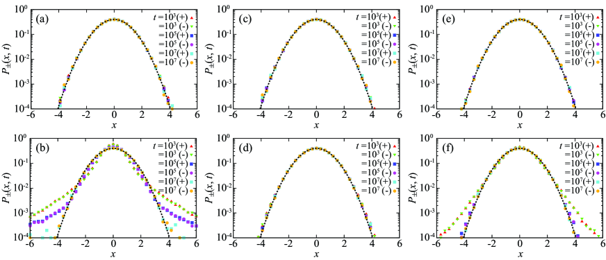
Figure 5: Non-equilibrium propagator $P_{\pm}^{\mathrm{neq}}(x,t)$ at three different times $t=10^{3},10^{5}$ and $10^{7}$ (each data is normalized so that its variance equals unity). Two non-equilibrium ensembles are used; one is started from $+$ state ($p_{+}^{0}=1$: triangle up and square), while the other from $-$ state ($p_{+}^{0}=0$: triangle down and circle). The ratio $D_{+}/D_{-}$ is set as $D_{+}/D_{-}=50$. The exponents $\alpha_{\pm}$ are set as follows: (a) [case(1-1)] $(\alpha_{+},\alpha_{-})=(0.25,0.75)$, (b) [case(1-2)] $(\alpha_{+},\alpha_{-})=(0.75,0.25)$, (c) [case(2-1)] $(\alpha_{+},\alpha_{-})=(1.25,1.75)$, (d) [case(2-2)] $(\alpha_{+},\alpha_{-})=(1.75,1.25)$, (e) [case(3-1)] $(\alpha_{+},\alpha_{-})=(0.5,1.5)$, (f) [case(3-2)] $(\alpha_{+},\alpha_{-})=(1.5,0.5)$. In (a) and (e), $P_{+}^{\mathrm{neq}}(x,t)$ is displayed; in (b) and (f), $P_{-}^{\mathrm{neq}}(x,t)$ is displayed; in (c) and (d) $P_{+}^{\mathrm{neq}}(x,t)+P_{-}^{\mathrm{neq}}(x,t)$ is displayed. The dashed lines are the Gaussian distribution with unit variance.

By using Eqs. (38) and (99), we obtain the ETMSD for the case (3-1) ($\alpha_{+}<\alpha_{-}$) as

$$\frac{\bigl{\langle}\overline{\delta\bm{r}^{2}}(\Delta;t)\bigr{\rangle}_{\mathrm{neq}}}{2n\Delta}\underset{\begin{subarray}{c}\Delta\ll t\\[0.85355pt] t\to\infty\end{subarray}}{\simeq}D_{+}-\frac{\mu_{-}}{a_{+}}\frac{(D_{+}-D_{-})t^{\alpha_{+}-1}}{\Gamma(\alpha_{+}+1)}.$$ (102)

For this case, the relaxation of the effective DC is difficult to observe, since the first term is dominant over the second all the time due to the first inequality in Eq. (88) and $D_{+}>D_{+}-D_{-}$ (i.e., there is no crossover or transient aging).

Similarly, we have the ETMSD for the case (3-2) by using Eqs. (38) and (100) as follows:

$$\frac{\bigl{\langle}\overline{\delta\bm{r}^{2}}(\Delta;t)\bigr{\rangle}_{\mathrm{neq}}}{2n\Delta}\underset{\begin{subarray}{c}\Delta\ll t\\[0.85355pt] t\to\infty\end{subarray}}{\simeq}D_{-}+\frac{\mu_{+}}{a_{-}}\frac{(D_{+}-D_{-})t^{\alpha_{-}-1}}{\Gamma(\alpha_{-}+1)}.$$ (103)

Thus, the effective DC shows a slowing down, and its exponent, $\alpha_{-}-1$, is equivalent to that of CTRW He et al. (2008). In contrast to the case (3-1), the relaxation of the effective DC can be observed, because there is a crossover between relaxation ($t^{\alpha_{-}-1}$) at short time to a plateau ($D_{-}$) at longer time; the crossover time $t_{c}$ is given by Eq. (101). That is, the system shows transient aging in this case.

The theoretical predictions for the EMSD [Eqs. (99) and (100)] and for the ETMSD [Eqs. (102) and (103)] are confirmed by numerical simulations in Fig. 4. As predicted, for $\alpha_{+}<\alpha_{-}$ [case (3-1)], the EMSD shows normal diffusion [Fig. 4(a)], whereas, for $\alpha_{-}<\alpha_{+}$ [case (3-2)], the EMSD shows transient subdiffusion [Fig. 4(b)].

VI Case study: propagator

In this section, we derive the non-equilibrium propagator, $P_{\pm}^{\mathrm{neq}}(\bm{x},t)$, at the long time limit [The equilibrium propagator, $P_{\pm}^{\mathrm{eq}}(\bm{x},t)$, is already derived in Eq. (45)]. As with the equilibrium process, the propagator has a non-Gaussian shape at short times, but in a hydrodynamic limit, it converges to Gaussian distribution if $\alpha_{+}\neq\alpha_{-}$. However, this convergence to Gaussian is very slow for the cases (1-2) and (3-2) [the slow-mode-dominated cases].

VI.1 Propagator for cases (1) and (3)

For the case (1–1) ($\alpha_{+}<\alpha_{-}$), using Eqs. (4) and (46) along with a hydrodynamic limit $s\sim\bm{k}^{2}\ll 1$, we have the leading term of the propagator

$$\breve{P}_{+}^{\mathrm{neq}}(\bm{k},s)\underset{\begin{subarray}{c}s,\bm{k}\to 0\\[-0.85355pt] s\sim\bm{k}^{2}\end{subarray}}{\simeq}\frac{1}{s+D_{+}\bm{k}^{2}},$$ (104)

and thus the propagator is Gaussian in this limit. On the other hand, $\breve{P}_{-}^{\mathrm{neq}}(\bm{k},s)$ is negligibly small compared with $\breve{P}_{+}^{\mathrm{neq}}(\bm{k},s)$. For the case (3–1), exactly the same results can be obtained. Note also that the propagator given by Eq. (104) is that of the diffusion process with a diffusion constant $D_{+}$. This is because, for these cases, the fast mode is asymptotically dominant over the slow mode as can be seen from Eq. (72), and thus long time behavior is not distinguishable from the single-mode diffusion with the diffusion constant $D_{+}$ Höfling and Franosch (2013).

Similarly, for the case (1–2) ($\alpha_{-}<\alpha_{+}$), we have the following propagator in the hydrodynamic limit:

$$\breve{P}_{-}^{\mathrm{neq}}(\bm{k},s)\underset{\begin{subarray}{c}s,\bm{k}\to 0\\[-0.85355pt] s\sim\bm{k}^{2}\end{subarray}}{\simeq}\frac{1}{s+D_{-}\bm{k}^{2}},$$ (105)

and $\breve{P}_{+}^{\mathrm{neq}}(\bm{k},s)$ is negligibly small compared with $\breve{P}_{-}^{\mathrm{neq}}(\bm{k},s)$. For the case (3–2), exactly the same results can be obtained. As expected, in these cases (1-2) and (3-2), the slow mode is asymptotically dominant over the fast one.

As shown in Fig. 5, the convergence to the Gaussian distribution for $\alpha_{-}<\alpha_{+}$ [cases (1-2) and (3-2)] is quite slow and long tails appear [Fig. 5(b) and (f)]. In contrast, for $\alpha_{+}<\alpha_{-}$ [cases (1-1) and (3-1)] the convergence is relatively fast [Fig. 5(a) and (e)].

VI.2 Propagator for case (2)

For the case (2), using Eqs. (5) and (46) along with the hydrodynamic limit $s\sim\bm{k}^{2}\ll 1$, we have the leading term of the propagator

$$\breve{P}_{\pm}^{\mathrm{neq}}(\bm{k},s)\underset{\begin{subarray}{c}s,\bm{k}\to 0\\[-0.85355pt] s\sim\bm{k}^{2}\end{subarray}}{\simeq}\frac{p_{\pm}^{\mathrm{eq}}}{s+D_{\mathrm{eq}}\bm{k}^{2}},$$ (106)

and therefore the propagator for each state, ${P}_{\pm}^{\mathrm{neq}}(\bm{x},t)$, has a Gaussian shape in the hydrodynamic limit, and the sum ${P}_{+}^{\mathrm{neq}}(\bm{x},t)+{P}_{-}^{\mathrm{neq}}(\bm{x},t)$ also becomes a Gaussian distribution. [Note that these propagators are the same as those of the equilibrium processes given in Eq. (45)]. In these cases, both fast and slow modes coexist; this is completely different behavior from the cases (1) and (3). As shown in Fig. 5(c) and (d), the convergence to the Gaussian distribution is fast in this case.

VII Case study: RSD

Here, we derive the RSD, $\Sigma(\Delta;t|\bm{w}_{0})$, for both equilibrium and non-equilibrium processes, and show that it exhibits slow relaxation as a consequence of the fluctuating diffusivity (except for some parameter ranges in which the RSD shows normal relaxation). As shown in the previous sections, for the cases (1-2) and (3-2), the EMSD and ETMSD exhibit anomalous behaviors such as the transient subdiffusion and transient aging. In contrast, for the other cases including equilibrium processes, both EMSD and ETMSD show normal diffusion and they do not exhibit (or it is difficult to observe) any anomalous behaviors. Therefore, for these cases, we can not find any traces of the fluctuating diffusivity with these MSDs. To find the anomaly of diffusivity, we have to study higher order moments such as the RSD.

VII.1 Equilibrium RSD

Figure 6: Equilibrium RSD $\Sigma(\Delta;t|\bm{w}^{\mathrm{eq}})$ vs total measurement time $t$ for the case (2). The exponents $\alpha_{\pm}$ are set as follows: $(\alpha_{+},\alpha_{-})=(1.25,1.75)$ [case(2–1): triangle up] and $(\alpha_{+},\alpha_{-})=(1.75,1.25)$ [case(2–2): square]. The lag time $\Delta$ is set as $\Delta=0.1$. The lines are the theoretical prediction [Eqs. (110) and (112)]. There are no fitting parameters (The same is true of Figs. 7 and 8).

First, we consider the equilibrium ACF $\langle\delta D(t)\delta D(0)\rangle_{\mathrm{eq}}$ by using Eq. (66). We study only the case (2), since the other cases does not have equilibrium states. With Eqs. (5) and (17), the transition probabilities for $\alpha_{+}<\alpha_{-}$ [case (2-1)] are found to be

$$\begin{split}\hat{W}_{\pm\pm}^{\mathrm{eq}}(s)&\underset{s\to 0}{\simeq}\frac{\left(p_{\pm}^{\mathrm{eq}}\right)^{2}}{s}+\frac{a_{+}\left(p_{-}^{\mathrm{eq}}\right)^{2}}{\mu s^{2-\alpha_{+}}},\\[0.0pt] \hat{W}_{\pm\mp}^{\mathrm{eq}}(s)&\underset{s\to 0}{\simeq}\frac{p_{+}^{\mathrm{eq}}p_{-}^{\mathrm{eq}}}{s}-\frac{a_{+}\left(p_{-}^{\mathrm{eq}}\right)^{2}}{\mu s^{2-\alpha_{+}}}.\end{split}$$ (107)

Then, from Eq. (66), the ACF is given by

$$\left\langle\delta\hat{D}(s)\delta D(0)\right\rangle_{\mathrm{eq}}\underset{s\to 0}{\simeq}(D_{+}-D_{-})^{2}\frac{a_{+}(p_{-}^{\mathrm{eq}})^{2}}{\mu s^{2-\alpha_{+}}},$$ (108)

and the Laplace inversion becomes

$$\left\langle\delta D(t)\delta D(0)\right\rangle_{\mathrm{eq}}\underset{t\to\infty}{\simeq}\frac{(D_{+}-D_{-})^{2}(p_{-}^{\mathrm{eq}})^{2}}{\Gamma(2-\alpha_{+})}\frac{a_{+}}{\mu}t^{1-\alpha_{+}}.$$ (109)

Thus, in contrast to the MSDs which behave normally, the ACF show slow relaxation. By using Eqs. (61) and (108), we obtain the RSD

$$\Sigma^{2}(\Delta;t|\bm{w}^{\mathrm{eq}})\underset{t\to\infty}{\approx}\frac{2(D_{+}-D_{-})^{2}(p_{-}^{\mathrm{eq}})^{2}}{D_{\mathrm{eq}}^{2}\Gamma(4-\alpha_{+})}\frac{a_{+}}{\mu}t^{1-\alpha_{+}},$$ (110)

where we used $\Sigma^{2}(\Delta;t|\bm{w}^{\mathrm{eq}})\approx\Sigma^{2}_{\mathrm{ex}}(t|\bm{w}^{\mathrm{eq}})$, because the ideal RSD, $\Sigma^{2}_{\mathrm{id}}(\Delta;t|\bm{w}^{\mathrm{eq}})$, decays faster than $\Sigma^{2}_{\mathrm{ex}}(t|\bm{w}^{\mathrm{eq}})$ (see the last paragraph of Sec. III.6). The same asymptotic approximation is used repeatedly in the following subsections.

The ACF shows slow relaxation also for $\alpha_{-}<\alpha_{+}$ [case(2-2)] as

$$\!\left\langle\delta D(t)\delta D(0)\right\rangle_{\mathrm{eq}}\underset{t\to\infty}{\simeq}\frac{(D_{+}-D_{-})^{2}(p_{+}^{\mathrm{eq}})^{2}}{\Gamma(2-\alpha_{-})}\frac{a_{-}}{\mu}t^{1-\alpha_{-}}.\!$$ (111)

This equation can be obtained by using Eqs. (5) and (17), or more simply, by substituting $\pm$ signs of subscripts in Eq. (109) for $\mp$ signs. Also, we have the RSD

$$\Sigma^{2}(\Delta;t|\bm{w}^{\mathrm{eq}})\underset{t\to\infty}{\approx}\frac{2(D_{+}-D_{-})^{2}(p_{+}^{\mathrm{eq}})^{2}}{D_{\mathrm{eq}}^{2}\Gamma(4-\alpha_{-})}\frac{a_{-}}{\mu}t^{1-\alpha_{-}}.$$ (112)

Thus, in these cases, the RSD, $\Sigma(\Delta;t|\bm{w}^{\mathrm{eq}})$, decays slower than $t^{-1/2}$; this is the same behavior as the CTRW with the power-law exponent $\alpha\in(1,2)$ of the waiting time PDF Akimoto et al. (2011).

Note also that Eqs. (110) and (112) are valid for $\Delta$ smaller than the characteristic correlation time of $D(t)$ [This is the assumption used in the derivation of Eq. (53)]. We show results of numerical simulations for the cases (2-1) and (2-2) in Fig. 6. These results are found to be consistent with the theoretical predictions.

VII.2 Non-equilibrium RSD for case (1)

To derive expressions for the non-equilibrium RSD, we start with the estimate of $\delta\breve{W}_{hh^{\prime}}^{\mathrm{neq}}(s_{1},s_{2})$, because the excess RSD, $\Sigma_{\mathrm{ex}}(t_{1},t_{2}|\bm{w}^{\mathrm{neq}})$, is obtained from the ACF $\langle\delta\hat{D}(s_{1})\delta\hat{D}(s_{2})\rangle_{\mathrm{neq}}$ [Eq. (III.6.2)], which in turn can be expressed with $\delta\breve{W}_{hh^{\prime}}^{\mathrm{neq}}(s_{1},s_{2})$ [Eq. (70)]. For $\alpha_{+}<\alpha_{-}$ [case (1-1)], from Eqs. (4), (69), (71), (149), (156), we obtain

$$\begin{split}\!\!\delta\breve{W}_{\pm\pm}^{\mathrm{neq}}(s_{1},s_{2})\!&\underset{\begin{subarray}{c}s_{1},s_{2}\to 0\\[0.0pt] s_{1}\sim s_{2}\end{subarray}}{\simeq}\frac{a_{-}}{a_{+}}\frac{s_{1}^{\alpha_{-}}+s_{2}^{\alpha_{-}}-(s_{1}+s_{2})^{\alpha_{-}}}{s_{1}s_{2}(s_{1}+s_{2})^{\alpha_{+}}},\!\!\\[0.0pt] \!\!\delta\breve{W}_{\pm\mp}^{\mathrm{neq}}(s_{1},s_{2})\!&\underset{\begin{subarray}{c}s_{1},s_{2}\to 0\\[0.0pt] s_{1}\sim s_{2}\end{subarray}}{\simeq}\frac{a_{-}}{a_{+}}\frac{(s_{1}+s_{2})^{\alpha_{-}}-s_{1}^{\alpha_{-}}-s_{2}^{\alpha_{-}}}{s_{1}s_{2}(s_{1}+s_{2})^{\alpha_{+}}},\!\!\end{split}$$ (113)

where we assume that $s_{1}$ and $s_{2}$ are comparable ($s_{1}\sim s_{2}$). In deriving the above equation for $\delta\breve{W}_{-+}(s_{1},s_{2})$, we used the relation $\delta\breve{W}_{-+}(s_{1},s_{2})=\delta\breve{W}_{+-}(s_{2},s_{1})$, which is easily checked by Eqs. (69), (149) and (156). From Eq. (70), we obtain

$$\frac{\langle\delta\hat{D}(s_{1})\delta\hat{D}(s_{2})\rangle_{\mathrm{neq}}}{s_{1}s_{2}} \underset{\begin{subarray}{c}s_{1},s_{2}\to 0\\[-0.85355pt] s_{1}\sim s_{2}\end{subarray}}{\simeq}$$

$$(D_{+}-D_{-})^{2} \frac{a_{-}}{a_{+}}\frac{s_{1}^{\alpha_{-}}+s_{2}^{\alpha_{-}}-(s_{1}+s_{2})^{\alpha_{-}}}{s_{1}^{2}s_{2}^{2}(s_{1}+s_{2})^{\alpha_{+}}},$$ (114)

Setting $t_{1}=t_{2}=t$ in the double Laplace inversions of Eq. (VII.2) (see Appendix D), we obtain from Eqs. (III.6.2) and (89)

$$\Sigma^{2}(\Delta;t|\bm{w}^{\mathrm{neq}})\underset{\begin{subarray}{c}\Delta\ll t\\[0.85355pt] t\to\infty\end{subarray}}{\approx}\left(\frac{D_{+}-D_{-}}{D_{+}}\right)^{2}\frac{a_{-}}{a_{+}}\frac{2(1-\alpha_{-})\,t^{\alpha_{+}-\alpha_{-}}}{\Gamma(3+\alpha_{+}-\alpha_{-})},$$ (115)

for $\alpha_{+}<\alpha_{-}$ [case (1-1)].

On the other hand, we obtain the RSD for $\alpha_{-}<\alpha_{+}$ [case (1-2)], by substituting $\pm$ signs of the subscripts in Eq. (115) for $\mp$ signs,

$$\Sigma^{2}(\Delta;t|\bm{w}^{\mathrm{neq}})\underset{\begin{subarray}{c}\Delta\ll t\\[0.85355pt] t\to\infty\end{subarray}}{\approx}\left(\frac{D_{+}-D_{-}}{D_{-}}\right)^{2}\frac{a_{+}}{a_{-}}\frac{2(1-\alpha_{+})t^{\alpha_{-}-\alpha_{+}}}{\Gamma(3+\alpha_{-}-\alpha_{+})},$$ (116)

As with the equilibrium RSD, Eqs. (115) and (116) are valid for $\Delta$ shorter than the characteristic correlation time of $D(t)$ [The same is true of the results for the cases (2) and (3) in the following subsections].

In Fig. 7 (a) and (b), numerical simulations of the RSD are displayed for the cases (1-1) and (1-2), respectively. Apparently, the RSD for the case (1-2) decays slower than that for the case (1-1). This is consistent with the slow convergence to the Gaussian distribution observed in Fig. 5 (b); note that the excess RSD is equivalent to a non-Gaussian parameter (see Appendix E).

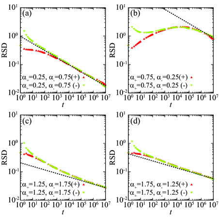
Figure 7: Non-equilibrium RSD $\Sigma(\Delta;t|\bm{w}^{\mathrm{neq}})$ vs total measurement time $t$ for the cases (1) and (2). $\alpha_{\pm}$ are set as follows: (a) [case(1–1)] $(\alpha_{+},\alpha_{-})=(0.25,0.75)$, (b) [case(1–2)] $(\alpha_{+},\alpha_{-})=(0.75,0.25)$, (c) [case(2–1)] $(\alpha_{+},\alpha_{-})=(1.25,1.75)$, and (d) [case(2–2)] $(\alpha_{+},\alpha_{-})=(1.75,1.25)$. For all the figures, $\Delta$ is set as $\Delta=0.1$, and results for ensembles starting from $+$ state (triangles up) and $-$ state (triangles down) are displayed. The lines in (a), (b), (c), and (d) are theoretical predictions given in Eqs. (115) (116), (119), and (120), respectively.

VII.3 Non-equilibrium RSD for case (2)

For $\alpha_{+}<\alpha_{-}$ [case (2-1)], from Eqs. (5), (69), (79), (149), (156), we obtain (after a lengthy calculation)

$$\begin{split}\delta\breve{W}_{\pm\pm}^{\mathrm{neq}}(s_{1},s_{2})&\underset{\begin{subarray}{c}s_{1},s_{2}\to 0\\[0.0pt] s_{1}\sim s_{2}\end{subarray}}{\simeq}\frac{a_{+}(p_{-}^{\mathrm{eq}})^{2}}{\mu}\frac{(s_{1}+s_{2})^{\alpha_{+}}-s_{1}^{\alpha_{+}}-s_{2}^{\alpha_{+}}}{s_{1}s_{2}(s_{1}+s_{2})},\\[0.0pt] \delta\breve{W}_{\pm\mp}^{\mathrm{neq}}(s_{1},s_{2})&\underset{\begin{subarray}{c}s_{1},s_{2}\to 0\\[0.0pt] s_{1}\sim s_{2}\end{subarray}}{\simeq}\frac{a_{+}(p_{-}^{\mathrm{eq}})^{2}}{\mu}\frac{s_{1}^{\alpha_{+}}+s_{2}^{\alpha_{+}}-(s_{1}+s_{2})^{\alpha_{+}}}{s_{1}s_{2}(s_{1}+s_{2})},\end{split}$$ (117)

where we assume that $s_{1}$ and $s_{2}$ are comparable (i.e., $s_{1}\sim s_{2}$). Thus, from Eq. (70), we obtain

$$\frac{\langle\delta\hat{D}(s_{1})\delta\hat{D}(s_{2})\rangle_{\mathrm{neq}}}{s_{1}s_{2}} \underset{\begin{subarray}{c}s_{1},s_{2}\to 0\\[0.0pt] s_{1}\sim s_{2}\end{subarray}}{\simeq}$$ (118)

$$\frac{a_{+}(p_{-}^{\mathrm{eq}})^{2}(D_{+}-D_{-})^{2}}{\mu}\frac{(s_{1}+s_{2})^{\alpha_{+}}-s_{1}^{\alpha_{+}}-s_{2}^{\alpha_{+}}}{s_{1}^{2}s_{2}^{2}(s_{1}+s_{2})},$$

Setting $t_{1}=t_{2}=t$ in the double Laplace inversions of Eq. (118), we obtain from Eqs. (III.6.2) and (94)

$$\Sigma^{2}(\Delta;t|\bm{w}^{\mathrm{neq}})\underset{\begin{subarray}{c}\Delta\ll t\\[0.85355pt] t\to\infty\end{subarray}}{\approx}\frac{2(\alpha_{+}-1)(D_{+}-D_{-})^{2}(p_{-}^{\mathrm{eq}})^{2}}{D_{\mathrm{eq}}^{2}\Gamma(4-\alpha_{+})}\frac{a_{+}}{\mu}t^{1-\alpha_{+}},$$ (119)

for $\alpha_{+}<\alpha_{-}$ [case (2-1)]. On the other hand, by substituting $\pm$ signs of subscripts in Eq. (119) for $\mp$ sign, we obtain the RSD for $\alpha_{-}<\alpha_{+}$ [case (2-2)] as

$$\Sigma^{2}(\Delta;t|\bm{w}^{\mathrm{neq}})\underset{\begin{subarray}{c}\Delta\ll t\\[0.85355pt] t\to\infty\end{subarray}}{\approx}\frac{2(\alpha_{-}-1)(D_{+}-D_{-})^{2}(p_{+}^{\mathrm{eq}})^{2}}{D_{\mathrm{eq}}^{2}\Gamma(4-\alpha_{-})}\frac{a_{-}}{\mu}t^{1-\alpha_{-}}.$$ (120)

Note that the asymptotic scalings $\left(t^{1-\alpha_{\pm}}\right)$ of Eqs. (119) and (120) are the same as those of the equilibrium case [Eqs. (110) and (112)]. But there are slight differences in prefactors; i.e., the non-equilibrium RSDs are smaller than the equilibrium ones.

VII.4 Non-equilibrium RSD for case (3): $\alpha_{+}+\alpha_{-}<2$

For the case (3), the RSD behaves differently depending whether $\alpha_{+}+\alpha_{-}<2$ or $\alpha_{+}+\alpha_{-}>2$. Let us begin with the case of $\alpha_{+}+\alpha_{-}<2$. For the case (3-1) $(\alpha_{+}<\alpha_{-})$, we obtain results similar to the case (1) [Eqs. (113)– (116)] as follows:

$$\begin{split}\!\!\!\delta\breve{W}_{\pm\pm}^{\mathrm{neq}}(s_{1},s_{2})\!&\underset{\begin{subarray}{c}s_{1},s_{2}\to 0\\[0.0pt] s_{1}\sim s_{2}\end{subarray}}{\simeq}\frac{a_{-}}{a_{+}}\frac{(s_{1}+s_{2})^{\alpha_{-}}-s_{1}^{\alpha_{-}}-s_{2}^{\alpha_{-}}}{s_{1}s_{2}(s_{1}+s_{2})^{\alpha_{+}}},\!\\[0.0pt] \!\!\!\delta\breve{W}_{\pm\mp}^{\mathrm{neq}}(s_{1},s_{2})\!&\underset{\begin{subarray}{c}s_{1},s_{2}\to 0\\[0.0pt] s_{1}\sim s_{2}\end{subarray}}{\simeq}\frac{a_{-}}{a_{+}}\frac{s_{1}^{\alpha_{-}}+s_{2}^{\alpha_{-}}-(s_{1}+s_{2})^{\alpha_{-}}}{s_{1}s_{2}(s_{1}+s_{2})^{\alpha_{+}}},\!\end{split}$$ (121)

where we used Eqs. (4), (5), (69), (84), (85), (149), and (156) Note (2). These equations are almost the same as Eq. (113) except for their signs. Thus, the RSD is obtained by changing the sign of Eq. (115) as

$$\Sigma^{2}_{\mathrm{ex}}(t|\bm{w}^{\mathrm{neq}})\underset{\begin{subarray}{c}t\to\infty\end{subarray}}{\simeq}\left(\frac{D_{+}-D_{-}}{D_{+}}\right)^{2}\frac{a_{-}}{a_{+}}\frac{2(\alpha_{-}-1)\,t^{\alpha_{+}-\alpha_{-}}}{\Gamma(3+\alpha_{+}-\alpha_{-})},$$ (122)

for $\alpha_{+}<\alpha_{-}$ [case(3-1)]. Note that $\Sigma^{2}_{\mathrm{ex}}(t|\bm{w}^{\mathrm{neq}})$ decays faster than $O(1/t)$, if $\alpha_{-}-\alpha_{+}>1$. In such a case, the ideal RSD, $\Sigma^{2}_{\mathrm{id}}(\Delta;t|\bm{w}^{\mathrm{neq}})$ [Eq. (58)], which is of the order of $O(1/t)$, becomes the dominant term, and the excess RSD, $\Sigma^{2}_{\mathrm{ex}}(t|\bm{w}^{\mathrm{neq}})$ [Eqs. (122)], becomes the second leading term:

$$\Sigma^{2}(\Delta;t|\bm{w}^{\mathrm{neq}})\underset{\begin{subarray}{c}\Delta\ll t\\[0.85355pt] t\to\infty\end{subarray}}{\approx}\frac{4\Delta}{3nt}+\Sigma^{2}_{\mathrm{ex}}(t|\bm{w}^{\mathrm{neq}}).$$ (123)

In contrast, if $\alpha_{-}-\alpha_{+}<1$, $\Sigma^{2}_{\mathrm{ex}}(t|\bm{w}^{\mathrm{neq}})$ decays slower than $O(1/t)$, and thus this is the dominant term:

$$\Sigma^{2}(\Delta;t|\bm{w}^{\mathrm{neq}})\underset{\begin{subarray}{c}\Delta\ll t\\[0.85355pt] t\to\infty\end{subarray}}{\approx}\Sigma^{2}_{\mathrm{ex}}(t|\bm{w}^{\mathrm{neq}}).$$ (124)

As shown in Fig. 8(a), results of numerical simulations are consistent with these asymptotic behaviors.

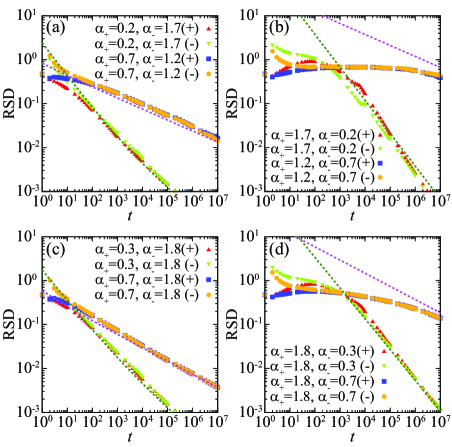
Figure 8: Non-equilibrium RSD $\Sigma(\Delta;t|\bm{w}^{\mathrm{neq}})$ vs total measurement time $t$ for the cases (3-1) and (3-2). $\alpha_{\pm}$ are set as follows: (a) [case(3-1) with $\alpha_{+}+\alpha_{-}<2$] $(\alpha_{+},\alpha_{-})=(0.2,1.7)$ and $(0.7,1.2)$, (b) [case(3-2) with $\alpha_{+}+\alpha_{-}<2$] $(\alpha_{+},\alpha_{-})=(1.7,0.2)$ and $(1.2,0.7)$ (c) [case(3-1) with $\alpha_{+}+\alpha_{-}>2$] $(\alpha_{+},\alpha_{-})=(0.3,1.8)$ and $(0.7,1.8)$, and (d) [case(3-2) with $\alpha_{+}+\alpha_{-}>2$] $(\alpha_{+},\alpha_{-})=(1.8,0.3)$ and $(1.8,0.7)$. For all the figures, $\Delta$ is set as $\Delta=0.1$, and results for ensembles starting from $+$ state (triangles up and squares) and $-$ state (triangles down and circles) are displayed. The pink lines in (a), (b), (c), and (d) are theoretical predictions for $\Sigma_{\mathrm{ex}}(t|\bm{w}^{\mathrm{neq}})$ given by Eqs. (122), (125), (128), and (129), respectively. Each green line is $[4\Delta/(3nt)+\Sigma_{\mathrm{ex}}^{2}(t|\bm{w}^{\mathrm{neq}})]^{1/2}$ [Eq. (123)], in which $\Sigma_{\mathrm{ex}}(t|\bm{w}^{\mathrm{neq}})$ is the same as the pink line.

On the other hand, we obtain the RSD for the case (3-2) $(\alpha_{-}<\alpha_{+})$ by replacing $\pm$ signs of subscripts in Eq. (122) with $\mp$ signs:

$$\Sigma^{2}_{\mathrm{ex}}(t|\bm{w}^{\mathrm{neq}})\underset{\begin{subarray}{c}t\to\infty\end{subarray}}{\simeq}\left(\frac{D_{+}-D_{-}}{D_{-}}\right)^{2}\frac{a_{+}}{a_{-}}\frac{2(\alpha_{+}-1)\,t^{\alpha_{-}-\alpha_{+}}}{\Gamma(3+\alpha_{-}-\alpha_{+})}.$$ (125)

As with the case (3-1), $\Sigma^{2}_{\mathrm{ex}}(t|\bm{w}^{\mathrm{neq}})$ decays faster than $O(1/t)$, if $\alpha_{+}-\alpha_{-}>1$. Then, the dominant term is given by $\Sigma^{2}_{\mathrm{id}}(\Delta;t|\bm{w}^{\mathrm{neq}})$ in Eq. (58), and thus the asymptotic RSD is again reduced to Eq. (123) in which $\Sigma^{2}_{\mathrm{ex}}(t|\bm{w}^{\mathrm{neq}})$ is given by Eq. (125). Contrastingly, if $\alpha_{+}-\alpha_{-}<1$, $\Sigma^{2}_{\mathrm{ex}}(t|\bm{w}^{\mathrm{neq}})$ decays slower than $O(1/t)$, and thus this term is dominant. Accordingly, the RSD behaves as Eq. (124) in which $\Sigma^{2}_{\mathrm{ex}}(t|\bm{w}^{\mathrm{neq}})$ is given by Eq. (125). As shown in Fig. 8 (b), we found good agreements between these theories and numerical results. In particular, when $\alpha_{+}-\alpha_{-}<1$, the RSD decays quite slowly.

VII.5 Non-equilibrium RSD for case (3): $\alpha_{+}+\alpha_{-}>2$

Now we study the case in which $\alpha_{+}+\alpha_{-}>2$. Let us start with the case (3-1) $(\alpha_{+}<\alpha_{-})$. We obtain the following expressions for $\delta\breve{W}_{\pm\pm}^{\mathrm{neq}}(s_{1},s_{2})$ and $\delta\breve{W}_{\pm\mp}^{\mathrm{neq}}(s_{1},s_{2})$ from Eqs. (4), (5), (69), (84), (85), (149), and (156) Note (2):

$$\begin{split}\delta\breve{W}_{\pm\pm}^{\mathrm{neq}}(s_{1},s_{2})&\underset{\begin{subarray}{c}s_{1},s_{2}\to 0\\[0.0pt] s_{1}\sim s_{2}\end{subarray}}{\simeq}\left(\frac{\mu_{-}}{a_{+}}\right)^{2}\frac{s_{1}^{\alpha_{+}}+s_{2}^{\alpha_{+}}-(s_{1}+s_{2})^{\alpha_{+}}}{[s_{1}s_{2}(s_{1}+s_{2})]^{\alpha_{+}}},\\[0.0pt] \delta\breve{W}_{\pm\mp}^{\mathrm{neq}}(s_{1},s_{2})&\underset{\begin{subarray}{c}s_{1},s_{2}\to 0\\[0.0pt] s_{1}\sim s_{2}\end{subarray}}{\simeq}\left(\frac{\mu_{-}}{a_{+}}\right)^{2}\frac{(s_{1}+s_{2})^{\alpha_{+}}-s_{1}^{\alpha_{+}}-s_{2}^{\alpha_{+}}}{[s_{1}s_{2}(s_{1}+s_{2})]^{\alpha_{+}}},\end{split}$$ (126)

where we assume that $s_{1}$ and $s_{2}$ are comparable (i.e., $s_{1}\sim s_{2}$). Thus, from Eq. (70), we obtain

$$\frac{\langle\delta\hat{D}(s_{1})\delta\hat{D}(s_{2})\rangle_{\mathrm{neq}}}{s_{1}s_{2}} \underset{\begin{subarray}{c}s_{1},s_{2}\to 0\\[0.0pt] s_{1}\sim s_{2}\end{subarray}}{\simeq}(D_{+}-D_{-})^{2}\left(\frac{\mu_{-}}{a_{+}}\right)^{2}$$

$$\times\frac{s_{1}^{\alpha_{+}}+s_{2}^{\alpha_{+}}-(s_{1}+s_{2})^{\alpha_{+}}}{(s_{1}s_{2})^{\alpha_{+}+1}(s_{1}+s_{2})^{\alpha_{+}}}.$$ (127)

Setting $t_{1}=t_{2}=t$ in the double Laplace inversions of this equation, we obtain from Eqs. (III.6.2) and (99)

$$\Sigma^{2}_{\mathrm{ex}}(t|\bm{w}^{\mathrm{neq}}) \underset{\begin{subarray}{c}t\to\infty\end{subarray}}{\simeq}\left(\frac{D_{+}-D_{-}}{D_{+}}\right)^{2}\left(\frac{\mu_{-}}{a_{+}}\right)^{2}$$

$$\times \frac{t^{2\alpha_{+}-2}}{\Gamma^{2}(\alpha_{+}+1)}\left[\frac{2\Gamma^{2}(\alpha_{+}+1)}{\Gamma(2\alpha_{+}+1)}-1\right],$$ (128)

for $\alpha_{+}<\alpha_{-}$ [case (3-1)]. Note that, if $\alpha_{+}<1/2$, $\Sigma^{2}_{\mathrm{ex}}(t|\bm{w}^{\mathrm{neq}})$ decays faster than $O(1/t)$. Therefore, the ideal RSD $\Sigma^{2}_{\mathrm{id}}(\Delta;t|\bm{w}^{\mathrm{neq}})$ given by Eq. (58) becomes the dominant term, and the excess part $\Sigma^{2}_{\mathrm{ex}}(t|\bm{w}^{\mathrm{neq}})$ [Eq. (128)] is the second leading contribution. In this case (i.e., $\alpha_{+}<1/2$), the RSD asymptotically behaves as Eq. (123) in which $\Sigma^{2}_{\mathrm{ex}}(t|\bm{w}^{\mathrm{neq}})$ is given by Eq. (128).

Moreover, the RSD for the case (3-2) $\left(\alpha_{-}<\alpha_{+}\right)$ is obtained by replacing $\pm$ signs of the subscripts in Eq. (128) with $\mp$ signs:

$$\Sigma^{2}_{\mathrm{ex}}(t|\bm{w}^{\mathrm{neq}}) \underset{\begin{subarray}{c}t\to\infty\end{subarray}}{\simeq}\left(\frac{D_{+}-D_{-}}{D_{-}}\right)^{2}\left(\frac{\mu_{+}}{a_{-}}\right)^{2}$$

$$\times \frac{t^{2\alpha_{-}-2}}{\Gamma^{2}(\alpha_{-}+1)}\left[\frac{2\Gamma^{2}(\alpha_{-}+1)}{\Gamma(2\alpha_{-}+1)}-1\right].$$ (129)

Again, the leading term is switched at $\alpha_{-}=1/2$ from $\Sigma^{2}_{\mathrm{id}}(\Delta;t|\bm{w}^{\mathrm{neq}})$ to $\Sigma^{2}_{\mathrm{ex}}(t|\bm{w}^{\mathrm{neq}})$. As shown in Fig. 8(c) and (d), we checked these asymptotic behaviors by numerical simulations, and found good agreements with these theory. The asymptotic scaling behavior of the non-equilibrium RSD is summarized in Fig. 9, which shows that the RSD exhibits slow relaxation $O(1/t^{\beta})$ with $\beta<1$ for most of the parameter values $(\alpha_{+},\alpha_{-})$; the exceptions are some parameter domains inside of the cases (3-1) and (3-2), in which the RSD decays as $O(1/t)$.

Figure 9: Phase diagram for asymptotic behaviors of the non-equilibrium RSD, $\Sigma^{2}(\Delta;t|\bm{w}^{\mathrm{neq}})$, on the $\alpha_{+}\alpha_{-}$ plane. The solid lines represent boundaries dividing the six cases (1-1), (1-2), (2-1), (2-2), (3-1), and (3-2). The dashed lines are boundaries dividing the cases (3-1) and (3-2) into subclasses according to the scaling behavior of the RSD.

VIII Discussion

VIII.1 Summary

In many biological experiments Golding and Cox (2006); Burov et al. (2011); Jeon et al. (2011); Weigel et al. (2011) and molecular dynamics simulations Akimoto et al. (2011); Yamamoto et al. (2014, 2015), scatter of DCs has been reported. To model such scatter, CTRW and related models have been studied extensively, and it is found that these models exhibit distributional ergodicity—namely, the DC behaves as a random variable He et al. (2008); Neusius et al. (2009); Meroz et al. (2010); Miyaguchi and Akimoto (2011, 2013). This phenomenon is reminiscent of the scatter of DC observed in experiments. Some experimental studies, however, show that the DC temporally fluctuates between two distinct values Yamamoto and Onuki (1998a, b); Knight and Falke (2009); Leith et al. (2012); Parry et al. (2014). The CTRW type models should not be suitable as a model of such dichotomous fluctuations of the DC, since these models do not consist of two diffusion modes, but of long quiescent states and instantaneous jumps.

In this paper, we studied a Langevin equation with two diffusion modes (fast and slow diffusion modes) for equilibrium and non-equilibrium ensembles. We found that the EMSD shows normal diffusion or transient subdiffusion depending on the sojourn time PDFs, and that the TMSD shows only normal diffusion. Thus, it is impossible with the TMSD to find a trace of fluctuating diffusivity. This is a serious problem, since, in many experiments, the TMSD is frequently utilized to calculate the MSD. As an alternative approach, we have proposed the RSD analysis with which we can extract information of the ACF, $\left\langle D(t_{1})D(t_{2})\right\rangle$, from trajectory data $\bm{x}(t)$ [namely, the instantaneous DC, $D(t)$, is not necessary to measure directly]. It is also worth noting that the excess RSD is equivalent to a non-Gaussian parameter. From these facts, the RSD analysis should be a very useful tool to analyze the fluctuating diffusivity in single-particle-tracking experiments. In the case studies for the power-law sojourn time PDFs, we also show that the RSD decays slower than $t^{-1/2}$. Such slow relaxation in RSD is observed in molecular dynamics simulations for the center-of-mass motion of a lipid molecule in a lipid bilayer Akimoto et al. (2011).

We also show that the propagator has a non-Gaussian shape for short time, and converges to the Gaussian distribution asymptotically. This convergence to Gaussian is extremely slow for the cases in which the slow mode dominates over the fast one [cases (1-2) and (3-2)]. Furthermore, in these slow-mode-dominated cases, the EMSD shows transient subdiffusion, and the effective DC of the ETMSD exhibits transient aging. On the other hand, the equilibrium processes show the short-time non-Gaussianity, and yet normal diffusion in both EMSD and ETMSD. This is consistent with the findings reported in Chubynsky and Slater (2014), in which a random walk model with fluctuating diffusivity is studied.

In addition, if we take a limit $D_{-}\to 0$ in the slow-mode-dominated cases [cases (1-2) and (3-2)], the behaviors of the system become very similar to those of CTRW. In fact, the crossover time from the transient to asymptotic regimes, $t_{c}$ [Eqs. (91) and (101)], diverges when $D_{-}\to 0$, thereby permanent subdiffusion and aging are observed. This implies that the scatter of the DC reported in many single-particle-tracking experiments Golding and Cox (2006); Burov et al. (2011); Jeon et al. (2011) and molecular dynamics simulations Akimoto et al. (2011); Yamamoto et al. (2014, 2015), which so far has been attributed to CTRW dynamics, may well be originated from the fluctuating diffusivity. Moreover, although we studied the LEFD with dichotomous DCs, some of the general results presented in Sec. III are valid for a general LEFD. In fact, Eqs. (24), (37) and (53) are valid for arbitrary stochastic processes $D(t)$.

Also, we confirmed our theoretical results by extensive numerical simulations. Importantly, we used an experimentally plausible ratio between the two DCs, $D_{+}/D_{-}=50$ (see Parry et al. (2014), in which diffusion in the bacterial cells is studied. See also Appendix F), and observed singular behaviors such as the transient subdiffusion, non-Gaussianity of the propagator, and slow relaxation in the RSD. This means that these singular behaviors might be measurable also in single-particle-tracking experiments of bacterial cells.

VIII.2 Outlook

Mechanisms of fluctuating diffusivity observed in crowded and glass-like systems are still unclear Yamamoto and Onuki (1998a, b); Parry et al. (2014) (except for the reptation dynamics in which fluctuating diffusivity originates from the the end-to-end vector fluctuations Uneyama et al. (2015)). Usually, tagged-particle diffusion can be described by a generalized Langevin equation (GLE). When deriving the GLE with the projection operator method Mori (1955), however, we have to assume a separation of time scales of the tagged particle (slow variables) and environment (fast variables). Thus, the fluctuating diffusivity might be due to a violation of this separation of the time scales.

It is also worth mentioning the GLE and fractional Brownian motion (FBM) Deng and Barkai (2009); Ferreira et al. (2012). The main difference between these systems and the LEFD is in that the GLE and FBM have Gaussian propagators since they are Gaussian processes, whereas the LEFD shows non-Gaussian behavior (Though, some recent works studied GLEs with the Lévy stable noise, which shows non-Gaussianity Srokowski (2013)). Moreover, for the GLE and FBM, the velocity ACF exhibits power law decay Pottier (2003), while that of the LEFD is delta-correlated

$$\left\langle\bm{v}(t)\bm{v}(t^{\prime})\right\rangle=2n\left\langle D(t)\right\rangle\delta(t-t^{\prime}).$$ (130)

In this sense, both GLE/FMB and LEFD are extreme models, and real systems might show both properties: non-Gaussianity and slow decay of the velocity ACF.

As presented in Parry et al. (2014), relatively large particles in bacterial cells with a normal metabolism show fast and slow diffusion modes, which motivates us to study the LEFD with the dichotomous DCs. On the other hand, in metabolically dormant cells, this dichotomy of the DC almost vanishes and a single peak at zero-diffusivity appears in the PDF of the diffusivity (Fig.5B in Parry et al. (2014)). To describe this type of behavior, other models such as the ATTM Massignan et al. (2014); Manzo et al. (2015) would be important. Moreover, the TMSD measured in Parry et al. (2014) shows subdiffusion, while the TMSD of the LEFD only shows normal diffusion. This discrepancy would be explained by considering a finite size (confinement) effect He et al. (2008); Neusius et al. (2009); Miyaguchi and Akimoto (2013).

In this article, we only studied some basic properties of the LEFD such as the MSDs and propagators, but more advanced properties such as the first passage time, escape statistics, diffusion on potentials landscapes are also interesting subjects to study. In particular, the first passage time is important in the analysis of intermittent search problems Loverdo et al. (2009); Bénichou et al. (2011). In earlier studies Reingruber and Holcman (2009, 2010), the Markovian switching between fast and slow diffusion modes is investigated as an efficient search strategy, but effects of non-Markovian switchings on the search efficiency may be important. To understand such non-Markovian effects, the two-state renewal theory developed in this article is essential. This two-state renewal theory will also be utilized in various fields of science, since many natural systems behave like two-state systems (e.g., ion-channel gating Goychuk and Hänggi (2003), blinking quantum dots Kuno et al. (2000); Brokmann et al. (2003), and Kardar-Parisi-Zhang fluctuations Takeuchi and Akimoto (2015)).

In addition, we concentrated on the equilibrium and a typical non-equilibrium ensembles, and did not analyze aging processes which is assumed to start at $t=-t_{a}$ Barkai and Cheng (2003); Schulz et al. (2014). However, the aging phenomena can be analyzed to some extent by using the general transition probabilities given in Eq. (156), or more simply by replacing the initial ensemble $\bm{w}^{0}(\tau)=\{w^{0}_{\pm}(\tau)\}$ with the the forward recurrence time PDF $\bm{w}_{a}^{\mathrm{neq}}(\tau):=\{w_{\pm}^{\mathrm{neq}}(\tau;t_{a})\}$ [Eq. (148)] in various results. For example, $p_{\pm}(t|\bm{w}_{a}^{\mathrm{neq}})$ is the fractions at $t$ for a process that started at $t=-t_{a}$ with the initial ensemble $\bm{w}^{\mathrm{neq}}(\tau)$.

Appendix A Another derivation of $\hat{Q}_{\pm,n}(s)$

In Sec. III, we derive $\hat{Q}_{\pm,n}(s|\bm{w}^{0})$ with a straightforward calculation [see Eq. (15)]. It is easier to derive it in the following way. First, let us write $Q_{\pm,n}(t|\bm{w}^{0})$ as

$$Q_{\pm,n}(t|\bm{w}^{0})=\left\langle I(t_{n}<t<t_{n+1})\,d_{\pm}\right\rangle,$$ (131)

where $I(\dots)=1$ if the inside of the bracket is satisfied, 0 otherwise. Moreover, $d_{\pm}:=\delta_{D(0),D_{\pm}}$ is a random variable indicating the initial state, i.e.,

$$d_{\pm}=\begin{cases}1\quad\,&\text{if the state is $\pm$ at $t=0$},\\ 0\quad\,&\text{if the state is $\mp$ at $t=0$},\end{cases}$$ (132)

and $t_{n}\,(n=1,2,\dots)$ are called renewal times, at which the transitions from one state to the other occur (we also set $t_{0}=0$ for convenience). The renewal time $t_{n}\,(n=0,1,\dots)$ is written by a sum of successive sojourn times between transitions, $\tau_{k}$ ($k=1,2,\dots$), as $t_{n}\equiv\sum_{k=1}^{n}\tau_{k}$.

The Laplace transform of Eq. (131) gives

$$\hat{Q}_{\pm,n}(s|\bm{w}^{0})=\begin{cases}\displaystyle\frac{\left\langle(1-e^{-s\tau_{1}})d_{\pm}\right\rangle}{s}&(n=0),\\[0.0pt] \displaystyle\left\langle e^{-st_{n}}d_{\pm}\right\rangle\frac{1-\left\langle e^{-s\tau_{n+1}}\right\rangle}{s}&(n=1,2,\dots).\end{cases}$$ (133)

Moreover, we have

$$\left\langle(1-e^{-s\tau_{1}})d_{\pm}\right\rangle=p_{\pm}^{0}-\hat{w}^{0}_{\pm}(s),$$ (134)

because the first sojourn time $\tau_{1}$ follows the PDF $w_{+}^{0}(\tau)+w_{-}^{0}(\tau)=p_{+}^{0}\rho_{+}^{0}(\tau)+p_{-}^{0}\rho_{-}^{0}(\tau)$. Similarly, for the even terms $\hat{Q}_{\pm,2n}(s|\bm{w}^{0})$, we have

$$\left\langle e^{-st_{2n}}d_{\pm}\right\rangle =\left\langle e^{-s\tau_{1}}d_{\pm}\right\rangle\left\langle e^{-s\tau_{2}}\right\rangle\times\dots\times\left\langle e^{-s\tau_{2n}}\right\rangle$$

$$=\hat{w}^{0}_{\pm}(s)\hat{\rho}^{n-1}(s)\hat{\rho}_{\mp}(s),$$ (135)

where $\hat{\rho}(s)=\hat{\rho}_{+}(s)\hat{\rho}_{-}(s)$, and

$$\frac{1-\left\langle e^{-s\tau_{2n+1}}\right\rangle}{s}=\frac{1-\hat{\rho}_{\pm}(s)}{s}.$$ (136)

Therefore, from Eqs. (133), (A), and (136), we obtain Eq. (15) for the even terms. In the same way, for the odd terms $\hat{Q}_{\pm,2n-1}(s|\bm{w}^{0})$, we obtain

$$\left\langle e^{-st_{2n-1}}d_{\pm}\right\rangle =\hat{w}^{0}_{\pm}(s)\hat{\rho}^{n-1}(s),$$ (137)

$$\frac{1-\left\langle e^{-s\tau_{2n}}\right\rangle}{s} =\frac{1-\hat{\rho}_{\mp}(s)}{s}.$$ (138)

Therefore, from Eqs. (133), (137), and (138), we obtain Eq. (15) for the odd terms.

Appendix B PDF for forward recurrence time

A forward recurrence time is a sojourn time until the next transition from some elapsed time $t^{\prime}>0$ Godrèche and Luck (2001). Here, using a technique in the previous section, we study the forward recurrence time PDF, $w_{\pm}(\tau;t^{\prime}|\bm{w}^{0})$. More precisely, $w_{\pm}(\tau;t^{\prime}|\bm{w}^{0})d\tau$ is a joint probability that (1) the state is $\pm$ at time $t^{\prime}$, and (2) the sojourn time from $t^{\prime}$ until the next transition is in an interval $[\tau,\tau+d\tau]$ ($\tau$ is the forward recurrence time), given that the process starts with $\bm{w}^{0}$ at $t=0$. First, let us define

$$w_{\pm,n}(\tau;t^{\prime}|\bm{w}^{0}):=\left\langle\delta\left(\tau-(t_{n+1}-t^{\prime})\right)I\left(t_{n}<t^{\prime}<t_{n+1}\right)d_{\pm}\right\rangle,$$ (139)

where $w_{\pm,n}(\tau;t^{\prime})d\tau$ is a joint probability that (1) the state is $\pm$ at $t=0$, (2) there are $n$ transitions until time $t^{\prime}$, and (3) the sojourn time at time $t^{\prime}$ is in an interval $[\tau,\tau+d\tau]$, given that the process starts with $\bm{w}^{0}$ at $t=0$. Then, the double Laplace transforms with respect to $\tau$ and $t^{\prime}$ result in

$$\breve{w}_{\pm,n}(u;s|\bm{w}^{0}) =\left\langle\frac{d_{\pm}e^{-t_{n}s}}{s-u}\left(e^{-u\tau_{n+1}}-e^{-s\tau_{n+1}}\right)\right\rangle$$ (140)

$$=\begin{cases}\displaystyle\frac{\left\langle d_{\pm}\left(e^{-u\tau_{1}}-e^{-s\tau_{1}}\right)\right\rangle}{s-u}&(n=0),\\[5.69046pt] \displaystyle\left\langle d_{\pm}e^{-st_{n}}\right\rangle\frac{\left\langle\left(e^{-u\tau_{n+1}}-e^{-s\tau_{n+1}}\right)\right\rangle}{s-u}&(n=1,2,\dots).\end{cases}$$

Then, in the same way as the previous section, we have

$$\breve{w}_{\pm,0}(u;s|\bm{w}^{0}) =\dfrac{\hat{w}_{\pm}^{0}(u)-\hat{w}_{\pm}^{0}(s)}{s-u},$$ (141)

$$\breve{w}_{\pm,2n}(u;s|\bm{w}^{0}) =\hat{w}^{0}_{\pm}(s)\hat{\rho}^{n-1}(s)\hat{\rho}_{\mp}(s)\dfrac{\hat{\rho}_{\pm}(u)-\hat{\rho}_{\pm}(s)}{s-u},$$ (142)

$$\breve{w}_{\pm,2n-1}(u;s|\bm{w}^{0}) =\hat{w}^{0}_{\pm}(s)\hat{\rho}^{n-1}(s)\dfrac{\hat{\rho}_{\mp}(u)-\hat{\rho}_{\mp}(s)}{s-u},$$ (143)

for $n=1,2,\dots$.

Because the Laplace transform of the forward recurrence time PDF, $w_{\pm}(\tau;t^{\prime}|\bm{w}^{0})$, is given by $\breve{w}_{\pm}(u;s|\bm{w}^{0})=\sum_{n=0}^{\infty}[\breve{w}_{\pm,2n}(u;s|\bm{w}^{0})+\breve{w}_{\mp,2n+1}(u;s|\bm{w}^{0})]$, we have

$$\breve{w}_{\pm}(u;s|\bm{w}^{0}) =\frac{\hat{w}^{0}_{\pm}(u)-\hat{w}^{0}_{\pm}(s)}{s-u}$$

$$+ \frac{\hat{w}^{0}_{\pm}(s)\hat{\rho}_{\mp}(s)+\hat{w}^{0}_{\mp}(s)}{1-\hat{\rho}(s)}\frac{\hat{\rho}_{\pm}(u)-\hat{\rho}_{\pm}(s)}{s-u}.$$ (144)

Here, it can be checked that $\breve{w}_{\pm}(0;s|\bm{w}^{0})=\hat{p}_{\pm}(s|\bm{w}^{0})$ [Eq. (20)]. The equation (B) is a general expression of the forward recurrence time PDF. In the following subsections, we derive more specific expressions for the equilibrium and non-equilibrium ensembles.

B.1 Equilibrium ensemble

If both $\mu_{+}$ and $\mu_{-}$ exist, it follows form Eq. (B) that

$$\lim_{s\to 0}s\breve{w}_{\pm}(u;s|\bm{w}^{0})=p_{\pm}^{\mathrm{eq}}\frac{1-\hat{\rho}_{\pm}(u)}{\mu_{\pm}u}.$$ (145)

This should be equivalent to the equilibrium ensemble $\hat{w}^{\mathrm{eq}}_{\pm}(u)$. Therefore, the equilibrium ensemble is given by $\hat{w}^{\mathrm{eq}}_{\pm}(u)=p_{\pm}^{\mathrm{eq}}\hat{\rho}_{\pm}^{\mathrm{eq}}(u)$, where $\hat{\rho}_{\pm}^{\mathrm{eq}}(u)$ is given by Eq. (6). Replacing $\bm{w}^{0}$ in Eq. (B) with this equilibrium density $\bm{w}^{\mathrm{eq}}$, we have the forward recurrence time PDF starting from the equilibrium ensemble:

$$\breve{w}_{\pm}^{\mathrm{eq}}(u;s):=\breve{w}_{\pm}(u;s|\bm{w}^{\mathrm{eq}})=p_{\pm}^{\mathrm{eq}}\frac{1-\hat{\rho}_{\pm}(u)}{\mu_{\pm}us}.$$ (146)

By double Laplace invasions of this equation, we have

$$w_{\pm}^{\mathrm{eq}}(\tau;t^{\prime})=\frac{p_{\pm}^{\mathrm{eq}}}{\mu_{\pm}}\int_{\tau}^{\infty}\rho_{\pm}(\tau^{\prime})d\tau^{\prime}.$$ (147)

Therefore, the equilibrium forward recurrence time PDF ${w}_{\pm}^{\mathrm{eq}}(\tau;t^{\prime})$ does not depend on the elapsed time $t^{\prime}$. This is a natural consequence, considering the stationarity of the equilibrium processes.

B.2 Non-equilibrium ensemble

For the non-equilibrium ensemble [Eq. (9)], we have

$$\breve{w}_{\pm}^{\mathrm{neq}}(u;s) :=\breve{w}_{\pm}(u;s|\bm{w}^{\mathrm{neq}})$$

$$=\frac{p_{\pm}^{0}+p_{\mp}^{0}\hat{\rho}_{\mp}(s)}{1-\hat{\rho}(s)}\frac{\hat{\rho}_{\pm}(u)-\hat{\rho}_{\pm}(s)}{s-u}.$$ (148)

With Eq. (III.2), the above equation can be rewritten as

$$\breve{w}_{\pm}^{\mathrm{neq}}(u;s)=\frac{s\hat{p}^{\mathrm{neq}}_{\pm}(s)}{s-u}\frac{\hat{\rho}_{\pm}(u)-\hat{\rho}_{\pm}(s)}{1-\hat{\rho}_{\pm}(s)}.$$ (149)

Appendix C General transition probability

To calculate the ACF $\left\langle D(t_{1})D(t_{2})\right\rangle$, here we derive general transition probabilities $W_{hh^{\prime}}(t_{1},t_{2}|\bm{w}^{0})$. Namely, $W_{hh^{\prime}}(t_{1},t_{2}|\bm{w}^{0})$ with $t_{1}\leq t_{2}$ is a joint probability that the state is $h$ at time $t_{1}$ and the state is $h^{\prime}$ at time $t_{2}$, given that the process starts with $w^{0}_{\pm}(\tau)$ at $t=0$. In order to derive $W_{hh^{\prime}}(t_{1},t_{2}|\bm{w}^{0})$, we first consider $W_{hh^{\prime}}(\tau;t_{1}|\bm{w}^{0})$ which is also a joint probability of which the state is $h$ at time $t_{1}$ and the state is $h^{\prime}$ at time $t_{1}+\tau$, given that the process starts with $w^{0}_{\pm}(\tau)$ at $t=0$. Thus, $W_{hh^{\prime}}(t_{1},t_{2}|\bm{w}^{0})$ and $W_{hh^{\prime}}(\tau;t_{1}|\bm{w}^{0})$ are related as

$$W_{hh^{\prime}}(t_{1},t_{2}|\bm{w}^{0})=\begin{cases}W_{hh^{\prime}}(t_{2}-t_{1};t_{1}|\bm{w}^{0})&(t_{2}\geq t_{1}),\\[0.0pt] 0&(t_{2}<t_{1}),\end{cases}$$ (150)

and the Laplace transformation gives

$$\breve{W}_{hh^{\prime}}(s_{1},s_{2}|\bm{w}^{0})=\breve{W}_{hh^{\prime}}(s_{2};s_{1}+s_{2}|\bm{w}^{0}).$$ (151)

Note that $W_{hh^{\prime}}(\tau;t_{1}|\bm{w}^{0})$ can be written with the transition probability $W_{hh^{\prime}}(\tau|\bm{w}^{0})$ given in Eq. (16) as

$$W_{hh^{\prime}}(\tau;t_{1}|\bm{w}^{0})=W_{hh^{\prime}}(\tau|\bm{w}^{\prime}),$$ (152)

where $w^{\prime}_{\pm}(\tau):=w_{\pm}(\tau;t_{1}|\bm{w}^{0})$ is the forward recurrence time PDF analyzed in the previous section [Eq. (B)]. Therefore, replacing $w^{0}_{\pm}(\tau)$ in Eq. (16) with $w_{\pm}(\tau;t_{1}|\bm{w}^{0})$ and $p_{\pm}^{0}$ with $p_{\pm}(t_{1}|\bm{w}^{0})$, we have

$$\begin{split}\hat{W}_{\pm\pm}(u;t_{1}|\bm{w}^{0})&=\frac{p_{\pm}(t_{1}|\bm{w}^{0})}{u}-\frac{\hat{w}_{\pm}(u;t_{1}|\bm{w}^{0})}{u}\frac{1-\hat{\rho}_{\mp}(u)}{1-\hat{\rho}(u)},\\[0.0pt] \hat{W}_{\pm\mp}(u;t_{1}|\bm{w}^{0})&=\frac{\hat{w}_{\pm}(u;t_{1}|\bm{w}^{0})}{u}\frac{1-\hat{\rho}_{\mp}(u)}{1-\hat{\rho}(u)}.\\[-17.07182pt] \end{split}$$ (153)

From Eqs. (151) and (153), we have general expressions for the transition probabilities:

$$\begin{split}\breve{W}_{\pm\pm}(s_{1},s_{2}|\bm{w}^{0})=&\frac{\hat{p}_{\pm}(s_{1}+s_{2}|\bm{w}^{0})}{s_{2}}\\[0.0pt] -&\frac{\breve{w}_{\pm}(s_{2};s_{1}+s_{2}|\bm{w}^{0})}{s_{2}}\frac{1-\hat{\rho}_{\mp}(s_{2})}{1-\hat{\rho}(s_{2})},\\[0.0pt] \breve{W}_{\pm\mp}(s_{1},s_{2}|\bm{w}^{0})=&\frac{\breve{w}_{\pm}(s_{2};s_{1}+s_{2}|\bm{w}^{0})}{s_{2}}\frac{1-\hat{\rho}_{\mp}(s_{2})}{1-\hat{\rho}(s_{2})}.\end{split}$$ (154)

For the equilibrium ensembles, let us define $\breve{W}_{hh^{\prime}}^{\mathrm{eq}}(s_{1},s_{2}):=\breve{W}_{hh^{\prime}}(s_{1},s_{2}|\bm{w}^{\mathrm{eq}})$. Then, from Eqs. (22), (146) and (154), we obtain

$$W_{hh^{\prime}}^{\mathrm{eq}}(t_{1},t_{2})=\begin{cases}W_{hh^{\prime}}^{\mathrm{eq}}(t_{2}-t_{1})&(t_{2}\geq t_{1}),\\[0.0pt] 0&(t_{2}<t_{1}),\end{cases}$$ (155)

where $W_{hh^{\prime}}^{\mathrm{eq}}(t)$ is given by Eq. (17). This relation implies a famous property of equilibrium processes; namely, any two-time correlation functions $\langle A(t_{1})B(t_{2})\rangle$ in equilibrium processes depend only on the time lag $t_{2}-t_{1}$.

For the non-equilibrium ensembles, we define $\breve{W}_{hh^{\prime}}^{\mathrm{neq}}(s_{1},s_{2}):=\breve{W}_{hh^{\prime}}(s_{1},s_{2}|\bm{w}^{\mathrm{neq}})$, and then simply rewrite Eq. (154) as

$$\begin{split}\breve{W}_{\pm\pm}^{\mathrm{neq}}(s_{1},s_{2})&=\frac{\hat{p}_{\pm}^{\mathrm{neq}}(s_{1}+s_{2})}{s_{2}}-\frac{\breve{w}_{\pm}^{\mathrm{neq}}(s_{2};s_{1}+s_{2})}{s_{2}}\frac{1-\hat{\rho}_{\mp}(s_{2})}{1-\hat{\rho}(s_{2})},\\[0.0pt] \breve{W}_{\pm\mp}^{\mathrm{neq}}(s_{1},s_{2})&=\frac{\breve{w}_{\pm}^{\mathrm{neq}}(s_{2};s_{1}+s_{2})}{s_{2}}\frac{1-\hat{\rho}_{\mp}(s_{2})}{1-\hat{\rho}(s_{2})}.\\[-19.91684pt] \end{split}$$ (156)

Appendix D Double Laplace inversions

Here, we briefly outline the double Laplace inversions of Eq. (VII.2). First, we consider

$$\mathcal{L}^{-2} \left[\frac{s_{1}^{\alpha_{-}}}{s_{1}^{2}s_{2}^{2}(s_{1}+s_{2})^{\alpha_{+}}}\right](t_{1},t_{2}):=$$

$$\int_{c_{1}-i\infty}^{c_{1}+i\infty}\frac{ds_{1}}{2\pi i}\int_{c_{2}-i\infty}^{c_{2}+i\infty}\frac{ds_{2}}{2\pi i}\frac{e^{s_{1}t_{1}}e^{s_{2}t_{2}}s_{1}^{\alpha_{-}}}{s_{1}^{2}s_{2}^{2}(s_{1}+s_{2})^{\alpha_{+}}},$$ (157)

where $\alpha_{\pm}\in(0,1)$, but these parameter ranges can be extended (see below). Differentiating the above equation two times with respect to $t_{2}$, we obtain

$$\frac{\partial^{2}}{\partial t_{2}^{2}} \mathcal{L}^{-2}\left[\frac{s_{1}^{\alpha_{-}}}{s_{1}^{2}s_{2}^{2}(s_{1}+s_{2})^{\alpha_{+}}}\right](t_{1},t_{2})=$$

$$\int_{c_{1}-i\infty}^{c_{1}+i\infty}\frac{ds_{1}}{2\pi i}\frac{e^{s_{1}t_{1}}}{s_{1}^{2-\alpha_{-}}}\int_{c_{2}-i\infty}^{c_{2}+i\infty}\frac{ds_{2}}{2\pi i}\frac{e^{s_{2}t_{2}}}{(s_{1}+s_{2})^{\alpha_{+}}}.$$ (158)

The integral in terms of $s_{2}$ can be calculated in a standard way Schiff (1999); we consider the complex integration path $C_{R}+U+C_{r}+B+L$ displayed in Fig. 10. The inside of this complex path is analytic, and thus the integration along the path becomes 0 due to the Cauchy’s theorem. Also, it can be checked that the integrations along $C_{R}$ and $C_{r}$ tend to 0, as $R\to\infty$ and $r\to 0$, respectively ($R$ and $r$ are radii of $C_{R}$ and $C_{r}$). Thus, the integration paths only along the branch cut, $U$ and $B$, contribute to the integration along $L$:

$$\lim_{R\to\infty}\int_{L}\frac{ds_{2}}{2\pi i}\frac{e^{s_{2}t_{2}}}{(s_{1}+s_{2})^{\alpha_{+}}} =-\lim_{R\to\infty}\int_{U+B}\frac{ds_{2}}{2\pi i}\frac{e^{s_{2}t_{2}}}{(s_{1}+s_{2})^{\alpha_{+}}}$$

$$=e^{-s_{1}t_{2}}\frac{t_{2}^{\alpha_{+}-1}}{\Gamma(\alpha_{+})}.$$ (159)

Putting this equation into Eq. (158), and integrating in terms of $s_{1}$, we have

$$\frac{\partial^{2}}{\partial t_{2}^{2}}\mathcal{L}^{-2}\!\left[\frac{s_{1}^{\alpha_{-}}}{s_{1}^{2}s_{2}^{2}(s_{1}+s_{2})^{\alpha_{+}}}\right]\!(t_{1},t_{2})=\frac{(t_{1}-t_{2})^{1-\alpha_{-}}t_{2}^{\alpha_{+}-1}}{\Gamma(\alpha_{+})\Gamma(2-\alpha_{-})}.$$ (160)

Integrating this equation (from 0 to $t_{2}$) two times with respect to $t_{2}$, and setting $t_{1}=t_{2}=t$, we obtain

$$\mathcal{L}^{-2}\!\left[\frac{s_{1}^{\alpha_{-}}}{s_{1}^{2}s_{2}^{2}(s_{1}+s_{2})^{\alpha_{+}}}\right]\!(t,t)=\frac{(2-\alpha_{-})t^{2+\alpha_{+}-\alpha_{-}}}{\Gamma(3+\alpha_{+}-\alpha_{-})},\!$$ (161)

where the terms of the orders $O(t_{2}^{0})$ and $O(t_{2}^{1})$, appearing on the left hand side when integrating with respect to $t_{2}$, vanish. This is because, if we take a closed integration path $L+C_{R}^{\prime}$ depicted in Fig. 10 for these terms, the integration along $L+C_{R}^{\prime}$ becomes 0 by virtue of the Cauchy’s theorem, whereas the integration along $C_{R}^{\prime}$ also vanishes as $R\to\infty$ since the exponential factor $e^{s_{2}t_{2}}$ is absent in these terms. It follows that the integrations along $L$ of the terms $O(t_{2}^{0})$ and $O(t_{2}^{1})$ converge to 0 as $R\to\infty$.

Figure 10: Integration path on the complex $s_{2}$ plane. $s_{2}=-s_{1}$ is a branch point, and we take a branch cut on $s_{2}=-s_{1}-b$ with a real number $b\in(0,\infty)$.

Next, in Eq. (161), substituting 0 for $\alpha_{-}$ and then substituting $\alpha_{-}-\alpha_{+}$ for $-\alpha_{+}$ [this procedure is justified, because, with respect to both $\alpha_{+}$ and $\alpha_{-}$, the right hand side of Eq. (161) can be analytically continued into the whole complex planes except poles thanks to the analyticity of the gamma function], we obtain

$$\mathcal{L}^{-2}\left[\frac{(s_{1}+s_{2})^{\alpha_{-}-\alpha_{+}}}{s_{1}^{2}s_{2}^{2}}\right](t,t)=\frac{2t^{2+\alpha_{+}-\alpha_{-}}}{\Gamma(3+\alpha_{+}-\alpha_{-})}.$$ (162)

Using Eqs. (161) and (162), we have Eq. (115) from Eq. (VII.2). Double Laplace inversions of Eqs. (118) and (VII.5) can be carried out in a similarly way.

Appendix E Non-Gaussian parameter

A non-Gaussian parameter of the displacement vector $\delta\bm{r}(t)$ is defined by Kegel and van Blaaderen (2000); Arbe et al. (2002); Ernst et al. (2014); Cherstvy and Metzler (2014)

$$A(t):=\frac{n}{n+2}\frac{\left\langle\delta\bm{r}^{4}(t)\right\rangle}{\left\langle\delta\bm{r}^{2}(t)\right\rangle^{2}}-1,$$ (163)

where $n$ is the spatial dimension. This parameter $A(t)$ is 0 if $\delta\bm{r}(t)$ follows the multi-dimensional Gaussian distribution. For the two-state LEFD [Eq. (1)], we have

$$\left\langle\delta\bm{r}^{4}(t)\right\rangle=4n(n+2)\int_{0}^{t}dt^{\prime}\int_{0}^{t}dt^{\prime\prime}\left\langle D(t^{\prime})D(t^{\prime\prime})\right\rangle,$$ (164)

where we used the Wick’s theorem [Eq. (III.6)]. From this equation and Eq. (24), we have

$$A(t)=\frac{\displaystyle\int_{0}^{t}dt^{\prime}\int_{0}^{t}dt^{\prime\prime}\left\langle\delta D(t^{\prime})\delta D(t^{\prime\prime})\right\rangle}{\displaystyle\int_{0}^{t}dt^{\prime}\int_{0}^{t}dt^{\prime\prime}\left\langle D(t^{\prime})\right\rangle\left\langle D(t^{\prime\prime})\right\rangle},$$ (165)

which is equivalent to the excess RSD, $\Sigma^{2}_{\mathrm{ex}}(t|\bm{w}^{0})$ [Eq. (55)]. Thus, the RSD analysis is a way to extract non-Gaussianity from trajectory data. Note, however, that the excess RSD is not equivalent to $A(t)$ for the anisotropic systems or systems with orientational correlations Uneyama et al. (2015).

Appendix F Simulation setup

In numerical simulations, we used ideal sojourn time PDFs defined as

$$\rho_{\pm}(\tau)=\frac{\alpha_{\pm}\tau_{0}^{\alpha_{\pm}}}{\tau^{1+\alpha_{\pm}}},\qquad\tau\in[\tau_{0},\infty),$$ (166)

where $\tau_{0}$ is a cutoff time for short trap times; we assumed the same cutoff time for both $\rho_{+}(\tau)$ and $\rho_{-}(\tau)$. Note that $\hat{\rho}_{\pm}(s)$ can be written in the forms of Eqs. (4) or (5). In fact, if $\alpha_{\pm}\in(0,1)$, the term $O(s)$ in Eq. (4) is given by $\alpha_{\pm}\tau_{0}s/{(1-\alpha_{\pm})}$. On the other hand, if $\alpha_{\pm}\in(1,2)$, then $\mu_{\pm}=\alpha_{\pm}\tau_{0}/(\alpha_{\pm}-1)$, and the term $O(s^{2})$ in Eq. (5) is given by $-{\alpha_{\pm}\tau_{0}^{2}s^{2}}/{2(2-\alpha_{\pm})}$. Moreover, $a_{\pm}$ is given by $a_{\pm}=\tau_{0}|\Gamma(1-\alpha_{\pm})|$ for $\alpha_{\pm}\in(0,2)$.

Then, the Langevin equation given in Eq. (1) or

$$d\bm{r}(t)=\sqrt{2D(t)dt}\,\bm{\xi}(t),$$ (167)

can be transformed into dimensionless form with

$$\tilde{\bm{r}}(t)=\frac{\bm{r}(t)}{\sqrt{D_{+}\tau_{0}}},\qquad\tilde{t}=\frac{t}{\tau_{0}}.$$ (168)

The remaining system parameters are $\alpha_{\pm}$ and the ratio $D_{-}/D_{+}$. In simulations, we set $D_{-}/D_{+}=0.02$; this is because, in Parry et al. (2014), diffusion in bacterial cells has been found to have a fast and a slow states with different DCs and the ratio of these two DCs are about 50 (They reported that a histogram of a radius of gyration $R_{g}$, which is proportional to the square root of the DC, has two peaks. $R_{g}$ of one peak is about 7 times bigger than that of the other. This means that the ratio of the two DCs is about $7^{2}$, i.e., $D_{+}/D_{-}\approx 50$.).

Moreover, to simulate equilibrium processes, we have to generate initial ensembles which follow the first sojourn time PDFs $\rho_{\pm}^{\mathrm{eq}}(t)$ [Eq. (6)]. This can be achieved with a method presented in Miyaguchi and Akimoto (2013). As a scheme of numerical integration of the Langevin equation, the Euler method is used Kloeden and Platen (2011).

References

• Doi and Edwards (1978) M. Doi and S. F. Edwards, J. Chem. Soc., Faraday Trans. 74, 1789 (1978).
• Uneyama et al. (2015) T. Uneyama, T. Miyaguchi,  and T. Akimoto, Phys. Rev. E 92, 032140 (2015).
• Parry et al. (2014) B. R. Parry, I. V. Surovtsev, M. T. Cabeen, C. S. O’Hern, E. R. Dufresne,  and C. Jacobs-Wagner, Cell 156, 183 (2014).
• Leith et al. (2012) J. S. Leith, A. Tafvizi, F. Huang, W. E. Uspal, P. S. Doyle, A. R. Fersht, L. A. Mirny,  and A. M. van Oijen, Proc. Natl. Acad. Sci. U.S.A 109, 16552 (2012).
• Yamamoto and Onuki (1998a) R. Yamamoto and A. Onuki, Phys. Rev. Lett. 81, 4915 (1998a).
• Yamamoto and Onuki (1998b) R. Yamamoto and A. Onuki, Phys. Rev. E 58, 3515 (1998b).
• Berthier and Biroli (2011) L. Berthier and G. Biroli, Rev. Mod. Phys. 83, 587 (2011).
• He et al. (2008) Y. He, S. Burov, R. Metzler,  and E. Barkai, Phys. Rev. Lett. 101, 058101 (2008).
• Neusius et al. (2009) T. Neusius, I. M. Sokolov,  and J. C. Smith, Phys. Rev. E 80, 011109 (2009).
• Weigel et al. (2011) A. V. Weigel, B. Simon, M. M. Tamkun,  and D. Krapf, Proc. Natl. Acad. Sci. U.S.A 108, 6438 (2011).
• Meroz et al. (2010) Y. Meroz, I. M. Sokolov,  and J. Klafter, Phys. Rev. E 81, 010101 (2010).
• Miyaguchi and Akimoto (2011) T. Miyaguchi and T. Akimoto, Phys. Rev. E 83, 062101 (2011).
• Miyaguchi and Akimoto (2013) T. Miyaguchi and T. Akimoto, Phys. Rev. E 87, 032130 (2013).
• Jeon et al. (2013) J.-H. Jeon, E. Barkai,  and R. Metzler, J. Chem. Phys. 139, 121916 (2013).
• Schulz et al. (2014) J. H. P. Schulz, E. Barkai,  and R. Metzler, Phys. Rev. X 4, 011028 (2014).
• Bouchaud and Georges (1990) J. Bouchaud and A. Georges, Phys. Rep. 195, 127 (1990).
• Manzo et al. (2015) C. Manzo, J. A. Torreno-Pina, P. Massignan, G. J. Lapeyre, M. Lewenstein,  and M. F. Garcia Parajo, Phys. Rev. X 5, 011021 (2015).
• Massignan et al. (2014) P. Massignan, C. Manzo, J. A. Torreno-Pina, M. F. García-Parajo, M. Lewenstein,  and G. J. Lapeyre, Phys. Rev. Lett. 112, 150603 (2014).
• English et al. (2011) B. P. English, V. Hauryliuk, A. Sanamrad, S. Tankov, N. H. Dekker,  and J. Elf, Proc. Natl. Acad. Sci. U.S.A 108, E365 (2011).
• Kühn et al. (2011) T. Kühn, T. O. Ihalainen, J. Hyväluoma, N. Dross, S. F. Willman, J. Langowski, M. Vihinen-Ranta,  and J. Timonen, PLoS ONE 6, e22962 (2011).
• Cutler et al. (2013) P. J. Cutler, M. D. Malik, S. Liu, J. M. Byars, D. S. Lidke,  and K. A. Lidke, PLoS ONE 8, e64320 (2013).
• Masson et al. (2014) J.-B. Masson, P. Dionne, C. Salvatico, M. Renner, C. Specht, A. Triller,  and M. Dahan, Biophys. J. 106, 74 (2014).
• Doi and Edwards (1986) M. Doi and S. F. Edwards, The Theory of Polymer Dynamics (Oxford University Press, Oxford, 1986).
• Helfferich et al. (2014a) J. Helfferich, F. Ziebert, S. Frey, H. Meyer, J. Farago, A. Blumen,  and J. Baschnagel, Phys. Rev. E 89, 042603 (2014a).
• Helfferich et al. (2014b) J. Helfferich, F. Ziebert, S. Frey, H. Meyer, J. Farago, A. Blumen,  and J. Baschnagel, Phys. Rev. E 89, 042604 (2014b).
• Stein and Stein (1991) E. M. Stein and J. C. Stein, Rev. Financ. Stud. 4, 727 (1991).
• Heston (1993) S. L. Heston, Rev. Financ. Stud. 6, 327 (1993).
• Scott (1997) L. O. Scott, Mathematical Finance 7, 413 (1997).
• Rozenfeld et al. (1998) R. Rozenfeld, J. Łuczka,  and P. Talkner, Phys. Lett. A 249, 409 (1998).
• Łuczka et al. (2000) J. Łuczka, P. Talkner,  and P. Hänggi, Physica A 278, 18 (2000).
• Chubynsky and Slater (2014) M. V. Chubynsky and G. W. Slater, Phys. Rev. Lett. 113, 098302 (2014).
• Knight and Falke (2009) J. D. Knight and J. J. Falke, Biophys. J. 96, 566 (2009).
• Loverdo et al. (2009) C. Loverdo, O. Bénichou, M. Moreau,  and R. Voituriez, Phys. Rev. E 80, 031146 (2009).
• Bénichou et al. (2011) O. Bénichou, C. Loverdo, M. Moreau,  and R. Voituriez, Rev. Mod. Phys. 83, 81 (2011).
• Reingruber and Holcman (2009) J. Reingruber and D. Holcman, Phys. Rev. Lett. 103, 148102 (2009).
• Reingruber and Holcman (2010) J. Reingruber and D. Holcman, J. Phys. Cond. Matt. 22, 065103 (2010).
• Golding and Cox (2006) I. Golding and E. C. Cox, Phys. Rev. Lett. 96, 098102 (2006).
• Burov et al. (2011) S. Burov, J. Jeon, R. Metzler,  and E. Barkai, Phys. Chem. Chem. Phys. 13, 1800 (2011).
• Jeon et al. (2011) J.-H. Jeon, V. Tejedor, S. Burov, E. Barkai, C. Selhuber-Unkel, K. Berg-Sørensen, L. Oddershede,  and R. Metzler, Phys. Rev. Lett. 106, 048103 (2011).
• Akimoto et al. (2011) T. Akimoto, E. Yamamoto, K. Yasuoka, Y. Hirano,  and M. Yasui, Phys. Rev. Lett. 107, 178103 (2011).
• Yamamoto et al. (2014) E. Yamamoto, T. Akimoto, M. Yasui,  and K. Yasuoka, Sci. Rep. 4, 4720 (2014).
• Yamamoto et al. (2015) E. Yamamoto, A. C. Kalli, T. Akimoto, K. Yasuoka,  and M. S. P. Sansom, Sci. Rep. 5, 18245 (2015).
• Godrèche and Luck (2001) C. Godrèche and J. M. Luck, J. Stat. Phys. 104, 489 (2001).
• Cox (1962) D. R. Cox, Renewal theory (Methuen, London, 1962).
• Goychuk and Hänggi (2003) I. Goychuk and P. Hänggi, Phys. Rev. Lett. 91, 070601 (2003).
• Akimoto and Seki (2015) T. Akimoto and K. Seki, Phys. Rev. E 92, 022114 (2015).
• Bardou et al. (2001) F. Bardou, J.-P. Bouchaud, A. Aspect,  and C. Cohen-Tannoudji, Lévy Statistics and Laser Cooling (Cambridge University Press, Cambridge, 2001).
• Note (1) For the case(1), for example, we frequently use the expansion $1-\mathaccentV{hat}05E{\rho}(s)=1-\mathaccentV{hat}05E{\rho}_{+}(s)\mathaccentV{hat}05E{\rho}_{-}(s)\simeq a_{+}s^{\alpha_{+}}+a_{-}s^{\alpha_{-}}+O(s,s^{\alpha_{+}+\alpha_{-}})$. This equation is not necessarily valid if there are second sublinear modes: $\mathaccentV{hat}05E{\rho}_{\pm}(s)\simeq 1-a_{\pm}s^{\alpha_{\pm}}-a_{\pm}^{\prime}s^{\alpha^{\prime}_{\pm}}+O(s)$.
• Ediger (2000) M. D. Ediger, Annu. Rev. Phys. Chem. 51, 99 (2000).
• Weeks et al. (2000) E. R. Weeks, J. C. Crocker, A. C. Levitt, A. Schofield,  and D. A. Weitz, Science 287, 627 (2000).
• Redner (2001) S. Redner, A Guide to First-Passage Processes (Cambridge University Press, Cambridge, 2001).
• Mantegna and Stanley (1994) R. N. Mantegna and H. E. Stanley, Phys. Rev. Lett. 73, 2946 (1994).
• Hedges et al. (2009) L. O. Hedges, R. L. Jack, J. P. Garrahan,  and D. Chandler, Science 323, 1309 (2009).
• Shlesinger et al. (1982) M. Shlesinger, J. Klafter,  and Y. Wong, J. Stat. Phys. 27, 499 (1982).
• Höfling and Franosch (2013) F. Höfling and T. Franosch, Rep. Prog. Phys. 76, 046602 (2013).
• Uneyama et al. (2012) T. Uneyama, T. Akimoto,  and T. Miyaguchi, J. Chem. Phys. 137, 114903 (2012).
• Note (2) In these cases, the $O(s)$ term in Eq. (4) should be treated precisely by assuming $\mathaccentV{hat}05E{\rho}_{\pm}(s)\simeq 1-a_{\pm}s^{\alpha_{\pm}}+b_{\pm}s$. But, $b_{\pm}$ does not appear in the final results [Eqs. (84)–(87) or Eqs. (121) and (126)].
• Note (3) This higher order term can be easily derived from the asymptotic expansion of $\mathaccentV{hat}05E{p}_{-}^{\mathrm{neq}}(s)$ instead of $\mathaccentV{hat}05E{p}_{+}^{\mathrm{neq}}(s)$, for which a lengthier calculation is needed. This term is used only in the derivation of Eqs. (121) and (126).
• Barkai and Cheng (2003) E. Barkai and Y.-C. Cheng, J. Chem. Phys. 118, 6167 (2003).
• Mori (1955) H. Mori, Prog. Theore. Phys. 33, 423 (1955).
• Deng and Barkai (2009) W. Deng and E. Barkai, Phys. Rev. E 79, 011112 (2009).
• Ferreira et al. (2012) R. M. S. Ferreira, M. V. S. Santos, C. C. Donato, J. S. Andrade,  and F. A. Oliveira, Phys. Rev. E 86, 021121 (2012).
• Srokowski (2013) T. Srokowski, Phys. Rev. E 87, 032104 (2013).
• Pottier (2003) N. Pottier, Physica A 317, 371 (2003).
• Kuno et al. (2000) M. Kuno, D. P. Fromm, H. F. Hamann, A. Gallagher,  and D. J. Nesbitt, J. Chem. Phys. 112, 3117 (2000).
• Brokmann et al. (2003) X. Brokmann, J.-P. Hermier, G. Messin, P. Desbiolles, J.-P. Bouchaud,  and M. Dahan, Phys. Rev. Lett. 90, 120601 (2003).
• Takeuchi and Akimoto (2015) K. A. Takeuchi and T. Akimoto,   (2015), arXiv:1509.03081 .
• Schiff (1999) J. L. Schiff, The Laplace Transform: Theory and Applications (Springer, 1999).
• Kegel and van Blaaderen (2000) W. K. Kegel and A. van Blaaderen, Science 287, 290 (2000).
• Arbe et al. (2002) A. Arbe, J. Colmenero, F. Alvarez, M. Monkenbusch, D. Richter, B. Farago,  and B. Frick, Phys. Rev. Lett. 89, 245701 (2002).
• Ernst et al. (2014) D. Ernst, J. Kohler,  and M. Weiss, Phys. Chem. Chem. Phys. 16, 7686 (2014).
• Cherstvy and Metzler (2014) A. G. Cherstvy and R. Metzler, Phys. Rev. E 90, 012134 (2014).
• Kloeden and Platen (2011) P. E. Kloeden and E. Platen, Numerical Solution of Stochastic Differential Equations (Springer, 2011).