Bayesian Genome- and Epigenome-wide Association Studies with Gene Level Dependence

Abstract

High-throughput genetic and epigenetic data are often screened for associations with an observed phenotype. For example, one may wish to test hundreds of thousands of genetic variants, or DNA methylation sites, for an association with disease status. These genomic variables can naturally be grouped by the gene they encode, among other criteria. However, standard practice in such applications is independent screening with a universal correction for multiplicity. We propose a Bayesian approach in which the prior probability of an association for a given genomic variable depends on its gene, and the gene-specific probabilities are modeled nonparametrically. This hierarchical model allows for appropriate gene and genome-wide multiplicity adjustments, and can be incorporated into a variety of Bayesian association screening methodologies with negligible increase in computational complexity. We describe an application to screening for differences in DNA methylation between lower grade glioma and glioblastoma multiforme tumor samples from The Cancer Genome Atlas. Software is available via the package BayesianScreening for R: github.com/lockEF/BayesianScreening.

1 Introduction

Several technologies that are used for genomic research measure data that are high-throughput and genome-wide. These data may be genetic or epigenetic. Technologies that measure genetic data include single nucleotide polymorphism (SNP) arrays, whole-exome sequencing, and whole-genome sequencing; technologies that measure epigenetic data include DNA methylation bisulphite arrays or bisulphite sequencing, and chromatin immunoprecipitation sequencing (ChIP-seq). These technologies all measure hundreds of thousands of variables, each of which can be mapped to a location on the genome. In this article we use the general term “marker” to refer to any such variable.

A recurring objective in genomic research is to test each marker for an association with a given phenotypic trait, such as disease status. These are commonly conducted in a frequentist framework, where a p-value for the null hypothesis of no association is calculated independently for each marker. Several thousand such studies have been conducted for genetic associations alone (Welter et al., 2014). While these studies have revealed several important biomarkers, they have also been criticized for lack of power and lack of reproducibility (Visscher et al., 2012). The reliance on p-values and binary conclusions may be partly responsible for these criticisms. P-values are a poor proxy for our degree of confidence that a true association exists, because they depend on the power of the test (Stephens and Balding, 2009). Furthermore, standard corrections for multiple comparisons that control the family-wise error rate or false discovery rate for a single study typically require exorbitant effect sizes, leaving most associated markers undetected (Park et al., 2010).

As an alternative to frequentist-based approaches, several methodologies have been developed to screen for genome-wide associations in a fully Bayesian framework (for a review see Stephens and Balding (2009)), and these are increasingly used in practice. Bayesian approaches directly compute the posterior probability that a marker is associated with a given trait, under a full probabilistic model for both the null and alternative hypotheses. This provides a straightforward and intuitive framework for meta-analyses that combine results from multiple studies (Verzilli et al., 2008; Wen et al., 2014). Moreover, Bayesian approaches provide a natural framework for borrowing information across multiple related markers within a single study to compute more well-informed and accurate weights of evidence in the form of posterior probabilities. Importantly, Bayesian techniques that combine multiple related tests need not treat the null and alternative hypotheses asymmetrically; this is in contrast to frequentist approaches to the multiple comparisons problem that typically require larger effect sizes for the alternative as the number of tests grows.

Despite their potential flexibility for borrowing information, standard practice for Bayesian genome-wide testing is to screen each marker independently. This involves specifying a prior probability for association at each marker (Stephens and Balding, 2009), or effectively fixing the prior probability at $0.5$ and considering the Bayes factor for each marker (Wakefield, 2009; Xu et al., 2012). Alternatively, the prior probability of association at each marker can be treated as unknown (with, for example, a $Beta(a,b)$ prior distribution) and inferred during posterior computation (Scott et al., 2010; Lock and Dunson, 2015). However, this approach still relies on the over-simplified premise that the probability of association is the same for all markers.

In this article, we describe a computationally scalable and widely applicable approach to inferring null probabilities that depend on the genomic location of each marker. Specifically, the prior probability of association for a given marker depends on the gene it encodes. The gene-specific probabilities are modeled with a nonparametric distribution that allows for appropriate genome-wide adjustments for multiplicity. We demonstrate how this approach can dramatically improve posterior accuracy and interpretation when there is gene-level dependence among tests.

We apply our approach to an epigenome-wide association study of cancerous brain tumors that develop from astrocyte cells. Specifically, we use DNA methylation data from the Illumina HumanMethylation450 array to compare methylation profiles between lower-grade astrocytoma and glioblastoma multiforme samples from The Cancer Genome Atlas. These data include methylation measurements at $294,093$ genomic sites that map to $24,358$ different genes. We apply our gene-level dependence model in conjunction with a previously described method for screening for differential distribution between groups in methylation array data based on shared kernels (Lock and Dunson, 2015). Our analysis reveals systematic differences in methylation distribution at a large number of genomic sites, and the proportion of sites with differential methylation varies substantially between genes.

1.1 Gene-wise Association Tests

Many methods have been developed that combine multiple markers within a single gene to test for an association at the gene level. For example, there is a wide body of literature on methods that aggregate genetic variants within a gene, via a direct sum or a regression model, to obtain a p-value for the null hypothesis that the gene has no association with the given phenotype (Pan et al., 2014; Wu et al., 2011; Liu et al., 2010). Similarly, there are methods that combine methylation markers within a given gene (or region) to obtain a composite p-value (Wang et al., 2012). These methods can substantially increase power if many markers within a gene have a weak association that cannot be detected independently (Wojcik et al., 2015), and also reduce the number of overall tests for multiplicity correction. However, aggregating at the gene level may miss important marker-specific effects; for example, different mutations within the same gene can have very different phenotypic consequences (Rowntree and Harris, 2003).

In a Bayesian framework, Wilson et al. (2010) describe a genome-wide model for the association of genetic markers with an observed phenotype, in which the Bayes factor for model inclusion can be computed at the marker or gene level. In their implementation each marker has the same prior probability of association $p$ genome-wide, with hyperprior $p\sim Beta(a,b)$; a gene is considered associated with the observed phenotype if any marker within the gene is associated. Alternatively, Ruklisa et al. (2015) describe a class of Bayesian approaches to rare variant association testing in which the prior probability that a given marker is associated depends on the gene it encodes. For their approach the gene-specific probabilities are estimated independently based on training data, with no borrowing of information across the genes. Nevertheless, they illustrate that gene-specific probabilities can outperform genome-wide approaches.

In this article we describe a flexible compromise between genome-wide and gene-specific priors for marker associations.

2 Model

Here we describe our hierarchical model for gene-specific probabilities in general, to convey its applicability to a wide variety of data types and Bayesian models for association. Details specific to the methylation screening example in Section 5 are given in Appendix A.

Suppose data are collected for $M$ genetic or epigenetic markers from $N$ individuals, where each marker maps to one of $G$ genes. Let $M_{g}$ be the number of markers that map to gene $g$, so that $M=\sum_{g=1}^{G}M_{g}$. Let $X_{gmn}$ denote data for marker $m$ in gene $g$ ($g\in 1,\ldots,M_{g}$) for individual $n$, and let $Y_{n}$ define a phenotypic response for individual $n$.

Let $H_{0,gm}$ define a probabilistic model of no association with $Y$ for marker $m$ in gene $g$, and $H_{a,gm}$ define the alternative model of association. The posterior probability of the null for the given marker, $P(H_{0,gm}\mid X,Y)$, is

$$\frac{P(H_{0,gm})P(X,Y\mid H_{0,gm})}{P(H_{0,gm})P(X,Y\mid H_{0,gm})+P(H_{a,gm})P(X,Y\mid H_{a,gm})}.$$

Under our proposed model, prior probabilities are equal within a gene:

$$p_{g}=P(H_{0,gm})\,\,\,\mbox{for}\,\,\,m=1,\ldots,M_{g}.$$

We use a nonparametric hyperprior to infer the gene-level prior probabilities $\{p_{g}\}_{g=1}^{G}$ and borrow information across the genes. Specifically, the distribution of the $p_{g}^{\prime}s$ is a Dirichlet process (Ferguson, 1973) with a $\mbox{Beta}(a,b)$ base distribution and concentration parameter $\alpha$: $p_{g}\sim\mbox{DP}(\mbox{Beta}(a,b),\alpha).$ Under this framework, each $p_{g}$ is drawn from a theoretically infinite number of realizations $\theta_{h}$ from Beta$(a,b)$, with corresponding probability weights $\pi_{h}$:

$$p_{g}\sim\sum_{h=1}^{\infty}\pi_{h}\delta_{\theta_{h}},$$

where $\delta_{\theta_{h}}$ is a point mass at $\theta_{h}$. A consequence of this model is clustering of the genes, as values $\theta_{h}$ with larger weights $\pi_{h}$ will correspond to the probability for several genes. This clustering property is useful for interpretation (e.g., to identify gene sets) but our primary motivation for using the Dirichlet process is to provide a sufficiently robust and flexible hierarchical distribution for the $p_{g}^{\prime}s$.

The concentration parameter $\alpha$ controls the dispersion of the weights $\pi_{h}$ and, hence, influences the sizes of the gene clusters. As $\alpha\rightarrow 0$ a single realization will correspond to all genes (e.g., $p_{1}=\ldots=p_{G}=\theta_{1}$); hence, the limit is equivalent to a genome-wide correction for multiplicity. As $\alpha\rightarrow\infty$ each gene will have its own realization (e.g., $p_{1}=\theta_{1},\,\,p_{2}=\theta_{2},\,\,\ldots)$; hence, the limit is equivalent to a separate, independently estimated probability for each gene. In practice we find that fixing $\alpha$ as a small positive value, such as $\alpha=1$, allows for sufficient posterior flexibility between these two extremes.

It is also informative to consider the choice of $a,b$ in the Beta base distribution. In applications where a Beta$(a,b)$ distribution is used for a shared prior probability, fixing $a=1$ is common (Scott et al., 2010). Choosing $b=\lambda M$, provides a natural multiplicity adjustment, as the expected number of associated markers under the prior model is then $1/\lambda$ regardless of the number of markers $M$ (Wilson et al., 2010). This result extends to our context, as $E(p_{g})=a/b$ and therefore the expected number of associated markers under the prior is

$$\sum_{g=1}^{G}M_{g}E(p_{g})=M\cdot\frac{a}{b}.$$

However, philosophically there may be little reason for the probability of association at each marker to be negatively effected by the number of markers measured. In practice we find that a simple uniform base distribution Beta$(1,1)$ allows for substantial flexibility and still performs well as a multiplicity correction under a global null.

The parameter $p_{g}$ should not be interpreted as the overall probability of association for gene $g$. Rather, it can be viewed as the inferred proportion of locations within the gene that are associated. This is one approach to prioritize genes, but more importantly the $p_{g}^{\prime}s$ can improve the accuracy of posterior inference at the marker level.

3 Inference

Here we describe a general Gibbs sampling scheme to compute the full posterior under the gene-level prior model specified above. This estimation approach is informative, illustrating how the marker parameters, gene parameters, and global parameters relate to each other. Fundamentally, the algorithm proceeds by sampling from the posterior of each marker, then updating the gene-specific probabilities and their corresponding Dirichlet process parameters.

We use the constructive stick-breaking representation of the Dirichlet process (Sethuraman, 1994) to sample from its full conditional distribution. That is, the probability weights $\pi_{h}$ are generated by $\pi_{h}=V_{h}\prod_{l<h}(1-V_{l})$, where $V_{h}\overset{iid}{\sim}\mbox{Beta}(1,\alpha)$. In practice we truncate the infinite mixture by a large integer $H$, and perform blocked Gibbs sampling (Ishwaran and James, 2001). Thus, letting $C_{g}$ define the cluster index for gene $g$ ($p_{g}=\theta_{C_{g}}$), $C_{g}\in\{1,\ldots,H\}$. The weights $\pi_{h}$ usually decrease quickly to very small values, and thus the effect of truncation is negligible.

Assuming the marginal likelihoods under the null and alternative models can be computed for each marker, sampling from the full conditionals proceeds as follows:

1. Designate null markers $H_{0,gm}$ for $g=1,\ldots,G$, $m=1,\ldots,M_{g}$. The conditional probability of the null, $P(H_{0,gm}\mid X,Y,p_{g})$, is

   $$\frac{p_{g}P(X,Y\mid H_{0,gm})}{p_{g}P(X,Y\mid H_{0,gm})+(1-p_{g})P(X,Y\mid H_{a,gm})}.$$

2. Allocate indices $C_{g}$ for $g=1,\ldots,G$:

   $$P\left(C_{g}=h\mid\theta_{h},\{H_{0,gm}\}_{m=1}^{M_{g}}\right)\propto\pi_{h}\theta_{h}^{S_{g}}(1-\theta_{h})^{M_{g}-S_{g}}$$

   for $h=1,\ldots,H$, where $S_{g}$ is the number of null markers in gene $g$, $S_{g}=\sum_{m=1}^{M_{g}}\mathbbm{1}(H_{0,gm})$.

3. Update the weights $\pi_{h}$ for $h=1,\ldots,H$. First, draw the stick-breaking weights $V_{1},\ldots,V_{H-1}$. The full conditional distribution of $V_{h}$ is

   $$\mbox{Beta}\left(1+\sum_{g=1}^{G}\mathbbm{1}(C_{g}=h),\alpha+\sum_{g=1}^{G}\mathbbm{1}(C_{g}>h)\right),$$

   with $V_{H}=1$. Then set $\pi_{h}=V_{h}\prod_{l<h}(1-V_{l})$ for $h=1,\ldots,H$.

4. Update the atoms $\theta_{h}$ for $h=1,\ldots,H$. The full conditional distribution of $\theta_{h}$ is

   $$\mbox{Beta}\left(a+\tilde{S}_{h},b+\tilde{M}_{h}-\tilde{S}_{h}\right),$$

   where $\tilde{M}_{h}$ is the total number of markers in genes allocated to cluster $h$, and $\tilde{S}_{h}$ is the number of null markers:

   $$\tilde{M}_{h}=\sum_{\{g:C_{g}=h\}}M_{g}\,\,\,,\,\,\,\tilde{S}_{h}=\sum_{\{g:C_{g}=h\}}S_{g}.$$

   Set $p_{g}=\theta_{C_{g}}$ for $g=1,\ldots,G$.

Point estimates for the gene-level probabilities $p_{g}$ and marker posterior probabilities $P(H_{0,gm}\mid X,Y)$ can be obtained by averaging their draws over the sampling iterations.

The marginal likelihoods under the null and alternative hypotheses in sampling step $1$ may not be feasible to compute directly. If not, additional sampling steps can be incorporated to update model-specific parameters for each marker under $H_{0,gm}$ and $H_{a,gm}$. Such an approach is used for the two-group methylation screening scenario described in Section 5.

4 Simulation Study

Here we present a simulation study to illustrate the advantages of our hierarchical model for gene-level probabilities. We compare our hierarchical approach detailed in Sections 2 and  3 with three other approaches for inferring marginal probabilities of the null at each marker:

• Separate estimation, in which a probability is inferred independently for each gene, and shared by all markers for that gene.

• Joint estimation, in which a probability is inferred globally and shared by all markers.

• Simple estimation, in which the prior is fixed at $0.5$ for all markers. This is equivalent to independently considering the Bayes factor for each marker.

For simplicity, we assume marker values are binary (e.g., representing presence of the minor allele for genotype data). We simulate data for two groups, each with $100$ individuals ($N=200$). For null markers, binary values are simulated under a common probability for both groups, where this probability is drawn from a uniform distribution. For alternative markers, binary values are simulated under a different probability for each group, where these probabilities are drawn independently from a uniform distribution. The Bayes factor for the null over the alternative for a given marker is then

$$\frac{\beta(1+s_{1}+s_{2},1+200-s_{1}-s_{2})}{\beta(1+s_{1},1+100-s_{1})\beta(1+s_{2},1+100-s_{2})},$$

where $\beta$ defines the beta function, and $s_{1}$ and $s_{2}$ are the number of individuals for which the marker is present in groups $1$ and $2$, respectively. This is analogous to the prospective Bayes factor for SNP association testing introduced in Balding (2006). Data are simulated for $G=1000$ genes, where the number of markers within a gene $M_{g}$ is drawn from $\{2,3,\ldots,20\}$ with equal probability.

We consider three different scenarios with dramatically different assumption on the distribution of null and alternative markers across the genes. For each scenario, we show the inferred distribution of the gene-specific probabilities $p_{g}$ under the four methods considered. We also compute the expected overall error in classifying null and alternative markers, as the average misclassification probability over all markers.

First, we simulate data where the null is true for all markers, to illustrate how the four methods perform as a multiplicity adjustment. Results are shown in Figure 1A. The simple model with fixed prior probability of $0.5$ performs relatively poorly; in this and other simulations the average error in classifying markers independently is approximately $20\%$. The joint and hierarchical models have negligible error, as they both borrow information globally to enforce appropriately high prior probabilities of the null. The model with separately inferred priors for each gene does not perform as well, as its shift toward the null is relatively weak, especially for those genes with a small number of markers.

Second, we simulate data from a bimodal distribution in which the majority of genes ($80\%$) are null for all markers, but for a subgroup of genes (20%) the alternative is true for all markers. Results are shown in Figure 1B. In this case the hierarchical model performs well, as it identifies both modes and allocates the appropriate genes to each mode. The separate model performs better than the joint model, as the joint model does not account for the heterogeneity in the genes. However, the separate model is not competitive with the hierarchical model, as again the gene-specific probabilities have substantial uncertainty and do not shrink toward the two modes if they are estimated independently.

Third, we simulate the gene-specific probabilities from a Beta$(1,0.2)$ distribution, which has a majority of its mass near $1$ (corresponding to genes in which the vast majority of markers are null) but a long left tail. Results are shown in Figure 1C. The joint and separate models perform similarly, as the joint model ignores the gene heterogeneity and the separate model exaggerates gene heterogeneity. The hierarchical model serves as a flexible compromise between the two extremes, and closely approximates the true gene-specific probabilities.

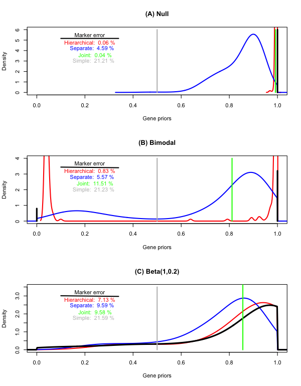
Figure 1: Comparison of four approaches to inferring prior probabilities, under three simulation scenarios (A,B, and C). Kernel density estimates of the resulting gene-specific probabilities are shown for continuous distributions; discrete distributions are shown by vertical lines. The distribution of the true gene-specific probabilities is colored black. The expected overall error in classifying null and alternative markers is also shown for each method and each simulation scenario.

To compare the Bayesian methods above with frequentist methods for multiple hypothesis testing, we compute a p-value for the null using Fisher’s exact test at each marker. We consider the following multiplicity adjustments for these p-values:

• Separate false-discovery rate (FDR) corrections for each gene, using the Benjamini-Hochberg method (Benjamini and Hochberg, 1995).

• An overall FDR correction for each marker.

• A two-step hierarchical hypothesis testing framework (Li and Ghosh, 2014) that uses the Hochberg (Hochberg, 1988) and Benjamini-Hochberg methods. This method controls the overall FDR while allowing for dependence within sets of hypotheses. In our context, a set corresponds to markers within a gene.

P-values and Bayesian posterior probabilities have fundamental differences in philosophy and interpretation, and are not directly comparable. Nonetheless, for illustration we compare the various approaches above by considering standard thresholds on the posterior probability, p-value or FDR that are used to classify markers as null or alternative. For Bayesian methods we use $0.5$ as a threshold on the posterior probability, and for the frequentist methods we use a significance threshold of $\alpha=0.05$. The resulting misclassification rates under each simulation scenario are shown in Table 1. Under the null model the hierarchical Bayesian approach gives very low error, similar to overall FDR corrections. Under the two scenarios with alternative markers the Bayesian hierarchical model performs substantially better than frequentist multiplicity corrections, which are overly conservative.

Table 1: Error in classifying null and alternative markers, using $0.5$ as a threshold for the posterior probability for Bayesian methods, and $0.05$ as an FDR or P-value threshold for frequentist methods using Fisher’s exact test. The average over $50$ replicate simulations is shown, and the resulting standard error is less than $0.05\%$ for all cells.

	Null	Bimodal	Beta $(1,0.2)$
Bayesian
Hierarchical	$0.01\%$	$0.07\%$	$3.92\%$
Separate	$0.50\%$	$1.68\%$	$4.87\%$
Joint	$0.01\%$	$6.89\%$	$5.34\%$
Simple	$5.07\%$	$8.72\%$	$7.82\%$
Frequentist
Two-step FDR	$0.01\%$	$7.73\%$	$6.30\%$
Separate FDR	$0.23\%$	$5.64\%$	$5.41\%$
Overall FDR	$0.01\%$	$7.15\%$	$5.78\%$
No correction	$2.91\%$	$7.50\%$	$6.49\%$

Figure 2 gives receiver operating characteristic (ROC) curves showing the proportion of markers with false positive or true positive classification (where ‘positive’ corresponds to the alternative) as the threshold on the posterior probability, p-value, or FDR is varied. Results are shown for the bimodal and Beta simulations; the ROC curve for the null simulation is trivial, as there are no true positives. In both cases the Bayesian hierarchical model has uniformly better classification performance than alternatives. The ROC curves for separate estimation are close, indicating that the rank ordering of probabilities are similar despite the improved accuracy of the hierarchical model.

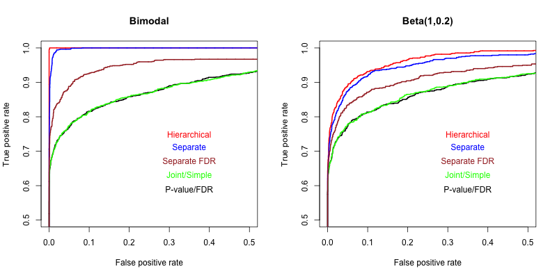
Figure 2: ROC curves obtained by varying the threshold on the posterior probability, p-value, or FDR for various methods. Curves are combined for the joint and simple Bayesian models, and for the uncorrected p-value and FDR, as the rank ordering of markers between these methods do not change.

A spreadsheet available online gives results for $99$ additional simulated datasets with varying sample size, number of genes, and distribution of gene-level probabilities. These results demonstrate the robustness of the hierarchical model.

5 Application to LGG-GBM Methylation

We implement our hierarchical gene-level prior model in a screen for differences in DNA methylation between lower grade gliomas (LGG) and glioblastoma multiforme (GBM) tumor samples that develop from astrocyte cells in the brain. Methylation is an epigenetic phenomenon that occurs at cytosine-phosphate-guanine (CpG) dinucleotide sites in the genome. Methylation is thought to play a significant role in LGG pathogenesis (TCGA Research Network, 2015) and GBM pathogenesis (TCGA Research Network, 2013), but the differences between the two tumor classes have not been well-characterized on a genome-wide scale. Both tumors are heterogenous and typically fatal, but a more complete understanding of their molecular differences is important, as LGGs often progress to GBMs and GBM patients have a much shorter survival time.

We use data from the Illumina HumanMethylation450 array, for 128 astrocyte derived LGG samples and 130 GBM samples, from The Cancer Genome Atlas. Measured CpG sites that have any missing data are removed, as are sites that map to intergenic regions. After filtering, $294,093$ CpG sites remain, that map to $24,358$ distinct genes. The number of sites in a gene ranges broadly from $1$ to $1017$. Array values at each site are between $0$ (no methylation) and $1$ (fully methylated across all cells in the tumor sample).

Several computational methods have been developed to screen for differential methylation levels between groups, based on array data (Jaffe et al., 2012; Maksimovic et al., 2015) or sequencing data (Sun et al., 2014; Feng et al., 2014; Wu et al., 2015). However, the focus on differential methylation levels between groups may miss other important differences between group distributions; for example, certain genomic regions have been shown to exhibit more variability in methylation, and hence greater epigenetic instability, among cancer cells than among normal cells (Hansen et al., 2011).

We test for differences in distribution between the LGG and GBM samples at each CpG site. Our testing model is described in detail in Lock and Dunson (2015), where it is implemented on comparatively sparse methylation data ($\approx 20,000$ sites) with a global prior and shown to compare favorably to frequentist and Bayesian alternatives. Briefly, the distribution at each site is modeled as a mixture of normal kernels, truncated between $0$ and $1$. The kernels are shared across CpG sites, and thus capture shared patterns of multi-modality and skewness that are typical in methylation array data. Under the null the kernel mixing weights at each site are assumed to be the same between the two groups, and under the alternative they are different. This provides a robust and consistent framework for testing differential distribution, and can identify important differences that are not captured by simply comparing mean methylation levels. Furthermore, the method facilitates interpretation by modeling the full distribution, with uncertainty, for each class. We incorporate hierarchical gene-level priors within the shared kernel testing model, and compute the full posterior via Gibbs sampling.

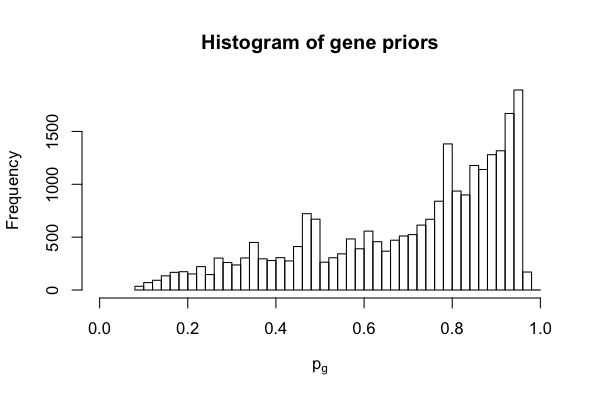
Figure 3: Histogram of estimated gene-specific probabilities $p_{g}$.

The estimated gene-level probabilities are shown in Figure 3. Their distribution resembles that in the simulation shown in Figure 1C. For the majority of genes the distribution between the two groups is inferred to be equal at most sites ($p_{g}\approx 1$). However, there is a substantial left tail, corresponding to genes in which a large number of sites are inferred to differ between the two groups. For illustration we focus on one such gene, BST2, which has $9$ measured CpG sites and an estimated gene-level probability of $p_{g}=0.198$. We select BST2 because it has been considered as a tangible target for immunotherapy in the treatment of GBM (Etcheverry et al., 2010), an independent comparison of GBM and normal samples found differences in BST2 methylation that correlate with gene expression (Wainwright et al., 2011), and BST2 methylation may play a role in the pathonogenesis of other cancers (Mahauad-Fernandez et al., 2014). Figure 4 shows the genomic location and posterior probability of group equality for the nine CpG sites in BST2, as well as group histograms and posterior densities for methylation at three sites.

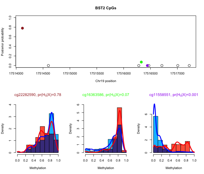
Figure 4: The top panel shows the estimated posterior probability of an association with GBM-LGG status for the 9 CpG sites measured in the gene BST2, with their corresponding genomic location. The lower panel shows the estimated densities for the GBM (blue) and LGG (red) groups for three sites; histograms of each group are shown, and their overlap is colored purple.

Given the large number of CpGs and corresponding genes with differential methylation distribution, we also investigate differences at a macro level. Figure 5 shows the site means and standard deviations within each group, for those sites with a posterior probability of equality less than $0.01$ (24.6% of all CpGs). Mean methylation levels at these sites are generally greater in the LGG samples than the GBM samples; this is concordant with findings in a smaller comparison of 1536 CpG sites in 807 genes (Laffaire et al., 2011). The distribution of standard deviations is more curious, as LGG samples show a larger number of sites with either very high variability or very low variability in comparison to the distribution for GBM.

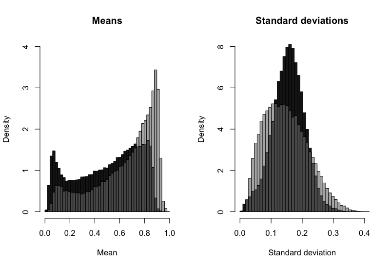
Figure 5: Histograms of summary statistics for every CpG site with a posterior probability of the null less than $0.01$, computed separately for the GBM (dark gray) and LGG (light gray) groups. Overlap between the two histograms is colored a neutral gray. The left panel show the site means, the right shows the site standard deviations.

Details regarding the association model and Gibbs sampling algorithm for posterior computation are given in Appendix A.

5.1 Validation

To asses the appropriateness of the hierarchical gene-level model, we consider the agreement of estimated gene-level probabilities and marker-level posteriors under cross validation. Specifically, we randomly select $10,000$ CpGs to leave out, and compute gene-level probabilities using the remaining $284,093$ CpGs. For each left out CpG, we measure the Kullback-Leibler divergence of its estimated gene-level probability under the reduced data from its CpG-level posterior probability under the full data. This can be interpreted as the gain of information or degree of “surprise” between a CpG’s posterior probability and its gene-level prior (Lindley, 1956). We repeat this process using a separately estimated prior probability for each gene, a single inferred prior probability, and a prior probability of $0.5$ (corresponding to the separate, joint and simple models in the Simulation Study). The hierarchical model yields the greatest agreement, with a mean Kullback-Leibler divergence of $0.451$; the separate model has a divergence of $0.482$, the joint model $0.560$, and the simple model $0.654$.

We also conduct two permutation studies, to further assess the appropriateness and flexibility of our gene-level model. First, we randomly permute the gene labels for each marker, so that there is no true gene-level dependence. The subsequent posterior means for the gene level prior probabilities $p_{g}$ are shown in the top-left panel of Figure 6. The estimates converge appropriately to a single global probability near $0.72$, in sharp contrast to the relatively dispersed estimates using the true data in Figure 2 of the main article. Second, we randomly permute the class labels but maintain the true gene labels, to generate a dataset with a global null but gene-level dependence. The subsequent posterior estimates are shown in the top-right panel of Figure 6, and cluster very close to $1$. In fact, all $294,093$ estimated site-specific posterior probabilities of the null are greater than $0.5$. Together, these results demonstrate that the hierarchical gene-level model appropriately shrinks gene-level priors toward a global pattern.

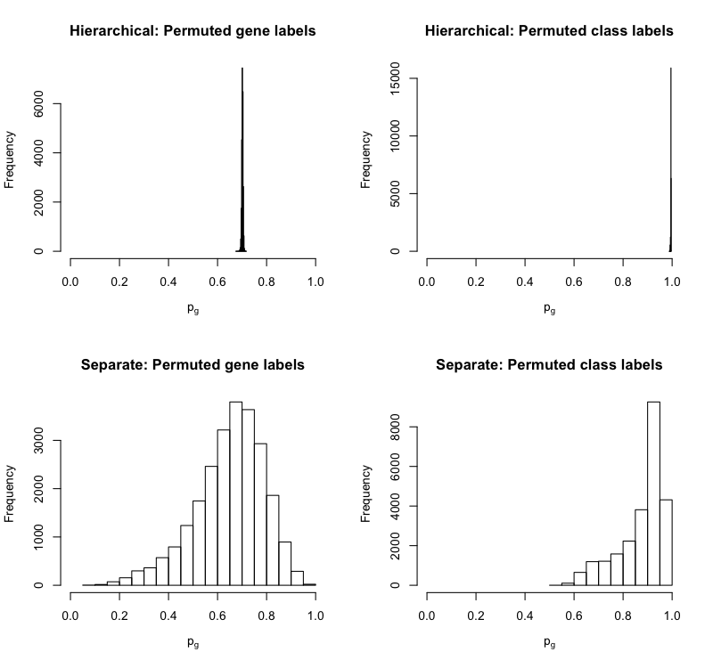
Figure 6: Histogram of hierarchically estimated and separately estimated gene-level priors after randomly permuting gene labels (left column), and after randomly permuting class labels (right column).

The estimated hierarchical gene-level probabilities closely approximate a single joint prior probability in Figure 6, where a joint prior is appropriate, but not for the true data. Thus, we conclude that a single joint model is an over-simplification for these data. We also compare the hierarchical gene-level prior probabilities under permutation with separate, independently estimated gene-level probabilities. The separately estimated probabilities are shown in the bottom row of 6. These have a lot of variability under both permutation scenarios, illustrating how independent consideration of the genes sacrifices accuracy by exaggerating gene effects.

6 Discussion

Borrowing information and incorporating prior knowledge in a principled and computationally feasible way is an important challenge for Bayesian genome- and epigenome-wide screening methods. Here we present a flexible and generally applicable hierarchical model for inferring gene-specific probabilities, which may be extended in several ways. Under our prior all markers within a gene have an equivalent probability of association. The incorporation of other marker-level information, such as gene promoter status for DNA methylation (Weber et al., 2005) or functional annotation (e.g., synonymous vs. non-synonymous) for genotype markers (Kichaev et al., 2014; Ruklisa et al., 2015), may improve posterior precision and interpretation. For example, a Dirichlet process model may be used for gene-level intercepts within a regression model for marker probabilities that includes additional prior covariates (Lewinger et al., 2007). Incorporating additional gene-level prior information, such as allowing greater dependence within known functional gene networks (Zhang et al., 2014), is also a promising direction of future work.

Our focus is on association testing. However, markers that are statistically associated with a given phenotype may not affect the phenotype directly, especially if markers are correlated (e.g., linkage disequilibrium in genetic data). Our gene-specific model and other prior information can also be used in the context of model inclusion probabilities, to select markers that have novel predictive power for a given phenotype and are therefore more likely to be causal (Wilson et al., 2010; Zhang et al., 2014; Duan and Thomas, 2013). However, computational scaling for high-throughput data is often a challenge in such problems; alternatively, markers identified via association testing may subsequently be included as phenotype predictors in a second stage model (Yazdani and Dunson, 2015).

In our context we consider multiple hypotheses, in which the hypotheses are naturally grouped by markers within a gene, but there are similar scenarios in other areas of genomics research. For example, when screening multiple genes for a phenotypic association (e.g., via microarray or RNA-seq data) the genes can be partitioned into groups based on pathways or other prior information. Frequentist methods that provide appropriate type I error control over genes and gene sets have been developed (Benjamini and Heller, 2008; Heller et al., 2009; Li and Ghosh, 2014), and these methods can be generalized to other problems that involve testing hypotheses over multiple sets. Broadly, our proposed model defines a general prior for multiple hypothesis testing within a Bayesian framework when the hypotheses can be partitioned into sets.

Appendix A Posterior Computation

This appendix provides details on posterior computation for the methylation screening application described in Section refapp.

First, we estimate and fix a dictionary of normal kernels truncated between $0$ and $1$, which will be used as mixture components for the density at each CpG site. These are estimated as described in Section 5 of Lock and Dunson (2015). In particular, the number of kernels is determined by out-of-sample cross validation of the log posterior density. For the present application this yields $K=8$ kernels that appropriately span the data range from $0$ to $1$.

Let $\Pi_{gm}^{(0)}=(\pi_{gm1}^{(0)},\ldots,\pi_{gmK}^{(0)})$ be the kernel probability weights that define the generative distribution for gene $g$ and site $m$ for group $0$, and let $\Pi_{gm}^{(1)}$ be the kernel probability weights for group $1$. Under the null model $H_{0gm}$, the mixing weights are the same for both groups: $\Pi_{gm}^{(0)}=\Pi_{gm}^{(1)}$. The kernel weights are assumed to be generated from a Dirichlet($\lambda$) distribution, where $\lambda$ is a hyper-parameter that is inferred during the kernel estimation stage and fixed. Under $H_{1gm}$, $\Pi_{gm}^{(0)}$ and $\Pi_{gm}^{(1)}$ are considered independent realizations from Dirichlet($\lambda$).

Under this framework, posterior draws from the gene-level prior model described in Section 3 of the main article are incorporated into Gibbs sampling for the kernel testing parameters. The full sampling algorithm is described below.

1. Draw the kernel that generated each observation $T^{(i)}_{gmn}\in{1,\ldots,K}$ for genes $g=1,\ldots,G$, markers $m=1,\ldots,M_{g}$, classes $i=0,1$ and samples $n=1,\ldots,N_{i}$. The conditional probability that the given value is realized from component $k$ is

   $$P(T_{mn}^{(i)}=k\mid X_{m}^{(i)},\Pi_{m}^{(i)})\propto\pi_{gmk}^{(i)}f(X_{gmn}^{(i)}|\mu_{k},\sigma_{k},[0,1]),$$

   where $f(\cdot)$ defines the density of a truncated normal distribution.

2. Designate null markers $H_{0,gm}$ for $g=1,\ldots,G$, $m=1,\ldots,M_{g}$. The conditional posterior probability is

   $$P(H_{0,gm}\mid X,Y,p_{g})=\frac{p_{g}\beta(\lambda)\beta(\vec{n}_{m}+\lambda)}{p_{g}\beta(\lambda)\beta(\vec{n}_{m}+\lambda)+(1-p_{g})\beta(\vec{n}_{m}^{(0)}+\lambda)\beta(\vec{n}_{m}^{(1)}+\lambda)},$$

   where $\vec{n}_{gm}^{(0)}=(n_{gm1}^{(0)},\ldots,n_{gmK}^{(0)})$ is the number of subjects in group $0$ that belong to each kernel $k$ in marker $g,m$, $\vec{n}_{gm}^{(1)}$ is defined similarly for group $1$, and $\vec{n}_{gm}=\vec{n}_{gm}^{(0)}+\vec{n}_{gm}^{(1)}$.

3. Draw weights $\{\Pi_{gm}^{(0)},\Pi_{gm}^{(1)}\}_{m=1}^{M}$. Under $H_{0,gm}$, $\Pi_{gm}^{(0)}=\Pi_{gm}^{(1)}\sim\text{Dirichlet}(\lambda+\vec{n}_{gm})$. Otherwise, $\Pi_{gm}^{(0)}\sim\text{Dirichlet}(\lambda+\vec{n}_{mg}^{(0)})$ and $\Pi_{gm}^{(1)}\sim\text{Dirichlet}(\lambda+\vec{n}_{mg}^{(1)})$.

4. Allocate gene-level Dirichlet indices $C_{g}$ for $g=1,\ldots,G$:

   $$P(C_{g}=h\mid\theta_{\cdot},H_{0,g\cdot})\propto\pi_{h}\theta_{h}^{S_{g}}(1-\theta_{h})^{M_{g}-S_{g}}$$

   where $S_{g}$ is the number of null markers in gene $g$, $S_{g}=\sum_{m=1}^{M_{g}}\mathbbm{1}(H_{0,gm})$.

5. Update the weights $\pi_{h}$ for $h=1,\ldots,H$. First, draw the stick-breaking weights $V_{1},\ldots,V_{H-1}$ by

   $$(V_{h}\mid C_{\cdot})\sim\mbox{Beta}\left(1+\sum_{g=1}^{G}\mathbbm{1}(C_{g}=h),\alpha+\sum_{g=1}^{G}\mathbbm{1}(C_{g}>h)\right),$$

   with $V_{H}=1$. Then set $\pi_{h}=V_{h}\prod_{l<h}(1-V_{l})$ for $h=1,\ldots,H$.

6. Update the atoms $\theta_{h}$ for $h=1,\ldots,H$:

   $$(\theta_{h}\mid C_{\cdot},H_{0,\cdot\cdot})\sim\mbox{Beta}\left(a+\tilde{S}_{h},b+\tilde{M}_{h}-\tilde{S}_{h}\right),$$

   where $\tilde{M}_{h}$ is the total number of markers in genes allocated to cluster $h$, and $\tilde{S}_{h}$ is the number of null markers:

   $$\tilde{M}_{h}=\sum_{\{g:C_{g}=h\}}M_{g}\,\,\,,\,\,\,\tilde{S}_{h}=\sum_{\{g:C_{g}=h\}}S_{g}.$$

   Set $p_{g}=\theta_{C_{g}}$ for $g=1,\ldots,G$.

We use a simple uniform prior for the base distribution of $p_{g}$ ($a=b=1$).

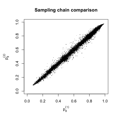
Figure 7: Scatterplot of estimated gene-level prior from two independent sampling chains.

For the high-throughput data considered, computing is not trivial, costing approximately 30 seconds per Gibbs cycle. However, less than 1% of computing time is spent on the draws for the gene-level prior parameters (steps 4-6). We find that draws mix well and converge very quickly to a stationary posterior. We run two parallel chains, with different initializations, for 1000 cycles, with the first 200 treated as burn-in. Figure 7 shows good agreement of estimated gene-level prior probabilities between the two chains.

References

- Balding [2006] D. J. Balding. A tutorial on statistical methods for population association studies. Nature Reviews Genetics, 7(10):781–791, 2006.
- Benjamini and Heller [2008] Y. Benjamini and R. Heller. Screening for partial conjunction hypotheses. Biometrics, 64(4):1215–1222, 2008.
- Benjamini and Hochberg [1995] Y. Benjamini and Y. Hochberg. Controlling the false discovery rate: a practical and powerful approach to multiple testing. Journal of the Royal Statistical Society: Series B, 57(1):289–300, 1995.
- Duan and Thomas [2013] L. Duan and D. C. Thomas. A bayesian hierarchical model for relating multiple snps within multiple genes to disease risk. International Journal of Genomics, 2013:406217, 2013.
- Etcheverry et al. [2010] A. Etcheverry, M. Aubry, M. De Tayrac, E. Vauleon, R. Boniface, F. Guenot, S. Saikali, A. Hamlat, L. Riffaud, P. Menei, et al. DNA methylation in glioblastoma: impact on gene expression and clinical outcome. BMC Genomics, 11(1):701, 2010.
- Feng et al. [2014] H. Feng, K. N. Conneely, and H. Wu. A bayesian hierarchical model to detect differentially methylated loci from single nucleotide resolution sequencing data. Nucleic Acids Research, 42(8):e69, 2014.
- Ferguson [1973] T. S. Ferguson. A Bayesian analysis of some nonparametric problems. The Annals of Statistics, 1(2):209–230, 1973.
- Hansen et al. [2011] K. D. Hansen, W. Timp, H. C. Bravo, S. Sabunciyan, B. Langmead, O. G. McDonald, B. Wen, H. Wu, Y. Liu, D. Diep, et al. Increased methylation variation in epigenetic domains across cancer types. Nature Genetics, 43(8):768–775, 2011.
- Heller et al. [2009] R. Heller, E. Manduchi, G. R. Grant, and W. J. Ewens. A flexible two-stage procedure for identifying gene sets that are differentially expressed. Bioinformatics, 25(8):1019–1025, 2009.
- Hochberg [1988] Y. Hochberg. A sharper Bonferroni procedure for multiple tests of significance. Biometrika, 75(4):800–802, 1988.
- Ishwaran and James [2001] H. Ishwaran and L. F. James. Gibbs sampling methods for stick-breaking priors. Journal of the American Statistical Association, 96(453):161––173, 2001.
- Jaffe et al. [2012] A. E. Jaffe, P. Murakami, H. Lee, J. T. Leek, M. D. Fallin, A. P. Feinberg, and R. A. Irizarry. Bump hunting to identify differentially methylated regions in epigenetic epidemiology studies. International Journal of Epidemiology, 41(1):200–209, 2012.
- Kichaev et al. [2014] G. Kichaev, W. Yang, S. Lindstrom, F. Hormozdiari, E. Eskin, A. Price, P. Kraft, and B. Pasaniuc. Integrating functional data to prioritize causal variants in statistical fine-mapping studies. PLoS Genetics, 10(10):e1004722, 2014.
- Laffaire et al. [2011] J. Laffaire, S. Everhard, A. Idbaih, E. Criniere, Y. Marie, A. de Reynies, R. Schiappa, K. Mokhtari, K. Hoang-Xuan, M. Sanson, et al. Methylation profiling identifies 2 groups of gliomas according to their tumorigenesis. Neuro-Oncology, 13(1):84–98, 2011.
- Lewinger et al. [2007] J. P. Lewinger, D. V. Conti, J. W. Baurley, T. J. Triche, and D. C. Thomas. Hierarchical bayes prioritization of marker associations from a genome-wide association scan for further investigation. Genetic Epidemiology, 31(8):871–882, 2007.
- Li and Ghosh [2014] Y. Li and D. Ghosh. A two-step hierarchical hypothesis set testing framework, with applications to gene expression data on ordered categories. BMC Bioinformatics, 15(1):108, 2014.
- Lindley [1956] D. V. Lindley. On a measure of the information provided by an experiment. The Annals of Mathematical Statistics, pages 986–1005, 1956.
- Liu et al. [2010] J. Z. Liu, A. F. Mcrae, D. R. Nyholt, S. E. Medland, N. R. Wray, K. M. Brown, N. K. Hayward, G. W. Montgomery, P. M. Visscher, N. G. Martin, et al. A versatile gene-based test for genome-wide association studies. The American Journal of Human Genetics, 87(1):139–145, 2010.
- Lock and Dunson [2015] E. F. Lock and D. B. Dunson. Shared kernel Bayesian screening. Biometrika, 102(4):829–842, 2015.
- Mahauad-Fernandez et al. [2014] W. D. Mahauad-Fernandez, N. C. Borcherding, W. Zhang, and C. M. Okeoma. Bone marrow stromal antigen 2 (BST-2) DNA is demethylated in breast tumors and breast cancer cells. PloS One, 10(4):e0123931, 2014.
- Maksimovic et al. [2015] J. Maksimovic, J. A. Gagnon-Bartsch, T. P. Speed, and A. Oshlack. Removing unwanted variation in a differential methylation analysis of Illumina HumanMethylation450 array data. Nucleic Acids Research, page gkv526, 2015.
- Pan et al. [2014] W. Pan, J. Kim, Y. Zhang, X. Shen, and P. Wei. A powerful and adaptive association test for rare variants. Genetics, 197(4):1081–1095, 2014.
- Park et al. [2010] J.-H. Park, S. Wacholder, M. H. Gail, U. Peters, K. B. Jacobs, S. J. Chanock, and N. Chatterjee. Estimation of effect size distribution from genome-wide association studies and implications for future discoveries. Nature Genetics, 42(7):570–575, 2010.
- Rowntree and Harris [2003] R. K. Rowntree and A. Harris. The phenotypic consequences of cftr mutations. Annals of Human Genetics, 67(5):471–485, 2003.
- Ruklisa et al. [2015] D. Ruklisa, J. S. Ware, R. Walsh, D. J. Balding, and S. A. Cook. Bayesian models for syndrome-and gene-specific probabilities of novel variant pathogenicity. Genome Medicine, 7:120, 2015.
- Scott et al. [2010] J. G. Scott, J. O. Berger, et al. Bayes and empirical-Bayes multiplicity adjustment in the variable-selection problem. The Annals of Statistics, 38(5):2587–2619, 2010.
- Sethuraman [1994] J. Sethuraman. A constructive definition of Dirichlet priors. Statistica Sinica, 4:639–650, 1994.
- Stephens and Balding [2009] M. Stephens and D. J. Balding. Bayesian statistical methods for genetic association studies. Nature Reviews Genetics, 10(10):681–690, 2009.
- Sun et al. [2014] D. Sun, Y. Xi, B. Rodriguez, H. J. Park, P. Tong, M. Meong, M. A. Goodell, and W. Li. MOABS: model based analysis of bisulfite sequencing data. Genome Biology, 15(2):38, 2014.
- TCGA Research Network [2013] TCGA Research Network. The somatic genomic landscape of glioblastoma. Cell, 155(2):462–477, 2013.
- TCGA Research Network [2015] TCGA Research Network. Comprehensive, integrative genomic analysis of diffuse lower-grade gliomas. New England Journal of Medicine, 372:2481–2498, 2015.
- Verzilli et al. [2008] C. Verzilli, T. Shah, J. P. Casas, J. Chapman, M. Sandhu, S. L. Debenham, M. S. Boekholdt, K. T. Khaw, N. J. Wareham, R. Judson, et al. Bayesian meta-analysis of genetic association studies with different sets of markers. The American Journal of Human Genetics, 82(4):859–872, 2008.
- Visscher et al. [2012] P. M. Visscher, M. A. Brown, M. I. McCarthy, and J. Yang. Five years of GWAS discovery. The American Journal of Human Genetics, 90(1):7–24, 2012.
- Wainwright et al. [2011] D. A. Wainwright, I. V. Balyasnikova, Y. Han, and M. S. Lesniak. The expression of BST2 in human and experimental mouse brain tumors. Experimental and Molecular Pathology, 91(1):440–446, 2011.
- Wakefield [2009] J. Wakefield. Bayes factors for genome-wide association studies: comparison with p-values. Genetic Epidemiology, 33(1):79–86, 2009.
- Wang et al. [2012] D. Wang, L. Yan, Q. Hu, L. E. Sucheston, M. J. Higgins, C. B. Ambrosone, C. S. Johnson, D. J. Smiraglia, and S. Liu. IMA: an R package for high-throughput analysis of illumina’s 450k infinium methylation data. Bioinformatics, 28(5):729–730, 2012.
- Weber et al. [2005] M. Weber, J. J. Davies, D. Wittig, E. J. Oakeley, M. Haase, W. L. Lam, and D. Schuebeler. Chromosome-wide and promoter-specific analyses identify sites of differential DNA methylation in normal and transformed human cells. Nature Genetics, 37(8):853–862, 2005.
- Welter et al. [2014] D. Welter, J. MacArthur, J. Morales, T. Burdett, P. Hall, H. Junkins, A. Klemm, P. Flicek, T. Manolio, L. Hindorff, et al. The nhgri GWAS catalog, a curated resource of SNP-trait associations. Nucleic Acids Research, 42(D1):D1001–D1006, 2014.
- Wen et al. [2014] X. Wen, M. Stephens, et al. Bayesian methods for genetic association analysis with heterogeneous subgroups: From meta-analyses to gene–environment interactions. The Annals of Applied Statistics, 8(1):176–203, 2014.
- Wilson et al. [2010] M. A. Wilson, E. S. Iversen, M. A. Clyde, S. C. Schmidler, and J. M. Schildkraut. Bayesian model search and multilevel inference for SNP association studies. The Annals of Applied Statistics, 4(3):1342–1364, 2010.
- Wojcik et al. [2015] G. L. Wojcik, W. L. Kao, and P. Duggal. Relative performance of gene-and pathway-level methods as secondary analyses for genome-wide association studies. BMC Genetics, 16(1):34, 2015.
- Wu et al. [2015] H. Wu, T. Xu, H. Feng, L. Chen, B. Li, B. Yao, Z. Qin, P. Jin, and K. N. Conneely. Detection of differentially methylated regions from whole-genome bisulfite sequencing data without replicates. Nucleic Acids Research, 43(21):e141, 2015.
- Wu et al. [2011] M. C. Wu, S. Lee, T. Cai, Y. Li, M. Boehnke, and X. Lin. Rare-variant association testing for sequencing data with the sequence kernel association test. The American Journal of Human Genetics, 89(1):82–93, 2011.
- Xu et al. [2012] J. Xu, A. Yuan, and G. Zheng. Bayes factor based on the trend test incorporating hardy–weinberg disequilibrium: more power to detect genetic association. Annals of Human Genetics, 76(4):301–311, 2012.
- Yazdani and Dunson [2015] A. Yazdani and D. B. Dunson. A hybrid Bayesian approach for genome-wide association studies on related individuals. Bioinformatics, 31(24):3890–3896, 2015.
- Zhang et al. [2014] X. Zhang, F. Xue, H. Liu, D. Zhu, B. Peng, J. L. Wiemels, and X. Yang. Integrative Bayesian variable selection with gene-based informative priors for genome-wide association studies. BMC Genetics, 15(1):130, 2014.