How to resum perturbative series in 3d $\mathcal{N}=2$ Chern-Simons matter theories

Abstract

Continuing the work arXiv:1603.06207, we study perturbative series in general 3d $\mathcal{N}=2$ supersymmetric Chern-Simons matter theory with $U(1)_{R}$ symmetry, which is given by a power series expansion of inverse Chern-Simons levels. We find that the perturbative series are usually non-Borel summable along positive real axis for various observables. Alternatively we prove that the perturbative series are always Borel summable along negative (positive) imaginary axis for positive (negative) Chern-Simons levels. It turns out that the Borel resummations along this direction are the same as exact results and therefore correct ways of resumming the perturbative series.

I Introduction

Chern-Simons (CS) theories coupled to matters play important roles in high energy physics and condensed matter physics. When CS levels are finite, the theories are strongly coupled and systematic analysis is restricted. While one can always setup perturbation theories in the CS theories by expanding observables around infinite CS levels, the perturbative series are usually divergent as in typical interacting quantum field theory (QFT) Dyson:1952tj . Therefore it is generically hard to obtain information on the strongly coupled systems from the perturbative series. In this paper we address this problem and discuss that we can obtain exact results by appropriately resumming the perturbative series in 3d $\mathcal{N}=2$ supersymmetric (SUSY) CS matter theories.

One of standard methods to resum divergent series is Borel resummation. Given a perturbative series $\sum_{\ell=0}^{\infty}c_{\ell}g^{a+\ell}$ of a quantity $I(g)$, its Borel resummation along the direction $\theta$ is defined by

$$\mathcal{S}_{\theta}I(g)=\int_{0}^{\infty e^{i\theta}}dt\ e^{-\frac{t}{g}}\mathcal{B}I(t).$$ (1)

Here $\mathcal{B}I(t)$ is analytic continuation of the formal Borel transformation $\sum_{\ell=0}^{\infty}\frac{c_{\ell}}{\Gamma(a+\ell)}t^{a+\ell-1}$ after performing the summation. While perturbative series in typical interacting QFT is expected to be non-Borel summable along positive real axis due to singularities in $\mathcal{B}I(t)$ 'tHooft:1977am , it is natural to ask when perturbative series is Borel summable along $\mathbb{R}_{+}$ and if it is non-Borel summable, what is a correct way to resum the perturbative series. This is not just a technical question but physically fundamental question since this is related to how to define interacting QFT’s.

In Honda:2016mvg the author initiated to address this question. We have proven that perturbative series in 4d $\mathcal{N}=2$ and 5d $\mathcal{N}=1$ SUSY gauge theories with Lagrangians are Borel summable along positive real axis for various observables . This result for the 4d $\mathcal{N}=2$ theories is expected from a recent proposal on a semi-classical realization of infrared renormalons Argyres:2012vv , where the semiclassical solution does not exist in the $\mathcal{N}=2$ theories (see also Dunne:2012ae ). Then it is natural to apply the technique in Honda:2016mvg to another class of theories. In this paper we study perturbative series in general 3d $\mathcal{N}=2$ SUSY CS matter theories with $U(1)_{R}$ symmetry in terms of inverse CS levels (see Russo:2012kj for studies of 3d $\mathcal{N}=6$ case). We apply the technique in Honda:2016mvg to localization formula Pestun:2007rz for various observables in 3d $\mathcal{N}=2$ CS matter theories.

Nevertheless we find highly different results from the 4d $\mathcal{N}=2$ and 5d $\mathcal{N}=1$ theories. First of all we find that perturbative series are usually not Borel summable along $\mathbb{R}_{+}$ for various observables. Alternatively we prove that the perturbative series are always Borel summable along negative imaginary axis for positive CS levels and positive imaginary axis for negative CS levels. We also prove that the Borel resummations along this direction are the same as exact results . Our main result is schematically written as (more precise statement is (20))

$$\mathcal{O}(g)=\mathcal{S}_{\frac{-\pi{\rm sgn}(k)}{2}}\mathcal{O}(g)=\int_{0}^{-i{\rm sgn}(k)\infty}dt\ e^{-\frac{t}{g}}\mathcal{B}\mathcal{O}(t),$$ (2)

where $g\propto 1/|k|$ with CS level $k$ and $\mathcal{B}\mathcal{O}(t)$ is Borel transformation of small-$g$ expansion of the observable $\mathcal{O}(g)$. This means that exact results are given by the Borel resummations along the direction $\theta=-\pi{\rm sgn}(k)/2$. In sec. II we proove the results (2) for $S^{3}$ partition function, SUSY Wilson loops, Bremsstrahrung function, two-point function of $U(1)$ flavor symmetry currents, partition function on on squashed lens space and two-point function of stress tensor.

Our rerult (2) is quite surprising in the following reason. When the perturbative series are not Borel summable along $\mathbb{R}_{+}$, we usually consider a possibility of cancellations of the perturbative ambiguities by contributions from other saddle points such as instantons or perform more complicated analysis such as median resummation to find a correct integral contour. We find that we can skip the complicated analyzes and directly find the correct integral contour though understanding from the usual analyzes should be important. We expect that our result is very important also for understanding non-SUSY CS matter theories. While we do not know if the perturbative series in the non-SUSY theories are Borel summable along the contour in (2), it is natural to expect that this choice of the contour makes analysis highly simplified .

II Derivation of results

II.1 Partition function on $S^{3}$

Suppose 3d $\mathcal{N}=2$ CS matter theory with a semi-simple gauge group $G=G_{1}\times\cdots\times G_{n}$, which is coupled to chiral multiplets of representations $(\mathbf{R_{1}},\cdots,\mathbf{R_{N_{f}}})$ with $R$-charges $(\Delta_{1},\cdots,\Delta_{N_{f}})$. Applying the localization method Pestun:2007rz , the $S^{3}$ partition function of this theory is given by Kapustin:2009kz

$$Z_{S^{3}}(g)=\int_{-\infty}^{\infty}d^{|G|}\sigma\ Z_{\rm cl}(\sigma)Z_{\rm 1loop}(\sigma),$$ (3)

where

$$Z_{\rm cl}(\sigma)=\exp{\Bigl{[}\sum_{p=1}^{n}\frac{i{\rm sgn}(k_{p})}{g_{p}}{\rm tr}(\sigma^{(p)})^{2}\Bigr{]}},$$

$$Z_{\rm 1loop}(\sigma)=\frac{\prod_{\alpha\in{\rm root}_{+}}4\sinh^{2}{(\pi\alpha\cdot\sigma)}}{\prod_{m=1}^{N_{f}}\prod_{\rho_{m}\in\mathbf{R_{m}}}s_{1}\left(\rho_{m}\cdot\sigma-i(1-\Delta_{m})\right)},$$

$$s_{b}(z)=\prod_{m=0}^{\infty}\prod_{n=0}^{\infty}\frac{mb+nb^{-1}+Q/2-iz}{mb+nb^{-1}+Q/2+iz}.$$ (4)

The parameter $g_{p}$ is proportional to $1/|k|$. Now we are interested in small-$g_{p}$ expansion of $Z_{S^{3}}(g)$:

$$Z_{S^{3}}(g)=\sum_{\{\ell_{p}\}=0}^{\infty}c_{\ell_{1},\cdots,\ell_{n}}\prod_{p=1}^{n}g_{p}^{\frac{{\rm dim}(G_{p})}{2}+\ell_{p}}.$$ (5)

We will see that the perturbative series are usually non-Borel summable along $\mathbb{R}_{+}$ but always Borel summable along negative (positive) imaginary axis for $k_{p}>0$ ($k_{p}<0$).

$U(N)_{k}$ adjoint SQCD

For simplicity of explanations, we begin with the 3d $\mathcal{N}=2$ $U(N)_{k}$ SQCD with $N_{f}$ fundamental (R-charge $\Delta_{f}$), $\bar{N}_{f}$ anti-fundamental (R-charge $\bar{\Delta}_{f}$) and $N_{a}$ adjoint chiral multiplets (R-charge $\Delta_{a}$). We will discuss general case later. The $S^{3}$ partition function of this theory is

$$Z_{\rm SQCD} = \int_{-\infty}^{\infty}d^{N}\sigma\ \prod_{j=1}^{N}e^{\frac{i{\rm sgn}(k)}{g}\sigma_{j}^{2}}\frac{s_{1}^{\bar{N}_{f}}\left(\sigma_{j}+i(1-\bar{\Delta}_{f})\right)}{s_{1}^{N_{f}}\left(\sigma_{j}-i(1-\Delta_{f})\right)}$$ (6)

$$\times\frac{\prod_{i<j}4\sinh^{2}{(\pi(\sigma_{i}-\sigma_{j}))}}{\prod_{i,j}s_{1}^{N_{a}}\left(\sigma_{i}-\sigma_{j}-i(1-\Delta_{a})\right)}.$$

Now we apply the technique in Honda:2016mvg to this and investigate properties of the small-$g$ expansion of $Z_{\rm SQCD}$. To do this, let us make the following change of variables

$$\sigma_{i}=\sqrt{\tau}\hat{x}_{i},$$ (7)

where $\hat{\mathbf{x}}=(\hat{x}_{1},\cdots,\hat{x}_{N})$ is the unit vector spanning unit $S^{N-1}$. Then we rewrite the partition function as

$$Z_{\rm SQCD} = \int_{0}^{\infty}d\tau\ e^{\frac{i{\rm sgn}(k)}{g}\tau}f(\tau)$$ (8)

$$= i{\rm sgn}(k)\int_{0}^{-i{\rm sgn}(k)\infty}dt\ e^{-\frac{t}{g}}f(i{\rm sgn}(k)t),$$

where

$$f(\tau)=\frac{\tau^{\frac{N^{2}}{2}-1}}{2}\int_{S^{N-1}}d^{N-1}\hat{x}\ h(\tau,\hat{x}),$$

$$h(\tau,\hat{x})=\frac{Z_{\rm VdM}(\hat{x})Z_{\rm 1loop}(\sqrt{\tau}\hat{x})}{Z_{\rm VdM}(\sqrt{\tau}\hat{x})},$$

$$Z_{\rm VdM}(\sigma)=\prod_{\alpha\in{\rm root}_{+}}(\pi\alpha\cdot\sigma)^{2}.$$ (9)

Note that (8) is similar to the Borel resummation formula (1) with the direction $\theta=-\pi{\rm sgn}(k)/2$. Therefore one might wonder whether $f(\tau)$ is related to the Borel transformation of the original perturbative series. This question is technically equivalent to whether $f(\tau)$ consists purely of convergent power series of $\tau$ and it is very nontrivial in general.

Nevertheless we can indeed prove in a similar way to Honda:2016mvg that $f(\tau)$ has the following relation to the Borel transformation

$$i{\rm sgn}(k)f(\tau)=\mathcal{B}Z_{\rm SQCD}(-i{\rm sgn}(k)\tau),$$ (10)

where $\mathcal{B}Z_{\rm SQCD}(t)$ is the Borel transformation of the small-$g$ expansion of $Z_{\rm SQCD}$. Here we just write down an outline of the proof (see appendix for details): (I) We show uniform convergence of the small-$\tau$ expansion of $h(\tau,\hat{x})$. (II) The uniform convergence tells us that $h(\tau,\hat{x})$ is the same as analytic continuation of the convergent series and we can exchange the order of the power series expansion of $h(\tau,\hat{x})$ and the integration over $\hat{x}$. (III) The integral transformation (8) guarantees that the coefficient of the perturbative series of $f(\tau)$ at $\mathcal{O}(\tau^{\frac{N^{2}}{2}+\ell-1})$ is given by $(-i{\rm sgn}(k))^{\ell}c_{\ell}/\Gamma(\frac{N^{2}+\ell}{2})$ . Thus we conclude

$$Z_{\rm SQCD}=\int_{0}^{-i{\rm sgn}(k)\infty}dt\ e^{-\frac{t}{g}}\mathcal{B}Z_{\rm SQCD}(t).$$ (11)

Since the Borel transformation does not have singularities along the integral contour , the small-$g$ expansion of $Z_{\rm SQCD}$ is Borel summable along the direction $\theta=-{\rm sgn}(k)\pi/2$. Eq. (11) also tells us that the Borel resummation with this direction gives the exact result.

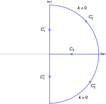
Figure 1: The integral contour, which relates the Borel resummation along the imaginary axis to the one along the real positive axis.

When does the pertubative series become Borel summable along $\mathbb{R}_{+}$? Since $t\in\mathbb{R}_{+}$ corresponds to $\sigma_{j}\in(-e^{\frac{\pi i}{4}{\rm sgn}(k)}\infty,e^{\frac{\pi i}{4}{\rm sgn}(k)}\infty)$ in (6), a sufficient condition for this is absence of singularities in the one-loop determinant along this line, namely $N_{a}=0$ (or $\Delta_{a}=1$). Next we ask when the perturbative series is Borel summable along $\mathbb{R}_{+}$, how this is related to the exact result. To answer this question, we need to change the integral contour to $\mathbb{R}_{+}$ as in fig. 1. There is a subtlety on this, which is related to CS level shift coming from integration over massive fermions (see e.g. Kao:1995gf ). When the integral variables $\sigma$ are very large, the contribution from chiral multiplet becomes

$$\frac{1}{s_{1}(\sigma-i(1-\Delta))}=\exp{\Biggl{[}\frac{i\pi{\rm sgn}(\sigma)}{2}\sigma^{2}+\mathcal{O}(|\sigma|)\Biggr{]}}.$$ (12)

This effectively shifts the CS level by ${\rm sgn}(\sigma)/2$ and the shift in the adjoint SQCD is totally ${\rm sgn}(\sigma_{j})(N_{f}-\bar{N}_{f})/2$. Hence the contribution from $C_{2}^{\pm}$ disappears for $|k|>|N_{f}-\bar{N}_{f}|/2$. If we consider this region, then we find

$$Z_{\rm SQCD}=\left(\int_{0}^{\infty}dt+\oint_{C}dt\right)e^{-\frac{t}{g}}\mathcal{B}Z_{\rm SQCD}(t),$$ (13)

where the integral contour $C$ is $C=C_{1}^{+}+C_{2}^{+}+C_{3}$ for $k>0$ and $C=C_{1}^{-}+C_{2}^{-}+C_{3}$ for $k<0$. Thus the Borel resummation along $\mathbb{R}_{+}$ gives the exact result when the second term is zero. A sufficient condition for this is again $N_{a}=0$.

It is worth looking at $N_{f}=\bar{N}_{f}=N_{a}=0$ case, which corresponds to the $\mathcal{N}=2$ CS theory without chiral multiplets and the same as the pure CS theory up to level shift. Since $Z_{\rm 1loop}$ does not have poles for this case, the Borel transformation also does not have any poles. This reflects the fact that the perturbative series in the pure CS theory is convergent.

General 3d $\mathcal{N}=2$ CS matter theory

Extension to general 3d $\mathcal{N}=2$ CS matter theory is straightforward. First we insert delta function constraint $\Delta(\sigma)$ to the integrand such that the following coordinate spans sphere with radius $\sqrt{\tau_{p}}$

$$\sigma_{i}^{(p)}=\sqrt{\tau_{p}}\hat{x}_{i}^{(p)}.$$ (14)

Then the partition function again takes the form of (8) extended to multi-variables:

$$Z_{S^{3}} = \int_{0}^{\infty}d^{n}\tau\ e^{\sum_{p=1}^{n}\frac{i{\rm sgn}(k_{p})}{g_{p}}\tau_{p}}f(\tau)$$

$$= \Biggl{[}\prod_{p=1}^{n}i{\rm sgn}(k_{p})\int_{0}^{-i{\rm sgn}(k_{p})\infty}dt_{p}e^{-\frac{t_{p}}{g_{p}}}\Biggr{]}f(i{\rm sgn}(k)t),$$

where

$$f(\tau)=\frac{\tau^{\frac{{\rm dim}(G)}{2}-1}}{2^{n}}\int_{\rm sphere}d\hat{x}\ \Delta(\hat{x})h(\tau,\hat{x}),$$

$$h(\tau,\hat{x})=\left.\frac{Z_{\rm VdM}(\hat{x})Z_{\rm 1loop}(\sigma)}{Z_{\rm VdM}(\sigma)}\right|_{\sigma_{i}^{(p)}=\sqrt{\tau_{p}}\hat{x}_{i}^{(p)}},$$

$$\tau^{\frac{{\rm dim}(G)}{2}-1}=\prod_{p=1}^{n}\tau_{p}^{\frac{{\rm dim}(G_{p})}{2}-1}.$$ (16)

We can always prove that $f(\tau)$ is related to the Borel transformation of the original perturbative series as

$$\Biggl{[}\prod_{p=1}^{n}i{\rm sgn}(k_{p})\Biggr{]}f(\{\tau_{p}\})=\mathcal{B}Z_{S^{3}}\left(\{-i{\rm sgn}(k_{p})\tau_{p}\}\right),$$ (17)

since small-$\tau_{p}$ expansion of $h(\tau,\hat{x})$ is uniform convergent if $Z_{S^{3}}$ is well-defined. This immediately leads us to

$$Z_{S^{3}}(g)=\Biggl{[}\prod_{p=1}^{n}\int_{0}^{-i{\rm sgn}(k_{p})\infty}dt_{p}e^{-\frac{t_{p}}{g_{p}}}\Biggr{]}\mathcal{B}Z_{S^{3}}(t),$$ (18)

which is generalization of (11).

A sufficient condition for Borel summability along $\mathbb{R}_{+}$ is again absence of singularities along $\sigma_{j}\in(-e^{\frac{\pi i}{4}{\rm sgn}(k)}\infty,e^{\frac{\pi i}{4}{\rm sgn}(k)}\infty)$ in $Z_{\rm 1loop}$. When the perturbative series is Borel summable along $\mathbb{R}_{+}$ and “level shift” is not so very large, we obtain

$$Z_{S^{3}}(g)=\Biggl{[}\prod_{p=1}^{n}\Bigl{(}\int_{0}^{\infty}dt_{p}+\oint_{C}dt_{p}\Bigr{)}e^{-\frac{t_{p}}{g_{p}}}\Biggr{]}\mathcal{B}Z_{S^{3}}(t).$$ (19)

If the second term is zero, the Borel resummation along $\mathbb{R}_{+}$ is the same as the exact result. In the rest of this paper, we prove our main result for various observables:

$$\mathcal{O}(g)=\Biggl{[}\prod_{p=1}^{n}\int_{0}^{-i{\rm sgn}(k_{p})\infty}dt_{p}e^{-\frac{t_{p}}{g_{p}}}\Biggr{]}\mathcal{B}\mathcal{O}(t).$$ (20)

II.2 Other observables

Supersymmetric Wilson loop

We can generalize the above considerations to other observables. Let us begin with the Wilson loop

$$W_{\mathbf{R}}(C)={\rm tr}_{\mathbf{R}}P\exp{\Biggl{[}\oint_{C}ds(iA_{\mu}\dot{x}^{\mu}+\sigma|\dot{x}|)\Biggr{]}},$$ (21)

with the adjoint scalar $\sigma$ in vector multiplet The Wilson loop preserves two supercharges when the contour $C$ is the great circle of $S^{3}$. Applying the localization method, VEV of the Wilson loop is given by

$$\langle W_{\mathbf{R}}({\rm Circle})\rangle=\langle{\rm tr}_{\mathbf{R}}e^{\sigma}\rangle_{\rm M.M.},$$ (22)

where $\langle\cdots\rangle_{\rm M.M.}$ denotes VEV in the matrix model (3). This is just linear combination of exponential function of $\sigma$ and we can obviously write the Wilson loop as in (20).

Bremsstrahrung function in SCFT on $\mathbb{R}^{3}$

Bremsstrahrung function $B$ determines an energy radiated by accelerating quarks in small velocities as $E=2\pi B\int dt\dot{v}^{2}$. It was conjectured that $B$ in 3d $\mathcal{N}=2$ superconformal theory is given by Lewkowycz:2013laa

$$B(g)=\frac{1}{4\pi^{2}}\left.\frac{\partial}{\partial b}\log\langle{\rm tr}e^{ba}\rangle_{\rm M.M.}\right|_{b=1},$$ (23)

which is technically derivative of the Wilson loop in fundamental representation with winding number $b$. As in the Wilson loop, we can also rewrite $B(g)$ as in (20).

Two-point function of $U(1)$ flavor symmetry currents in SCFT on $\mathbb{R}^{3}$

Next we consider two-point function of the $U(1)$ flavor symmetry current $j_{\mu}^{a}$ for superconformal case. The 3d conformal symmetry fixes the two-point function as

$$\langle j_{a}^{\mu}(x)j_{b}^{\nu}(0)\rangle=\frac{\tau_{ab}}{16\pi^{2}}(\delta^{\mu\nu}\partial^{2}-\partial^{\mu}\partial^{\nu})\frac{1}{x^{2}}+\frac{i\kappa_{ab}}{2\pi}\epsilon^{\mu\nu\rho}\partial_{\rho}\delta^{(3)}(x),$$ (24)

where $\tau_{ab}(g)$ and $\kappa_{ab}(g)$ are independent of $x$ but nontrivially dependent on parameters. We can exactly compute $\tau_{ab}(g)$ and $\kappa_{ab}(g)$ by the localization Closset:2012vg . This is generated by the $S^{3}$ partition function $Z_{S^{3}}(m,g)$ deformed by real mass $\{m_{a}\}$ associated with the $U(1)$ symmetries:

$$\tau_{ab}(g)=-\frac{2}{\pi^{2}}{\rm Re}\left[\frac{1}{Z_{S^{3}}(0,g)}\frac{\partial^{2}Z_{S^{3}}(m,g)}{\partial m_{a}\partial m_{b}}\right]_{\{m_{a}\}=0},$$

$$\kappa_{ab}(g)=\frac{1}{2\pi}{\rm Im}\left[\frac{1}{Z_{S^{3}}(0,g)}\frac{\partial^{2}Z_{S^{3}}(m,g)}{\partial m_{a}\partial m_{b}}\right]_{\{m_{a}\}=0}.$$ (25)

Repeating the argument on $Z_{S^{3}}$, we can show that $\tau_{ab}(g)$ and $\kappa_{ab}(g)$ satisfy (20).

Partition function and Wilson loop on Squashed $S^{3}$

Let us consider partition function on squashed sphere $S^{3}_{b}$ with the squashing parameter $b$ . This has a simple relation to supersymmetric Renyi entropy Nishioka:2013haa . Only difference from $Z_{S^{3}}$ in localization formula is the one-loop determinant Hama:2011ea :

$$Z_{\rm 1loop}(\sigma)=\frac{\prod_{\alpha\in{\rm root}_{+}}4\sinh{(\pi b\alpha\cdot\sigma)}\sinh{(\pi b^{-1}\alpha\cdot\sigma)}}{\prod_{m=1}^{N_{f}}\prod_{\rho_{m}\in\mathbf{R_{m}}}s_{b}\left(\rho_{m}\cdot\sigma-\frac{iQ}{2}(1-\Delta_{m})\right)},$$ (26)

with $Q=b+b^{-1}$. Note that the partition function is ill-defined when one of $m_{1}b+m_{2}b^{-1}$ ($m_{1,2}\in\mathbb{Z}$) is purely imaginary. Otherwise we arrive at the same conclusion (20) by a similar argument. An important difference from the round sphere case is that the poles of the Borel transformation rotate as varying the argument of $b$ and hit the integral contour of (20) when the partition function becomes ill-defined.

One can also consider SUSY Wilson loop on ellipsoid constructed in Tanaka:2012nr . This Wilson loop has a topology of torus knot when $b^{2}$ is rational number. As in (22), localization formula of the Wilson loop is VEV of ${\rm tr}_{\mathbf{R}}e^{\sigma}$ in the matrix model of the squashed sphere. Hence the Wilson loop can be also written as in (20).

Two point function of stress tensor in SCFT on $\mathbb{R}^{3}$

In 3d CFT, two point function of canonically normalized stress tensor at separate points takes the form Osborn:1993cr

$$\langle T_{\mu\nu}(x)T_{\rho\sigma}(0)\rangle=\frac{c_{T}}{64}(P_{\mu\rho}P_{\nu\sigma}+P_{\nu\rho}P_{\mu\sigma}-P_{\mu\nu}P_{\rho\sigma})\frac{1}{16\pi^{2}x^{2}},$$ (27)

where $P_{\mu\nu}=\delta_{\mu\nu}\partial^{2}-\partial_{\mu}\partial_{\nu}$ . The coefficient $c_{T}(g)$ can be computed by $Z_{S_{b}^{3}}$ as Closset:2012ru

$$c_{T}(g)=-\frac{32}{\pi^{2}}{\rm Re}\left[\frac{1}{Z_{S^{3}}(g)}\frac{\partial^{2}Z_{S_{b}^{3}}(g)}{\partial b^{2}}\right]_{b=1}.$$ (28)

By a similar argument, (20) holds also for $c_{T}(g)$.

Partition function on squashed lens space

Suppose orbifold of bi-axially squashed sphere: $S_{b}^{3}/\mathbb{Z}_{n}$ . Gauge theory on the lens space has degenerate vacua specified by $m=\frac{n}{2\pi}\oint A$ , where the integral contour is an element of $\pi_{1}(S_{b}^{3}/\mathbb{Z}_{n})$. Therefore partition function on this space is decomposed as

$$Z_{S_{b}^{3}/\mathbb{Z}_{n}}=\sum_{m}Z_{S_{b}^{3}/\mathbb{Z}_{n}}^{(m)}.$$ (29)

The localization method tells us that $Z_{S_{b}^{3}/\mathbb{Z}_{n}}^{(m)}$ is expressed as in (3) with the different one-loop determinant Imamura:2012rq

$$Z_{\rm 1loop}^{(m)}=\frac{\prod_{\alpha\in{\rm root}}s_{b,\alpha(m)}(\alpha\cdot\sigma-iQ/2)}{\prod_{f=1}^{N_{f}}\prod_{\rho_{f}\in\mathbf{R_{f}}}s_{b,\rho_{f}(m)}\left(\rho_{f}\cdot\sigma-iQ(1-\Delta_{f})/2\right)},$$ (30)

where

$$s_{b,h}(z) = \prod_{p=0}^{n-1}s_{b}\left(\frac{z}{n}+ib\langle p\rangle_{n}+ib^{-1}\langle p+h\rangle_{n}\right),$$

$$\langle m\rangle_{n} = \frac{1}{n}\left([m]_{n}+\frac{1}{2}\right)-\frac{1}{2}.$$ (31)

One can prove (20) for $Z_{S_{b}^{3}/\mathbb{Z}_{n}}^{(m)}$ by the same argument as the squashed $S^{3}$ partition function.

III Discussions

We have studied the perturbative series in general 3d $\mathcal{N}=2$ SUSY CS matter theory. We have proven that the perturbative series are Borel summable along negative (positive) imaginary axis for positive (negative) CS levels and the Borel resummations along this direction are the same as the exact results for various observables. Thus we conclude that the Borel resummations of this direction are correct ways of resumming the perturbative series. We have found that this structure is already hidden in the localization formula.

We have found that the perturbative series are usually not Borel summable along $\mathbb{R}_{+}$ due to the singularities in the Borel transformations. It is interesting to find physical interpretations of the singularities. Technically the singularities come from poles in one-loop determinant of chiral multiplets. It is known in the context of factorization Pasquetti:2011fj that the poles for the squashed $S^{3}$ partition function correspond to Higgs branch solutions. Hence we expect that the singularities are related to such semiclassical solutions. It would be nice if one can make it clearer.

While the sufficient condition for Borel summability along $\mathbb{R}_{+}$ is absence of singularities along $\sigma_{j}\in(-e^{\frac{\pi i}{4}{\rm sgn}(k)}\infty,e^{\frac{\pi i}{4}{\rm sgn}(k)}\infty)$ in $Z_{\rm 1loop}$, there should be many theories, which do not satisfy this condition but are Borel summable along $\mathbb{R}_{+}$. One of such examples is the $S^{3}$ partition function of 3d $\mathcal{N}=6$ superconformal theory (ABJM theory Aharony:2008ug ) with $U(2)\times U(2)$ gauge group Russo:2012kj . It is very important to find necessary or more sufficient conditions for Borel summability along $\mathbb{R}_{+}$. Since we have shown Borel summability along $\mathbb{R}_{+}$ for 4d and 5d theories with eight supercharges in Honda:2016mvg , it might be natural to expect that pertuabative series in 3d $\mathcal{N}=4$ CS matter theories are Borel summable along $\mathbb{R}_{+}$.

For theories describing M2-branes, the CS levels are not completely independent of each other and satisfy $\sum_{p=1}^{n}k_{p}=0$. While our analysis includes such M2-brane theories as special cases, we could directly discuss these cases. One of subtleties here is that if we take $\sum_{p=1}^{n}k_{p}=0$ at first in our argument, then integral domain of $\hat{x}$ in (14) becomes non-compact. It is very nice if one can overcome the subtleties.

In the planar limit, we expect that the perturbative series become convergent 'tHooft:1982tz and hence Borel summable along positive real axis. To be consistent with this, the second term in (19) should be suppressed in $1/N$-expansion. It is illuminating if one can explicitly prove this statement. This would be also related to a simple connection between the planar limit and “M-theory limit” discussed in Azeyanagi:2012xj .

Recently it was discussed that some SUSY CS matter theories exhibit phase transitions as varying real masses or FI-parameters Barranco:2014tla . Since real masses shift poles of $Z_{\rm 1loop}$, these also shift poles in Borel plane. In general this effect may change directions of Borel summability and be related to the phase transitions.

Finally, although we know localization formula for vortex loop Drukker:2012sr , we have not discussed perturbative series of the vortex loop. Technically the localization formula for the vortex loop is like the $S^{3}$ partition function with a different integral contour and probably we need to think of it more carefully.

Appendix A Proof of (10)

Here we explicitly prove (10) as in Honda:2016mvg . For this purpose, first we prove uniform convergence of the small-$\tau$ expansion of $h(\tau,\hat{x})$. Let us rewrite $h(\tau,\hat{x})$ in a convenient form for the small-$\tau$ expansion. By using

$$\frac{\sinh{\pi x}}{\pi x}=\prod_{n=1}^{\infty}\left(1+\frac{x^{2}}{n^{2}}\right),\quad s_{1}(z)=\prod_{n=1}^{\infty}\left(\frac{n-iz}{n+iz}\right)^{n},$$

we find that the small-$\tau$ expansion is generated by

$$2^{N^{2}-N}Z_{\rm VdM}(\hat{x})\exp\Biggl{[}-2\sum_{i<j}\sum_{\ell=1}^{\infty}\frac{(-\tau)^{\ell}\zeta(2\ell)}{\ell}(\hat{x}_{i}-\hat{x}_{j})^{2\ell}$$

$$-N_{a}\sum_{i,j}\ln\tilde{s}_{1}(\sqrt{\tau}(\hat{x}_{i}-\hat{x}_{j})-i(1-\Delta_{a}))$$

$$-N_{f}\sum_{j}\ln\tilde{s}_{1}(\sqrt{\tau}\hat{x}_{j}-i(1-\Delta_{f}))$$

$$-\bar{N}_{f}\sum_{j}\ln\tilde{s}_{1}(-\sqrt{\tau}\hat{x}_{j}-i(1-\bar{\Delta}_{f}))\Biggr{]},$$ (32)

where $\tilde{s}_{1}(x)$ is a generating function of small-$x$ expansion of $s_{1}(x)$:

$$\tilde{s}_{1}(x)=\exp{\Biggl{[}-2ix\sum_{\ell=0}^{\infty}\frac{\zeta(2\ell)}{2\ell+1}(-x^{2})^{\ell}\Biggr{]}}.$$ (33)

To show uniform convergence of the small-$\tau$ expansion, we apply Weierstrass’s M-test, which ask if one can find a sequence $\{M_{\ell}\}$ satisfying $|h_{\ell}(\hat{x})|<M_{\ell}$ and $\sum_{\ell=0}^{\infty}M_{\ell}<\infty$ for fixed $\tau$. Indeed we can easily construct such a series. For instance, since $\zeta(\ell\geq 2)<2$ and $\hat{x}\leq 1$, a generating function $\bar{h}(\tau)$ of $M_{\ell}$ can be obtained by the replacement in (32):

$$(-1)^{\ell+1}\zeta(2\ell)(\hat{x}_{i}-\hat{x}_{j})^{2\ell} \rightarrow 2,$$

$$-\ln\tilde{s}_{1}(\sqrt{\tau}\hat{x}-i(1-\Delta)) \rightarrow 4\sum_{\ell=0}^{\infty}\frac{(\sqrt{\tau}+|1-\Delta|)^{2\ell+1}}{2\ell+1}$$

$$= 2\log{\frac{1+\sqrt{\tau}+|1-\Delta|}{1-\sqrt{\tau}-|1-\Delta|}},$$

which leads us to

$$\bar{h}(\tau)=\frac{2^{N^{2}-N}Z_{\rm VdM}(\hat{x})}{(1-\tau)^{2(N^{2}-N)}}\left(\frac{1+\sqrt{\tau}+|1-\Delta_{a}|}{1-\sqrt{\tau}-|1-\Delta_{a}|}\right)^{2N^{2}N_{a}}$$

$$\left(\frac{1+\sqrt{\tau}+|1-\Delta_{f}|}{1-\sqrt{\tau}-|1-\Delta_{f}|}\right)^{2NN_{f}}\left(\frac{1+\sqrt{\tau}+|1-\bar{\Delta}_{f}|}{1-\sqrt{\tau}-|1-\bar{\Delta}_{f}|}\right)^{2N\bar{N}_{f}}.$$

Thus the small-$\tau$ expansion of $h(\tau,\hat{x})$ is uniform convergent. This implies that $h(\tau,\hat{x})$ is analytic continuation of the convergent series, and we can exchange the power series expansion of $h(\tau,\hat{x})$ and the integration over $\hat{x}$. Therefore $f(\tau)$ is also identical to an analytic continuation of the convergent series. Finally the integral transformation (8) gives (10).

References

- (1) F. J. Dyson, “Divergence of perturbation theory in quantum electrodynamics,” Phys. Rev. 85, 631 (1952).
- (2) G. ’t Hooft, “Can We Make Sense Out of Quantum Chromodynamics?,” Subnucl. Ser. 15, 943 (1979).
- (3) M. Honda, “Borel summability of perturbative series in 4d N=2 and 5d N=1 theories,” arXiv:1603.06207 [hep-th].
- (4) J. G. Russo, “A Note on perturbation series in supersymmetric gauge theories,” JHEP 1206, 038 (2012) [arXiv:1203.5061 [hep-th]]; I. Aniceto, J. G. Russo and R. Schiappa, “Resurgent Analysis of Localizable Observables in Supersymmetric Gauge Theories,” JHEP 1503, 172 (2015) [arXiv:1410.5834 [hep-th]].
- (5) E. Gerchkovitz, J. Gomis, N. Ishtiaque, A. Karasik, Z. Komargodski and S. S. Pufu, “Correlation Functions of Coulomb Branch Operators,” arXiv:1602.05971 [hep-th].
- (6) P. Argyres and M. Unsal, “A semiclassical realization of infrared renormalons,” Phys. Rev. Lett. 109, 121601 (2012) [arXiv:1204.1661 [hep-th]], “The semi-classical expansion and resurgence in gauge theories: new perturbative, instanton, bion, and renormalon effects,” JHEP 1208, 063 (2012) [arXiv:1206.1890 [hep-th]]; E. Poppitz and M. Unsal, “Seiberg-Witten and ’Polyakov-like’ magnetic bion confinements are continuously connected,” JHEP 1107, 082 (2011) [arXiv:1105.3969 [hep-th]].
- (7) G. V. Dunne and M. Unsal, “Resurgence and Trans-series in Quantum Field Theory: The CP(N-1) Model,” JHEP 1211, 170 (2012) [arXiv:1210.2423 [hep-th]], “Continuity and Resurgence: towards a continuum definition of the (N-1) model,” Phys. Rev. D 87, 025015 (2013) [arXiv:1210.3646 [hep-th]]; A. Cherman, D. Dorigoni, G. V. Dunne and M. Unsal, “Resurgence in Quantum Field Theory: Nonperturbative Effects in the Principal Chiral Model,” Phys. Rev. Lett. 112, 021601 (2014) [arXiv:1308.0127 [hep-th]]; T. Misumi, M. Nitta and N. Sakai, “Neutral bions in the model,” JHEP 1406, 164 (2014) [arXiv:1404.7225 [hep-th]].
- (8) A. Grassi, M. Marino and S. Zakany, “Resumming the string perturbation series,” JHEP 1505, 038 (2015) [arXiv:1405.4214 [hep-th]]; Y. Hatsuda and K. Okuyama, “Resummations and Non-Perturbative Corrections,” JHEP 1509, 051 (2015) [arXiv:1505.07460 [hep-th]]; M. Hanada, M. Honda, Y. Honma, J. Nishimura, S. Shiba and Y. Yoshida, “Numerical studies of the ABJM theory for arbitrary N at arbitrary coupling constant,” JHEP 1205, 121 (2012) [arXiv:1202.5300 [hep-th]].
- (9) V. Pestun, “Localization of gauge theory on a four-sphere and supersymmetric Wilson loops,” Commun. Math. Phys. 313, 71 (2012) [arXiv:0712.2824 [hep-th]].
- (10) T. Morita and V. Niarchos, “F-theorem, duality and SUSY breaking in one-adjoint Chern-Simons-Matter theories,” Nucl. Phys. B 858, 84 (2012) [arXiv:1108.4963 [hep-th]]; B. R. Safdi, I. R. Klebanov and J. Lee, “A Crack in the Conformal Window,” JHEP 1304, 165 (2013) [arXiv:1212.4502 [hep-th]]; J. Lee and M. Yamazaki, “Gauging and Decoupling in 3d dualities,” arXiv:1603.02283 [hep-th].
- (11) A. Kapustin, B. Willett and I. Yaakov, “Exact Results for Wilson Loops in Superconformal Chern-Simons Theories with Matter,” JHEP 1003, 089 (2010) [arXiv:0909.4559 [hep-th]]; D. L. Jafferis, “The Exact Superconformal R-Symmetry Extremizes Z,” JHEP 1205, 159 (2012) [arXiv:1012.3210 [hep-th]]; N. Hama, K. Hosomichi and S. Lee, “Notes on SUSY Gauge Theories on Three-Sphere,” JHEP 1103, 127 (2011) [arXiv:1012.3512 [hep-th]].
- (12) H. C. Kao, K. M. Lee and T. Lee, “The Chern-Simons coefficient in supersymmetric Yang-Mills Chern-Simons theories,” Phys. Lett. B 373, 94 (1996) [hep-th/9506170].
- (13) A. Lewkowycz and J. Maldacena, “Exact results for the entanglement entropy and the energy radiated by a quark,” JHEP 1405, 025 (2014) [arXiv:1312.5682 [hep-th]].
- (14) C. Closset, T. T. Dumitrescu, G. Festuccia, Z. Komargodski and N. Seiberg, “Contact Terms, Unitarity, and F-Maximization in Three-Dimensional Superconformal Theories,” JHEP 1210, 053 (2012) [arXiv:1205.4142 [hep-th]], “Comments on Chern-Simons Contact Terms in Three Dimensions,” JHEP 1209, 091 (2012) [arXiv:1206.5218 [hep-th]].
- (15) N. Hama, K. Hosomichi and S. Lee, “SUSY Gauge Theories on Squashed Three-Spheres,” JHEP 1105, 014 (2011) [arXiv:1102.4716 [hep-th]], Y. Imamura and D. Yokoyama, “N=2 supersymmetric theories on squashed three-sphere,” Phys. Rev. D 85, 025015 (2012) [arXiv:1109.4734 [hep-th]].
- (16) C. Closset, T. T. Dumitrescu, G. Festuccia and Z. Komargodski, “The Geometry of Supersymmetric Partition Functions,” JHEP 1401, 124 (2014) [arXiv:1309.5876 [hep-th]].
- (17) C. Imbimbo and D. Rosa, “Topological anomalies for Seifert 3-manifolds,” JHEP 1507, 068 (2015) [arXiv:1411.6635 [hep-th]].
- (18) T. Nishioka and I. Yaakov, “Supersymmetric Renyi Entropy,” JHEP 1310, 155 (2013) [arXiv:1306.2958 [hep-th]].
- (19) A. Tanaka, “Comments on knotted 1/2 BPS Wilson loops,” JHEP 1207, 097 (2012) [arXiv:1204.5975 [hep-th]].
- (20) H. Osborn and A. C. Petkou, “Implications of conformal invariance in field theories for general dimensions,” Annals Phys. 231, 311 (1994) [hep-th/9307010].
- (21) C. Closset, T. T. Dumitrescu, G. Festuccia and Z. Komargodski, “Supersymmetric Field Theories on Three-Manifolds,” JHEP 1305, 017 (2013) [arXiv:1212.3388 [hep-th]].
- (22) Y. Imamura and D. Yokoyama, “ partition function and dualities,” JHEP 1211, 122 (2012) [arXiv:1208.1404 [hep-th]], L. F. Alday, M. Fluder and J. Sparks, “The Large N limit of M2-branes on Lens spaces,” JHEP 1210, 057 (2012) [arXiv:1204.1280 [hep-th]], F. Benini, T. Nishioka and M. Yamazaki, “4d Index to 3d Index and 2d TQFT,” Phys. Rev. D 86, 065015 (2012) [arXiv:1109.0283 [hep-th]], D. Gang, “Chern-Simons theory on L(p,q) lens spaces and Localization,” arXiv:0912.4664 [hep-th].
- (23) S. Pasquetti, “Factorisation of N = 2 Theories on the Squashed 3-Sphere,” JHEP 1204, 120 (2012) [arXiv:1111.6905 [hep-th]], C. Beem, T. Dimofte and S. Pasquetti, “Holomorphic Blocks in Three Dimensions,” JHEP 1412, 177 (2014) [arXiv:1211.1986 [hep-th]], L. F. Alday, D. Martelli, P. Richmond and J. Sparks, “Localization on Three-Manifolds,” JHEP 1310, 095 (2013) [arXiv:1307.6848 [hep-th]], M. Fujitsuka, M. Honda and Y. Yoshida, “Higgs branch localization of 3d N = 2 theories,” PTEP 2014, no. 12, 123B02 (2014) [arXiv:1312.3627 [hep-th]], F. Benini and W. Peelaers, “Higgs branch localization in three dimensions,” JHEP 1405, 030 (2014) [arXiv:1312.6078 [hep-th]], Y. Yoshida and K. Sugiyama, “Localization of 3d Supersymmetric Theories on ,” arXiv:1409.6713 [hep-th].
- (24) O. Aharony, O. Bergman, D. L. Jafferis and J. Maldacena, “N=6 superconformal Chern-Simons-matter theories, M2-branes and their gravity duals,” JHEP 0810, 091 (2008) [arXiv:0806.1218 [hep-th]].
- (25) G. ’t Hooft, “On the Convergence of Planar Diagram Expansions,” Commun. Math. Phys. 86, 449 (1982).
- (26) T. Azeyanagi, M. Fujita and M. Hanada, “From the planar limit to M-theory,” Phys. Rev. Lett. 110, no. 12, 121601 (2013) [arXiv:1210.3601 [hep-th]]; M. Honda and Y. Yoshida, “Localization and Large N reduction on for the Planar and M-theory limit,” Nucl. Phys. B 865, 21 (2012) [arXiv:1203.1016 [hep-th]].
- (27) A. Barranco and J. G. Russo, “Large N phase transitions in supersymmetric Chern-Simons theory with massive matter,” JHEP 1403, 012 (2014) [arXiv:1401.3672 [hep-th]]; J. G. Russo, G. A. Silva and M. Tierz, “Supersymmetric U(N) Chern-Simons-Matter Theory and Phase Transitions,” Commun. Math. Phys. 338, no. 3, 1411 (2015) [arXiv:1407.4794 [hep-th]]; L. Anderson and J. G. Russo, “ABJM Theory with mass and FI deformations and Quantum Phase Transitions,” JHEP 1505, 064 (2015) [arXiv:1502.06828 [hep-th]]; J. G. Russo and G. A. Silva, “Exact partition function in ABJM theory deformed by mass and Fayet-Iliopoulos terms,” JHEP 1512, 092 (2015) [arXiv:1510.02957 [hep-th]]; T. Nosaka, K. Shimizu and S. Terashima, “Large N behavior of mass deformed ABJM theory,” JHEP 1603, 063 (2016) [arXiv:1512.00249 [hep-th]].
- (28) N. Drukker, T. Okuda and F. Passerini, “Exact results for vortex loop operators in 3d supersymmetric theories,” JHEP 1407, 137 (2014) doi:10.1007/JHEP07(2014)137 [arXiv:1211.3409 [hep-th]]; A. Kapustin, B. Willett and I. Yaakov, “Exact results for supersymmetric abelian vortex loops in 2+1 dimensions,” JHEP 1306, 099 (2013) [arXiv:1211.2861 [hep-th]].