Ultraviolet Fe II Emission in Fainter Quasars: Luminosity Dependences, and the Influence of Environments

Abstract

We investigate the strength of ultraviolet Fe II emission in fainter quasars compared with brighter quasars for $1.0\leq z\leq 1.8$, using the SDSS (Sloan Digital Sky Survey) DR7QSO catalogue and spectra of Schneider et al., and the SFQS (SDSS Faint Quasar Survey) catalogue and spectra of Jiang et al. We quantify the strength of the UV Fe II emission using the $W2400$ equivalent width of Weymann et al., which is defined between two rest-frame continuum windows at 2240–2255 and 2665–2695 Å. The main results are the following.  (1) We find that for $W2400\ga 25$ Å there is a universal (i.e. for quasars in general) strengthening of $W2400$ with decreasing intrinsic luminosity, $L3000$.  (2) In conjunction with previous work by Clowes et al., we find that there is a further, differential, strengthening of $W2400$ with decreasing $L3000$ for those quasars that are members of Large Quasar Groups (LQGs).  (3) We find that increasingly strong $W2400$ tends to be associated with decreasing FWHM of the neighbouring Mg II $\lambda 2798$ broad emission line.  (4) We suggest that the dependence of $W2400$ on $L3000$ arises from Ly$\alpha$ fluorescence.  (5) We find that stronger $W2400$ tends to be associated with smaller virial estimates from Shen et al. of the mass of the central black hole, by a factor $\sim 2$ between the ultrastrong emitters and the weak. Stronger $W2400$ emission would correspond to smaller black holes that are still growing. The differential effect for LQG members might then arise from preferentially younger quasars in the LQG environments.

1 Introduction

We investigate the strength of ultraviolet Fe II emission for fainter quasars compared with brighter quasars for the redshift interval $1.0\leq z\leq 1.8$. We consider both quasars in general and the subset that are members of Large Quasar Groups (LQGs). We use the DR7QSO catalogue and spectra (Schneider et al., 2010) of the Sloan Digital Sky Survey (SDSS) to make comparisons of fainter and brighter quasars within the limit $i\leq 19.1$ of the low-redshift strand of quasar selection (Richards et al., 2006; Vanden Berk et al., 2005) for the SDSS. We extend the faint limit of the comparisons to $g\la 21.0$ using the SDSS Faint Quasar Survey (SFQS) of Jiang et al. (2006), which actually reaches $g\sim 22.5$. The use of both $g$ and $i$  in what follows arises from the specifications of these published quasar samples.

The investigation is a continuation of the work presented in Clowes et al. (2013b, hereafter Clo13b). That paper found, for a large sample of LQG members ($i\leq 19.1$, $1.1\leq\bar{z}_{LQG}\leq 1.5$), a shift in the $W2400$ equivalent width (Weymann et al., 1991) of $\sim 1$ Å ($0.97\pm 0.33$ Å) compared with a matched control sample of non-members. It also found a tentative indication that the shift in $W2400$ increased to fainter $i$ magnitudes ($1.31\pm 0.36$ Å for $18.0\leq i\leq 19.1$). Furthermore, the strongest $W2400$ emitters within the LQGs had preferred nearest-neighbour separations of $\sim$ 30–50 Mpc (present epoch) to the adjacent quasar of any $W2400$ strength, with no such effect being seen for quasars outside LQGs.

The further investigation of the dependences of the UV Fe II on intrinsic luminosity and on environment (LQG or non-LQG) has some potential to improve our understanding both of the causes of strong and ultrastrong UV Fe II emission in quasars and of the nature of LQGs.

In this paper, we use the DR7QSO catalogue and spectra (Schneider et al., 2010) and the SFQS catalogue and spectra (Jiang et al., 2006) to investigate the UV Fe II properties of fainter quasars relative to brighter quasars. We also make some use of our own, rather smaller, data sets. We find a universal dependence (i.e. for quasars in general) of the $W2400$ equivalent width on the intrinsic continuum luminosity, such that $W2400$ is greater for fainter quasars. We find a further, differential, dependence, in the same sense, for quasars that are members of LQGs. We avoid calling either of these effects “a Baldwin effect” (Baldwin, 1977) because there appear to be differences compared with the standard perception of the Baldwin effect (e.g. Baldwin, 1977; Zamorani et al., 1992; Bian et al., 2012). We find also that $W2400$ increases as the FWHM of the Mg II $\lambda 2798$ broad emission line decreases. We suggest an explanation for these universal and differential dependences of $W2400$ on luminosity, and consider the implications for the possible nature of LQGs.

The concordance model is adopted for cosmological calculations, with $\Omega_{T}=1$, $\Omega_{M}=0.27$, $\Omega_{\Lambda}=0.73$, and $H_{0}=70$ kms^-1Mpc^-1. All sizes given are proper sizes at the present epoch. Later in the paper we incorporate estimates of black hole masses from Shen et al. (2011); their adopted cosmological parameters differed a little, with $\Omega_{M}=0.3$ and $\Omega_{\Lambda}=0.7$.

1.1 Brief details on large quasar groups

For a comprehensive discussion of LQGs, see Clowes et al. (2012) and Clowes et al. (2013a), together with the earlier references given in those papers. Essentially, LQGs are large structures — that is, large-scale overdensities, usually at some specified amplitude — of quasars, seen in the early universe. They have sizes $\sim$ 70–500 Mpc and memberships of $\sim$ 5–70 quasars.

Our catalogue of LQGs (Clowes, in preparation) was obtained from DR7QSO quasars with $i\leq 19.1$ and $1.0\leq z\leq 1.8$. It was used by Clowes et al. (2012), Clowes et al. (2013a), and Clo13b, and descriptions of the selection of the LQGs can be found in those papers.

1.2 UV Fe II emission in quasars

The UV Fe II problem in quasars and Seyfert galaxies has been known for more than thirty years — see Wills et al. (1980) and Netzer (1980), and references given in those papers, for some initial discussions of the observational and theoretical aspects. Essentially, the problem is that the UV Fe II emission can vary greatly in strength from one quasar to another, and the variation appears not to simply correspond to iron abundance. Of particular interest are the rare “ultrastrong emitters”, a good example of which is the quasar 2226$-$3905 (Graham, Clowes & Campusano, Graham et al.1996). They represent only $\sim$ 6.6 per cent of all quasars in the redshift range $1.0\leq z\leq 1.8$ and with $i\leq 19.1$ (Clo13b). Also of particular interest is the ratio of the UV Fe II flux to that of the nearby Mg II $\lambda$2798 doublet, Fe II(UV)/Mg II, because of its potential to allow deduction of the abundance ratio Fe/$\alpha$, where $\alpha$ refers to the $\alpha$-elements O, Ne, Mg, etc. The Fe is generally thought to be produced on timescales $\sim$ 1 Gyr by SNe Ia and the $\alpha$-elements on shorter timescales by SNe II (e.g. Hamann & Ferland, 1999; Hamann et al., 2004). Measurement of the abundance ratio in quasars could then conceivably allow deductions about the time of major star formation relative to the time of quasar activity — an “iron-clock”. However, aside from the question of the extent to which the ratio Fe II(UV)/Mg II relates to the abundance ratio (see below), the observations show that it is essentially constant for redshifts $z\la 6.5$ and that star formation therefore appears to precede quasar activity by perhaps 0.3 Gyr (e.g. Dietrich et al., 2003; Simon & Hamann, 2010; De Rosa et al., 2011).

Note, however, that Reimers et al. (2005) present an abundance analysis for a particular (if unusual) quasar that does not support this notion of an iron-clock. Furthermore, calculations by Matteucci & Recchi (2001) show that the timescale for the maximum rate of SNe Ia, and hence for the maximum rate of enrichment, depends strongly on the adopted conditions (stellar lifetimes, initial mass function, star-formation rate), being $\sim$ 40–50 Myr for an instantaneous starburst, $\sim$ 0.3 Gyr for a typical elliptical galaxy, and $\sim$ 4–5 Gyr for the disk of a Milky-Way-type galaxy. An instantaneous starburst seems plausible for the central activity of a galaxy that precedes the quasar activity. Matteucci & Recchi (2001) emphasise that the commonly-used timescale of $\sim$ 1 Gyr is the timescale at which the production of iron begins to become important for the solar neighbourhood: it is not the time at which SNe Ia begin to occur. Note that the progenitors of SNe Ia have not yet been established observationally (Nomoto, Kobayashi & Tominaga, Nomoto et al.2013), although observations can constrain the possibilities for models and abundance yields.

Also, Verner et al. (2009) found evidence that Fe II(UV)/Mg II, for $0.75<z<2.2$, increases across the interval $z\sim$ 1.8–2.2, relative to its value at lower redshifts. They interpret this result mainly as a dependence on intrinsic luminosity (ionising flux) rather than on abundance.

Accounting for the strength of the UV Fe II emission and its variation between quasars is a complicated problem, with many contributing factors such as iron abundance, hydrogen density, hydrogen column density, temperature, ionisation flux (excitation flux, continuum shape), microturbulence, Ly$\alpha$ fluorescence, and spatial distribution of the emitting gas (e.g. Verner et al., 2003, 2004; Leighly & Moore, 2006; Bruhweiler & Verner, 2008; Gaskell, 2009; Kollatschny & Zetl, 2011, 2013). The quasars with ultrastrong emission, being extreme, may be particularly useful for clarifying the relative importance of different factors. The current view is that probably iron abundance, Ly$\alpha$ fluorescence, and microturbulence are all contributing significantly to the ultrastrong emission.

The most detailed modelling of Fe II emission is by Verner et al. (2003), Verner et al. (2004), and Bruhweiler & Verner (2008). They consider 830 energy levels of the Fe⁺ ion, corresponding to 344035 transitions. Verner et al. (2004) conclude that iron abundance is not the only factor that can lead to strong emission and, moreover, that it is not even likely to be the dominant factor. Verner et al. (2003) discuss the relative importance of abundance and microturbulence, showing that increasing the iron abundance from solar to five times solar increases the flux ratio Fe II(UV)/Mg II by less than a factor of two. Conversely, increasing the microturbulence from 5 km s^-1 to 25 km s^-1 increases the ratio Fe II(UV)/Mg II by more than a factor of two. (Goad & Korista 2015 considered the effect of microturbulence on H$\beta$ emission and found that it increased emission across the whole BLR, but especially at the smaller radii.) Verner et al. (2003) and Verner et al. (2004) suggest that the most reasonable value for the microturbulence is 5–10 km s^-1, while Bruhweiler & Verner (2008) favour 20 km s^-1. Ruff et al. (2012) suggest 100 km s^-1 as that would produce smooth line profiles. Sigut & Pradhan (2003) and Baldwin et al. (2004) also recognised that abundance is important but unlikely to be dominant.

Early in the history of the Fe II problem, Wills, Netzer & Wills (Wills et al.1985) and Collin-Souffrin & Lasota (1988) concluded that either there was an unusually high abundance of iron or an important mechanism was being overlooked. Microturbulence is one such mechanism since it increases the spread in wavelength of Fe II absorption and thus increases radiative pumping. Earlier than the discussions of microturbulence however, Penston (1987) had proposed that Ly$\alpha$ fluorescence might be the overlooked mechanism. This possibility received observational and theoretical support from (Graham et al.1996) and Sigut & Pradhan (1998) respectively. Ly$\alpha$ fluorescence of Fe II is discussed in detail by Johansson & Jordan (1984) for cool stars and by Hartman & Johansson (2000) for the symbiotic star RR Tel. These papers, and especially Hartman & Johansson (2000), also discuss fluorescence arising from other emission lines, such as C IV $\lambda$1548. Bruhweiler & Verner (2008) discuss the significance of the peculiar atomic structure of the Fe⁺ ion. The 63 lowest energy levels, up to 4.77 eV, are all of even parity, with no permitted transitions between them. These energy levels will be well populated, with the electrons consequently available for pumping to higher levels by the 10.2 eV Ly$\alpha$ line (and also by the continuum).

Johansson & Jordan (1984) and Hartman & Johansson (2000) discuss Ly$\alpha$ fluorescence in connection with stars, but the mechanism is, of course, equally relevant to quasars. However, the width of Ly$\alpha$ is much larger in quasars than in the stars. The most important excitation channels are within $\pm 3$ Å of Ly$\alpha$, as discussed by Johansson & Jordan (1984). For the broad lines of quasars, Sigut & Pradhan (1998) consider the excitation channels within $\pm 50$ Å, finding an increase of $\sim$ 15 per cent in the ratio Fe II(UV)/H$\beta$ compared with that for $\pm 3$ Å (with zero microturbulence in both cases). We discuss briefly below (section 1.3) that a particular small emitting region or cloudlet will see the full profile of the Ly$\alpha$ arising from the whole ensemble of cloudlets in the broad line region. For quasars, the central concentration of the Ly$\alpha$ flux thus seems likely to be important, to emphasise the important $\pm 3$ Å. We might expect that, for quasars, the ratio of FWHM to equivalent width of the Ly$\alpha$ would be a useful central-concentration parameter for associating with the Fe II emission (with low FWHM/EW implying a high central-concentration).

In this context of Ly$\alpha$ fluorescence, an interesting case is apparent in Wills et al. (1980). In 0957$+$561A and 0957$+$561B the UV Fe II equivalent widths are different by a factor of nearly two, and the differences are visually obvious in the spectra, although these objects are gravitationally-lensed images of the same quasar. This observation suggests that the Fe II emission can vary substantially on timescales comparable to the $\sim$ 1-year time delay between the two images (more precisely, 417 days Kundić et al., 1997; Shalyapin et al., 2008). The equivalent width of the nearby Mg II $\lambda$2798 emission and also of C III] $\lambda$1909 appeared unchanged. Iron abundance seems very unlikely to be the cause of the difference. Ly$\alpha$ fluorescence is a possible cause of the difference, given that the Ly$\alpha$ flux in Q0957$+$561A,B has been observed to be variable on timescales (observed frame) of weeks (Dolan et al., 2000).

The continuum is substantially bluer in the image (A) in which the Fe II is weaker. Wills & Wills (1980) initially attributed this difference in continuum shape to differential reddening along the different light-paths, but, in a note added in proof, subsequently attributed it to the proximity of lensing galaxy G1, at $\sim 1^{\prime\prime}$ from 0957$+$561B, in agreement with Young et al. (1980) and then Young et al. (1981). (Note that colour variability has, however, been detected since by Shalyapin, Goicoechea & Gil-Merino Shalyapin et al.2012.) The lensing of 0957$+$561 ($z=1.408$) arises from a cluster of galaxies ($z=0.355$), and G1, the brightest cluster member. G1 is about four times fainter in the $R$ passband than 0957$+$561B (Walsh, Carswell & Weymann Walsh et al.1979; Young et al. 1980). The spectra of Wills et al. (1980) and Wills & Wills (1980), which have much higher resolution and used smaller apertures than the spectra of Young et al. (1980) and Young et al. (1981), show no indication of the $4000$Å break from G1 affecting the spectrum of 0957$+$561B at $\sim 2250$Å (rest frame), in the vicinity of the low-wavelength end of the UV Fe II feature. The ratio $B/A$ of spectra in Fig. 1 (single epoch) and Fig. 3 (combined epochs) of Wills & Wills (1980) appear consistent with the apparent differences in the Fe II emission not being an artefact arising from G1.

Guerras et al. (2013) have investigated UV Fe II and Fe III emission in the spectra of 14 image-pairs for 13 gravitationally-lensed quasars. They find differences for four image-pairs, one of which is Q0957$+$561A,B (apparent for Fe III only). They attribute these differences to gravitational microlensing by stars in the lensing galaxies, but caution that their result depends strongly on one image pair (SDSS J1353$+$1138A,B). It is not clear why the explanation of the differences has to be microlensing. From statistical considerations, they estimate that the UV Fe II and Fe III emission arises in a region of size $\sim 4$ light-days and suggest that it is located within the accretion disk where the continuum originates (size $\sim$ 5–8 light-days). Possible implications of this location for the existence of these ions and for the widths of emission lines are not discussed.

1.3 UV Fe II emission and the broad line region

The UV Fe II emission is usually thought to arise in the broad line region (BLR), but is sometimes attributed instead to an intermediate line region (ILR), between the outer BLR and the inner torus. (Graham et al.1996) and Zhang (2011), for example, favour the ILR interpretation.

Photoionisation equilibrium implies the temperature of the BLR gas is $\sim 10^{4}$ K. For such a temperature the thermal line-widths are $\sim$ 10 km s^-1, which is very much smaller than the observed line-widths of $\sim$ 1000–20000 km s^-1. Such a disparity might mean that the BLR contains many ($\sim 10^{8}$) small cloudlets to produce an overall smooth profile (Dietrich et al., 1999), although microturbulence will also cause broadening (Bottorff et al., 2000), as will Rayleigh and Thomson scattering (Gaskell & Goosmann, 2013). In reality, the distribution of the gas is likely to be fractal (Bottorff & Ferland, 2001).

The view of the structure of the BLR has changed somewhat over the years, in substantial part because of the results of reverberation mapping of Seyfert galaxies (e.g. Peterson, 2006). In the old view there is a roughly spherical distribution of the cloudlets, each with stratification of the ionisation. Although much is uncertain, in the modern view there is a more flattened distribution of cloudlets (Gaskell, 2009; Kollatschny & Zetl, 2011, 2013), with a general stratification of the ionisation and density, such that high-ionisation and high density correspond to smaller distances from the central black hole (BH) and low-ionisation and low density correspond to larger distances (Gaskell, 2009). The flattening is more pronounced for low-ionisation lines (Kollatschny & Zetl, 2013). The BLR could be a thick disk of cloudlets or could be bowl-shaped (Goad, Korista & Ruff, Goad et al.2012; Pancoast et al., 2012, 2014). In the RPC model (for radiation pressure confinement, Baskin, Laor & Stern, 2014) the cloudlets are replaced by a BLR that is a single stratified slab. High-ionisation lines tend to be broader than low-ionisation lines in the same quasar. The low-ionisation optical Fe II and Mg II emission are thought to arise in the same outer regions (Gaskell, 2009; Korista & Goad, 2004; Cackett et al., 2015). There is some evidence from reverberation mapping of Seyfert galaxies that the UV Fe II arises at smaller radii in the BLR than the optical Fe II and is correspondingly broader (e.g. Vestergaard & Peterson, 2005; Barth et al., 2013). The flattened distribution rotates about the central BH, but there is also (macro)turbulent motion of $\sim$ 1000 km s^-1 or more (Kollatschny & Zetl, 2013). Turbulence (macroturbulence) refers to bulk motion measured orthogonal to the plane of rotation, but will be present in the plane of rotation too (Gaskell, 2009; Kollatschny & Zetl, 2013). Microturbulence refers to (non-thermal) motion within cloudlets or between adjacent cloudlets (Bottorff et al., 2000). The rotation velocity exceeds the turbulence velocity by factors of a few times. Failure to account for the turbulence will lead to the mass of the BH being overestimated (Kollatschny & Zetl, 2013). In the case of a BLR viewed face-on (i.e. viewing along the rotation axis, sometimes also expressed as “pole-on”), one is seeing mainly the turbulent motion in the emission lines. The FWHM that we measure for the broad emission lines is thus a function of viewing angle (Wills & Browne, 1986).

The amount of gas in the BLR exceeds by a large factor ($\sim$ $10^{3}$–$10^{4}$) that needed to account for the line emission. The notion of “locally optimally-emitting cloud” (LOC), (Baldwin et al., 1995) is that the regions that are emitting strongly are those where the conditions to do so are optimal. A change in the continuum luminosity can then result in an apparent change of the scale-size of the BLR, simply because another region is then the optimal emitter. From simple modelling of photoionisation, the scale-size should increase approximately as the square-root of the ionising luminosity (Peterson, 2006). A particular cloudlet or small region will receive the Doppler-shifted Ly$\alpha$ profile of the whole BLR ensemble (i.e. broadened by the macroturbulent and rotational velocities) but sliced by narrow absorption lines from intervening cloudlets (Gaskell, private communication). (This fact is relevant to Ly$\alpha$ fluorescence, as mentioned in section 1.2.) The cloudlet itself will be emitting with a line-width comparable to the sound velocity or microturbulence velocity.

The investigation of metallicity in the nuclear regions of quasars proceeds by analysis of the broad emission lines and intrinsic (i.e. associated with the quasar, not intervening) narrow absorption lines (e.g. Hamann & Ferland, 1999; Hamann et al., 2004). The growth of the central supermassive BH is believed to arise from accretion following large-scale events in the galaxies — mergers and interactions — and from quieter, secular processes such as flows along bars. Infall of (possibly pristine) gas might also be involved. The gas that approaches the nucleus either forms stars or it settles into the dusty torus, and from there spirals into the accretion disk and the BH. The distinction between the torus and the accretion disk is that the temperature of the accretion disk exceeds the sublimation temperature of the dust. The BLR is actually the turbulent gas above the accretion disk, and which rotates with it. (Boundaries between accretion disk, torus and BLR are related to the cooling process that is dominant: continuum-cooling for the accretion disk; thermal emission from dust for the torus; line-cooling for the BLR.) Some small fraction of the incoming gas is expelled in a wind that removes angular momentum and allows the accretion. Dynamical models of the BLR suggest inflows, outflows, and orbital motion (e.g. Pancoast et al., 2012, 2014; Grier et al., 2015). The metallicity of the BLR should be that of the torus. Czerny & Hryniewicz (2011) discuss, and give a good illustration in their Figure 1, the accretion disk extending from the BH to the outer edge of the torus, where the torus dust sublimates, with the clouds (low-ionisation clouds at least) of the BLR “boiling” (inflowing and outflowing) from its outer parts. In their interpretation the atmosphere of the outer parts of the disk is cool enough for dust to be present. The outflow of the boiling is driven locally by the accretion disk — a dust-driven wind —, but the driving force is cut-off at large heights by the central radiation sublimating the dust, leading to infall. Outflow and inflow would lead to turbulence. Note, however, that, for NGC 4151, Schnülle et al. (2013) find evidence that the inner torus is actually located beyond the sublimation radius and that it does not have a sharp boundary (see also Kishimoto et al., 2013).

Hamann et al. (2004) consider the bright phase of a quasar to correspond to a final stage of accretion during which the BH roughly doubles its mass. This phase lasts for $\sim 6\times 10^{7}$ yr for accretion at $\sim$ 50 per cent of the Eddington rate. The metallicities of the BLR and the torus can be expected to be typical of the central parts of galaxies at the redshifts concerned. The more massive galaxies can be expected to have higher central metallicities because of repeated episodes of star formation, and because the deeper potential well increases the retention of gas for recycling. The observations indicate nuclear metallicities of solar to several times solar. It is also possible that mergers and interactions could drive relatively unprocessed gas into the nuclear regions, which would reduce the metallicity. Radiation pressure could, in principle, concentrate metals relative to hydrogen in some regions (e.g. in BAL outflows or in the outer parts of accretion disks), but observationally the effect is not currently known to occur (Baskin, 2012; Baskin & Laor, 2012). Quasar activity is believed to be preceded by star-formation activity. One might then expect to see a dependence on redshift of the metallicity of quasars, but none has so far been detected for $z\la 6.5$. As mentioned in section 1.2, enrichment of the BLR appears to be completed well before (0.3–1 Gyr) the visible quasar activity (e.g. Dietrich et al., 2003; Simon & Hamann, 2010; De Rosa et al., 2011). There is no indication of further enrichment from continuing star formation.

1.4 Index of the UV Fe II strength: ${\bf W2400}$

As the index of UV Fe II emission, we again (as in Clo13b) use the rest-frame equivalent width $W2400$ (Weymann et al., 1991), which is defined between two continuum-windows, 2240–2255 and 2665–2695 Å, and integrated between 2255–2650 Å. A very similar approach is taken by Sameshima et al. (2009). It is helpful to define some criteria for “strong”, “ultrastrong”, and “weak” emitters. In Table 2 of Weymann et al. (1991) the median $W2400$ is $\sim$ 30 Å for all quasars (non-BAL and BAL). We then define (as in Clo13b) “strong emitters” as those with $30\leq W2400<45$ Å, “ultrastrong” as $W2400\geq 45$ Å, and “weak” as $W2400<30$ Å. Also, in this paper, we sometimes make use of sub-divisions of the weak category into upper, middle, and lower thirds: weak_upper with $20\leq W2400<30$ Å; weak_middle with $10\leq W2400<20$ Å; weak_lower with $W2400<10$ Å.

1.4.1 $W2400$ and the 2175 Å dust feature

Note that the range of wavelengths corresponding to $W2400$ is overlapped by the broad 2175 Å dust feature. This 2175 Å feature is characteristic of extinction in the Milky Way (MW), is present but weaker in the LMC, and is apparently not present in the SMC (Mathis, 1990). Its origin is usually ascribed to grains of carbon and polycyclic aromatic hydrocarbons (PAHs; e.g. Hecht, 1986; Draine, 2003). The strength of the 2175 Å feature in the MW might be somewhat anomalous. It appears to be present only rarely in other galaxies, although investigation is difficult. There is little variation of the central wavelength of 2175 Å (Mathis, 1990), but the FWHM can reach, on the long-wavelength side, from $\sim$ 2370 to $\sim$ 2640 Å (Mathis, 1990), and typically $\sim 2440$ Å (Draine, 1989). Thus, the 2175 Å feature, if present, could overlap from a little to most of the $W2400$ range. If it affected the lower continuum-window but not the upper then the setting of the continuum could be too low and the $W2400$ measurement too large.

In fact, there appears to be no compelling evidence that the 2175 Å feature does affect the spectra of quasars significantly. Pitman, Clayton & Gordon (Pitman et al.2000) concluded, in a review, that quasars seem to have SMC-type extinction and there were no real detections of the 2175 Å feature in quasars. Subsequently, Hopkins et al. (2004) concluded from a large sample of SDSS quasars that the reddening in the “red tail” of the colour distribution is SMC-like. Note that for most quasars the carbon grains and PAHs would probably be destroyed by the X-ray to ultraviolet photons. Zhang et al. (2015) find a feature at $\sim 2250$ Å (“EBBA” — excess broad-band absorption) in the spectra of seven BAL quasars from SDSS-III / BOSS / DR10 (Pâris et al., 2014) and tentatively raise the possibility that it might be related to the 2175 Å feature. BALs could shield the dust from the photons that would destroy it. (Compare with cases in which a claimed 2175 Å feature is associated not with the quasars but with the galaxies causing intervening absorption in the quasar spectra — e.g. Noterdaeme et al. 2009; Jiang et al. 2010.) Zhang et al. (2015) say they have 18 further candidates (non-BAL) for the 2175 Å feature from the DR10 spectra. A possible concern for our work here would be if the 2175 Å feature was preferentially present in the lower-luminosity quasars: the fact that Zhang et al. are finding so few candidates in the typically fainter DR10 quasars suggests that it is not.

1.5 Intrinsic continuum luminosity: ${\bf L3000}$

For the measure of intrinsic luminosity, we use $L3000$, which is defined as the intrinsic continuum flux in units of erg s^-1 (e.g. Shen et al., 2011):

$$L3000=\lambda f_{\lambda}(\lambda)\cdot 4\pi d_{L}^{2}{\rm,}$$

where rest-frame $\lambda\equiv 3000$ Å  and $d_{L}$ is the luminosity distance. We measure $L3000$ as the median across $100$ Å centred on $3000$ Å.

Measures for other wavelengths may be defined similarly. We make a little use also of $L2200$.

2 Measuring the spectra: ${\bf W2400}$, ${\bf W2400{g}}$, ${\bf W2798}$, ${\bf L3000}$, and other quantities

We use software to measure the Fe II rest-frame equivalent width, $W2400$, essentially as described in Clo13b, but we now include some additional measurements: (i) a measure of the gradient, $W2400g$, of the continuum local to the measurement of $W2400$, expressed as a colour; (ii) the median signal-to-noise ratio of each spectrum, $sn\_med$; (iii) the rest-frame equivalent width of the Mg II emission, $W2798$, calculated in a similar way to $W2400$; and (iv) the FWHM of the Mg II emission, $fwhm2798$. In Clo13b, for which we were using only SDSS DR7QSO spectra, we used the SDSS s/n measures in the FITS headers.

$W2400g$ is a measure of the gradient of the line taken as the continuum in the Weymann et al. (1991) definition of $W2400$. We represent it as a colour, calculated as $W2400g=-2.5\log_{10}(l_{1}/l_{2})$, where $l_{1}$ and $l_{2}$ are the median flux densities from the first and second continuum windows (2240–2255, 2665–2695 Å). In this way, $W2400g$ is: zero colour for a flat continuum line; negative or blue colour for a continuum line increasing to bluer wavelengths; and positive or red colour for a continuum line increasing to redder wavelengths.

An alternative measure of the local gradient of the continuum, or continuum colour, could be $-2.5\log_{10}[(L2200/2200)/(L3000/3000)]$, where $L2200$ is defined similarly to $L3000$.

The s/n, $sn\_med$, is calculated from blocks of 65 pixels running through each (unsmoothed) spectrum. That is, a given block of 65 pixels is centred one pixel beyond the preceding block. For a given block, the “signal” is taken as the median flux density, and the “noise” is taken as the median absolute deviation from the signal. $sn\_med$ is then taken as the median signal / noise of all such blocks, excluding those affected by the edges of the spectra. It should not be biased by the better s/n in the relatively small regions of the spectra occupied by emission lines. It is a different measure from those found in the headers of the SDSS spectra. The intention is not that $sn\_med$ is of any particular astrophysical interest, but that it gives a robust and general indication of the quality of the data that can be applied consistently to spectra from different sources (here, SDSS and MMT / Hectospec spectra). It allows a threshold to be set at which we can take the quantities that are of astrophysical interest to be determined reliably.

In our subsequent processing, all spectra are first smoothed with a 5-pixel median filter, for the purpose of setting the continuum levels more reliably, given the quite narrow windows of the Weymann et al. (1991) definition of $W2400$.

As mentioned in section 1.4, the rest-frame equivalent width $W2400$ (Weymann et al., 1991) is defined between two continuum-windows, 2240–2255 and 2665–2695 Å. For each continuum window, the median flux density representing the continuum is attributed to the centre of the window. The integration for the equivalent width is between 2255–2650 Å. Note that the Fe II flux will be low but not zero in these two continuum-windows: one cannot expect to obtain the “true continuum” in this region of the spectrum. The continuum between the two windows is taken to vary linearly. With the median filtering, Clo13b estimated indicative errors in $W2400$ of $\sim$ 3.5–3.7 Å for SDSS DR7QSO spectra with $i\leq 19.1$ and $1.0\leq z\leq 1.8$. Fig. 1 illustrates the continuum between these two continuum windows for two ultrastrong emitters from our own data sets, in this case MMT / Hectospec spectroscopy (Appendix A).

Figure 1: Rest-frame (optical) spectra of two ultrastrong UV Fe II-emitting quasars, qso412 ($z=1.156$, $W2400=55.5$ Å) and qso425 ($z=1.230$, $W2400=52.5$ Å), from our MMT / Hectospec spectroscopy (Appendix A). The straight-line section of each spectrum illustrates the continuum between the two continuum windows. The rest-frame equivalent width $W2400$ is calculated with respect to this continuum (Weymann et al., 1991). The spectra have been smoothed with a 5-pixel median filter. The flux densities ($f_{\lambda}$) are in units of $10^{-17}$ erg s^-1 cm^-2 Å^-1. The wavelength range has been restricted to $\sim$ 1800–3000 Å for clarity. See Table LABEL:mmt_hecto_quasars for further details of these two quasars.

In this Fig. 1, clearly qso412 has a redder continuum local to the measurement of $W2400$ than qso425. If we artificially change the curvature of the spectrum of qso412, by a $1/\lambda$ function, to resemble that of qso425 we find that $W2400$ is reduced from 55.5 Å to 52.1 Å. The difference is comparable to the indicative measurement errors. Full details of the $1/\lambda$ function are given in section 4, where we discuss further the effects of curvature of the spectra.

One small change compared with Clo13b is that we now assume there will be a residual [O I] $\lambda$5577 Å sky feature and interpolate across it. Previously, we simply allowed the median filtering to reduce any residual sky feature. In most cases its effect then, if it coincided with the Fe II emission, was smaller than the indicative errors. Also, in the case of our MMT / Hectospec spectra only (i.e. not the SFQS spectra and not the SDSS spectra — Appendix A), the atmospheric A-band at $\sim$ 7600 Å is prominent and we have interpolated across it too.

The use of $W2400$ allows consistent measurements across different data sets. Possibly the fitting of a template to the Fe II could restore some information that might presently be lost to uncertainties in measuring $W2400$. However, Verner et al. (2004) say that a programme of both observations and modelling would be needed to establish the validity of a single template.

The rest-frame equivalent width $W2798$ for Mg II emission is calculated, in a similar way to $W2400$, for continuum windows 2670–2700 and 2900–2930 Å, and integrated between 2700–2900 Å. Note that the Mg II emission can be affected by Fe II emission, especially on the blueward side.

We also calculate a simple measure of the FWHM of the Mg II emission by subtracting the continuum, applying a 19-pixel median filter (in addition to the existing 5-pixel median filtering) to produce a smoother line-profile, and calculating the resulting FWHM, $fwhm2798$. Median filtering preserves edges and does not itself introduce broadening. The filtering of the maximum, reducing it, will lead to the FWHM being a little larger than it should be, but the effect should be generally consistent and equivalent to not half of the true maximum but a slightly smaller fraction of it. We have not made any correction for a component of Mg II that might arise from the narrow-line region (FWHM $<1200$ km s^-1): both Shen et al. (2008) and Shen et al. (2011) indicate that there is no clear need to do so. Typically, the measurement of $fwhm2798$ will be a measurement of the core of the Mg II emission line, and so not substantially affected by any Fe II emission that might be present in the wings. We suspect that some of the FWHM measurements from Shen et al. (2011) have been affected by Fe II emissions in the wings.

We measure $L3000$ from the median flux density of the smoothed spectra in the wavelength range 2950–3050 Å. We have not corrected the spectra for Galactic extinction (i.e. our Galaxy).

Measurement by software has great advantages compared with interactive measurements. The Weymann et al. (1991) method can be applied objectively to each spectrum, and a large number of spectra can be processed. As discussed in Clo13b, approximately 1 per cent of the measurements of $W2400$ by the software are negative. Most commonly, negative $W2400$ occurs with flux densities that are increasing rapidly to shorter wavelengths, leading to concave spectra. Rigorous application of the method to concave spectra will lead to negative $W2400$. Occasionally, negative $W2400$ occurs because of absorption, artefacts, and, for $W2400\approx 0$, noise fluctuations. Interactive measurements, in contrast, struggle to apply the method objectively and consistently, and they cannot easily process many spectra. They can, however, easily interpolate for the small fraction of spectra that are affected by absorption and artefacts.

We use the following wavelength ranges in the processing of spectra: SDSS spectra, 3800–9200 Å; SFQS MMT / Hectospec spectra, 3800–8500 Å; our MMT / Hectospec spectra, 3900–8200 Å.

3 UV Fe II in fainter quasars

In this section we investigate the UV Fe II properties of fainter quasars relative to brighter quasars, for the redshift range $1.0\leq z\leq 1.8$. We begin with the SDSS DR7QSO catalogue and spectra (Schneider et al., 2010). The limit $i\leq 19.1$ was specified for the low-redshift strand of quasar selection (Richards et al., 2006; Vanden Berk et al., 2005). The DR7QSO catalogue contains 105783 quasars, of which 43604 have $1.0\leq z\leq 1.8$; of these 43604, 27991 have $i\leq 19.1$. For these quasars, we can distinguish between quasars that are members of LQGs and those that are not (as in Clo13b, Clowes et al., 2013a, 2012) using our main DR7QSO catalogue of LQG candidates (Clowes, in preparation).

We extend the discussion to fainter quasars using the SFQS catalogue and spectra (Jiang et al., 2006). The SFQS catalogue contains 414 quasars, reaches $g\sim 22.5$, and covers $\sim$ 3.9 deg² of the SDSS stripe 82. There are five sub-fields, in four non-contiguous patches. Spectroscopy is from MMT / Hectospec for 366 of the quasars and from the SDSS for the remaining 48. Of the 414, 178 are in the redshift range $1.0\leq z\leq 1.8$ of interest here; of these 178, 90 have $g\leq 21.0$.

We have used the DR7QSO data to assess whether we can find LQGs that could affect the SFQS data for $1.0\leq z\leq 1.8$, given the limitations of the narrowness of stripe 82 and a brighter magnitude limit. From our main DR7QSO catalogue of LQG candidates ($i\leq 19.1$, $1.0\leq z\leq 1.8$, linkage scale of 100 Mpc, minimum membership of 10 quasars) there is a small overlap of the SFQS with a LQG candidate of 12 members at $\bar{z}=1.087$ ($z$-range: 1.0444–1.1356), but there are no quasars in common. Nevertheless, a small redshift spike (6 with $z$: 1.00–1.04) in this patch of the SFQS data does suggest that the LQG is perceptible in these mostly fainter quasars. Its influence on our statistical analyses and conclusions should be negligible. Specifically for this discussion of the SFQS, we have also produced a DR7QSO catalogue of LQG candidates for stripe 82 only (no limit on $i$, $1.0\leq z\leq 1.8$, linkage scale of 54 Mpc, minimum membership of eight quasars), to allow for its greater depth, but we find no indications of further LQGs that could affect the SFQS data.

Another possibility for a faint quasar survey with a large telescope is 2SLAQ (Croom et al., 2009), but we found it to be less suitable than SFQS because the data are not flux-calibrated, are given as counts, are not corrected for the response function, and have generally poorer s/n. While the second of these problems is easily addressed the other three are not.

We first use a subset of these DR7QSO quasars as a high-s/n reference sample, dr7qso15, with the “15” indicating the limit to $sn\_med$, with which to investigate the consequences of decreasing s/n. The full definition of dr7qso15 is: $1.0\leq z\leq 1.8$, $i\leq 19.1$, and $sn\_med\geq 15.0$. It has 15131 quasars — the DR7QSO catalogue is so large that even such a stringent limit on $sn\_med$ gives a large sample. From the s/n values in the SDSS headers, $sn\_med\geq 15.0$ is roughly equivalent to $sn\_g\ga 10.0$, $sn\_r\ga 12.3$, $sn\_i\ga 10.4$, and $sn\_worst\ga 9.6$, where $sn\_worst$ is, for any spectrum, the lowest of the three SDSS s/n measures.

As s/n decreases, generally as magnitude increases, the dispersion of the $W2400$ measurements becomes larger. An important question when, comparing distributions with the Mann-Whitney test (e.g. DeGroot & Schervish, 2012), is whether decreasing s/n leads not only to increased dispersion but also to a systematic shift of $W2400$. By adding gaussian random noise to artificially degrade the s/n for the spectra of dr7qso15 we find that no systematic shift is introduced, provided that the $W2400$ measurements are allowed to become negative. (It is possible that interactive measurements would subconsciously constrain the $W2400$ measurements to be always positive.) This result, that degrading the s/n increases the dispersion but does not introduce a systematic shift of the $W2400$ distribution, is important for what follows.

Subsequently, from the DR7QSO catalogue, we shall use the subset dr7qso10 for which the definition is: $1.0\leq z\leq 1.8$, $i\leq 19.1$, and $sn\_med\geq 10.0$. It has 25742 quasars. The s/n limit ${\rm sn\_med}\geq 10.0$ is roughly equivalent to SDSS $sn\_g\ga 6.7$, $sn\_r\ga 8.8$, $sn\_i\ga 7.8$, and $sn\_worst\ga 6.6$.

Similarly, from the SFQS catalogue, we shall use the subset sfqs10 for which the definition is: $1.0\leq z\leq 1.8$ and $sn\_med\geq 10.0$. It has 83 quasars. Note that the SFQS has no specified limit on the magnitude that can be taken as the counterpart of $i\leq 19.1$ for the DR7QSO catalogue.

The definitions of these, and subsequent samples, are summarised in Table LABEL:sample_table_1.

3.1 Fainter quasars and ${\bf W2400}$

Recall that Clo13b showed that the distribution of $W2400$ for quasars that are members of LQGs is shifted to larger values compared with that for non-members, matched in magnitude and redshift. That is, the shift in the $W2400$ distribution was a differential effect, for LQG members with respect to non-members. There was a tentative indication that the size of this differential shift increased with the $i$ magnitude of the quasars. Also, the differential shift appeared to be strongly concentrated in the redshift range $1.1\leq\bar{z}_{LQG}\leq 1.5$. The matched control sample used there was intended to negate any universal magnitude and redshift dependences (i.e. not depending on environment) that might arise from, for example, a hypothetical universal increase of $W2400$ with decreasing intrinsic continuum luminosity. Here, we elaborate on the luminosity dependences, in terms of the intrinsic continuum flux $L3000$, for both quasars in general (universal) and for quasars that are members of LQGs (differential).

For 25700 quasars (from 25742) of the sample dr7qso10, and for 80 quasars (from 83) of the sample sfqs10, we can measure all of $W2400$, $fwhm2798$, and $L3000$. In Fig. 2 we plot, for dr7qso10, $W2400$ against $\log_{10}L3000$. Because 25700 points is too high for an ordinary scatterplot to be a useful illustration the plot shows instead the kernel-smoothed densities of points in a $64\times 64$ grid. Linear contours for the densities are also shown. For dr7qso10, the plot shows that the highest Fe II emitters tend to favour lower values of $\log_{10}L3000$. Note, however, that it is not an exclusive relation: high Fe II emission does not guarantee low $\log_{10}L3000$, and low $\log_{10}L3000$ does not guarantee high Fe II emission. In this figure we also plot, as points, $W2400$ against $\log_{10}L3000$, for sample sfqs10 (80 quasars), which is generally a lower-luminosity sample. The same trend is apparent for the sfqs10 quasars.

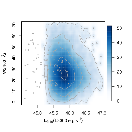
Figure 2: A plot of $W2400$ against $\log_{10}L3000$ for the sample dr7qso10. $L3000$ is the intrinsic continuum flux, in units of erg s^-1, at 3000 Å in the rest frame (see the text for its definition). The shading indicates the kernel-smoothed densities of points in a $64\times 64$ grid, because the number of points, 25700, is too high for an ordinary scatterplot to be a useful illustration. Linear contours for the densities are also shown. The plot has been restricted to $44.6\leq log_{10}L3000\leq 47.0$ and $0\leq W2400\leq 70$ Å for clarity. Note that the highest Fe II emitters tend to favour lower values of $\log_{10}L3000$. The plot also shows, as points (crosses), $W2400$ against $\log_{10}L3000$, for the sample sfqs10 (80 quasars). The same trend is apparent for the sfqs10 quasars.

This tendency of the highest Fe II emission favouring relatively low $\log_{10}L3000$ is further illustrated in Fig. 3, which shows, for the dr7qso10 sample, the distributions of $\log_{10}L3000$ for the 1531 ultrastrong emitters (solid histogram, blue online) and for the 7086 strong emitters (hatched histogram, red online). The difference in the distributions is very clear.

A one-sided Mann-Whitney test indicates that there is a shift to smaller values of $\log_{10}L3000$ for the ultrastrong emitters (1531 quasars) relative to the strong emitters (7086 quasars) at a level of significance given by a p-value of $1.260\times 10^{-12}$. The median shift is estimated as $0.046\pm 0.006$ in the logarithm, using the Hodges-Lehmann estimator (Hodges & Lehmann, 1963). In contrast, there is no relative shift in the distributions of $\log_{10}L3000$ for the two weaker intervals $20\leq W2400<30$ (weak_upper, 9845 quasars) and $10\leq W2400<20$ (weak_middle, 5871 quasars). They are indistinguishable (p-value of $0.504$).

These and other results in this section from our applications of the one-sided Mann-Whitney test are summarised in Table LABEL:mw_summary_table. Note that we have avoided comparisons with the interval weak_lower because the measurements of $W2400$ there can become comparable to the indicative errors.

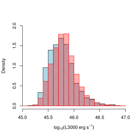
Figure 3: The distributions of $\log_{10}L3000$ for the 1531 ultrastrong $W2400$ emitters of the dr7qso10 sample (solid histogram, blue online) and for the 7086 strong $W2400$ emitters (hatched histogram, red online). $L3000$ is the intrinsic continuum flux, in units of erg s^-1, at 3000 Å in the rest frame (see the text for its definition). Both are density histograms. The bin size is 0.1 in the logarithm. The histograms have been restricted to $45.0\leq log_{10}L3000\leq 47.0$ Å for clarity. The distribution for the ultrastrong emitters is clearly shifted to lower values of $\log_{10}L3000$ relative to that for the strong emitters.

Similarly, for the smaller but generally lower-luminosity sample sfqs10, a one-sided Mann-Whitney test indicates that there is a shift to smaller values of $\log_{10}L3000$ for the ultrastrong emitters (12 quasars) relative to the strong emitters (30 quasars) at a level of significance given by a p-value of $3.545\times 10^{-4}$. The median shift is estimated as $0.376\pm 0.093$ in the logarithm. Similarly, again, there is no relative shift in the distributions of $\log_{10}L3000$ for the two weaker intervals $20\leq W2400<30$ (weak_upper, 17 quasars) and $10\leq W2400<20$ (weak_middle, 15 quasars). They are again indistinguishable (p-value of $0.892$).

Note that this trend for $W2400$ to increase as $L3000$ (or $\log_{10}L3000$) decreases is not strictly a correlation — it does not exist across the entire range of $W2400$ and $\log_{10}L3000$. From the large dr7qso10 sample, the trend exists for $W2400\ga 25$ Å, but $W2400$ appears to be essentially independent of $\log_{10}L3000$ for $W2400\la 25$ Å — see again the contours in Fig. 2. The observed trend should therefore not be confused with a Baldwin effect.

If we consider the quasars from dr7qso10 that are members of LQGs and, as in Clo13b, consider in particular, the range $1.1\leq\bar{z}_{LQG}\leq 1.5$ then, from the one-sided Mann-Whitney test, we find a stronger shift — $0.103\pm 0.015$ in the logarithm — to smaller values of $\log_{10}L3000$ for the ultrastrong emitters (120 quasars) relative to the strong emitters (463 quasars), at a level of significance given by a p-value of $2.024\times 10^{-9}$. (Compare with the shift of $0.046\pm 0.006$ obtained above for dr7qso10 quasars in general.) Here too, there is no relative shift in the distributions of $\log_{10}L3000$ for the two weaker intervals weak_upper and weak_middle (Table LABEL:mw_summary_table).

The LQGs are as defined in Clo13b, but here we are using only those members that are also from dr7qso10. Recall that dr7qso10 has the criterion $sn\_med\geq 10.0$, which is needed here because, unlike Clo13b, we are not making (and cannot make) comparisons with matched control samples.

If we consider the quasars from dr7qso10 that are not members of LQGs then we find a shift to smaller values of $\log_{10}L3000$ of $0.042\pm 0.006$ for the ultrastrong emitters relative to the strong emitters (Table LABEL:mw_summary_table), which is comparable to the shift ($0.046\pm 0.006$) for the dr7qso10 quasars in general, since LQG members constitute only a small fraction of the total ($\sim$ 11 per cent). Again, there is no relative shift for weak_upper and weak_middle (Table LABEL:mw_summary_table).

We now briefly summarise the results so far. We find that for quasars in general the highest Fe II emission, measured by $W2400$, tends to be associated with the lowest intrinsic continuum fluxes, measured by $L3000$, and expressed as $\log_{10}L3000$. We refer to this as the universal dependence, because it applies to quasars in general. This tendency for $W2400$ to increase as $\log_{10}L3000$ decreases is not strictly a correlation (so not a Baldwin effect) as it appears to take effect only for $W2400\ga 25$ Å. In accord with Clo13b, there appears to be a further, differential, dependence for those quasars that are members of LQGs, especially those with $1.1\leq z_{LQG}\leq 1.5$, corresponding to a more marked shift of the highest $W2400$ to lower values of $\log_{10}L3000$.

We can illustrate further the universal dependence in Fig. 4, which shows the distributions of $W2400$ of the samples sfqs10 and dr7qso10, corresponding to Fig. 2. The sample sfqs10 is generally of lower luminosity than dr7qso10, and its relative preponderance of strong and ultrastrong values of $W2400$ is very clear in the Figure.

Figure 4: The distributions of the rest-frame equivalent width, $W2400$, for the 80 quasars (from 83) of the sample sfqs10 (solid histogram, blue online) and for the 25700 quasars (from 25742) of the sample dr7qso10 (hatched histogram, red online). (Recall that for the 80 and the 25700 we can measure all of $W2400$, $fwhm2798$, and $L3000$.) Both are density histograms. The bin size is 5 Å. The histograms have been restricted to $0\leq W2400\leq 70$ Å for clarity. The universal dependence — the tendency of the highest Fe II $W2400$ emission to be associated with the lowest intrinsic continuum luminosities — is clearly seen as the relative preponderance of strong and ultrastrong emitters for the generally lower-luminosity sample sfqs10.

3.1.1 BALs in sfqs10

A higher rate of BALs for faint quasars compared with brighter quasars could conceivably introduce some component of the shift to stronger $W2400$ values. We have examined the spectra of the 55 sfqs10 quasars with $\log_{10}L3000\leq 45.4$ that contribute to Fig. 4 and Fig. 2 to judge whether there is any indication of an unusually high frequency of BALs. Recall that the sfqs10 quasars are generally lower-luminosity quasars — see Fig. 2.

We find no occurrences of the relatively rare, low-ionisation Mg II troughs in the spectra of these 55 quasars. However, high-ionisation C IV $\lambda 1549$ troughs would not be detectable in the spectra of those sfqs10 quasars that have $z\la 1.5$. For C IV BALs we are therefore limited to considering only those sfqs10 spectra for which $z\ga 1.5$: 13 from the 55 have $z\geq 1.50$. Of these 13, one, at $z=1.64$, appears very likely to be a BAL; it has $W2400=43.2$ Å, which is in the strong category, but close to being in the ultrastrong. Two of the 13 quasars have higher values of $W2400$, both in the ultrastrong category: one is clearly not a BAL; the other is almost certainly not a BAL, but its redshift is close to the limit for detection. Consequently, although the opportunities here to recognise BALs are evidently few, there is at least no reason to suppose that for $z\geq 1.50$ the frequency and properties of BAL quasars are different from those at brighter continuum luminosities. We shall assume that the same applies also to $z\la 1.5$.

3.2 ${\bf W2400}$ and line-widths

We have previously suspected that ultrastrong UV Fe II emission tends to be associated with quasars that have broad emission lines that are unusually narrow.

We can therefore perhaps gain some understanding of the universal dependence of the $W2400$ emission on $L3000$ and the differential dependence for the members of LQGs by considering Fig. 5. It plots $W2400$ against $fwhm2798$, the FWHM of the Mg II $\lambda 2798$ emission (calculated as described in section 2), for the sample dr7qso10. Recall that dr7qso10 specifies: $1.0\leq z\leq 1.8$, $i\leq 19.1$, and $sn\_med\geq 10.0$; it has 25742 quasars. We can measure all of $W2400$, $fwhm2798$, and $L3000$ for 25700 of the dr7qso10 quasars. The number of points is too high for an ordinary scatterplot to be a useful illustration and so the plot shows instead the kernel-smoothed densities of points in a $64\times 64$ grid. Note that the highest Fe II emitters tend to favour relatively narrow Mg II emission lines. It is not an exclusive relation however: high Fe II emission does not guarantee narrow Mg II, and narrow Mg II emission does not guarantee high Fe II emission.

This tendency of the highest Fe II emission favouring relatively narrow Mg II emission is further illustrated in Fig. 6, which shows, for the dr7qso10 sample, the distributions of $fwhm2798$ for the 1531 ultrastrong emitters (solid histogram, blue online) and for the 7086 strong emitters (hatched histogram, red online). Of course, the boundary between strong and ultrastrong is somewhat arbitrary, but the difference in the distributions is nevertheless very clear.

A one-sided Mann-Whitney test indicates that there is a relative shift to smaller values of the $fwhm2798$ distribution for the ultrastrong emitters at a level of significance given by a p-value of $1.522\times 10^{-9}$. The median shift is estimated as $1.89\pm 0.28$ Å. A similar result is obtained if instead we use the FWHM_MGII parameter (whole profile — i.e. broad $+$ narrow) from Shen et al. (2011): p-value of $3.504\times 10^{-16}$ and median shift of $2.40\pm 0.26$ Å (for 1530 ultrastrong emitters and 7065 strong emitters here, since FWHM_MGII is available only for 25613 of the 25700 quasars).

The tendency is not detected with the sfqs10 sample (the 80 from 83 for which we can measure all of $W2400$, $fwhm2798$, and $L3000$) by applying the Mann-Whitney test to the ultrastrong (12 quasars) and strong emitters (30 quasars), and so it is presumably less marked than the effect for $\log_{10}L3000$. Nevertheless, we can note the consistency of this tendency with the properties of the sfqs10 sample: 23 of the 42 quasars (55 per cent) that are ultrastrong or strong emitters have narrow $fwhm2798<35.0$ Å, whereas only 13 of the 38 quasars (34 per cent) that are weak emitters have $fwhm2798<35.0$ Å.

Figure 5: A plot of $W2400$ against $fwhm2798$, the FWHM of the Mg II $\lambda 2798$, emission for the sample dr7qso10. The shading indicates the kernel-smoothed densities of points in a $64\times 64$ grid, because the number of points, 25700, is too high for an ordinary scatterplot to be a useful illustration. The plot has been restricted to $0\leq fwhm2798\leq 140$ Å and $0\leq W2400\leq 70$ Å for clarity. Note that the highest Fe II emitters tend to favour relatively narrow Mg II emission lines.

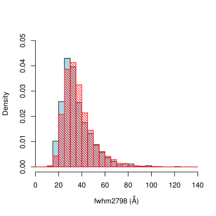
Figure 6: The distributions of the FWHM, $fwhm2798$, of the Mg II emission line for the 1531 ultrastrong $W2400$ emitters of the dr7qso10 sample (solid histogram, blue online) and for the 7086 strong $W2400$ emitters (hatched histogram, red online). Both are density histograms. The bin size is 5 Å. The histograms have been restricted to $0\leq fwhm2798\leq 140$ Å for clarity. The tendency of the highest Fe II emission to favour relatively narrow Mg II emission is clearly seen.

Although we do not show it here, the tendency for $W2798$ is different: higher $W2798$ tends to favour broader $fwhm2798$, as found also by Shen et al. (2011). If we assume that the Fe II emission and the Mg II line arise from the same locations within the BLR then, presumably, any hypothetical orientation effects of the flattened BLR would be identical. In that case, we can suspect a direct connection between narrow $fwhm2798$ and enhanced $W2400$. Narrow (BLR) Mg II line emission presumably corresponds to narrow (BLR) Ly$\alpha$ emission. (The widths of Mg II and Ly$\alpha$ are presumably both determined by the mass of the central BH, but are unlikely to be identical because of stratification, Ly$\alpha$ absorption, Ly$\alpha$ blending with N V $\lambda 1240$, and other factors.) We have few opportunities to test such a correspondence because Ly$\alpha$ will be in the ultraviolet region when Mg II and Fe II are observed in the optical region. However, from our own data, we do have GALEX ultraviolet spectra for a few of the quasars for which we have optical MMT / Hectospec spectra (see Appendix A). In Fig. 7 we show the GALEX ultraviolet spectra, converted to rest-frame wavelengths, for the ultrastrong emitters qso412 and qso425, for which we previously showed optical spectra, converted to rest-frame wavelengths, in Fig. 1. Clearly, qso412 has broad Mg II line emission, and qso425 has narrow Mg II line emission. Clearly, Ly$\alpha$ is correspondingly broad for qso412 and correspondingly narrow for qso425. For Ly$\alpha$ the ratio of FWHMs, qso412 : qso425, is 1.6 (from 24.4 Å and 15.7 Å), and for Mg II it is 2.1 (from 50.6 Å and 24.2 Å). See Appendix A for further details. Also, note again what we emphasised above: the tendency of the highest Fe II emitters favouring relatively narrow Mg II emission does not exclude the occurrence of quasars such as qso412 with ultrastrong $W2400$ and broad Mg II.

Figure 7: Rest-frame (ultraviolet) spectra of two ultrastrong UV Fe II-emitting quasars, qso412 ($z=1.156$) and qso425 ($z=1.230$), from our GALEX spectra (Appendix A). The rest-frame optical spectrum (Fig. 1) shows broad Mg II $\lambda 2798$ line emission for qso412, and narrow for qso425. Here it can be seen that the Ly$\alpha$ $\lambda 1216$ line emission is correspondingly broad for qso412 and narrow for qso425. The spectra have been smoothed with a 5-pixel median filter. The flux densities ($f_{\lambda}$) are in units of $10^{-16}$ erg s^-1 cm^-2 Å^-1. The wavelength range has been restricted to $\sim$ 950–1250 Å for clarity. See Table LABEL:mmt_hecto_quasars for further details of these two quasars.

For a given Ly$\alpha$ flux, a narrow line will concentrate relatively more flux than a broad line in the region Ly$\alpha$ $\lambda 1216$ $\pm 3$ Å (Johansson & Jordan, 1984; Sigut & Pradhan, 1998) that is most important for Ly$\alpha$ fluorescence of the UV Fe II. We suggest, therefore, that Ly$\alpha$ fluorescence might be in large part responsible for both the universal dependence of $W2400$ on $L3000$ and the differential dependence for LQG members.

We mentioned previously that, for Ly$\alpha$ fluorescence, the ratio of FWHM to equivalent width of the Ly$\alpha$ would be a useful central-concentration parameter for associating with the Fe II emission. For the spectral coverage of our quasar data we cannot routinely calculate this ratio for Ly$\alpha$, which then falls in the ultraviolet region. Perhaps, however, Mg II can be used as at least a rough guide to the ratio for Ly$\alpha$. In Fig. 8, we plot $W2400$ against $fwhm2798/W2798$ for dr7qso10. Again, the number of points (25700) is too high for an ordinary scatterplot to be a useful illustration and the plot shows instead the kernel-smoothed densities of points in a $64\times 64$ grid. Note that increasing $W2400$ emission seems to be associated with decreasing values of the ratio $fwhm2798/W2798$. That is, increasingly strong UV Fe II emission does seem to be associated with increasingly centrally-concentrated Mg II emission at least. Note again, of course, that the Mg II emission can be affected by Fe II emission, especially on the blueward side.

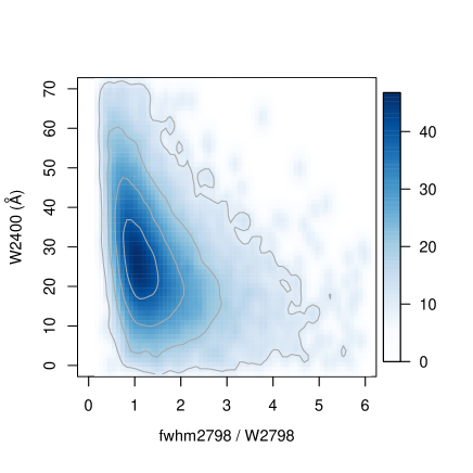
Figure 8: A plot of $W2400$ against $fwhm2798/W2798$, the FWHM of the Mg II $\lambda 2798$ emission divided by the equivalent width, for the sample dr7qso10. The shading indicates the kernel-smoothed densities of points in a $64\times 64$ grid, because the number of points, 25700, is too high for an ordinary scatterplot to be a useful illustration. The plot has been restricted to $0\leq fwhm2798/w2798\leq 6.0$ and $0\leq W2400\leq 70$ Å for clarity. Note that increasing $W2400$ emission seems to be associated with decreasing values of the ratio $fwhm2798/W2798$.

3.3 Interpretation

We might expect narrow emission lines to have some correspondence with relatively less massive central BHs — either to AGN that intrinsically have low BH masses or to younger quasars that are still growing their central BHs and have not yet reached their mature state (e.g. Mathur, 2000). In Fig. 9, we plot $W2400$ against $\log_{10}(M_{\rm BH}/M_{\odot})$ for dr7qso10, where $M_{\rm BH}$ is the adopted “fiducial” virial BH mass from Shen et al. (2011). $M_{\rm BH}$ is actually determined by a FWHM, acting as a proxy for virial velocity, and by a continuum luminosity, acting as a proxy for BLR radius. Again, the number of points (25670 of the previous 25700 have a measurement of $M_{\rm BH}$) is too high for an ordinary scatterplot to be a useful illustration and the plot shows instead the kernel-smoothed densities of points in a $64\times 64$ grid. From Shen et al. typical errors in the BH masses, propagated from the measurement uncertainties in the continuum luminosities and the FWHMs, are $\sim$ 0.05–0.2 dex, but the additional statistical uncertainty in the calibration of virial masses is $\sim$ 0.3–0.4 dex. Nevertheless, there does appear to be a trend in Fig. 9, with average ultrastrong emitters having smaller BH masses than average weak emitters by a factor of $\sim 2$. Clearly, the ultrastrong emitters are not in the low-BH-mass category ($\la 10^{8}M_{\odot}$) of AGN, and we might instead expect that they are still growing their BHs. In that case, increasing $W2400$ emission would have an association with increasingly young quasars. We further suggest that this possible interpretation in terms of younger quasars helps to clarify the nature of LQGs. LQGs — regions with an overdensity of quasars — would then be interpreted quite naturally as regions that contain a higher proportion of young quasars than field regions.

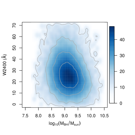
Figure 9: A plot of $W2400$ against $\log_{10}(M_{\rm BH}/M_{\odot})$, where $M_{\rm BH}$ is the adopted “fiducial” virial BH mass from Shen et al. (2011), for the sample dr7qso10. The shading indicates the kernel-smoothed densities of points in a $64\times 64$ grid, because the number of points, 25670, is too high for an ordinary scatterplot to be a useful illustration. The plot has been restricted to $7.5\leq\log_{10}(M_{\rm BH}/M_{\odot})\leq 10.5$ and $0\leq W2400\leq 70$ Å for clarity. Note that increasing $W2400$ emission seems to be associated with decreasing values of $M_{\rm BH}$.

4 Further notes

In this section we make some further notes on the content of the paper, some of which have a slightly cautionary nature because of the possibilities of small systematic biases in the measurements and because of the difficulty of clarifying further the possible implications of the data.

First of all, we note that there is a correlation of $W2400$ with $W2400g$ (Fig. 10). Recall from section 2 that $W2400g$ is a measure of the gradient of the line taken as the continuum in the Weymann et al. (1991) definition of the equivalent width $W2400$. It is represented as a colour. A similar correlation results if instead of $W2400g$ we use the similarly-defined continuum colour $-2.5\log_{10}[(L2200/2200)/(L3000/3000)]$, which corresponds to a larger interval of wavelength than $W2400g$. The correlations are presumably counterparts of correlations with spectral index.

In connection with Fig. 1, in section 2, we discussed briefly the effect of artificially changing the curvature of the spectrum of qso412 to resemble that of qso425. It reduced $W2400$ from 55.5 Å to 52.1 Å, the difference of 3.4 Å being comparable to the indicative measurement errors. Similarly, for dr7qso10, we find that $W2400$ for the red quasars ($W2400g>0$, 1292 from 25700 — so only $\sim$ 5 per cent of the total) in Fig. 10 could be biased with respect to $W2400$ for the blue quasars by $\sim 3$ Å. If so, the correlation might then be exaggerated by a small bias in $W2400$ for red quasars with respect to blue but cannot be attributed to it. However, by artificially changing the curvature of the spectra we are clearly also changing the quasars (from red to blue): it may be that the measurements of $W2400$ for the red quasars are mostly legitimate, and not subject to any such small bias.

The $1/\lambda$ function by which we artificially change the curvature of a spectrum (here and as mentioned in section 2) is this: first, we multiply by a function of $1/\lambda$ such that $f_{\lambda}(3000)$ is unchanged and $f_{\lambda}(1900)$ is doubled; then we scale the spectrum such that the median flux density across 2255‒-2650 Å is unchanged.

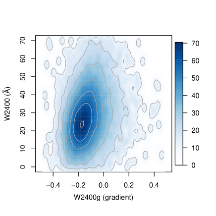
Figure 10: A plot of $W2400$ against $W2400g$, a measure of the gradient, represented as a colour, of the line taken as the continuum in the Weymann et al. (1991) definition of the equivalent width $W2400$, for the sample dr7qso10. The shading indicates the kernel-smoothed densities of points in a $64\times 64$ grid, because the number of points, 25700, is too high for an ordinary scatterplot to be a useful illustration. The plot has been restricted to $-0.5\leq W2400g\leq 0.5$ and $0\leq W2400\leq 70$ Å for clarity. Note the clear correlation, which might be exaggerated by a small bias in $W2400$ for red quasars with respect to blue, but which cannot be attributed to it.

We mentioned previously, in a footnote, that we have reasons to prefer our measure $W2400$ to the UV EW Fe ($EW\_FE\_MGII$) measure from template-fitting of Shen et al. (2011). Nevertheless, we note that their measure also correlates with $W2400g$ and with the continuum colour $-2.5\log_{10}[(L2200/2200)/(L3000/3000)]$, although the trends with their measure have more complexity or internal structure.

This dependence of $W2400$ on $W2400g$ and on the similar measure of continuum colour $-2.5\log_{10}[(L2200/2200)/(L3000/3000)]$ (and similarly for the Shen et al. UV EW Fe measure) thus appears to be a small dependence of the UV Fe on continuum colour. Note that it does not appear to arise from the dependence of $W2400$ on $L3000$ that we find (section 3.1): $W2400g$ appears to be only slightly dependent on $L3000$ — see Fig. 11, which plots $W2400g$ against $\log_{10}L3000$ as kernel-smoothed densities for the sample dr7qso10 and as points for the sample sfqs10. For illustration, the Mann-Whitney test applied to the dr7qso10 data, shows that there is a significant (p-value $<2.2\times 10^{-16}$) but small dependence of $W2400g$ on $\log_{10}L3000$ –— corresponding to a colour shift of only $\Delta(W2400g)\sim 0.025\pm 0.002$ for the interval $45.4\leq\log_{10}L3000<45.5$ compared with the interval $45.9\leq\log_{10}L3000\leq 46.0$. Of course our finding that stronger $W2400$ tends to be associated with fainter $L3000$ combined with the correlation of $W2400$ and $W2400g$ means that there must be some tendency, even if small, for $W2400g$ to be redder for fainter $L3000$.

We note that the modelling by Verner et al. (2003), Verner et al. (2004) and Bruhweiler & Verner (2008) appears to take spectral index as a fixed quantity rather than a variable. Bruhweiler & Verner (2008) do, however, mention that the shape of the spectral energy distribution would be a consideration in future work, although we have not found any subsequent references in which it is considered.

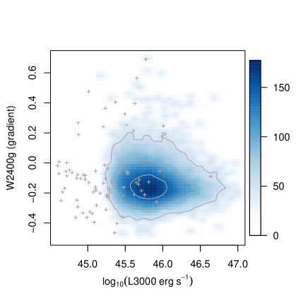
Figure 11: A plot of $W2400g$ against $\log_{10}L3000$ for the sample dr7qso10. $L3000$ is the intrinsic continuum flux, in units of erg s^-1, at 3000 Å in the rest frame (see the text for its definition). $W2400g$ is a measure of the gradient, represented as a colour, of the line taken as the continuum in the Weymann et al. (1991) definition of the equivalent width $W2400$. The shading indicates the kernel-smoothed densities of points in a $64\times 64$ grid, because the number of points, 25700, is too high for an ordinary scatterplot to be a useful illustration. Linear contours for the densities are also shown. The plot has been restricted to $44.6\leq log_{10}L3000\leq 47.0$ and $-0.5\leq W2400g\leq 0.7$ for clarity. The plot also shows, as points (crosses), $W2400g$ against $\log_{10}L3000$, for the sample sfqs10 (80 quasars). Note that $W2400g$ appears to be only slightly dependent on $\log_{10}L3000$.

5 Conclusions

The conclusions of this paper are the following.

1. We find that for $W2400\ga 25$ Å there is a universal (i.e. for quasars in general) strengthening of $W2400$ with decreasing intrinsic luminosity, $L3000$.

2. In conjunction with the work presented by Clowes et al. (2013b), we find that there is a further, differential, strengthening of $W2400$ with decreasing $L3000$ for those quasars that are members of Large Quasar Groups, or LQGs.

3. We find that increasingly strong $W2400$ tends to be associated with decreasing FWHM of the neighbouring Mg II $\lambda 2798$ broad emission line.

4. On the assumption that this trend that $W2400$ increases as the FWHM of Mg II decreases is true also for the FWHM of the Ly$\alpha$ emission line, we suggest that this dependence of $W2400$ on intrinsic luminosity arises from Ly$\alpha$ fluorescence. We make this suggestion because: the wavelength region $1216\pm 3$ Å is important for Ly$\alpha$ fluorescence of the Fe II emission; for a given Ly$\alpha$ equivalent width, narrower Ly$\alpha$ emission would enhance the flux in this region, and hence fluorescence of the Fe II, relative to broader Ly$\alpha$ emission.

5. We find that stronger $W2400$ tends to be associated with smaller virial estimates of the mass of the central black hole, by a factor $\sim 2$ between the ultrastrong emitters (smaller black holes) and the weak. The effect for $W2400$ can then be associated with a range of masses for the central black holes. Stronger $W2400$ emission would correspond to smaller black holes that are still growing. They will be in fainter quasars, with relatively narrow broad-emission lines, leading to the enhanced Ly$\alpha$ fluorescence of the UV Fe II emission. The differential effect for LQGs might then arise from a different mass distribution of the black holes, corresponding, plausibly, to an age distribution that emphasises younger quasars in the LQG environments.

6 Acknowledgments

We wish to thank: Linhua Jiang for providing us with the SFQS spectra in digital form; and Martin Gaskell for very informative discussions on the characteristics of the BLRs in quasars.

The anonymous referee is thanked for a thoughtful and constructive review of the paper.

We also wish to thank the R Foundation for Statistical Computing for the R software.

LEC received partial support from the Center of Excellence in Astrophysics and Associated Technologies (PFB 06), and from a CONICYT Anillo project (ACT 1122).

SR was in receipt of a CONICYT PhD studentship while much of this work was in progress.

This research has used the SDSS DR7QSO catalogue (Schneider et al., 2010).

Funding for the SDSS and SDSS-II has been provided by the Alfred P. Sloan Foundation, the Participating Institutions, the National Science Foundation, the U.S. Department of Energy, the National Aeronautics and Space Administration, the Japanese Monbukagakusho, the Max Planck Society, and the Higher Education Funding Council for England. The SDSS Web Site is http://www.sdss.org/.

The SDSS is managed by the Astrophysical Research Consortium for the Participating Institutions. The Participating Institutions are the American Museum of Natural History, Astrophysical Institute Potsdam, University of Basel, University of Cambridge, Case Western Reserve University, University of Chicago, Drexel University, Fermilab, the Institute for Advanced Study, the Japan Participation Group, Johns Hopkins University, the Joint Institute for Nuclear Astrophysics, the Kavli Institute for Particle Astrophysics and Cosmology, the Korean Scientist Group, the Chinese Academy of Sciences (LAMOST), Los Alamos National Laboratory, the Max-Planck-Institute for Astronomy (MPIA), the Max-Planck-Institute for Astrophysics (MPA), New Mexico State University, Ohio State University, University of Pittsburgh, University of Portsmouth, Princeton University, the United States Naval Observatory, and the University of Washington.

Appendix A MMT / Hectospec and GALEX data

In this paper we have made a little use of our own MMT / Hectospec spectra and GALEX spectra. We give here some more details, especially for the MMT / Hectospec spectra. Table LABEL:mmt_hecto_quasars gives our measurements of $W2400$ and other parameters from these MMT / Hectospec spectra, primarily for the redshift range $1.0\leq z\leq 1.8$, but, for completeness, with some information for the quasars outside this range included too.

The MMT / Hectospec spectra were obtained in 1.6 deg² from two adjacent $0.8~{}{\rm deg}^{2}$ Hectospec fields. The fields intersect the LQGs U1.11, U1.28, and U1.54 (Clowes et al., 2012; Clowes & Campusano, 1991), with the last of these being the “doubtful LQG” (a previously published LQG, but one of marginal significance in our catalogue). Quasars in the redshift range $1.0\leq z\leq 1.8$ are of particular interest to us, because this is the range corresponding to our main DR7QSO catalogue of LQGs.

The RA, Dec (2000) field centres were approximately: 10:48:40.8, $+$05:24:36 ($162.17\degr,5.41\degr$) and 10:50:04.8, $+$04:31:12 ($162.52\degr,4.52\degr$), but some small adjustments were made during the observations across two months. Spectra were obtained during February and April 2010, covering 3650–9200 Å at $\sim$ 6 Å resolution, with integration times typically 5400 s but with some variation. As mentioned previously, we used the wavelength range 3900–8200 Å in the measurement of $W2400$ and other parameters from our MMT / Hectospec spectra. Also as mentioned previously, for our MMT / Hectospec spectra only, the atmospheric A-band at $\sim$ 7600 Å is prominent and we have interpolated across it. For the redshift range $1.0\leq z\leq 1.8$ the measurements of $W2400$ do not contain the interpolation. For two of these quasars, noted in Table LABEL:mmt_hecto_quasars, the Mg II emission does contain the interpolation and the measurements of $fwhm2798$ could be affected a little. For three quasars outside the range $1.0\leq z\leq 1.8$ the measurements of $W2400$ do contain the interpolation, and these too have been noted in Table LABEL:mmt_hecto_quasars.

The MMT / Hectospec observations of the quasars were “fibre-filling” observations — using spare fibres after the objects for the main programme (on galaxies) had all been allocated fibres. The quasar candidates that were selected for observation were drawn from a list that had been prepared previously using the SDSS DR1 photometric quasar catalogue of Richards et al. (2004). All of the candidates in the list were selected to have $18.0\leq r\leq 21.2$ (the catalogue itself was defined by $g\leq 21$). The candidates chosen from the list for the fibre-filling emphasised first $z_{\rm phot}=$ 0.7–0.9, 1.2–1.4, then $z_{\rm phot}=$ 0.6–0.7, 0.9–1.2, 1.4–1.5, followed by any other $z_{\rm phot}$ values. However, the later DR6 photometric quasar catalogue of Richards et al. (2009) revised the photometric redshifts, sometimes substantially, and these criteria will have become blurred. In retrospect, from the MMT / Hectospec spectroscopic redshifts, the net effect seems to be that the fibre-filling selected candidates typically with $z\sim$ 1.0–2.3 (90 per cent) and a few with $z\sim$ 0.6–0.7 (10 per cent).

The MMT / Hectospec observations resulted in spectra for 31 quasars, with redshifts in the range 0.613–2.228, and $g$ in the range 18.486–20.955. Of these 31, 21 have $1.0\leq z\leq 1.8$; these 21 have $g$ in the range 18.486–20.947. Note that we have taken magnitudes of the MMT / Hectospec quasars from the later DR6 photometric quasar catalogue (Richards et al., 2009). One of the quasars is seen to be a BAL quasar ($W2400=38.4$ Å, strong). Six of these 31 are also contained in the DR7QSO catalogue.

Accurate spectrophotometric calibration was not a particular concern of the MMT / Hectospec observations and errors of $\la$ 20 per cent are expected, with the values of $L3000$ and hence log₁₀L3000 (Table LABEL:mmt_hecto_quasars) affected correspondingly.

We note the consistency of the data in Table LABEL:mmt_hecto_quasars with the tendency of the strongest Fe II emitters to be associated with relatively narrow Mg II emission. For $1.0\leq z\leq 1.8$ and $sn\_med\geq 10.0$, 9 of the 12 quasars (75 per cent) that are ultrastrong or strong emitters have narrow $fwhm2798<35.0$ Å, whereas only 2 of the 6 quasars (33 per cent) that are weak emitters (and with Mg II unaffected by the A-band) have $fwhm2798<35.0$ Å.

We have also made a little use of ultraviolet spectra from GALEX. These spectra were obtained in parallel with a main programme of imaging from GALEX within the two MMT / Hectospec fields. The GALEX fields and the MMT / Hectospec fields are essentially the same. The GALEX spectra are slitless, in the far-UV (FUV), $\sim$ 1350–1800 Å, and the near-UV (NUV), $\sim$ 1800–2800 Å. The point-source resolutions are $\sim$ 10 Å and $\sim$ 25 Å respectively. Extraction of the spectra was done by GALEX staff. GALEX procedures circumvent overlapped spectra by observing a field with a series of grism-angle rotations relative to the sky. There can be problems of second-order and third-order overlaps in the FUV affecting the brighter and bluer objects. We have GALEX spectra for 11 of the MMT / Hectospec quasars listed in Table LABEL:mmt_hecto_quasars. Of these 11, five provide usable spectra across the Ly$\alpha$ region. Two of these five happened to have ultrastrong $W2400$; we used their spectra in Fig. 7, together with the corresponding optical spectra in Fig. 1, to illustrate the plausibility of broad / narrow Ly$\alpha$ corresponding to broad / narrow Mg II. The other three have Ly$\alpha$ and Mg II widths that correspond similarly.

References

- Baldwin (1977) Baldwin J.A., 1977, ApJ, 214, 679
- Baldwin et al. (1995) Baldwin J., Ferland G., Korista K., Verner D., 1995, ApJ, 455, L119
- Baldwin et al. (2004) Baldwin J.A., Ferland G.J., Korista K.T., Hamann F., LaCluyzé A., 2004, ApJ, 615, 610
- Barth et al. (2013) Barth A.J. et al., 2013, ApJ, 769:128
- Baskin (2012) Baskin A., 2012, in Chartas G., Hamann F., Leighly K.M., eds, AGN Winds in Charleston. ASP Conf. Ser. 460, ASP, San Francisco, p. 159
- Baskin & Laor (2012) Baskin A., Laor A., 2012, MNRAS, 426, 1144
- Baskin et al. ( 2014) Baskin A., Laor A., Stern J., 2014, MNRAS, 438, 604
- Bian et al. (2012) Bian W.-H., Fang L.-L., Huang K.-L., Wang J.-M., 2012, MNRAS, 427, 2881
- Bottorff & Ferland (2001) Bottorff M., Ferland G., 2001, ApJ, 549, 118
- Bottorff et al. (2000) Bottorff M., Ferland G., Baldwin J., Korista K., 2000, ApJ, 542, 644
- Bruhweiler & Verner (2008) Bruhweiler F., Verner E., 2008, ApJ, 675, 83
- Cackett et al. (2015) Cackett E.M., Gültekin K., Bentz M.C., Fausnaugh M.M., Peterson B.M., Troyer J., Vestergaard M., 2015, ApJ, 810:86
- Clowes & Campusano (1991) Clowes R.G., Campusano L.E., 1991, MNRAS, 249, 218
- Clowes et al. (2012) Clowes R.G., Campusano L.E., Graham M.J., Söchting I.K., 2012, MNRAS, 419, 556
- Clowes et al. (2013a) Clowes R.G., Harris K.A., Raghunathan S., Campusano L.E., Söchting I.K., Graham M.J., 2013a, MNRAS, 429, 2910
- Clowes et al. (2013b) Clowes R.G., Raghunathan S., Söchting I.K., Graham M.J., Campusano L.E., 2013b, MNRAS, 433, 2467 (Clo13b)
- Collin-Souffrin & Lasota (1988) Collin-Souffrin S., Lasota J.-P., 1988, PASP, 100, 1041
- Croom et al. (2009) Croom S.M. et al., 2009, MNRAS, 392, 19
- Czerny & Hryniewicz (2011) Czerny B., Hryniewicz K., 2011, A&A, 525, L8
- DeGroot & Schervish (2012) DeGroot M.H., Schervish M.J., 2012, Probability and Statistics, 4th ed., Pearson, Boston
- De Rosa et al. (2011) De Rosa G., Decarli R., Walter F., Fan X., Jiang L., Kurk J., Pasquali A., Rix H.W., 2011, ApJ, 739, 56
- Dietrich et al. (1999) Dietrich M., Wagner S.J., Courvoisier T.J.-L., Bock H., North P., 1999, A&A, 351, 31
- Dietrich et al. (2002) Dietrich M., Hamann F., Shields J.C., Constantin A., Vestergaard M., Chaffee F., Foltz C.B., Junkkarinen V.T., 2002, ApJ, 581, 912
- Dietrich et al. (2003) Dietrich M., Hamann F., Appenzeller I., Vestergaard M., 2003, ApJ, 596, 817
- Dolan et al. (2000) Dolan J.F., Michalitsianos A.G., Nguyen Q.T., Hill R.J., 2000, ApJ, 539, 111
- Draine (1989) Draine B.T., 1989, in Allamandola L.J., Tielens A.G.G.M., eds, Proc. IAU Symp. 135, Interstellar Dust. Kluwer, Dordrecht, p. 313
- Draine (2003) Draine B.T., 2003, ApJ, 598, 1017
- Gaskell (2009) Gaskell C.M., 2009, NewAR, 53, 140
- Gaskell & Goosmann (2013) Gaskell C.M., Goosmann R.W., 2013, ApJ, 769:30
- Goad & Korista (2015) Goad M.R., Korista K.T., 2015, MNRAS, 453, 3662
- (31) Goad M.R., Korista K.T., Ruff A.J., 2012, MNRAS, 426, 3086
- (32) Graham M.J., Clowes R.G., Campusano L.E., 1996, MNRAS, 279, 1349
- (33) Green P.J., Forster K., Kuraszkiewicz J., 2001, ApJ, 556, 727
- Grier et al. (2015) Grier C.J. et al., 2015, ApJ, 806:111
- Guerras et al. (2013) Guerras E., Mediavilla E., Jimenez-Vicente J., Kochanek C.S., Muñoz J.A., Falco E., Motta V., Rojas K., 2013, ApJ, 778:123
- Hamann & Ferland (1999) Hamann F., Ferland G., 1999, ARAA, 37, 487
- Hamann et al. (2004) Hamann F., Dietrich M., Sabra B.M., Warner C., 2004, in McWilliam A., Rauch M., eds, Origin and Evolution of the Elements, Carnegie Observatories Astrophysics Series Volume 4. CUP, p. 440
- Hartman & Johansson (2000) Hartman H., Johansson S., 2000, A&A, 359, 627
- Hecht (1986) Hecht J.H., 1986, ApJ, 305, 817 (with erratum, 1987, ApJ, 314, 429)
- Hodges & Lehmann (1963) Hodges J.L., Jr, Lehmann E.L., 1963, Ann. Math. Statist., 34, 598
- Hopkins et al. (2004) Hopkins P.F. et al., 2004, AJ, 128, 1112
- Jiang et al. (2006) Jiang L. et al., 2006, AJ, 131, 2788
- Jiang et al. (2010) Jiang P., Ge J., Prochaska J.X., Kulkarni V.P., Lu H.L., Zhou H.Y., 2010, ApJ, 720, 328
- Johansson & Jordan (1984) Johansson S., Jordan C., 1984, MNRAS, 210, 239
- Kishimoto et al. (2013) Kishimoto M. et al., 2013, ApJ, 775:L36
- Kollatschny & Zetl (2011) Kollatschny W., Zetl M., 2011, Nat, 470, 366
- Kollatschny & Zetl (2013) Kollatschny W., Zetl M., 2013, A&A, 558, A26
- Korista & Goad (2004) Korista K.T., Goad M.R., 2004, ApJ, 606, 749
- Kundić et al. (1997) Kundić T. et al., 1997, ApJ, 482, 75
- Leighly & Moore (2006) Leighly K.M., Moore J.R., 2006, ApJ, 644, 748
- Mathis (1990) Mathis J.S., 1990, ARAA, 28, 37
- Mathur (2000) Mathur S., 2000, MNRAS, 314, L17
- Matteucci & Recchi (2001) Matteucci F., Recchi S., 2001, ApJ, 558, 351
- Netzer (1980) Netzer H., 1980, ApJ, 236, 406
- (55) Nomoto K., Kobayashi C., Tominaga N., 2013, ARAA, 51, 457
- Noterdaeme et al. (2009) Noterdaeme P., Ledoux C., Srianand R., Petitjean P., Lopez S., 2009, A&A, 503, 765
- Pancoast et al. (2012) Pancoast A. et al., 2012, ApJ, 754:49
- Pancoast et al. (2014) Pancoast A., Brewer B.J., Treu T., Park D., Barth A.J., Bentz M.C., Woo J.-H., 2014, MNRAS, 445, 3073 (with erratum, 2015, MNRAS, 448, 3070)
- Pâris et al. (2014) Pâris I. et al., 2014, A&A, 563, A54
- Penston (1987) Penston M.V., 1987, MNRAS, 229, 1P
- Peterson (2006) Peterson B.M., 2006, in Alloin D., Johnson R., Lira P., eds, Physics of Active Galactic Nuclei at All Scales. Springer, Berlin, p. 77
- (62) Pitman K.M., Clayton G.C., Gordon K.D., 2000, PASP, 112, 537
- Reimers et al. (2005) Reimers D., Janknecht E., Fechner C., Agafonova I.I., Levshakov S.A., Lopez S., 2005, A&A, 435, 17
- Richards et al. (2004) Richards G.T. et al., 2004, ApJS, 155, 257
- Richards et al. (2006) Richards G.T. et al., 2006, AJ, 131, 2766
- Richards et al. (2009) Richards G.T. et al., 2009, ApJS, 180, 67
- Ruff et al. (2012) Ruff A.J., Floyd D.J.E., Webster R.L., Korista K.T., Landt H., 2012, ApJ, 754:18
- Sameshima et al. (2009) Sameshima H. et al., 2009, MNRAS, 395, 1087
- Schneider et al. (2010) Schneider D.P. et al., 2010, AJ, 139, 2360
- Schnülle et al. (2013) Schnülle K., Pott J.-U., Rix H.-W., Decarli R., Peterson B.M., Vacca W., 2013, A&A, 557, L13
- Shalyapin et al. (2008) Shalyapin V.N., Goicoechea L.J., Koptelova E., Ullán A., Gil-Merino R., 2008, A&A, 492, 401
- (72) Shalyapin V.N., Goicoechea L.J., Gil-Merino R., 2012, A&A, 540, A132
- Shen et al. (2008) Shen Y., Greene J.E., Strauss M.A., Richards G.T., Schneider D.P., 2008, ApJ, 680, 169
- Shen et al. (2011) Shen Y. et al., 2011, ApJS, 194:45
- Sigut & Pradhan (1998) Sigut T.A.A., Pradhan A.K., 1998, ApJ, 499, L139
- Sigut & Pradhan (2003) Sigut T.A.A., Pradhan A.K., 2003, ApJS, 145, 15
- Simon & Hamann (2010) Simon L.E., Hamann F., 2010, MNRAS, 407, 1826
- Vanden Berk et al. (2005) Vanden Berk D.E., et al., 2005, AJ, 129, 2047
- Verner et al. (2003) Verner E., Bruhweiler F., Verner D., Johansson S., Gull T., 2003, ApJ, 592, L59
- Verner et al. (2004) Verner E., Bruhweiler F., Verner D., Johansson S., Kallman T., Gull T., 2004, ApJ, 611, 780
- Verner et al. (2009) Verner E., Bruhweiler F., Johansson S., Peterson B., 2009, Phys. Scr. T134, 014006
- Vestergaard & Peterson (2005) Vestergaard M., Peterson B.M., 2005, ApJ, 625, 688
- Vestergaard & Wilkes (2001) Vestergaard M., Wilkes B.J., 2001, ApJS, 134, 1
- (84) Walsh D., Carswell R.F., Weymann R.J., 1979, Nat, 279, 381
- Weymann et al. (1991) Weymann R.J., Morris S.L., Foltz C.B., Hewett P.C., 1991, ApJ, 373, 23
- Wills & Browne (1986) Wills B.J., Browne I.W.A., 1986, ApJ, 302, 56
- Wills & Wills (1980) Wills B.J., Wills D., 1980, ApJ, 238, 1
- Wills et al. (1980) Wills B.J., Netzer H., Uomoto A.K., Wills D., 1980, ApJ, 237, 319
- (89) Wills B.J., Netzer H., Wills D., 1985, ApJ, 288, 94
- Young et al. (1980) Young P., Gunn J.E., Kristian J., Oke J.B., Westphal J.A., 1980, ApJ, 241, 507
- Young et al. (1981) Young P., Gunn J.E., Kristian J., Oke J.B., Westphal J.A., 1981, ApJ, 244, 736
- Zamorani et al. (1992) Zamorani G., Marano B., Mignoli M., Zitelli V., Boyle B.J., 1992, MNRAS, 256, 238
- Zhang et al. (2015) Zhang S. et al., 2015, ApJ, 802:92
- Zhang (2011) Zhang X.-G., 2011, ApJ, 741, 104