Comparison between cell-centered and nodal based discretization schemes for linear elasticity

Abstract.

In this paper we study newly developed methods for linear elasticity on polyhedral meshes. Our emphasis is on applications of the methods to geological models. Models of subsurface, and in particular sedimentary rocks, naturally lead to general polyhedral meshes. Numerical methods which can directly handle such representation are highly desirable. Many of the numerical challenges in simulation of subsurface applications come from the lack of robustness and accuracy of numerical methods in the case of highly distorted grids. In this paper we investigate and compare the Multi-Point Stress Approximation (MPSA) and the Virtual Element Method (VEM) with regards to grid features that are frequently seen in geological models and likely to lead to a lack of accuracy of the methods. In particular we look how the methods perform near the incompressible limit. This work shows that both methods are promising for flexible modeling of subsurface mechanics.

1. Introduction

Modeling of sedimentary subsurface rock naturally leads to general unstructured grids because of stratigraphic layering, erosion and faults. The industry standard for grids in reservoir modeling is the Corner-Point grids (cp-grids). Other geometrical grid formats have been proposed to improve on this format, but all compact representations of the underlying geology will lead to cells with high aspect ratios, distorted cells, large variations in cell volumes and faces areas. Methods that are valid on general polyhedral grids and are robust for different grid types will greatly simplify the modeling of subsurface physics for multiphase flow encountered in the oil and gas industry. The workhorse method there is the finite volume discretization based on a two point flux approximation (TPFA). The method is not convergent for general grids and can introduce large grid-orientation effects, see for example [13, Figure 3], but is very robust due to its monotonicity properties, which often result in faster computation times. The multi-point flux approximation (MPFA) method has been developed to solve the convergence problems and has been successfully applied to minimize grid-orientation effects [1, 10], but due to lack of monotonicity, the method is difficult to apply to complex grids such as those arising from real reservoir models. Based on a mixed formulation, the mimetic finite difference method has been proposed for incompressible flow [5, 4], but problems arise in the case of fully compressible black oil models, as the method introduces non-monotonicity and significantly more degrees of freedom. In recent years, coupling of geo-mechanical effects with subsurface flow has become more important in many areas including oil and gas production from mature fields, fractured tight reservoirs as well as geothermal application and risk assessment of CO2 injection. Realistic modeling of these geological cases is hampered by differences in the way geo-mechanics and flow models are built and discretized.

Recently, a cell-centered finite volume discretization has been proposed in [15] to specifically address problems arising in coupled geo-mechanical and flow simulation of porous media. The method is inspired from the MPFA discretization developed for flow problems and was thus named multi-point stress approximation (MPSA). The MPSA method presents two appealing features for subsurface applications. Since the method is based on the MPFA method, it shares the same data structure which is commonly used for the flow problem where the preferred methods remain based on finite volume discretization. Moreover, the method can operate on the type of general polyhedral grids typically used to represent complex heterogeneous medium. This later property is shared by the virtual element (VE) method [18]. The VE method builds upon the long-standing effort in the development of mimetic finite difference (MFD) methods, see [11, 19]. The MFD method reproduces at the discrete level fundamental properties of the differentiation operators, using only the available degrees of freedom and without explicitly constructing any finite element basis. In this way, the method can easily handle general cell shapes. The VE method is a reformulation of the MFD method in the finite element framework. As in the MFD method, a complete finite element basis for a polyhedral cell is not computed, some of the basis elements become virtual. Both the MPSA and the VE methods for mechanics naturally define the divergence of the displacement on cells (see [14] for MPSA), which is also the natural coupling term between flow and mechanics, when flow is discretized with finite volume methods. As pointed out in [15], any attempt to extend the TPFA method to mechanics is bound to fail as the method already fails the local patch test. The local patch test verifies that the numerical method preserves rigid rotations, which are exact solutions to the problem.

In this paper we will investigate the MPSA and VE methods for mechanics with special emphasis on grid artifacts that naturally occur in geological models of sedimentary. Even if both aspects are related, our first interest is not the convergence properties of the methods but their performance on coarse and distorted meshes. This paper contains the first set of tests where the MPSA method is tested in view of applications to geosciences. In addition, we will discuss the properties of the methods in the incompressible limit since it has practical consequences for the short time dynamics of elasticity problems coupled with flow, as for example the Biot’s equations. We also look at the different properties of the methods for different types of grids and how the methods can incorporate features like fractures.

2. Presentation of the methods

We study the methods for the standard equations of linear elasticity given by

(1) $$\nabla\cdot\sigma =\bm{f},$$

$$\varepsilon =\frac{1}{2}(\nabla+\nabla^{T})\bm{u},$$

$$\sigma =C\varepsilon,$$

where $\sigma$ is the Cauchy stress tensor, $\varepsilon$ the infinitesimal strain tensors and $u$ the displacement field. The linear operator $C$ is a fourth-order stiffness tensor. Since both $\sigma$ and $\epsilon$ are symmetric, the Voigt notation is convenient. In Voigt notation, a three-dimensional symmetric tensor $\{\varepsilon_{ij}\}$ is represented as an element of $\mathbb{R}^{6}$ with components $[\varepsilon_{11},\varepsilon_{22},\varepsilon_{33},\varepsilon_{23},\varepsilon_{13},\varepsilon_{12}]^{T}$ while a two-dimensional symmetric tensor is represented by a vector in $\mathbb{R}^{3}$ given by $[\varepsilon_{11},\varepsilon_{22},\varepsilon_{12}]^{T}$. For isotropic materials, we have the constitutive equations

(2) $$\sigma=2\mu\epsilon+\lambda\operatorname{trace}(\epsilon)\operatorname{I}.$$

We summarize the description of the methods given in [7] for the VE method and in [15] for MPSA. In the case of VE, we do not use the nodal representations of the load and traction terms. Instead we use traction and load terms defined on faces and cells, respectively. This is consistent with the physical meaning of these terms in addition to the fact that the integration rules hold exactly. The advantages of this evaluation of the volume force will be discussed in a forthcoming paper.

2.1. The Virtual Element Method

As the classical finite element method, the VE method starts from the linear elasticity equations written in the weak form

(3) $$\int_{\Omega}\varepsilon(\bm{v}):C\varepsilon(\bm{u})\,dx=\int_{\Omega}\bm{v}\cdot\bm{f}\,dx\quad\text{for all}\quad\bm{v}.$$

In (3), we use the standard scalar product for matrices defined as

$$\alpha:\beta=\operatorname{trace}(\alpha^{t}\beta)=\sum_{i,j=1}^{3}\alpha_{i,j}\beta_{i,j},$$

for any two matrices $\alpha,\beta\in\mathbb{R}^{3\times 3}$. We have also introduced the symmetric gradient $\varepsilon$ given by

$$\varepsilon(u)=(\nabla+\nabla^{T})\bm{u},$$

for any displacement $\bm{u}$. The fundamental idea in the VE method is to compute on each element an approximation $a_{K}^{h}$ of the bilinear form

(4) $$a_{K}(\bm{u},\bm{v})=\int_{K}\varepsilon(\bm{u}):C\varepsilon(\bm{v})\,dx,$$

that, in addition of being symmetric, positive definite and coercive (uniformly with respect to the grid size if we want convergence), is also exact for linear functions. Note that in this paper, we only consider first-order methods. If higher order methods are used, the exactness must hold for polynomials of a given degree where the degree determines the order of the method. These methods were first introduced as mimetic finite element methods but later developed further under the name of virtual element methods (see [19] for discussions). The degrees of freedom are chosen as in the standard finite element methods to ensure the continuity at the boundaries and an element-wise assembly of the bilinear forms $a_{K}^{h}$. We have followed the implementation described in [7]. In a first-order VE method, the projection operator $\mathcal{P}$ into the space of linear displacement has to be computed locally for each cell. The VE approach ensures that it can be computed exactly for each basis element. The projection operator is defined with respect to the metric induced by the bilinear form $a_{K}$. The projection is self-adjoint so that we have the following Pythagoras identity,

(5) $$a_{K}(\bm{u},\bm{v})=a_{K}(\mathcal{P}\bm{u},\mathcal{P}\bm{v})+a_{K}((\operatorname{I}-\mathcal{P})\bm{u},(\operatorname{I}-\mathcal{P})\bm{v})$$

for all displacement field $\bm{u}$ and $\bm{v}$ (In order to keep this introduction simple, we do not state the requirements on regularity which is needed for the displacement fields). In [7], an explicit expression for $\mathcal{P}$ is given so that we do not even have to compute the projection. Indeed, we have $\mathcal{P}=\mathcal{P}_{R}+\mathcal{P}_{C}$ where $\mathcal{P}_{R}$ is the projection on the space $R$ of pure rotations and $\mathcal{P}_{C}$ the projection on the space $C$ of constant shear strain. The spaces $R$ and $C$ are defined as

$$R =\left\{\bm{a}+B(\bm{x}-\bar{\bm{x}})\ |\ \bm{a}\in\mathbb{R}^{3},B\in\mathbb{R}^{3\times 3},B^{T}=-B\right\},$$

$$C =\left\{B(\bm{x}-\bar{\bm{x}})\ |\ B\in\mathbb{R}^{3\times 3},B^{T}=B\right\}.$$

Then, the discrete bilinear form $a_{K}^{h}$ is defined as

(6) $$a_{K}^{h}(\bm{u},\bm{v})=a_{K}(\mathcal{P}\bm{u},\mathcal{P}\bm{v})+s_{K}((\operatorname{I}-\mathcal{P})\bm{u},(\operatorname{I}-\mathcal{P})\bm{v})$$

where $s_{K}$ is a symmetric positive matrix which is chosen such that $a_{K}^{h}$ remains coercive. Note the similarities between (6) and (5). Since $\mathcal{P}_{R}$ and $\mathcal{P}_{C}$ are orthogonal and $\mathcal{P}_{R}$ maps into the null space of $a_{K}$ (rotations do not produce any change in the energy), we have that the first term on the right-hand side of (5) and (6) can be simplified to

$$a_{K}(\mathcal{P}\bm{u},\mathcal{P}\bm{v})=a_{K}(\mathcal{P}_{C}\bm{u},\mathcal{P}_{C}\bm{v}).$$

The expression (6) immediately guarantees the consistency of the method, as we get from (6) that, for linear displacements, the discrete energy coincides with the exact energy. Since the projection operator can be computed exactly for all elements in the basis - and in particular for the virtual basis elements for which we do not have explicit expressions - the local matrix can be written only in terms of the degrees of freedom of the method. In our case the degrees of freedom of the method are the value of displacement at the node. Let us denote $\bm{\varphi}_{i}$ a basis for these degrees of freedom. The matrix $(A_{K})_{i,j}=a_{K}(\bm{\varphi}_{i},\bm{\varphi}_{j})$ is given by

(7) $$A_{K}=|K|\ \ W_{C}^{T}DW_{C}+(I-\mathcal{P})^{T}S_{K}(I-\mathcal{P}).$$

In (7), $W_{C}$ is the projection operator from the values of node displacements to the space of constant shear strain and $S_{K}$, which corresponds to a discretization of $s_{K}$ in (6), is a symmetric positive matrix which guarantees the positivity of $A_{K}$. There is a large amount of freedom in the choice of $S_{K}$ but it has to be scaled correctly. We choose the same $S_{K}$ as in [7]. The matrix $D$ in (7) corresponds to the tensor $C$ rewritten in Voigt notations so that, in three dimensions, we have

$$D_{ij}=\varepsilon_{i}:C\varepsilon_{j},\quad\text{ for }i,j=1,\ldots,6.$$

Finally, the matrices $A_{K}$ are used to assemble the global matrix $A$ corresponding to $a^{h}$.

2.2. Multi-Point Stress Approximation

The Multi-Point Stress Approximation (MPSA) has its origin in the MPFA method [1] which is a finite volume method for fluid flow. Its derivation is based on discrete principles for the conservation of momentum and the continuity of the forces. We use the same notations as in [16], which are also summarized in Figure 1 (Note that $\sigma$ in this section no longer denotes the Cauchy stress tensor but a face of a cell). On each interaction sub-region, say $(K,s)$, we consider the degrees of freedom that are given by a cell-value, $u_{K}$, and values at the two quadrature points on each sub-face,

(8) $$\left\{u_{K,s}^{\sigma,\beta}\right\}_{\sigma\in\mathcal{F}_{s}\cap\mathcal{F}_{K},\beta=\{1,2\}}.$$

Here, $\mathcal{F}_{s}$ and $\mathcal{F}_{K}$ denote the set of faces which have non empty intersection with vertex $s$ and cell $K$, respectively. To simplify the presentation, we consider only the 2D problem so that the displacement $u_{K}$, for example, belongs to $\mathbb{R}^{2}$. Note that the degrees of freedom at the quadrature points are useful for deriving the method but will be removed in the assembly process. On each outer face of an interaction sub-region, say $(K,s,\sigma)$, we can define the average value

(9) $$u_{K,s}^{\sigma}=\sum_{\beta=1}^{2}\omega_{\beta}u_{K,s}^{\sigma,\beta}$$

using the Gauss quadrature weights $\omega_{\beta}$. From the average values computed in (9), we can define, uniquely in 2D and with some restrictions in 3D (see [16]), a gradient operator which corresponds to the linear approximation that takes the values $u_{K}$ at the cell center and $u_{K,s}^{\sigma}$ at the center of each sub-face. We denote this gradient operator by $\bar{\nabla}_{K,s}$ and it is a mapping which, from the degrees of freedom of the interaction sub-region, yields a two-dimensional tensor,

(10) $$u_{K},\left\{u_{K,s}^{\sigma,\beta}\right\}_{\begin{subarray}{c}\sigma\in\mathcal{F}_{s}\cap\mathcal{F}_{s}\\ \beta=\{1,2\}\end{subarray}}\to\bar{\nabla}_{K,s}u.$$

Here, the arrow means that the values at the right are computed using the quantities at the left. We use the same convention below. Now that the discrete gradient $\bar{\nabla}_{K,s}$ has been defined, we approximate the forces on the sub-faces as

(11) $$T_{K,s}^{\sigma}=m_{\sigma}^{s}\left(2\mu_{K}\bar{\nabla}_{K,s}^{\text{sym}}(u)+\lambda_{K}(\bar{\nabla}_{K,s}\cdot u)I\right)\cdot n_{K,\sigma}$$

where $\bar{\nabla}_{K,s}^{\text{sym}}(u)=\frac{1}{2}(\bar{\nabla}_{K,s}(u)+\bar{\nabla}_{K,s}(u)^{T})$ is the discrete symmetric gradient operator and $\bar{\nabla}_{K,s}\cdot u=\operatorname{trace}(\bar{\nabla}_{K,s}(u))$. Equation (11) is a direct discrete transcription of the constitutive equation (2). The force acting on a cell-face is naturally defined as the sum of the forces acting on all the corresponding sub-faces, that is

(12) $$T_{K}^{\sigma}=\sum_{\{s\,|\,\sigma\in\mathcal{F}_{s}\}}T_{K,s}^{\sigma}.$$

We get the first part of the discrete system of equations by imposing conservation of momentum: For each cell, the sum of the forces applied to all faces is equal to the external force applied to the cell, that is

(13) $$\sum_{\sigma\in\mathcal{F}_{K}}T_{K}^{\sigma}=\int_{K}f(x)\,dx.$$

The second part of the system of equations is obtained by defining the linear interpolation operator $I_{FV,s}$ which from cell values yields all the remaining degrees of freedom in the interaction region,

(14) $$\left\{u_{K}\right\}_{K\in\mathcal{T}_{s}}\overset{I_{FV,s}}{\longrightarrow}\left\{u_{K}\right\}_{K\in\mathcal{T}_{s}},\left\{u_{K,s}^{\sigma,\beta}\right\}_{\begin{subarray}{c}\sigma\in\mathcal{F}_{s},K\in\mathcal{T}_{s}\\ \beta=\{1,2\}\end{subarray}}.$$

Here, $\mathcal{T}_{s}$ denotes the set of cells which contains the vertex $s$. We will see shortly how $I_{FV,s}$ is determined. Assuming that it is defined, we can use (11) and (10) to compute $T_{K,s}^{\sigma}$ by only using the cell values $u_{K^{\prime}}$ for $K^{\prime}\in\mathcal{T}_{s}$. Schematically, we have

(15) $$\left\{u_{K^{\prime}}\right\}_{K^{\prime}\in\mathcal{T}_{s}}\overset{I_{FV,s}}{\longrightarrow}\begin{array}[h]{l}\left\{u_{K}\right\}_{K\in\mathcal{T}_{s}},\\ \left\{u_{K,s}^{\sigma,\beta}\right\}_{\begin{subarray}{c}\sigma\in\mathcal{F}_{s},K\in\mathcal{T}_{s}\\ \beta=\{1,2\}\end{subarray}}\end{array}\overset{\bar{\nabla}_{K,s}}{\longrightarrow}(\bar{\nabla}u)_{K,s}\overset{\text{by \eqref{eq:defTkssigma}}}{\longrightarrow}T_{K,s}^{\sigma}.$$

It is important to note that the sequence of operations given by (15) is finally local in the sense that it only involves cell-values in the interaction region $\mathcal{T}_{s}$ of the node $s$. The operator $I_{FV,s}$ takes essentially care of this local reduction and we can now explain how the coefficients of this linear mapping are determined. First, we require that the forces are continuous at each face,

(16) $$T_{K,s}^{\sigma}=-T_{K^{\prime},s}^{\sigma}$$

whenever $\sigma=K\cap K^{\prime}$. The remaining degrees of freedom to define $I_{FV,s}$ are not enough to impose the continuity of the displacement. Instead, we use them to minimize the jump of the displacement at the interface. Thus, the coefficients of $I_{FV,s}$ are determined by solving the least square problem

(17) $$\min\sum_{\sigma\in\mathcal{F}_{s}}\sum_{\beta\in\{1,2\}}\sum_{K,K^{\prime}\in\mathcal{T}_{\sigma}}w_{K^{\prime}.K}\left|u_{K^{\prime},s}^{\sigma,\beta}-u_{K,s}^{\sigma,\beta}\right|^{2}$$

with the constraints given by (16). The weights $w_{K,K^{\prime}}$ can be chosen as the harmonic mean of the largest eigenvalue of the stiffness tensor $C$ of the adjacent cells $K$ and $K^{\prime}$. Once this is done, the result of the assembly process leads us to a linear mapping of the form

(18) $$T_{K,s}^{\sigma}=\sum_{K^{\prime}\in\mathcal{T}s}t_{K,K^{\prime},s,\sigma}u_{K^{\prime}}.$$

The local coefficient tensors $t_{K,K^{\prime},s,\sigma}$ are referred to as sub-face stress weight tensors, and generalize the notion of transmissibilities from the scalar diffusion equation [15]. The stress continuity condition (16) implies that $t_{K,K^{\prime},s,\sigma}$ whenever $\sigma=K\cap K^{\prime}$. The system of equations for linear elasticity are then given by the discrete conservation of momentum (13), the definition of the force on faces (12) and the multi-point approximation of sub-face forces given by (18).

Figure 1. Illustration picture for the MPSA method. The interaction region for the vertex $s$ is represented in gray. The degrees of freedom for the interaction sub-region $(K,s)$ are filled in red. We have represented the points that are used to define the discrete gradient with a green contour. We hope the other notations are self-explanatory, see [16] for a complete description.

2.3. Fundamental differences between the methods

There are fundamental differences between the VE and finite element (FE) methods in the assembly process. In the VE framework, the matrix $A$ defining the discrete equation $Au=F$ is computed element for element, based on rock parameters and the geometry of the cell. In the MPSA method, we first calculate fluxes from cell center displacement. This calculation requires to solve the singular value problem which corresponds to (17). Then the contribution to a matrix element is calculated by summing up the contributions from each sub-face. So VE operates on the element, while MPSA operates on interaction regions. Interaction regions can be associated with the dual grid. The MPSA method considered here also needs to solve a constrained least-square problem on each interaction region. Recently, a new variant of the MPSA method has been developed based on ideas from weakly symmetric mixed finite element discretizations. This new variant circumvents the least squares problem by enforcing displacement continuity at a single point for each face within each interaction region, see [8].

2.3.1. Comparison of the method with respect to grid features

In the context of geosciences, the MPSA method has the advantage to allow for an easy treatment of fractures. A fracture appearing at the interface between two cells can be modeled by decoupling the corresponding face. If we denote this face by $\sigma$, Equation (16) is replaced by $T_{K,s}^{\sigma}=0=-T_{K^{\prime},s}^{\sigma}$ and the displacement values at the Gauss points, $u_{K,s}^{\sigma,\beta}$ and $u_{K^{\prime},s}^{\sigma,\beta}$ for $K,K^{\prime}\in\mathcal{T}_{\sigma}$ are removed from the sum in (17). The method, before removing the degrees of freedom, is similar to a mixed method. This can be seen more explicitly in [8], where the MPSA method which is presented there is very similar to the PEERS elements for triangles [2]. The difference is that the PEERS elements have one set of forces on edges and an addition bubble function to obtain stability for the incompressible limit, while the MPSA method has two sets of forces on the edges. To reduce the degrees of freedom of the global system, the MPSA method sacrifices the symmetry and positive definiteness of the local systems in order to make a block diagonal inner-product which can be reduced. In the case of triangles, there exists a symmetric block diagonal inner-product as noticed in [12], which makes the formulation [8] attractive.

The disadvantages of the MPSA method is that it is not symmetric and only conditionally stable, a property which is also encountered in the MPFA method [12, 9]. It may result in failure or poor results for severely distorted grids, and strongly anisotropic media. However, the stability of the method can be verified locally [16]. Still, this may prevent it from being used on specific grids without extra griding. Generally the MPSA will suffer from the same grid restrictions as MPFA. The method requires the inversion of local matrices, which may induce an extra cost, but this only affects the assembly process. In the case of VEM, we can expect the same structure as for FEM so that the same solvers can be used. The system matrix is by construction symmetric, positive and definite. If not modified, the VE method suffers from the same limitations with respect to locking and accuracy of stresses as a linear FE method. In addition, forces are not as naturally defined on faces as they are in MPSA and methods of mixed type. Some of these problems can be avoided by using techniques developed for the FEM solutions [20] since for simple grids these the VE and FE methods are equivalent.

2.3.2. Limit of incompressible elasticity

In the limit of incompressible elasticity, the displacement field tends to be solenoidal, that is, divergence free. Numerical locking occurs when solenoidal fields are poorly approximated at the discrete level. In the context of subsurface application, numerical locking will be an issue when considering the coupling of linear elasticity for the rock matrix with flow. To see that, let us consider the Biot’s equations [3] which are commonly used in the simulation of hydromechanical problems. The Biot’s equations consist of the following linear equations,

(19) $$\nabla\cdot\sigma+\nabla p =\bm{f},$$

$$\frac{\partial}{\partial t}(c_{0}p+\alpha\nabla\cdot\bm{u})+\nabla\cdot(K\nabla p) =0,$$

$$\varepsilon =\frac{1}{2}(\nabla+\nabla^{T})\bm{u},$$

$$\sigma =C\varepsilon,$$

where $c_{0}p+\alpha\nabla\cdot\bm{u}$ denotes the fluid content. The fluid content depends on the fluid pressure $p$ and on the rock volume change given by $\nabla\cdot\bm{u}$ which is weighted by the Biot-Willis constant $\alpha$. We discretize in time the equations (19) and use a superscript $n$ to denote the values corresponding to the time step $n$. From (19), we get

(20a) $$\nabla\cdot\sigma^{n+1}+\nabla p^{n+1} =\bm{f}^{n+1},$$

(20b) $$c_{0}p^{n+1}+\alpha\nabla\cdot\bm{u}^{n+1}+\Delta t\,\nabla\cdot(K\nabla(p^{n+1})) =c_{0}p^{n}+\alpha\nabla\cdot\bm{u}^{n},$$

(20c) $$\varepsilon^{n+1} =\frac{1}{2}(\nabla+\nabla^{T})\bm{u}^{n+1},$$

(20d) $$\sigma^{n+1} =C\varepsilon^{n+1}.$$

In equation (20b), we can see that, in the limit where the fluid becomes incompressible, that is $c_{0}\approx 0$, when the time-step $\Delta t$ tends to zero, the change in the divergence of $\bm{u}$ becomes very small. In this case, we are computing a displacement field which is close to solenoidal and numerical locking will potentially become an issue.

In the case of VEM and any finite element method, the material parameters enters the discrete equations cell-wise in the assembly of the bilinear form $a$, see (6). Letting $\lambda$ be very large compared to $\mu$ therefore imposes a near solenoidality condition on each cell. To evaluate the level of locking, we can compare the number of degree of freedom of the whole system with the number of local solenoidal equations, that is, the equations which locally impose the solenoidal condition for large $\lambda$. The heuristic is then the following: If the number of local solenoidal equations is small with respect to the number of degree of freedoms, then we increase the chance that the global discrete divergence operator becomes surjective. In this case, we avoid the appearance of spurious mode which is also responsible for locking, see [19, section 8.3] where this aspect is discussed for the Stokes equation.

In the case of VEM, the ratio between the number of cells and the number of nodes will give an indication of the sensitivity of the grid with respect to locking. The higher this ratio is, the more likely it is that locking appears. Hence, triangular grid, where this ratio is high, are likely to lock. One has to introduce extra face degrees of freedom and the restriction is the same as for the case of the linear Stokes equations. A sufficient condition for avoiding locking in 2D is that each corner have only three faces without extra degrees of freedom. On the other side, PEBI grid (also called Voronoi meshes) where this ratio is low will not be likely to lock. We refer to [19] for a detailed analysis of the necessary conditions to avoid locking. In the case of the MPSA method, the situation is the opposite. The discrete representation of the stress tensor is done at each node so that the solenoidality condition will be imposed there. Therefore, the ratio between the number of interaction regions (which is also equal to the number of nodes) with the number of cells (which corresponds to the number of degree of freedom for MPSA) will determine the sensitivity of the grid to locking. A PEBI grid will then much more likely lead to locking than a triangular grid. More generally, we can conclude that the grids where the MPSA method and the VE method lock are dual grids of each other (not true for quadrilateral). As proven in [14], a practical advantage of the MPSA method is that when it is coupled with a finite volume discretization, which is the most common choice of discretization for the flow equation, the method will be stable independently of the time-step size, even in the limit of incompressible fluid. In the case of geological applications, the compressibility of water is about the same as of the rock, which means that locking is not happening. However, for mud and shale, it may be important.

It seems that the limitations are a bit less severe for MPSA although care has to be taken in order to require the local inversion of matrices to be sufficiently accurate so that it does not perturb the div-free part of the solution, since this part will be multiplied with a large parameter. Finite-volume based method for flow defines a natural divergence operator into cells. Moreover, the coupling term of the mechanical system with a finite volume method is due to the volume changes of the cells, which means that it will require for the mechanical system a divergence operator into cells. Hence, in the limit of incompressible fluid and small time steps, it will lead to the same constraint as the near-incompressibility constraint for the mechanical system. This means that for MPSA the ratio between the number of degrees of freedom and the near div-free condition, imposed by small time-steps in the Biot’s formulation, is independent of the grid, while for VEM it depends on the ratio between nodes and cells. In the discretization of the Biot’s equations in the framework of MPSA, we naturally introduce a regularization by making the numerical divergence for displacement depends on pressure. This can be seen from the discretization in the reduction to cell-centered variables. The essential ingredients are that the divergence operator is defined in terms of displacement at cell boundaries and that the continuity of forces is required by using the effective stress, that is $\sigma-\alpha p\operatorname{I}$, and not the continuity of the forces due to stress with an additional force from the pressure gradient. This requires that the discretization of the mechanics and the pressure system is done together. We also note that the discretization of the coupling is independent of the discretization of the gradient in the Darcy equation.

2.3.3. Regularization methods for the near-incompressible limit

We have implemented different regularization strategies to handle materials close to the near incompressible limit. For VEM, our approach follows [6] even if the results there hold for elements of order $k\geq 2$ while we only consider linear elements, that is $k=1$. We will comment on that later. We use the constitutive equation given by (2) and the energy in a cell $K$ is given by

(21) $$\frac{1}{2}a_{K}(\bm{u},\bm{u})=\mu\int_{K}\varepsilon(\bm{u}):\varepsilon(\bm{u})\,dx+\frac{\lambda}{2}\int_{K}\left|\nabla\cdot\bm{u}\right|^{2}\,dx.$$

We introduce

$$a_{\mu,K}(\bm{u},\bm{v})=\int_{K}\varepsilon(\bm{u}):\varepsilon(\bm{u})\,dx$$

so that (21) can be rewritten as

(22) $$a_{K}(\bm{u},\bm{u})=2\mu\,a_{\mu,K}(\bm{u},\bm{u})+\lambda\int_{K}\left|\nabla\cdot\bm{u}\right|^{2}\,dx$$

The coercivity of $a_{K}$ follows from the coercivity of $a_{\mu,K}$ but it deteriorates when $\lambda$ get very large compared to $\mu$. In terms of the Poisson ratio $\nu$, we have

$$\frac{\mu}{\lambda}=\frac{1-2\nu}{2\nu}$$

so that the deterioration of the coercivity occurs when $\nu$ tends to $\frac{1}{2}$. In this case, the exact solution will be very close to a solenoidal field. As mentioned in section 2.3.2, numerical locking occurs when too many degrees of freedom are used to satisfy the solenoidal constraint so that too few are left to approximate close-to-solenoidal solution. Instead of (21), let us consider the following approximation of $a_{K}$,

(23) $$a_{K,\text{app}}(\bm{u},\bm{v})=2\mu\,a_{\mu,K}(\bm{u},\bm{v})+\lambda\int_{K}\left|\Pi_{0,K}(\nabla\cdot\bm{u})\right|^{2}\,dx.$$

Here $\Pi_{0,K}$ is the $L^{2}$ projection. When $\lambda$ becomes very large, the strong penalization of the term following $\lambda$ in (23) will impose on the solution the constraint

(24) $$\Pi_{0,K}(\nabla\cdot\bm{u})=0$$

while, for (21), it gave $\nabla\cdot\bm{u}=0$. We have in this way relaxed the system as the constraint (24) is easier to fulfill than the solenoidal constraint $\nabla\cdot\bm{u}=0$. More degrees of freedom are therefore left to resolve the rest of the displacement field. At the same time, we commit a variational crime meaning that we base our formulation on a non-exact form of the energy. However, in the VE method, the energy we consider is already an approximation because of the stabilization term and we are going to see that, for the relaxed version, we retain exactness for linear displacement. To approximate $a_{\mu,K}$, we use the projection $\mathcal{P}$ and introduce a stabilization term as described in Section 2.1, that is,

(25) $$a_{\mu,K}^{h}(\bm{u},\bm{v})=a_{\mu,K}(\mathcal{P}\bm{u},\mathcal{P}\bm{v})+s_{\mu,K}((\operatorname{I}-\mathcal{P})\bm{u},(\operatorname{I}-\mathcal{P})\bm{v}).$$

Then, the discrete approximation of the energy is given by

(26) $$a_{K}^{h}(\bm{u},\bm{u})=2\mu\,a_{\mu,K}^{h}(\bm{u},\bm{u})+\lambda\int_{K}\left|\Pi_{0}\nabla\cdot\bm{u}\right|^{2}\,dx.$$

As usual the total energy will obtained by summing up the cell contributions,

(27) $$a^{h}(\bm{u},\bm{v})=\sum_{K\in\mathcal{T}}a_{K}^{h}(\bm{u},\bm{v}).$$

We can check that $\Pi_{0}(\nabla\cdot\bm{u})$ can be computed exactly for all elements of the virtual basis. Indeed to compute the $L^{2}$ projection of $\nabla\cdot\bm{u}$, we only need to evaluate its zero moment, that is, the integral of $\nabla\cdot\bm{u}$. A straightforward integration by parts give us

(28) $$\int_{K}\nabla\cdot\bm{u}\,dx=\int_{\partial K}\bm{u}\cdot\bm{n}\,dx$$

and, by construction, for any $\bm{u}$ which belongs to the virtual basis, $\bm{u}$ is linear on the edges so that the integral on the right-hand side above can be computed exactly. Thus, the bilinear form $a_{K}^{h}$ in (26) can be assembled and the corresponding system inherits the consistency property of the VE method. Namely, if $\bm{u}$ is linear and $\bm{v}$ is one of the virtual basis element, then

(29) $$a_{K}^{h}(\bm{u},\bm{v})=a_{K,\text{app}}(\bm{u},\bm{v}).$$

We define a discrete divergence operator from node to cell variables as

$$\sum_{K\in\mathcal{T}}\texttt{q}_{K}\texttt{div}(\texttt{u})_{K}=\sum_{K\in\mathcal{T}}\texttt{q}_{K}\int_{K}\nabla\cdot\bm{u}\,dx$$

for all $\texttt{q}_{K}$. Here $\bm{u}$ is the function in the virtual finite element space corresponding to the nodal displacement coefficients given by u. We assemble the matrix $A$ corresponding to the bilinear form $a_{\mu}^{h}$ in the same way as in section 2.1. We obtain that, for any discrete nodal displacement vector u, the discrete bilinear form $a^{h}$ takes the form

$$a^{h}(\bm{u},\bm{u})=\mu\,\texttt{u}^{T}A\texttt{u}+\frac{\lambda}{2}\left|\texttt{div}(\texttt{u})\right|^{2}.$$

The discrete system of equations is obtained by taking the variation of $a^{h}$ and we get

$$2\mu A\texttt{u}+\lambda\texttt{div}^{T}\texttt{div}(\texttt{u})=\texttt{f},$$

for a given right-hand side f. We can rewrite this system as

(30a) $$2\mu A\texttt{u}+\texttt{grad}(\texttt{p}) =\texttt{f}$$

(30b) $$\texttt{div}(\texttt{u})-\frac{1}{\lambda}\texttt{p} =0,$$

where $\texttt{grad}=\texttt{div}^{T}$. Then, p can then be interpreted as a pressure. This strategy where the solenoidal constraint is relaxed using a projection operator can be successfully applied when considering higher order method virtual finite element methods. Indeed, in [6], it is shown that for a method of order $k$ is the projection operator $\Pi_{k-2}$ is used for relaxation then the method is unconditionally convergent with respect to the parameter $\lambda$. Since we consider linear elements, that is $k=1$, such operator is not available. Therefore, we need extra degree of freedom, see [19], where it is shown that it is only necessary to introduce an extra edge degree of freedom for edges which connect to nodes that have more than three edges. The following three VE methods have been implemented,

1. Standard implementation, as described in Section 2.1,

2. Implementation using the relaxed version coming from (26), see (30),

3. Same as VEM relax but we introduce an extra degree of freedom on each face so that the stability condition given in [19] is fulfilled.

For the MPSA method, a regularization of a similar nature is presented in [15] in the case of the poro-elastic equation. We detail its application to the incompressible limit. We use the same framework and notations as given in Section 2.2. First, we add to each cell $K$ an extra degree of freedom $p_{K}$ to approximate the divergence term $\lambda_{K}\nabla\cdot u$ in the cell $K$. We replace the definition (11) of the forces on sub-faces as

(31) $$T_{K,s}^{\sigma}=m_{\sigma}^{s}\left(2\mu_{K}\bar{\nabla}_{K,s}^{\text{sym}}(u)+p_{K}I\right)\cdot n_{K,\sigma}$$

The sequence of operations given by (15) is essentially the same except that it uses $p_{K}$ in the last step,

(32) $$\left\{u_{K^{\prime}}\right\}_{K^{\prime}\in\mathcal{T}_{s}}\overset{I_{FV,s}}{\longrightarrow}\begin{array}[h]{l}\left\{u_{K}\right\}_{K\in\mathcal{T}_{s}},\\ \left\{u_{K,s}^{\sigma,\beta}\right\}_{\begin{subarray}{c}\sigma\in\mathcal{F}_{s},K\in\mathcal{T}_{s}\\ \beta=\{1,2\}\end{subarray}}\end{array}\overset{\bar{\nabla}_{K,s}}{\longrightarrow}(\bar{\nabla}u)_{K,s}\underset{\text{using }p_{K}}{\overset{\text{by \eqref{eq:defTkssigmaincomp}}}{\longrightarrow}}T_{K,s}^{\sigma}.$$

The linear mapping $I_{FV,s}$ is defined using the same principle as before: Given $u_{K^{\prime}}$ and $p_{K^{\prime}}$ for $K^{\prime}$ in the interaction region $\mathcal{T}_{s}$, choose the coefficients of $I_{FV,s}$ such that the forces are continuous at each sub-faces, that is (16) holds, and the measure of the jumps in displacement values given by (17) is minimized. To summarize, using local reduction, we obtain at each interaction regions $\mathcal{T}_{s}$,

$$\left\{u_{K},p_{K}\right\}_{K\in\mathcal{T}_{s}}\longrightarrow\left\{T_{K,s}^{\sigma},u_{K,s}^{\sigma}\right\}_{K\in\mathcal{T}_{s},\sigma\in\mathcal{F}_{K,s}}$$

The global system of equation is then given by the equation of conservation of momentum (13) and the following equation for the pressure

(33) $$p_{K}=\frac{\lambda_{K}}{|K|}\sum_{\{s|K\in\mathcal{T}_{s}\}}\sum_{\{\sigma\in\mathcal{F}_{K}\cap\mathcal{F}_{s}\}}(|(K,s,\sigma)|u_{K,s}^{\sigma}\cdot n_{K,\sigma}),$$

where $|(K,s,\sigma)|$ denotes the length (or surface in 3D) of the the sub-face $(K,s,\sigma)$ and $|K|$ the volume of the cell $K$. Equation (33) is the discrete counterpart of the identity

$$\int_{K}p\,dx=\lambda_{K}\int_{K}\nabla\cdot u\,dx=\sum_{\sigma\in\mathcal{F}_{K}}\int_{\sigma}u\cdot n_{K,s}\,d\sigma.$$

Using the same arguments as in [15], one can prove that with essentially the same grid restrictions that apply for the elastic and pressure discretizations independently, the method is convergent uniformly with respect to $\lambda$. The method introduces the extra degrees of freedom $p_{K}$ and it also introduces relaxation. Indeed, the divergence term in the definition of the force is imposed through $p_{K}$, that is, from the condition (33), which is imposed cell-wise. This represents a relaxation in comparison with the original MPSA method, where different values of the divergence are used for each sub-interaction region (of the type $(K,s)$). The following two MPSA methods have been implemented

1. Standard implementation, as described in Section 2.2,

2. Implementation using the relaxed version where an extra pressure degree of freedom is used, see (31).

3. Numerical test cases

The test cases are designed to study the robustness of the methods with respect to grid features that are specific to subsurface applications. All of the code has been written and run using the framework of MRST, [17]. We consider only two-dimensional configurations and plan to study three-dimensional configurations in subsequent works. At the moment, only full Dirichlet boundary conditions have been implemented for MPSA but the extension to other general boundary conditions (rolling conditions, that is, component-wise Dirichlet conditions) is not difficult but requires some careful work. We summarize the different test cases in Table 1.

We pay particular attention to the error in the divergence field, because of its central role in the coupling with poro-elasticity, and to the local behavior of the stress fields, due to its importance in the simulation of the development of fractures and faults. When comparing the error estimates that are presented below, it is important to understand how the discrete $L^{2}$ and $L^{\infty}$ norms are computed for both methods. The displacement values are defined on nodes for VEM and at cell centers for MPSA, so that the discrete $L^{\infty}$ norms for the displacement, even if not equivalenţ provide comparable estimates. For both methods, the divergence is defined on cells, so that the discrete $L^{2}$ and $L^{\infty}$ norms are directly comparable. The stress is piecewise constant for VEM, while MPSA defines forces on faces. We define the discrete $L^{2}$-norm for stress for the MPSA method as the summation of the discrete $L^{2}$ norms of the force over the edges. In this way, we obtain an averaged quantity but it is not directly comparable with the discrete $L^{2}$ norm used for stress in VEM, which is the standard volume integral over the domain.

In all test cases, we use the same reference solution which is computed as follows. We consider the displacement field $\bm{u}=[u_{1},u_{2}]^{T}$ given by

(34) $$u_{1} =x(1-x)\sin(2\pi y) u_{2} =\sin(2\pi x)\sin(2\pi y),$$

for $x$ and $y$ belonging to $[0,1]$. Using (1), we compute the force $\bm{f}$ for which $\bm{u}$, given by (34) is the solution. In this way, we have obtained an exact solution of (1) that we will use to compare our results in all the examples below. The boundary conditions are zero displacement on all sides. A summary of all the numerical tests that are presented is included at the end of the article, in Table 1.

3.1. Case 3.1: Twisted grid with random perturbation

In this test case, we study the convergence properties of both methods. The VE method is in general first order convergent, as shown in [6, 19], but numerical tests show second order convergence under general conditions [6, 7]. For the VE method used in the near-incompressible case, see Section 3.6, where pressure is considered as an independent variable, then the pressure converges at first order, see [19, theorem 9.1]. Convergence estimates for the MPSA method are not available in the established literature but numerical tests show the same features as VEM, see [15]. Accordingly, Figure 3 shows convergence rates of two and one for the displacement and the divergence, respectively. The most refined grid is obtained by refining 16 times the initial grid. The grids which are considered in this test case are non-regular quadrilateral grids, see Figure 2 for an example. To generate such grids, the starting point is a uniform Cartesian grid with a given refinement. Then, a deformation field which is independent of the refinement factor and which lets the boundaries invariant is applied to each node. However such approach leads to the generation of cells that are close to parallelogram for small refinement, meaning that the grid is strongly regularized in the refinement process. Such regularity for the grid cannot be expected in a realistic context and that is why add a random perturbation to each node. To cancel out the random part in the generation of the grids, we have produced the same error plots several times and we observe that the convergence rates keep the same characteristics. The $L^{\infty}$-norm is computed in a straightforward way by taking the maximum value over all nodes, for the VE method, and over all cell centers, for the MPSA method. As far as the $L^{2}$ norm is concerned, in the case of the VE method, we approximate it using the same quadrature rule as in [7, Section 3.3]. For the MPSA method, we weight the cell-values by the volume.

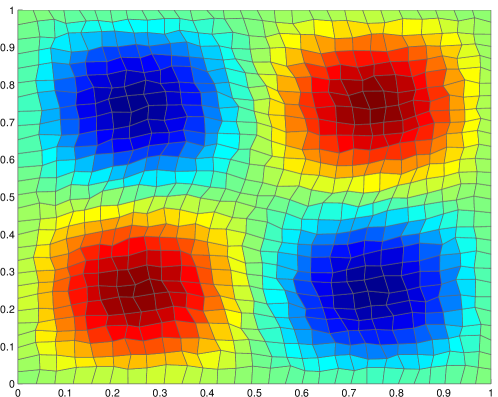
Figure 2. Example of a deformed grid, with refinement factor equal to 7 (The colors represents the displacement field in the $y$-direction computed using the MSPA method)

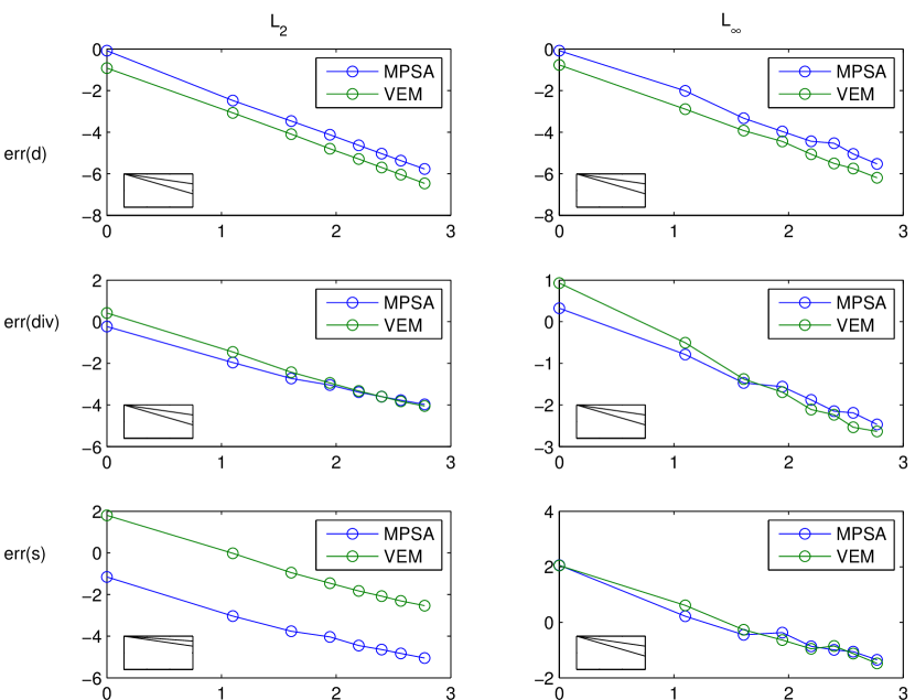
Figure 3. Convergence plot for a twisted Cartesian grid. The $L^{2}$-norm (left) and $L^{\infty}$-norm (right) of the error are plotted for the displacement (upper row), the divergence (middle row) and the stress (lower row). Logarithmic scales are used and the values on the x-axis give the logarithms of the refinement factor. In the small boxes, the slopes corresponding to a convergence factor for one and two are represented.

3.2. Case 3.2: Mixed cell types

We set up a case (Case 3.2) with a grid which mixes several difficulties. The grid is made up by, first, assembling regions with different cell types (triangles, quadrilaterals, hexahedral) and, then, twisting the grid. Many cells have unfavorable aspect-ratio. There are also hanging nodes. However, as it can be seen from Figures 4, 5 and 6, the methods manage to capture rather well the exact solution. Note that MPSA has problem to handle triangles where not all the angles are smaller than $90$ degrees. Nevertheless, the error that can be made on these cells does not spread to the whole domain.

We investigate further the case of large aspect ratio for hexahedral (Case 3.2) and triangular grid (Case 3.2). Both grids are obtained by stretching uniform grids in the $x$-direction with a given factor. In both cases, we use an aspect ratio of $7$. In Figure 7 and 8, we observe that the VEM method manages to handle the hexahedral case correctly while, for the grid made by triangles, it produces reliable values for the displacement field but oscillatory values for the divergence. As far as the MPSA method is concerned, we exceed the restrictions on the grid that the method requires and the method fails, see Figure 7. The case of the triangle grid is not plotted for the MPSA method.

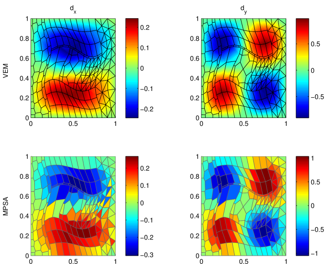
Figure 4. Displacement field $\bm{u}$ (Case 3.2) for the MPSA and VE methods.

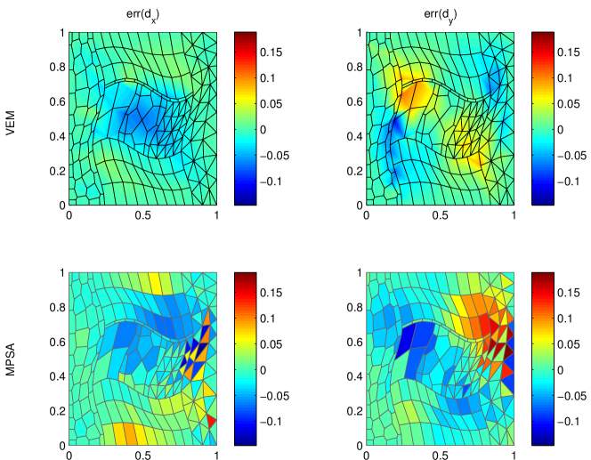
Figure 5. Error in the displacement field $\bm{u}$ for both methods (Case 3.2).

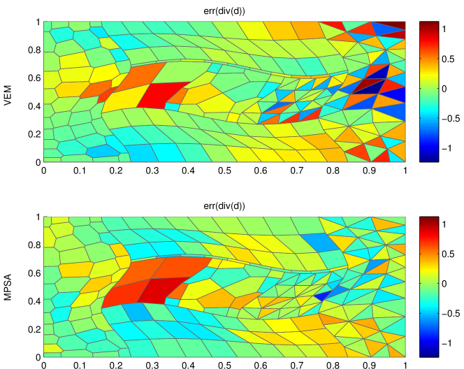
Figure 6. Error in the divergence field $\nabla\cdot\bm{u}$ for both methods (Case 3.2).

	$d_{x}$	$d_{y}$	$\nabla\cdot\bm{u}$
VEM
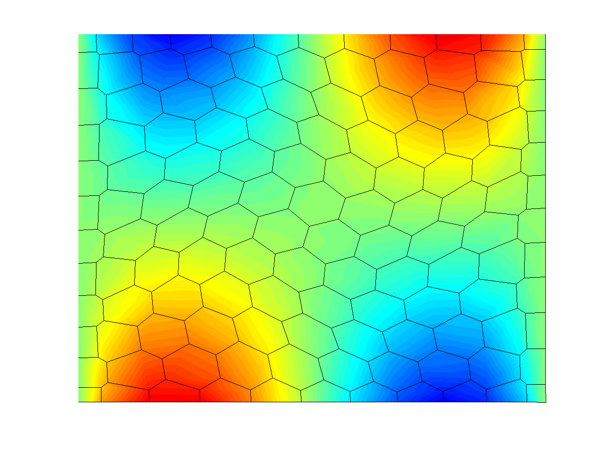
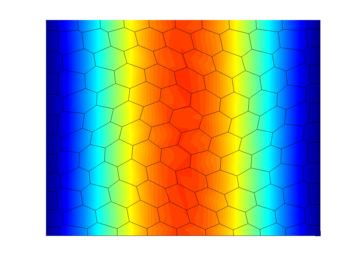
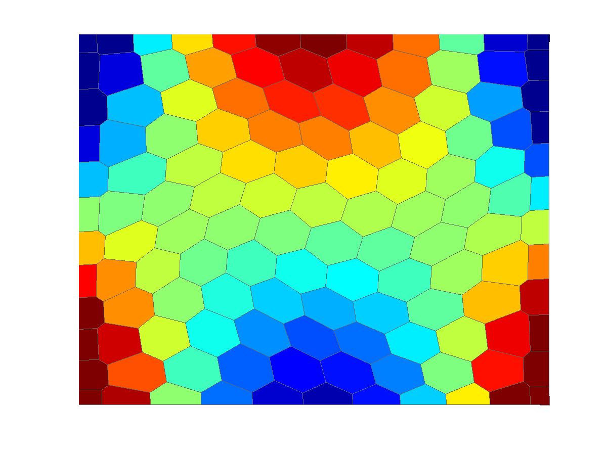
MPSA

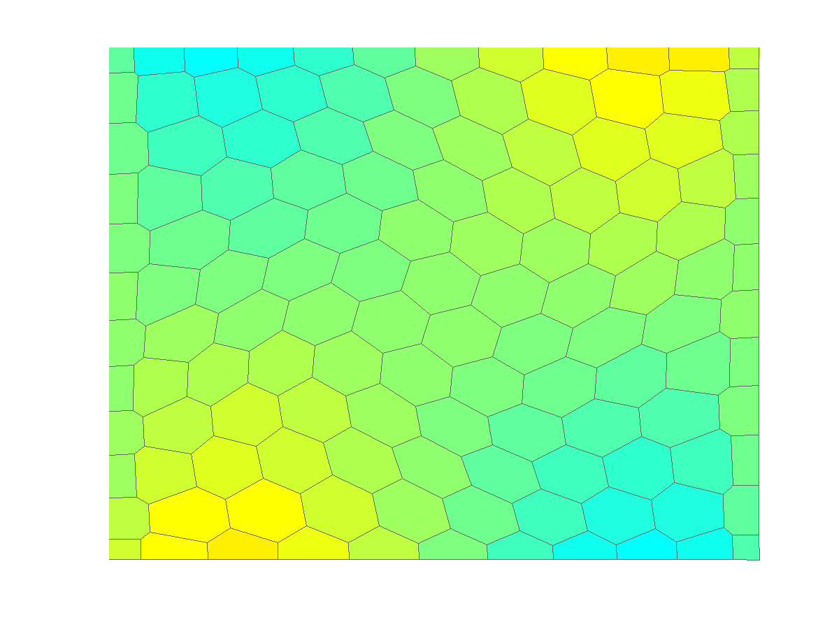
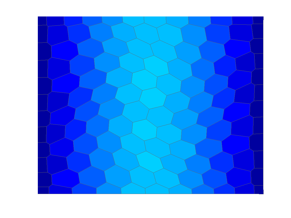
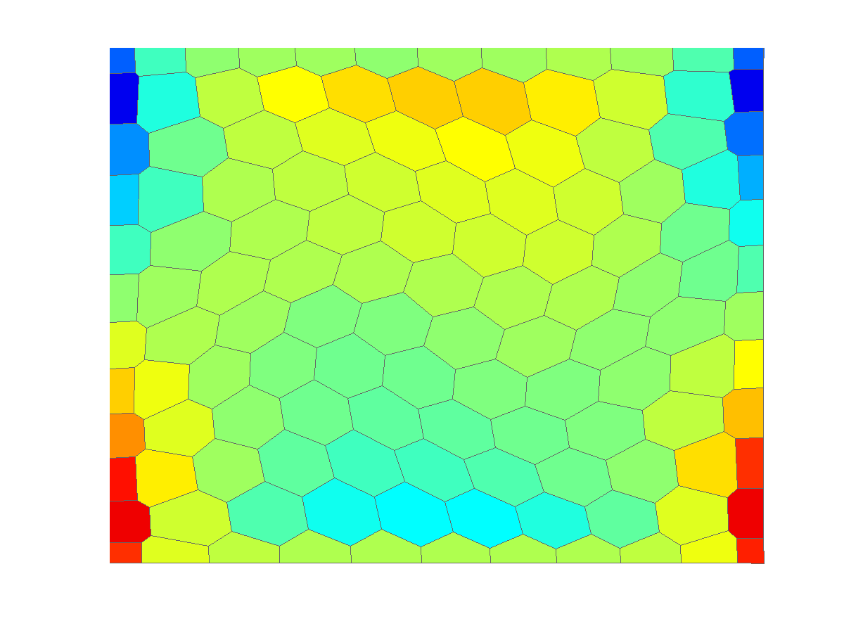
Figure 7. Aspect ratio $7$ using an hexahedral grids (Case 3.2). For the purpose of a better visualization, we plot the values of the displacement and divergence fields on a grid which is stretched back to a uniform grid (with aspect ratio $1$).

	$d_{x}$	$d_{y}$	$\nabla\cdot\bm{u}$
VEM

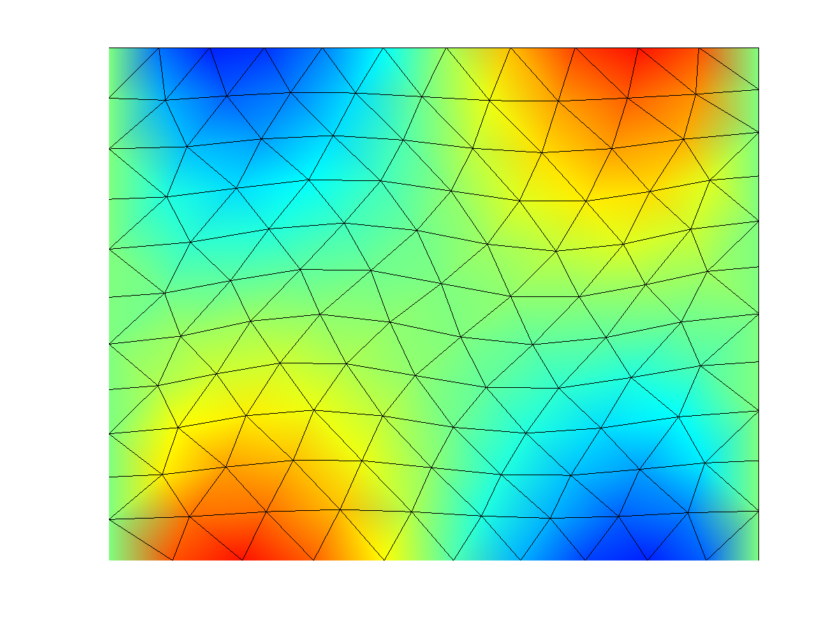
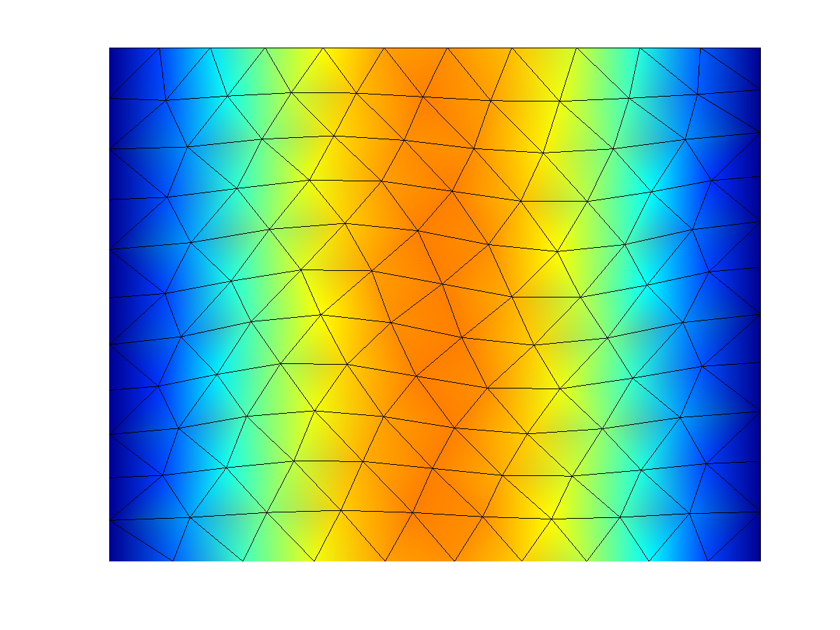
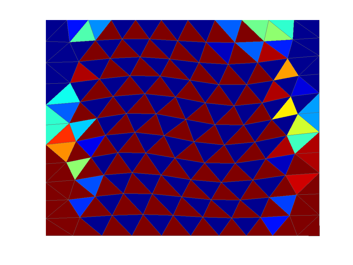
Figure 8. Aspect ratio $7$ using a triangular grid (Case 3.2). The same visualization procedure as in Figure 7 is used here.

3.3. Case 3.3: Stability for refinement in one direction

Grids of stratigraphic subsurface models are often designed with long and flat cell-blocks which reflect the layered structure of the rock. Such cell-blocks have deteriorated aspect ratio. We set up an example to test the robustness of the methods with respect to such deterioration of the grid. We use a Cartesian grid which is refined in the $y$ direction. Moreover, the grid is twisted to break symmetry effects which may improve artificially the results. In Figures 10 and 9, we plot the error. Of course, even if we increase the number of cells, we cannot expect any improvement of the solution in this case but we can see that the solutions are not significantly impaired by the refinement and the deterioration of the grid. The $L^{2}$-norms of the error for the stress are substantially different for the two methods, but we recall that these values are not directly comparable, see the comments at the beginning of Section 3.

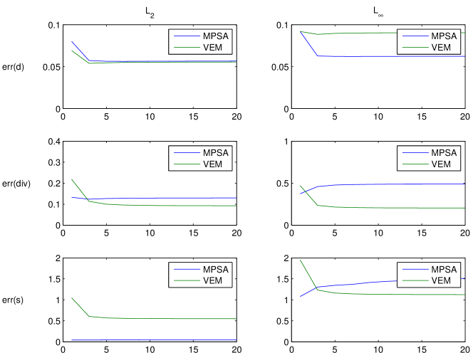
Figure 9. Plot of the errors when the grid is uniformly refined in the $y$-direction before being twisted (Case 3.3). We consider the The $L^{2}$ norm (left) and $L^{\infty}$-norm (right) of the errors for the displacement (upper row), the divergence (middle row) and the stress (lower row). The error remains under control for all methods even when the aspect ratio deteriorates. The $x$-axis indicates the refinement ratio in the $y$-direction.

Figure 10. Plot of the displacement in both the vertical and horizontal directions for Case 3.3. In this figure, the refinement ratio is 10.

3.4. Case 3.4: Stability with respect to decomposition of the grid in regions with different refinement

Grids in subsurface simulations are typically heterogeneous, mixing cells of different sizes and shapes. We consider two test cases where two regions of equal size but with different refinements are set side by side. For the first case (Case 3.4), the refinement in the region on the right-hand side is done in both $x$ and $y$ direction. For the second case (Case 3.4), it is done only in the $y$ direction. In both cases, we have a coarse domain on the left-hand side.

In Figure 11, we look at the error when the refinement on the right-hand side is increased in both directions. By refinement factor, we mean the number of sub-intervals that an edge of the initial grid is divided into to obtained the refined grid. We observe that the error for the VE method increases significantly for the divergence of the displacement and the stress in the $L^{\infty}$-norm. In the $L^{2}$-norm, the increase is much less severe, which indicates that error is essentially of local nature. In Figure 12, we plot the force at the interface between the two regions. For the VE method, the stress is defined inside the cells so that we obtain two curves at the interfaces, one for the coarse cells, the other for the fine cells. The force is computed at a cell interface by integrating the product of the stress in the cell with the normal of the interface. For the MPSA method, the force is defined on the edges and is therefore readily available at the interface. We observe that the stress for the VE method is strongly oscillating in the cells which belong to the refined region. For the horizontal component of the force, the oscillations take the form of peaks, while the force computed from the cells belonging to the coarse region is smooth and rather close to the analytical value which is zero due to the symmetry of the problem. For the $y$-component of the force, the analytical value is no longer constant. For the VE method, the value computed from the cells of the fine region still presents oscillation but, in addition, the value computed from the coarse region presents strong variations, approximating the smooth analytical values by a staircase function. Such behavior may be problematic if the solver is coupled with a fracture model, typically non-linear, based on local value of the stress field. In comparison, the MPSA method yields much smoother approximations. In Figure 13, we plot the error in displacement at the interfaces. From this figure, it is clear that the local error concentrates at the hanging nodes, see also Figure 14.

Let us now consider the case where the refinement is done only in the $y$-direction (Case 3.4). The discretization at the interface is the same as in the previous case but the cells at the right-hand side get a relatively larger area and a larger aspect ratio. In Figure 15, we observe that the error in the $L^{\infty}$-norm no longer grows for the VE method. The strong oscillations in the $x$-component of the force are smaller compared to the previous case, as we can observe by comparing Figures 12 and 17. We can see in Figure 18 that most of the local error occurs at the non hanging nodes. For the MPSA method, oscillations that were not present in Case 3.4 now appear in case 3.4. Moreover, we can see in Figure 16 that the error spreads to the layer of coarse cell lying at the interface, especially for the error in the divergence term. The calculation of the divergence term in the MPSA method is based on the continuity points at the boundary, which is calculated from solving a local problem.

Finally, we setup a case where the two regions have the same coarse mesh but we add extra nodes at the interface (Case 3.4). In this way, we remove the difference in volumetric refinement between the two regions and isolate the effect of edge refinements. In Figure 19, we plot the error displacement for the VE method at the interface and observe that the nodes which belong to both a long edge and a short edge behave differently than the nodes that belong to two small edges (in this case, the hanging nodes). This observation complies with the results observed earlier and presented in Figure 13 and Figure 18, which shows that the VE method spreads the error unevenly between these two types of nodes. Second, it shows that it is related to edge refinement. In the VE method, the basis elements are not computed, only the degrees of freedom are used for the assembly and linear approximations remain exact but, in the case of elements with many nodes, the basis elements will be highly non-linear. We illustrate this in Figure 20 where we compute some of the virtual basis elements constructed using harmonic lifting as in [7], see also [18]. We consider the same type of cells as the ones which lie at the interface in Case 3.4, reducing the refinement to ten nodes in order to make the pictures easier to read. For simplicity, this illustration has been created using the Laplace operator and not the linear elasticity operator. We can sort the virtual basis in three categories:: Basis with two large edges (type I), basis with a large and a small edge (type II), basis with two small edges (type II). The virtual basis elements have very sharp gradients in small regions and are almost flat elsewhere so that most of their energy is concentrated in high frequencies. In this case, the projection operator $\mathcal{P}$ over linear function, see section 2.1, does not provide a good approximation and most of the contribution for this basis element will be handled by the regularization term, $s_{K}$, which is only a poor substitute for $a_{K}$. We have computed the residual part for the three basis,

$$\frac{a_{K}(\phi-\mathcal{P}\phi,\phi-\mathcal{P}\phi)}{a_{K}(\phi,\phi)}=\begin{cases}0.49&\text{ if $\phi$ is of type I,}\\ 0.90&\text{ if $\phi$ is of type II,}\\ 0.99&\text{ if $\phi$ is of type III.}\end{cases}$$

Since in this case the length of the large and small edges are $L=1$ and $l=0.1$, respectively, these computations confirm the following orders of magnitude,

$$\frac{a_{K}(\mathcal{P}\phi,\mathcal{P}\phi)}{a_{K}(\phi,\phi)}\approx\begin{cases}1&\text{ if $\phi$ is of type I,}\\ l/L&\text{ if $\phi$ is of type II,}\\ (l/L)^{2}&\text{ if $\phi$ is of type III,}\end{cases}$$

which can be obtained by roughly estimating the area of the support of the gradient of the basis function. In Figure 13, we observe that, at the interface region, the displacement values obtained at nodes that are connected to a large edge (which we denote type A) have different errors that the other nodes (which we denote type B), see a zoom on this region in Figure 21.

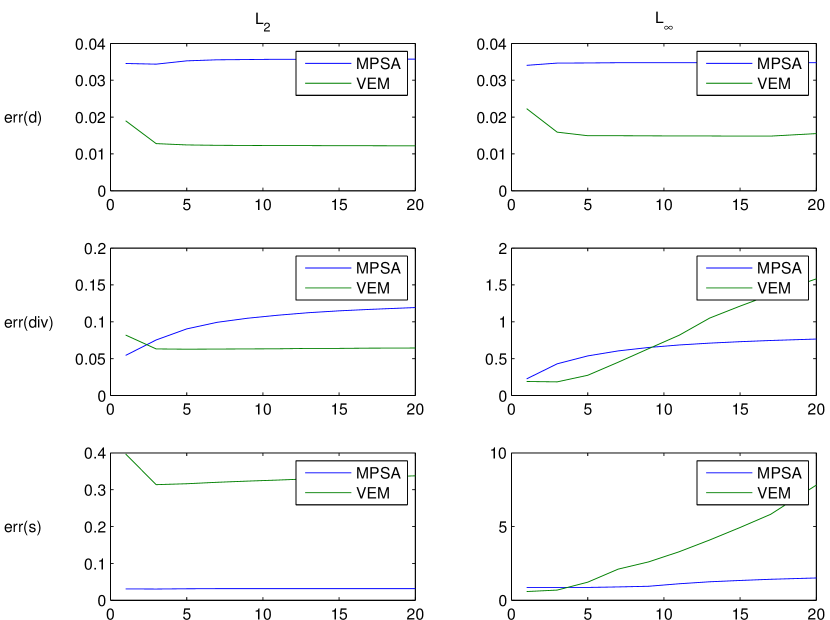
Figure 11. The region at the right-hand side is refined equally in both the $x$ and $y$ direction (Case 3.4). The $L^{2}$-norm (left) and $L^{\infty}$-norm (right) of the error are plotted for the displacement (upper row), the stress (middle row) and the divergence (lower row). The $x$-axis indicates the refinement factor in the right-hand side region.

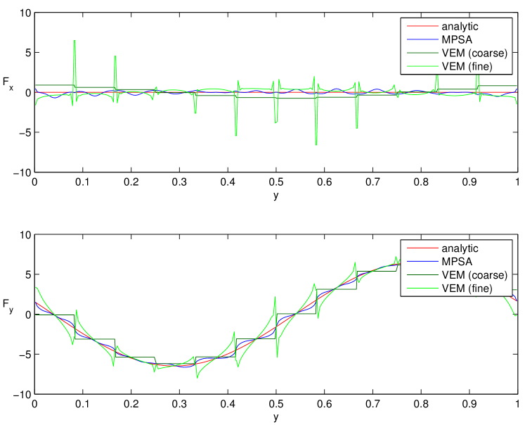
Figure 12. Plot of the forces at the interface between the two regions for Case 3.4. For the MPSA, the stress is computed on the faces so that the values of the stress at the interface are directly available. For the VE method, the stress is computed in the cells so that two values, one from the coarse and the other from the fine region, can be used to define the value of the stress at the interface.

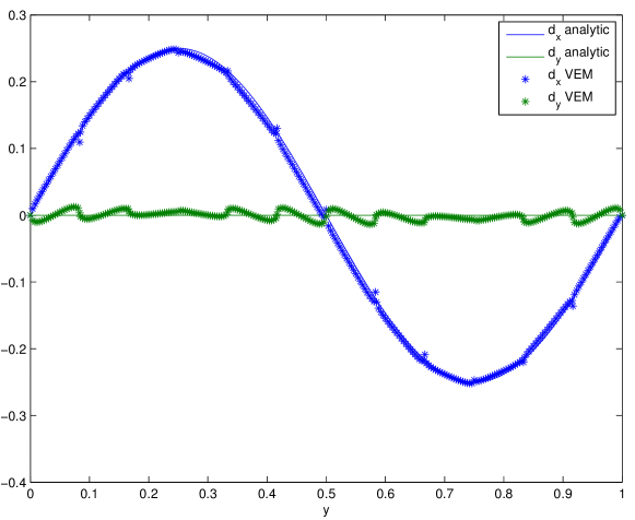
Figure 13. Plot of the error in displacement at the interface, only for the VE method (Case 3.4)

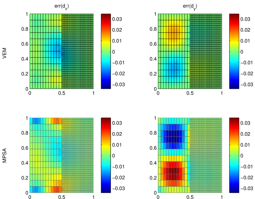
Figure 14. Plot of the displacement in both the vertical and horizontal directions (Case 3.4)

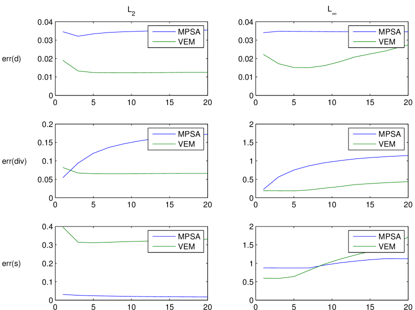
Figure 15. The region at the right-hand side is refined only in the $y$ direction (Case 3.4). The $L^{2}$-norm (left) and $L^{\infty}$-norm (right) of the error are plotted for the displacement (upper row), the stress (middle row) and the divergence (lower row). The $x$-axis indicates the refinement factor in the right-hand side region.

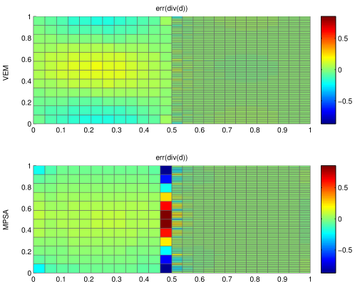
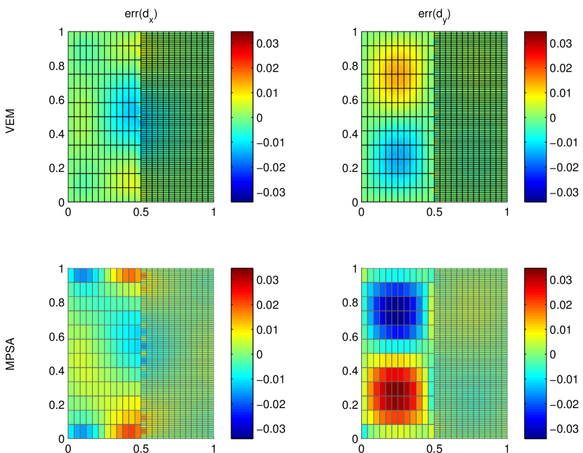
Figure 16. Plot of the error in the divergence (two upper plots), the horizontal displacement (two lower left plots) and the vertical displacement (two lower right plots) for Case 3.4. The vertical refinement ratio in the region on the right-hand side is equal to 20.

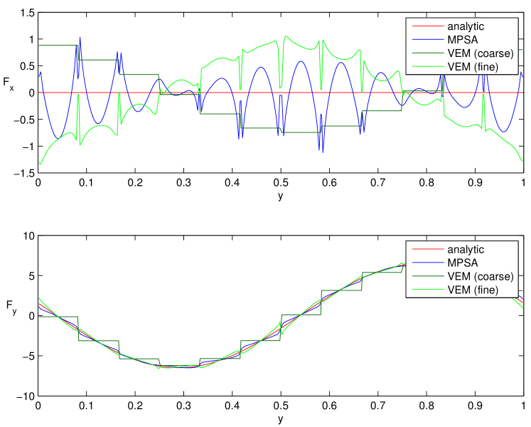
Figure 17. Plot of the forces at the interface, for Case 3.4. The values are obtained in the same way as in the plot of Figure 12.

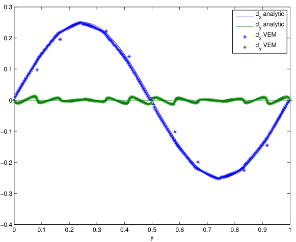
Figure 18. Plot of the error in displacement at the interface, only for the VE method (Case 3.4)

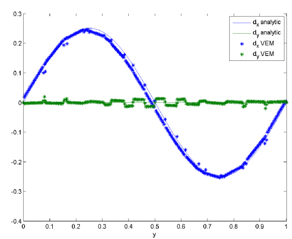
Figure 19. Plot of the error in displacement at the interface, only for the VE method in the case where there is no layer but 20 extra nodes on each face at the interface (Case 3.4).

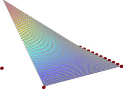
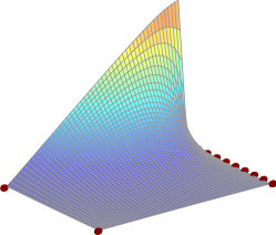
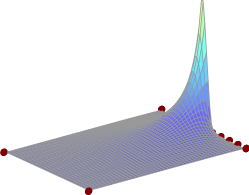
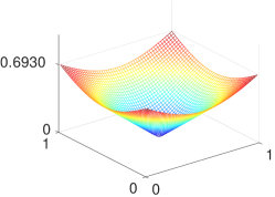
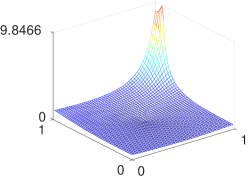
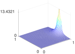
Figure 20. Illustration for Case 3.4 using the Laplace operator. First row: Plot a three virtual basis elements for a square cell with 10 edges on one side. The red dots indicates the position of the nodes. We can sort the virtual basis in three types: Basis with two large edges (left), basis with a large and a small edge (middle), basis with two small edges (right). Second row: Plot of the norm of the residual of the projection, that is $\left|\nabla(\phi-\mathcal{P}\phi)\right|^{2}$, for the basis function represented above.

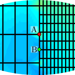
Figure 21. Zoom of the interface region showing the error in horizontal displacement for the VE method in case 3.4, see Figure 14. The error is different at nodes with a large edge (type A) and nodes which connect to two small edges (type B).

3.5. Case 3.5: Layer between two domains

In subsurface flow, an important part of the flow is concentrated in the fractures of the rock. We set up test cases that reproduce the geometry of a fracture by introducing a thin layer in an otherwise uniform Cartesian grid. If this layer were a fracture or a damaged zone, then it would have very different mechanical properties than the rest of the matrix, but, in our test case, the layer is assigned the same properties as the rest of the domain so that the analytical solution given by (34). In this way, we isolate the errors of the two numerical methods which are induced by a typical geometrical discrete representation of a fracture, without including the mechanical effects of the fracture itself. First, we consider a test case (Case 3.5), where the layer is discretized with the same level of refinement in the $y$ direction as the rest of the matrix. In Figure 22, we let the width of the layer get thinner and thinner. We observe that the error does not grow, indicating the robustness of both methods with respect to the thickness of the layer. Figure 23 gives the error in displacement and divergence of displacement. We observe that the error in displacement is more localized for the VE method and more spread for the MPSA method, which is consistent with the results of Figure 22 when comparing the $L^{\infty}$ norm and $L^{2}$-norms. In Figure 24, we present a plot of the forces at the interface between the layer and the region with coarse cells. We choose the left interface of the layer but the results on the other interface have the same characteristics. We observe that the MPSA method gives slightly but not significantly better approximation of the force.

In applications, the discretization level of the fracture layer may typically not match the one of the matrix. We investigate this situation by setting up a test case where the refinement in the layer is increased (Case 3.5). We also consider the same case but we twist the grid (Case 3.5) to break eventual symmetry effects. In Figure 25, we can observe the $L^{\infty}$-norm of the error for the stress grows significantly for the VE methods. The error in divergence remains zero in the Cartesian case (Case 3.5) but, by looking at the twisted case (Case 3.5), we conclude that this is only due to a symmetry effect. The error in displacement for this test case is plotted in Figure 26. In Figure 27 where a plot of the force is given at the interface, we observe that same oscillations for the VE method as previously in the case of two adjacent regions with different discretization levels (namely Case 3.4). Also in this case, the MPSA method gives a smoother approximation closer to the analytical solution. In Figure 28, we present a plot of the divergence along the interface together with a zoom on the region around of the error in divergence. Note that for the MPSA method, we use the finite volume definition of the divergence, that is, the value of the divergence in the cell is equal the sum of the normal component for each face. Again, we observe how the error in the VE method remains highly localized and concentrates inside the layer while the error for the MPSA methods spreads more to the coarse cell.

Figure 22. The width of the layer is decreased and no vertical refinement in the layer is used (Case 3.5). The $L^{2}$-norm (left) and $L^{\infty}$-norm (right) of the error are plotted for the displacement (upper row), the stress (middle row) and the divergence (lower row). The $x$-axis indicates the reduction factor for the width of the layer.

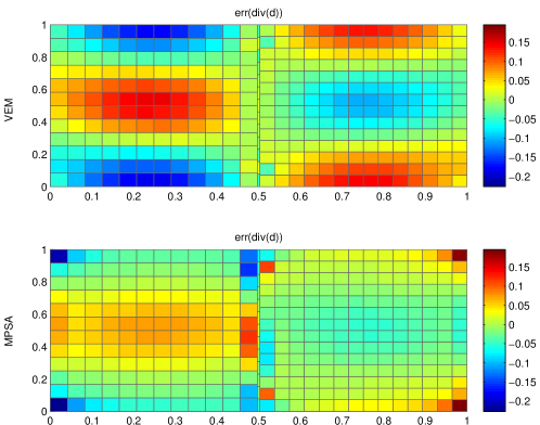
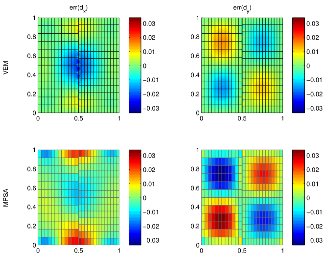
Figure 23. Error in the divergence (two upper figures) and the displacement in both $x$ and $y$ directions (Case 3.5). The width of the layer is 20 times smaller than the adjacent cells.

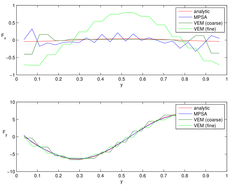
Figure 24. Plot of the forces at the interface, for Case 3.5. The values are obtained in the same way as in the plot of Figure 12.

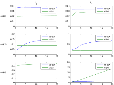
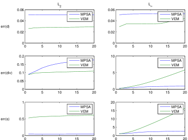
Case 3.5	Case 3.5

Figure 25. The width of the layer is decreased but the aspect ratio of the cells in the layer is preserved. The $L^{2}$-norm (left columns) and $L^{\infty}$-norm (right columns) of the error are plotted for the displacement (upper row), the stress (middle row) and the divergence (lower row). On the left, we have the Cartesian case (Case 3.5) and the twisted case on the right (Case 3.5). In all plots, the $x$-axis indicates the value of the reduction factor of the layer width.

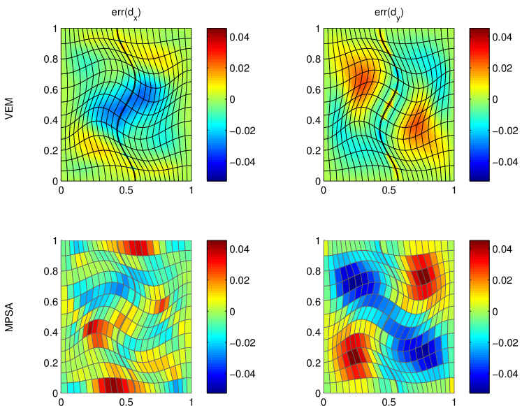
Figure 26. Plot of the error of the displacement in $x$ and $y$ directions (Case 3.5).

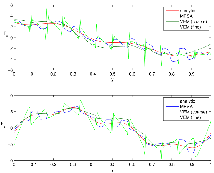
Figure 27. Plot of the forces at the interface, for Case 3.5. The values are obtained in the same way as in the plot of Figure 12.

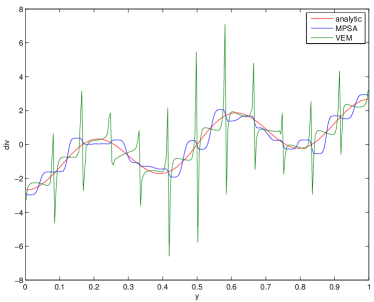
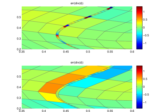
Figure 28. Plot of the divergence at the interface of the layer for Case 3.5 (top). We observe large oscillations for the VE method (middle) inside the layer but they remain confined in the layer. Comparatively, the oscillations are weaker for MPSA (bottom) but the error spreads more to the neighboring cells.

3.6. Case 3.6: Stability near incompressibility

In the following experiments, we set up cases to test the method with respect to the near incompressibility limit. The boundary conditions are zero displacement on the left and right side and free displacement on the top and bottom side. The external force is a constant volumetric vertical force, like for example a gravitational force. We present test results for three grid types which highlights the main features. We consider grids made of hexahedrons (Case 3.6), triangles (Case 3.6) and quadrilaterals (Case 3.6). To generate each grid, we start with a uniform tessellation. Then, the grid is twisted in order to remove any side-effects that may arise from symmetry. In the case of hexahedrons (Case 3.6), we observe numerical locking for VEM and MPSA while VEM-relax, VEM-relax-extra and MPSA-relax-extra give a good approximation of the solution. The numerical locking for VEM can be observed directly in the displacement field where we can see that the medium appears to be much stiffer than it actually is, hence the name of locking. The numerical locking for MPSA is more visible in the divergence field as artificial oscillations. Note that we could have chosen the parameter $\nu$ closer to 0.5 where the effects of numerical locking lead to a completely different solution, but we prefered to show examples where we can both recognize the solution and see the beginning of the perturbations caused by locking. In a grid made of hexahedrons, the ratio between the number of nodes and number of cells is typically large. As discussed in Section 2.3.2, such configuration is favorable for the VE method and disadvantageous for the MPSA method. Each node does not belong to more than three edges and the stability condition given in [19] is fulfilled. Therefore, the solution given by VEM-relax is free from locking effect and VEM-relax-extra does not bring any improvement. Let us now consider the grid made of triangles (Case 3.6). In this case, we observe that numerical locking affects the VEM and VEM-relax methods but MPSA, MPSA-relax-extra and VEM-relax-extra remain unaffected. In the case of a triangular grid the ratio between the number of nodes and number of cells is typically small and equal to the inverse of the same ratio for a hexahedral grid. Then, we explained in section 2.3.2 why this situation favors MPSA and penalizes VEM. This analysis is consolidated by the numerical results. We observe that the relaxation of the VE method is not enough to get rid of the numerical locking and extra degrees of freedom are required. We also note that the solution obtained from MPSA-relax-extra contains slightly more oscillations and is not as good as the one obtained by standard MPSA. This result highlights the relaxation effect of the method, which means that, if numerical locking is not an issue, the standard MPSA is expected to give less error than MPSA-relax-extra. In the setting of VEM, it corresponds to the fact that, when there is no locking, VEM has in general a smaller error constant than VEM-relax, as the latter considers a less accurate approximation of the divergence, see (23) compared to (22). Finally, we consider a grid made of quadrilaterals (Case 3.6). In this case the ratio between the number of nodes and number of cells is close to one, so that neither the VEM or MPSA method is a priori favored. We observe that the VEM and VEM-relax methods suffer from locking. In comparison, the MPSA handles remarkably well this case and does not present any sign of locking. As predicted by the theory, VEM-relax-extra is free from locking.

	$d_{x}$	$d_{y}$	$\nabla\cdot\bm{u}$
VEM
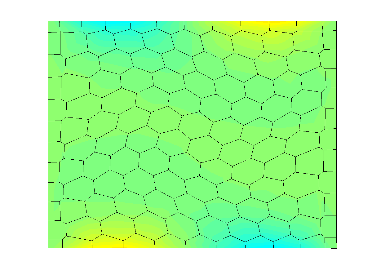
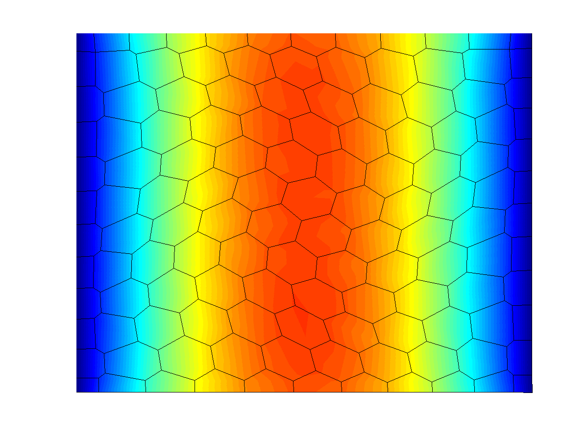
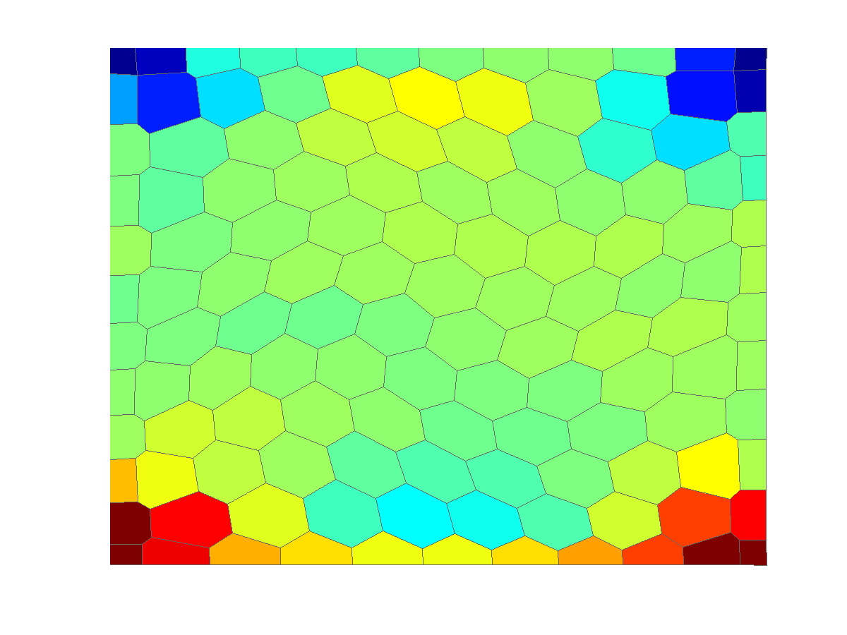
MPSA
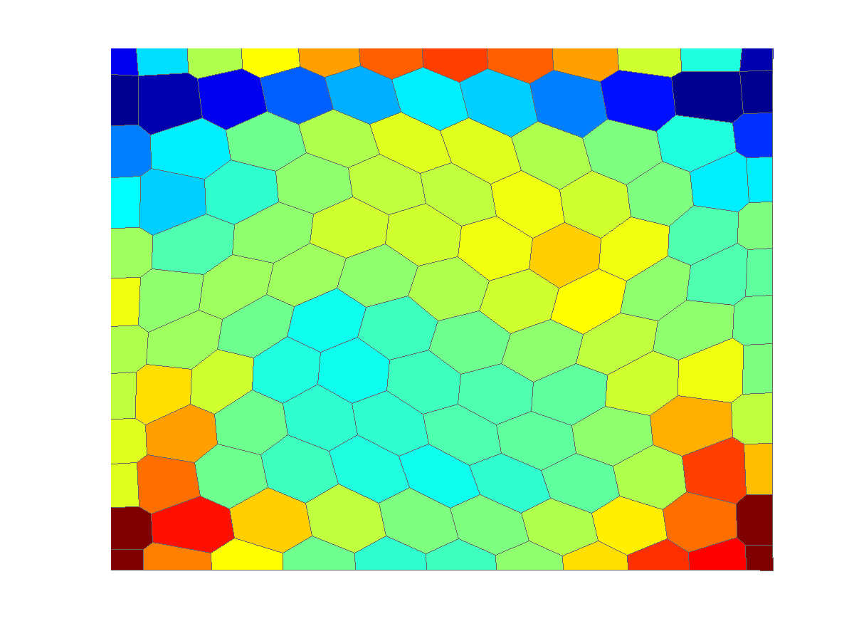
VEM relax
VEM relax extra
MPSA relax extra

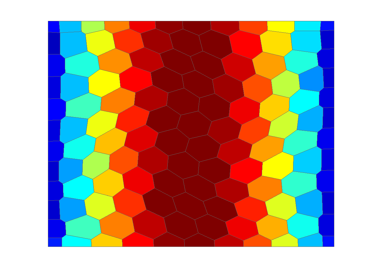
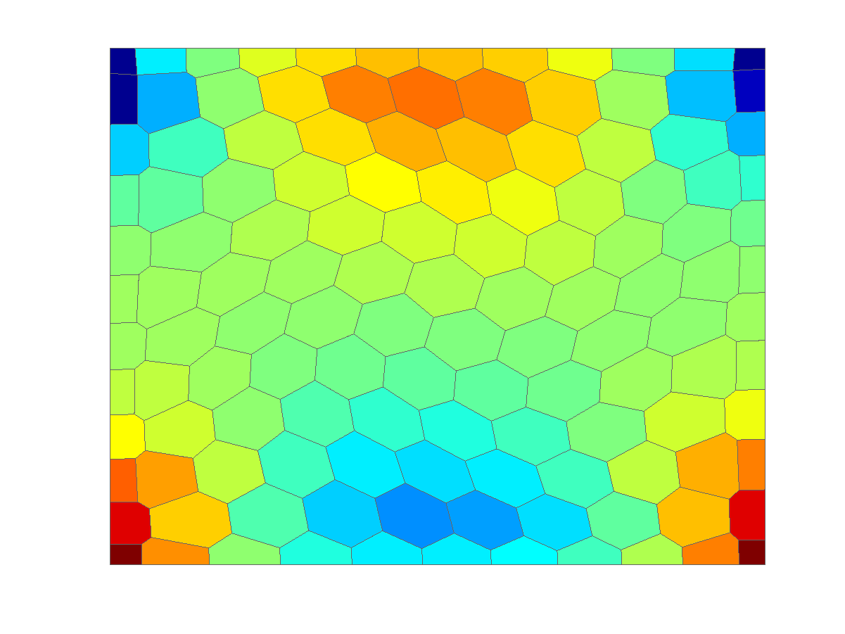
Figure 29. Hexahedral grid and $\nu=0.495$ (Case 3.6). MPSA and VEM suffers from numerical locking. VEM-relax and VEM-relax-extra are free from numerical locking.

	$d_{x}$	$d_{y}$	$\nabla\cdot\bm{u}$
VEM
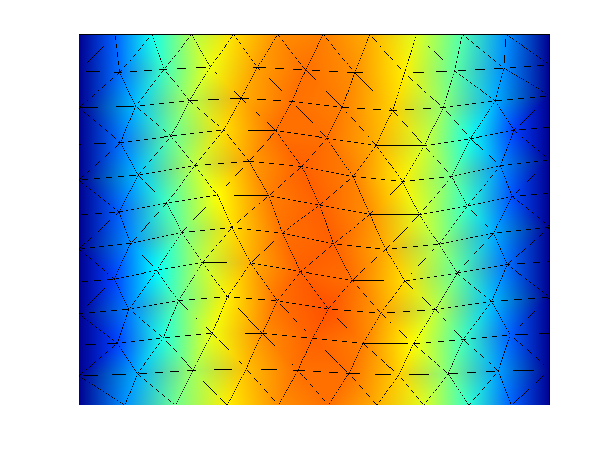
MPSA
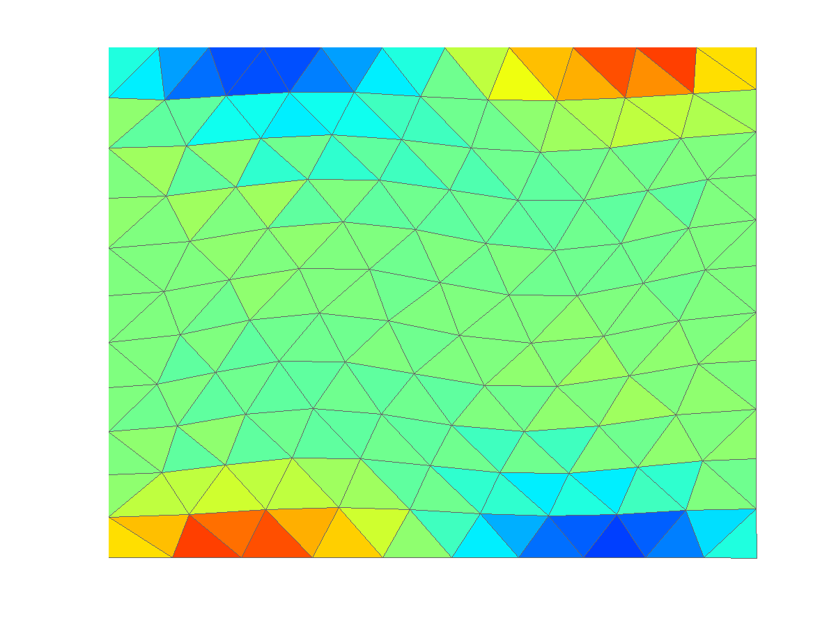
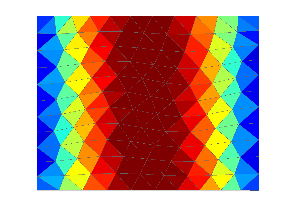
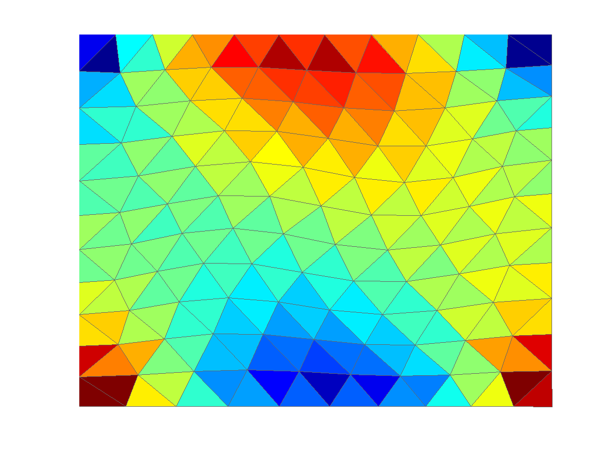
VEM relax
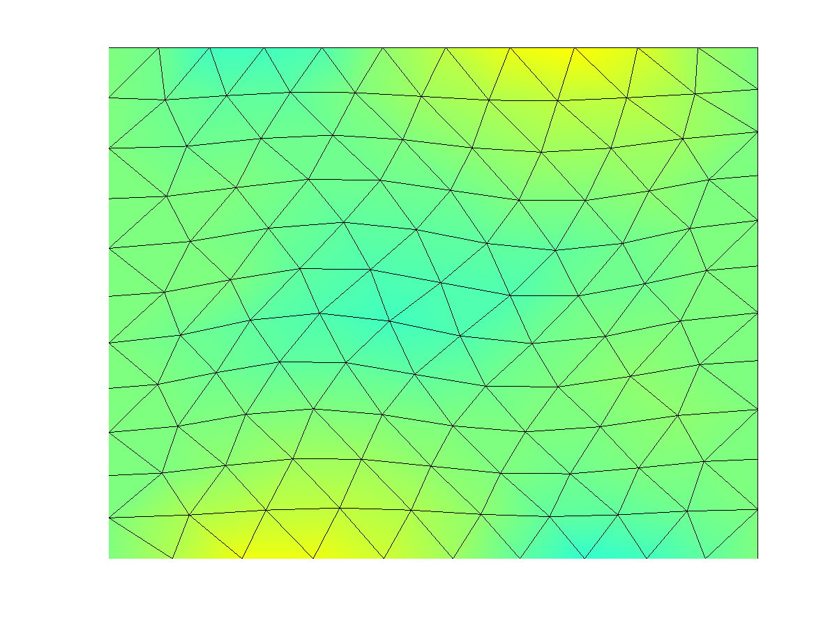
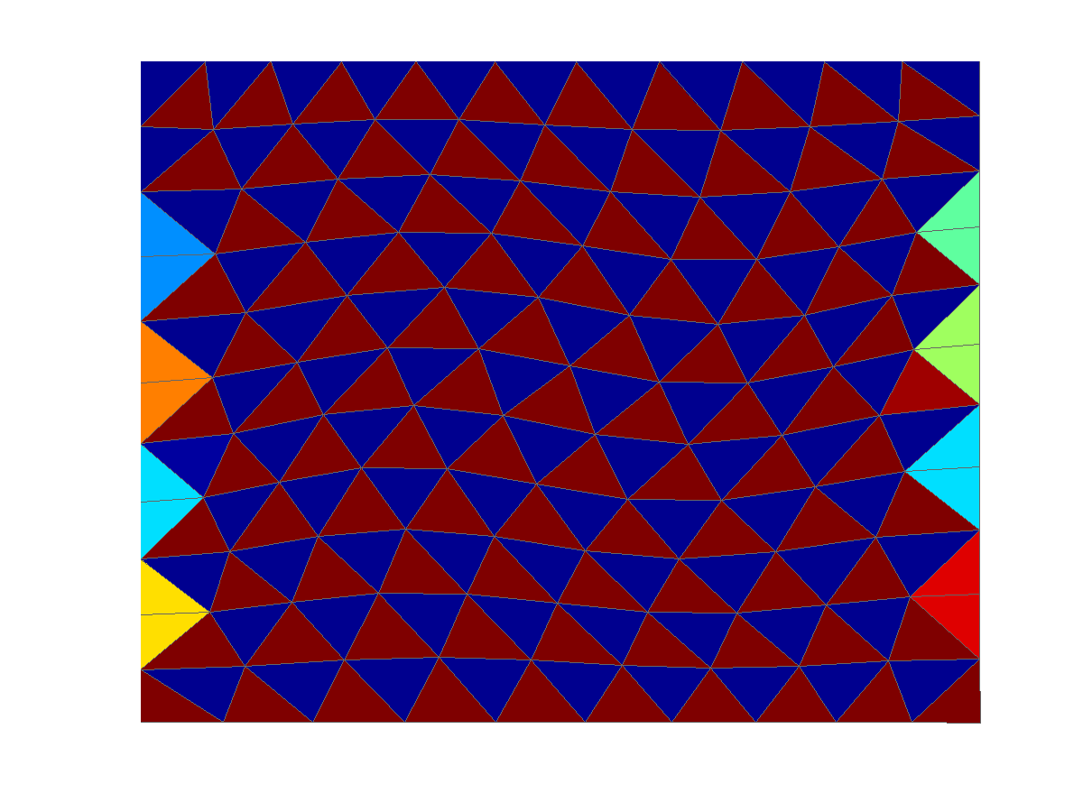
VEM relax extra
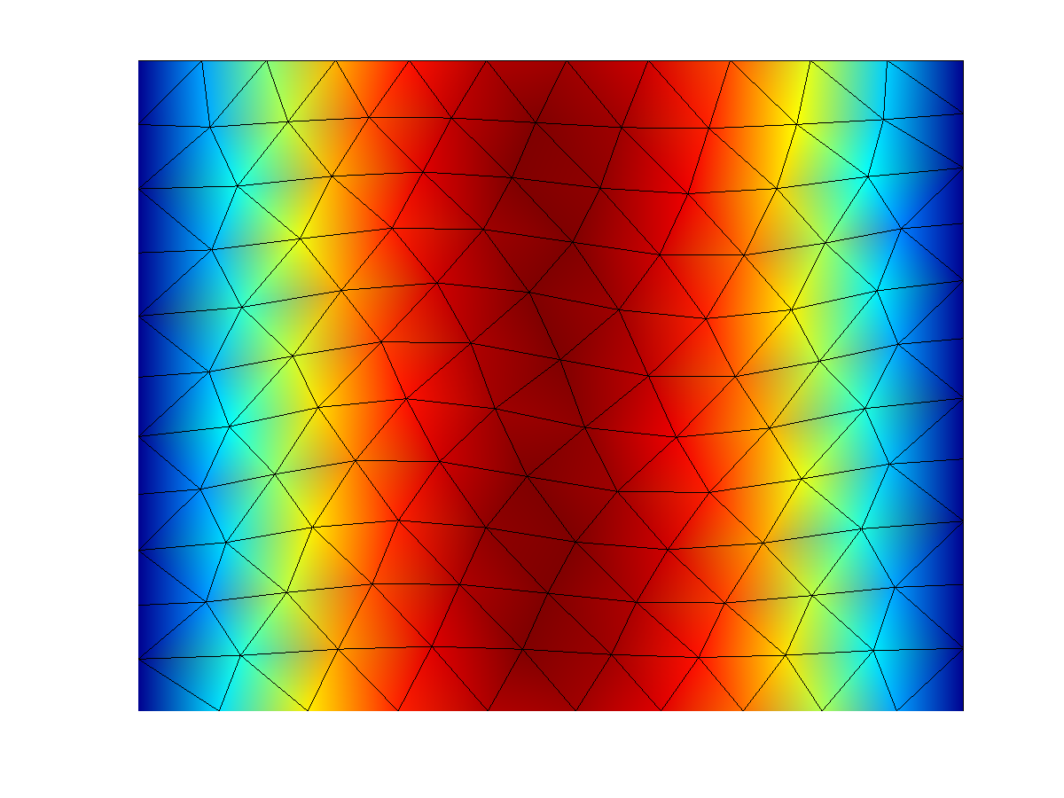
MPSA relax extra

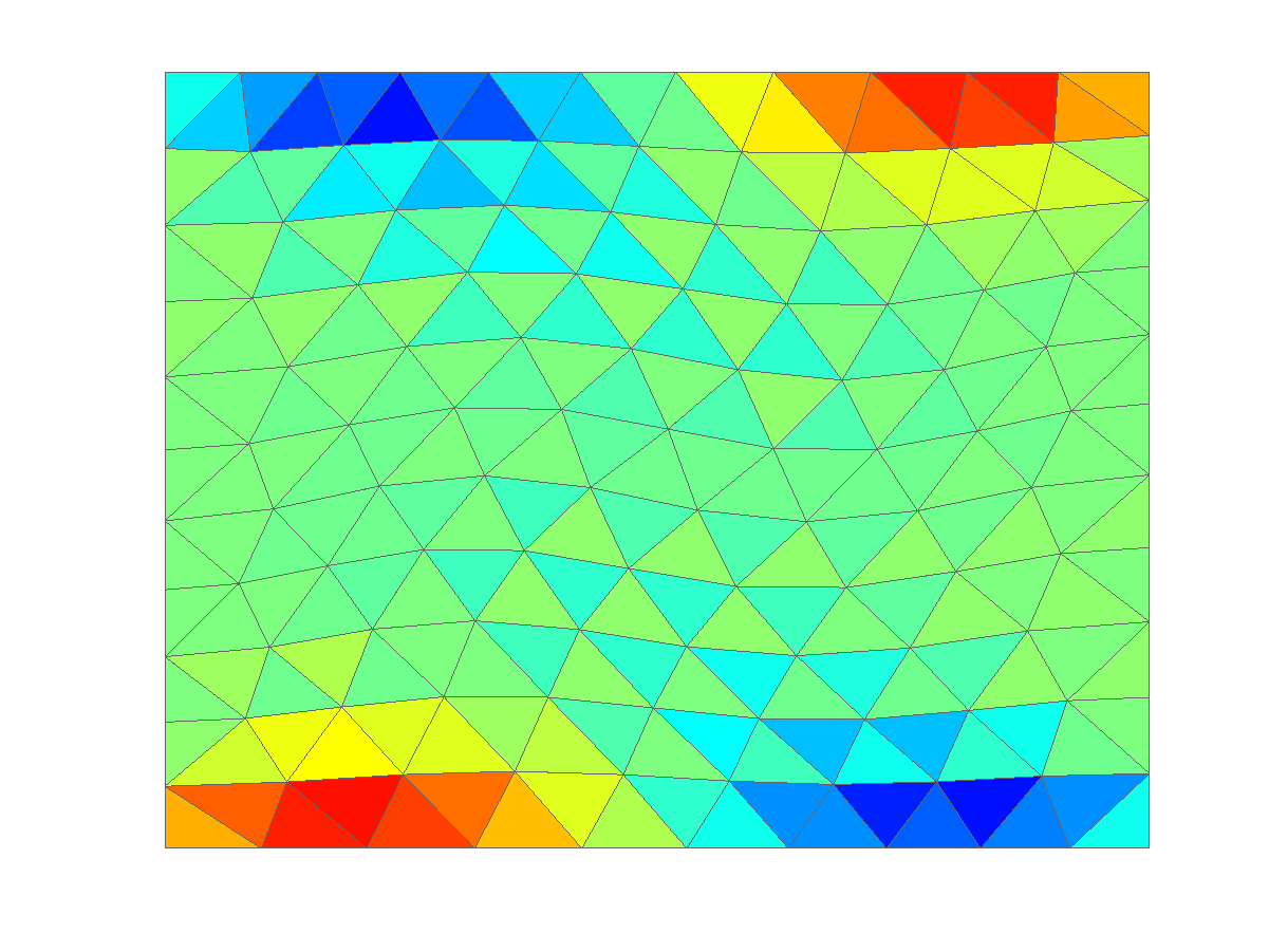
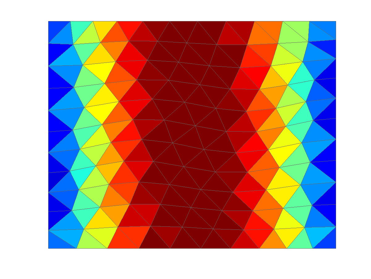
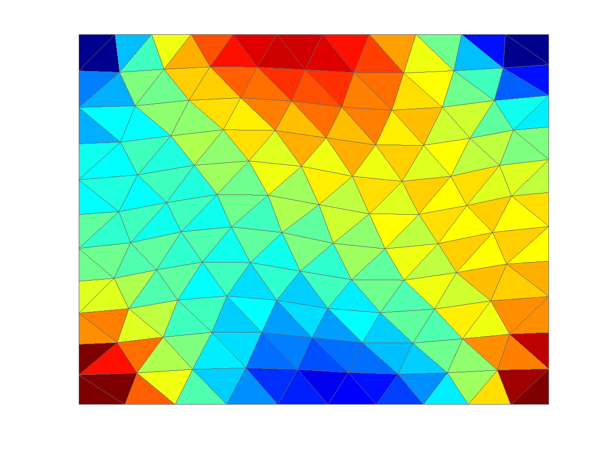
Figure 30. Triangular grid and $\nu=0.495$ (Case 3.6). VEM and VEM-relax suffers from numerical locking. MPSA and VEM-relax-extra are free from numerical locking.

	$d_{x}$	$d_{y}$	$\nabla\cdot\bm{u}$
VEM
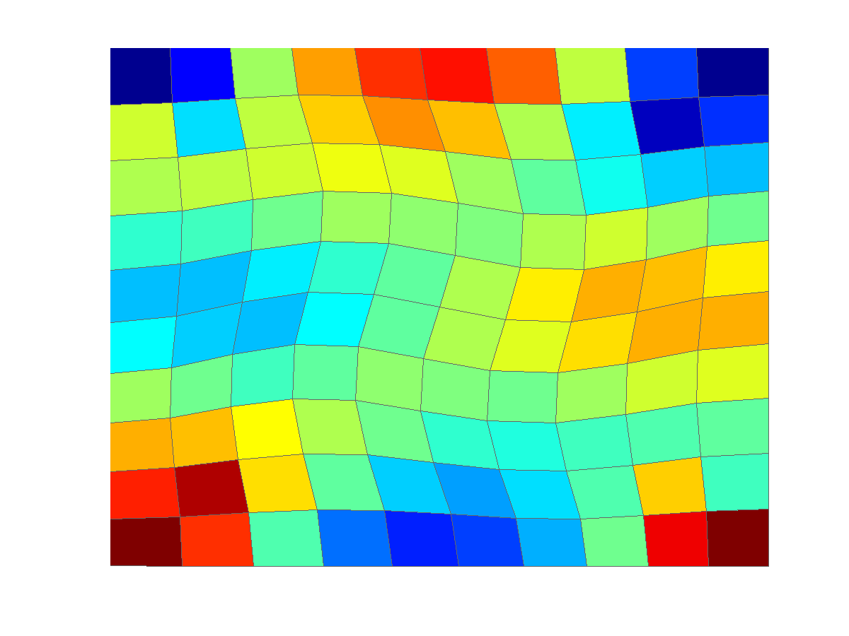
MPSA
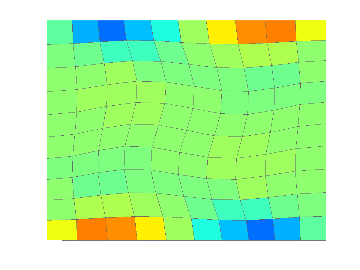
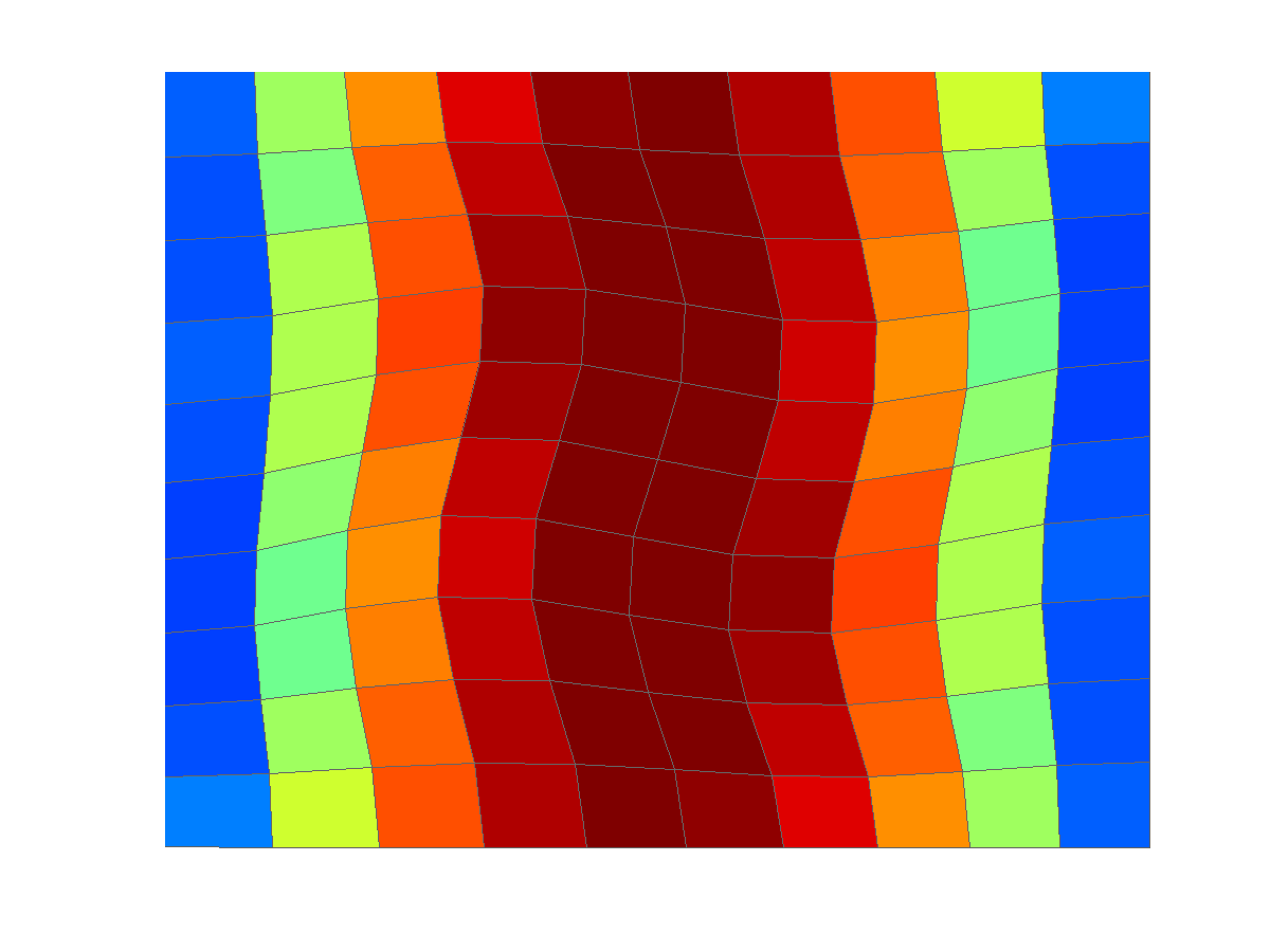
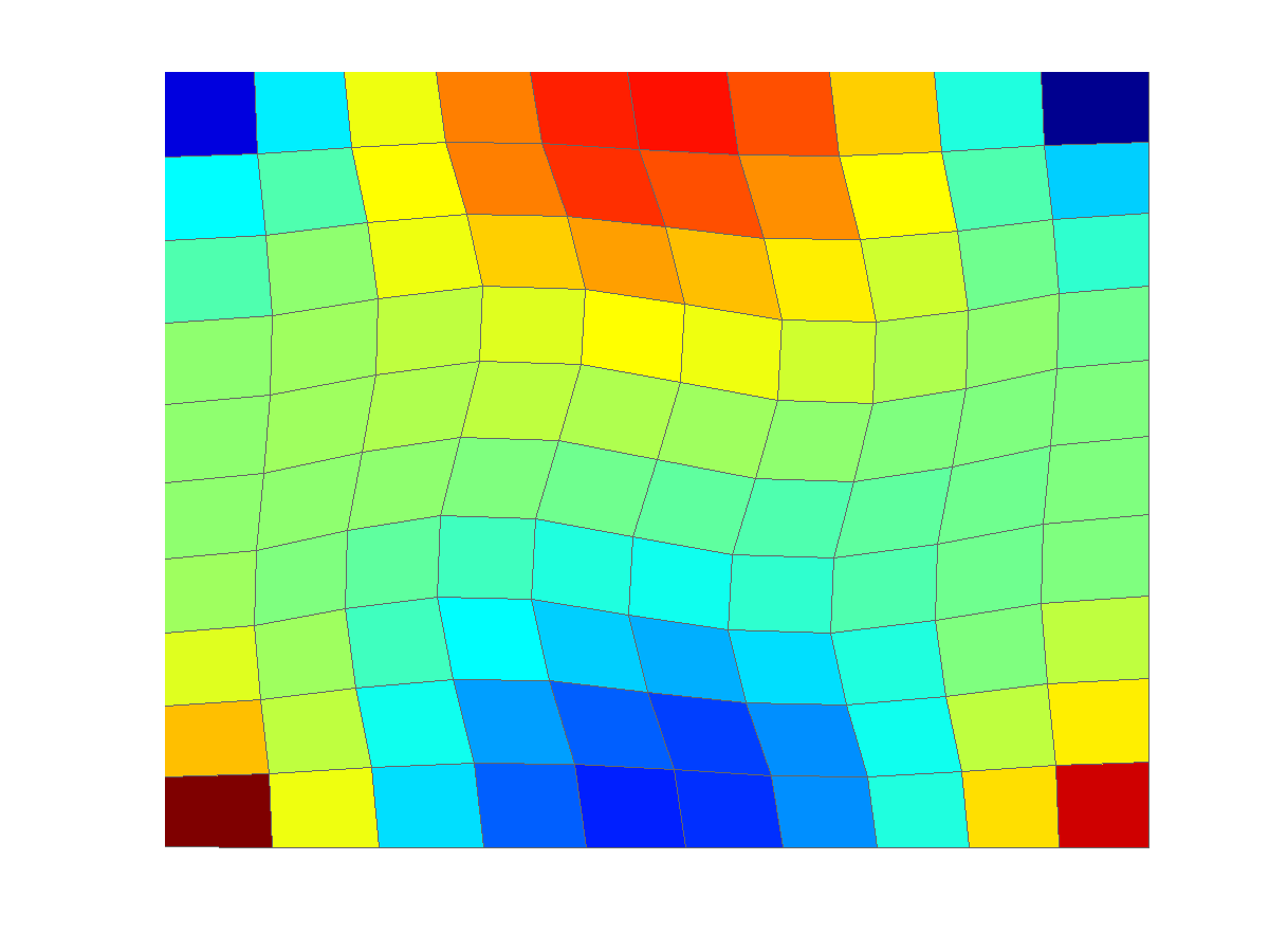
VEM relax
VEM relax extra
MPSA relax extra

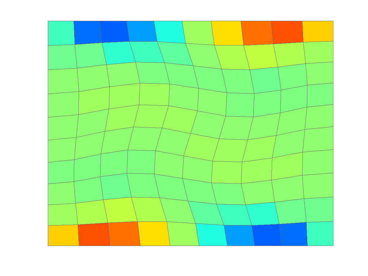
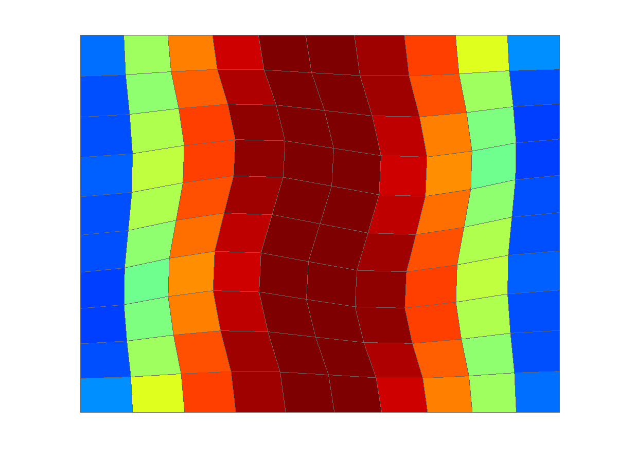
Figure 31. Quadrilateral grid and $\nu=0.495$ (Case 3.6). VEM and VEM suffers from numerical locking. MPSA does not present any sign of locking. VEM relax extra is free from locking, as predicted by the theory

Table 1. Summary of the numerical tests

Case 3.1 :	Twisted grid
Case 3.2 :	Mixed grid with challenging features
Case 3.2 :	Large aspect ratio with hexahedral grid
Case 3.2 :	Large aspect ratio with triangular grid
Case 3.3 :	Cartesian grid, with uniform refinement in the vertical direction
Case 3.4 :	Two regions, uniform refinement (both in $x$ and $y$) in one region
Case 3.4 :	Two regions, refinement only in the $y$ direction in one region
Case 3.4 :	Two regions with the same Cartesian discretization, but with 20 extra nodes in each face at the interface
Case 3.5 :	Vertical thin layer, no refinement inside the layer
Case 3.5 :	Vertical thin layer with refinement inside the layer, Cartesian grid
Case 3.5 :	Vertical thin layer with refinement inside the layer, twisted grid
Case 3.6 :	$\nu=0.495$ with hexahedral grid
Case 3.6 :	$\nu=0.495$ with triangular grid
Case 3.6 :	$\nu=0.495$ with quadrilateral grid

4. Conclusion

In this paper, we have tested the behaviors of the VE and MPSA methods for linear elasticity with respect to grid features and parameter values that are typical to subsurface models. We can conclude that both methods are capable to handle in a satisfactory manner the polyhedral grid structures that are standard in such models. A priori, both methods have relative advantages. The MPSA method is attractive from the physical point of view, due to the explicit treatment of the force continuity at the cell interfaces. The MPSA offers a natural stable coupling with poro-elasticity, see [14]. From the implementation point of view, the MPSA method is cell-centered and therefore shares the same grid structure as the MPFA method, which is also often the preferred convergent method for multi-phase flow. The VE method has the advantage of robustness. Obtained from a variational principle, it is always symmetric definite positive. For simplexes, the method reduces to the finite element method so that the large collection of techniques developed for finite elements, such as preconditioning, super-convergence techniques or patch recovery can be relatively easily applied to VEM. When we use the approach presented in [7] as we do in this paper, the projection operators are given explicitly and do not require extra local computations as they usually do in a VE method, so that the local assembly has finally the same structure as in the traditional finite element method. If one is interested in generating the deformed grid obtained from a computed displacement field, another advantage of the VE method is that that the deformed grid can be readily constructed as the method yields nodal displacement. In comparison, the MPSA method requires an extra post-processing step and the task of generating a deformed grid from displacements at cell centers is not trivial. There is no explicit reconstruction of continuous displacement field from values given at cells.

In geological models, the convergence properties of a method are not as important as its performance on coarse and strongly irregular meshes.In a first series of test, we have checked the convergence of the method for randomly perturbed quadrilateral grids. Then, we study the behavior of the method on strongly distorted grid and grids with high aspect ratio. At this stage, we reach the limit of both methods. For the MPSA, we exceed the grid restriction of the method. The VE method is robust but convergence is guaranteed with a uniform bound on the aspect ratio. At high aspect ratio, it is therefore not surprising that we observe discrepancies of the solutions. At the same time, in the examples we have tested, we observe that the displacement field is not that strongly affected and could be used directly. The pattern of the large oscillations in the divergence term can be understood and opens for the possibility of a post-processing in the spirit of [20], which would enable us to used those values as well.

We have studied the behavior of both methods for grids containing two regions with different refinements (cases 3.4). The first conclusion is that both methods are robust with respect to the refinement ratio in averaged norms ($L^{2}$ norms). As the refinement ratio is increased, oscillations in the forces at the interaction region appear for the VE method and, in the case of isotropic refinement (case 3.4), the local values for the stress even blow-up. We interpret this behavior by the highly non-linear nature of the virtual basis in this case. The freedom we have in choosing the regularization term in VEM could be used to dampen these unwanted effects but we do not explore this possibility in this paper. The MPSA does not present the same level of oscillations in the force term and yields more reliable values for the forces, which is in accordance with the fact that the method is based on a force continuity principle. We have studied the behavior of the methods in the case of a thin layer. The conclusion is that both methods are robust with respect to the thickness of the layer. When the layer is refined, the VE method introduces, as previously, oscillation in the forces at the interface but also in the divergence term inside the layer. The error term in the divergence remained confined to the layer in VEM while it is spread for MPSA.

Even if the rocks considered in a subsurface model are far from incompressible, the coupling with fluid flow requires that the methods used for elasticity are robust with respect to the incompressible limit and, in particular, not sensitive to numerical locking. We have conducted tests for both methods. First, we confirm the intuition that the MSPA and VEM methods have opposite responses to numerical locking depending on the grid structure: In VEM, numerical locking will appear for grids with relatively more cells than nodes (such as triangular grids) and, in MPSA, it will appear for grids with relatively more nodes than cells (such as hexahedral grids). We can get rid of numerical locking for VEM using established theory, as presented in [19] for the Stokes problem, by relaxing the divergence term and adding extra degrees of freedom. For MPSA, by introducing an extra degree of freedom at cell center, which correspond to pressure, it is also possible to derive a method that is robust with respect to locking. All these methods have been tested and the regularized methods fulfill the expectation we have concerning locking. Moreover, we can conclude from our experiments that, using the standard versions, the MPSA method seems more robust than the VE method with respect to locking. For example, MPSA can handle quadrilateral grids where VEM fails.

References

- [1] Ivar Aavatsmark “An introduction to multipoint flux approximations for quadrilateral grids” In Comput. Geosci. 6, 2002, pp. 405–432 DOI: 10.1023/A:1021291114475
- [2] Douglas N Arnold, Franco Brezzi and Jim Douglas “PEERS: A new mixed finite element for plane elasticity” In Japan Journal of Applied Mathematics 1.2 Springer, 1984, pp. 347–367
- [3] Maurice A Biot “General theory of three-dimensional consolidation” In Journal of applied physics 12.2 AIP Publishing, 1941, pp. 155–164
- [4] Franco Brezzi, Konstantin Lipnikov and Mikhail Shashkov “Convergence of the mimetic finite difference method for diffusion problems on polyhedral meshes” In SIAM Journal on Numerical Analysis 43.5 SIAM, 2005, pp. 1872–1896
- [5] Franco Brezzi, Konstantin Lipnikov and Valeria Simoncini “A family of mimetic finite difference methods on polygonal and polyhedral meshes” In Mathematical Models and Methods in Applied Sciences 15.10 World Scientific, 2005, pp. 1533–1551
- [6] L Beirão Da Veiga, Franco Brezzi and L Donatella Marini “Virtual elements for linear elasticity problems” In SIAM Journal on Numerical Analysis 51.2 SIAM, 2013, pp. 794–812
- [7] Arun L Gain, Cameron Talischi and Glaucio H Paulino “On the Virtual Element Method for three-dimensional linear elasticity problems on arbitrary polyhedral meshes” In Computer Methods in Applied Mechanics and Engineering 282 Elsevier, 2014, pp. 132–160
- [8] E. Keilegavlen and J. M. Nordbotten “Finite volume methods for elasticity with weak symmetry” In ArXiv e-prints, 2015 arXiv:1512.01042 [math.NA]
- [9] Runhild A Klausen and Ragnar Winther “Robust convergence of multi point flux approximation on rough grids” In Numerische Mathematik 104.3 Springer, 2006, pp. 317–337
- [10] Knut-Andreas Lie et al. “Open source MATLAB implementation of consistent discretisations on complex grids” In Comput. Geosci. 16 Springer Netherlands, 2012, pp. 297–322 DOI: 10.1007/s10596-011-9244-4
- [11] Konstantin Lipnikov, Gianmarco Manzini and Mikhail Shashkov “Mimetic finite difference method” In Journal of Computational Physics 257 Elsevier, 2014, pp. 1163–1227
- [12] Konstantin Lipnikov, Mikhail Shashkov and Ivan Yotov “Local flux mimetic finite difference methods” In Numerische Mathematik 112.1 Springer, 2009, pp. 115–152
- [13] Halvor Møll Nilsen, Knut-Andreas Lie and Jostein Roald Natvig “Accurate modelling of faults by multipoint, mimetic, and mixed methods” In SPE J. 17.2, 2012, pp. 568–579 DOI: 10.2118/149690-PA
- [14] J. M. Nordbotten “Stable cell-centered finite volume discretization for Biot equations” To appear in SIAM Journal on Numerical Analysis In ArXiv e-prints, 2015 arXiv:1510.01695 [math.NA]
- [15] Jan Martin Nordbotten “Cell-centered finite volume discretizations for deformable porous media” In International Journal for Numerical Methods in Engineering 100.6 Wiley Online Library, 2014, pp. 399–418
- [16] Jan Martin Nordbotten “Convergence of a Cell-Centered Finite Volume Discretization for Linear Elasticity” In SIAM Journal on Numerical Analysis 53.6, 2015, pp. 2605–2625 DOI: 10.1137/140972792
- [17] “The MATLAB Reservoir Simulation Toolbox, Version 2015b”, 2015 URL: http://www.sintef.no/MRST/
- [18] L Veiga et al. “Basic principles of virtual element methods” In Mathematical Models and Methods in Applied Sciences 23.01 World Scientific, 2013, pp. 199–214
- [19] Lourenço Beirão Veiga, Konstantin Lipnikov and Gianmarco Manzini “Mimetic Finite Difference Method for Elliptic Problems” Springer, 2014
- [20] O. C. Zienkiewicz and J. Z. Zhu “The superconvergent patch recovery and a posteriori error estimates. Part 1: The recovery technique” In International Journal for Numerical Methods in Engineering 33.7 John Wiley & Sons, Ltd, 1992, pp. 1331–1364 DOI: 10.1002/nme.1620330702