Sequential Bayesian optimal experimental design
via approximate dynamic programming

Abstract

The design of multiple experiments is commonly undertaken via suboptimal strategies, such as batch (open-loop) design that omits feedback or greedy (myopic) design that does not account for future effects. This paper introduces new strategies for the optimal design of sequential experiments. First, we rigorously formulate the general sequential optimal experimental design (sOED) problem as a dynamic program. Batch and greedy designs are shown to result from special cases of this formulation. We then focus on sOED for parameter inference, adopting a Bayesian formulation with an information theoretic design objective. To make the problem tractable, we develop new numerical approaches for nonlinear design with continuous parameter, design, and observation spaces. We approximate the optimal policy by using backward induction with regression to construct and refine value function approximations in the dynamic program. The proposed algorithm iteratively generates trajectories via exploration and exploitation to improve approximation accuracy in frequently visited regions of the state space. Numerical results are verified against analytical solutions in a linear-Gaussian setting. Advantages over batch and greedy design are then demonstrated on a nonlinear source inversion problem where we seek an optimal policy for sequential sensing.

1 Introduction

Experiments are essential to learning about the physical world. Whether obtained through field observations or controlled laboratory experiments, however, experimental data may be time-consuming or expensive to acquire. Also, experiments are not equally useful: some can provide valuable information while others may prove irrelevant to the goals of an investigation. It is thus important to navigate the tradeoff between experimental costs and benefits, and to maximize the ultimate value of experimental data—i.e., to design experiments that are optimal by some appropriate measure. Experimental design thus addresses questions such as where and when to take measurements, which variables to probe, and what experimental conditions to employ.

The systematic design of experiments has received much attention in the statistics community and in many science and engineering applications. Basic design approaches include factorial, composite, and Latin hypercube designs, based on notions of space filling and blocking [27, 13, 21, 14]. While these methods can produce useful designs in relatively simple situations involving a few design variables, they generally do not take into account—or exploit—knowledge of the underlying physical process. Model-based experimental design uses the relationship between observables, parameters, and design variables to guide the choice of experiments, and optimal experimental design (OED) further incorporates specific and relevant metrics to design experiments for a particular purpose, such as parameter inference, prediction, or model discrimination [26, 2, 18].

The design of multiple experiments can be pursued via two broad classes of approaches:

• Batch or open-loop design involves the design of all experiments concurrently, such that the outcome of any experiment cannot affect the design of the others.

• Sequential or closed-loop design allows experiments to be chosen and conducted in sequence, thus permitting newly acquired data to guide the design of future experiments. In other words, sequential design involves feedback.

Batch OED for linear models is well established (see, e.g., [26, 2]), and recent years have seen many advances in OED methodology for nonlinear models and large-scale applications [35, 34, 1, 12, 32, 42, 43, 56, 64]. In the context of Bayesian design with nonlinear models and non-Gaussian posteriors, rigorous information-theoretic criteria have been proposed [40, 29]; these criteria lead to design strategies that maximize the expected information gain due to the experiments, or equivalently, maximize the mutual information between the experimental observables and the quantities of interest [52, 34, 38].

In contrast, sequential optimal experimental design (sOED) has seen much less development and use. Many approaches for sequential design rely directly on batch OED, simply by repeating it in a greedy manner for each next experiment; this strategy is known as greedy or myopic design. Since many physically realistic models involve output quantities that depend nonlinearly on model parameters, these models yield non-Gaussian posteriors in a Bayesian setting. The key challenge for greedy design is then to represent and propagate these posteriors beyond the first experiment. Various inference methodologies and representations have been employed within the greedy design framework, with a large body of research based on sample representations of the posterior. For example, posterior importance sampling has been used to evaluate variance-based design utilities [54] and in greedy augmentations of generalized linear models [22]. Sequential Monte Carlo methods have also been used in experimental design for parameter inference [23] and for model discrimination [17, 24]. Even grid-based discretizations/representations of posterior probability density functions have shown success in adaptive design using hierarchical models [37]. While these developments provide a convenient and intuitive avenue for extending existing batch OED tools, greedy design is ultimately suboptimal. An optimal sequential design framework must account for all relevant future effects in making each design decision.

sOED is essentially a problem of sequential decision-making under uncertainty, and thus it can rigorously be cast in a dynamic programming (DP) framework. While DP approaches are widely used in control theory [11, 8, 9], operations research [51, 50], and machine learning [36, 55], their application to sOED raises several distinctive challenges. In the Bayesian sOED context, the state of the dynamic program must incorporate the current posterior distribution or “belief state.” In many physical applications, this distribution is continuous, non-Gaussian, and multi-dimensional. The design variables and observations are typically continuous and multi-dimensional as well. These features of the DP problem lead to enormous computational demands. Thus, while the DP description of sOED has received some attention in recent years [46, 60], implementations and applications of this framework remain limited.

Existing attempts have focused mostly on optimal stopping problems [6], motivated by the design of clinical trials. For example, direct backward induction with tabular storage has been used in [15, 61], but is only practical for discrete variables that can take on a few possible outcomes. More sophisticated numerical techniques have been used for sOED problems with other special structure. For instance, [16] proposes a forward sampling method that directly optimizes a Monte Carlo estimate of the objective, but targets monotonic loss functions and certain conjugate priors that result in threshold policies based on the posterior mean. Computationally feasible implementations of backward induction have also been demonstrated in situations where policies depend only on low-dimensional sufficient statistics, such as the posterior mean and standard deviation [7, 19]. Other DP approaches introduce alternative approximations: for instance, [47] solves a dynamic treatment problem over a countable decision space using $Q$-factors approximated by regret functions of quadratic form. Furthermore, most of these efforts employ relatively simple design objectives. Maximizing information gain leads to design objectives that are much more challenging to compute, and thus has been pursued for sOED only in simple situations. For instance, [5] finds near-optimal stopping policies in multidimensional design spaces by exploiting submodularity [38, 28] of the expected incremental information gain. However, this is possible only for linear-Gaussian problems, where mutual information does not depend on the realized values of the observations.

Overall, most current efforts in sOED focus on problems with specialized structure and consider settings that are partially or completely discrete (i.e., with experimental outcomes, design variables, or parameters of interest taking only a few values). This paper will develop a mathematical and computational framework for a much broader class of sOED problems. We will do so by developing refinable numerical approximations of the solution to the exact optimal sequential design problem. In particular, we will:

• Develop a rigorous formulation of the sOED problem for finite numbers of experiments, accommodating nonlinear models (i.e., nonlinear parameter-observable relationships); continuous parameter, design, and observation spaces; a Bayesian treatment of uncertainty encompassing non-Gaussian distributions; and design objectives that quantify information gain.

• Develop numerical methodologies for solving such sOED problems in a computationally tractable manner, using approximate dynamic programming (ADP) techniques to find principled approximations of the optimal policy.

We will demonstrate our approaches first on a linear-Gaussian problem where an exact solution to the optimal design problem is available, and then on a contaminant source inversion problem involving a nonlinear model of advection and diffusion. In the latter examples, we will explicitly contrast the sOED approach with batch and greedy design methods.

This paper focuses on the formulation of the optimal design problem and on the associated ADP methodologies. The sequential design setting also requires repeated applications of Bayesian inference, using data realized from their prior predictive distributions. A companion paper will describe efficient strategies for performing the latter; our approach will use transport map representations [59, 25, 49, 45] of the prior and posterior distributions, constructed in a way that allows for fast Bayesian inference tailored to the optimal design problem. A full exploration of such methods is deferred to that paper. To keep the present focus on DP issues, here we will simply discretize the prior and posterior density functions on a grid and perform Bayesian inference via direct evaluations of the posterior density, coupled with a grid adaptation procedure.

The remainder of this paper is organized as follows. Section 2 formulates the sOED problem as a dynamic program, and then shows how batch and greedy design strategies result from simplifications of this general formulation. Section 3 describes ADP techniques for solving the sOED problem in dynamic programming form. Section 4 provides numerical demonstrations of our methodology, and Section 5 includes concluding remarks and a summary of future work.

2 Formulation

An optimal approach for designing a collection of experiments conducted in sequence should account for all sources of uncertainty occurring during the experimental campaign, along with a full description of the system state and its evolution. We begin by formulating an optimization problem that encompasses these goals, then cast it as a dynamic program. We next discuss how to choose certain elements of the formulation in order to perform Bayesian OED for parameter inference.

2.1 Problem definition

The core components of a general sOED formulation are as follows:

• Experiment index: $k=0,\ldots,N-1$. The experiments are assumed to occur at discrete times, ordered by the integer index $k$, for a total of $N<\infty$ experiments.

• State: $x_{k}=\left[x_{k,b},\,x_{k,p}\right]\in\mathcal{X}_{k}$. The state contains information necessary to make optimal decisions about the design of future experiments. Generally, it comprises the belief state $x_{k,b}$, which reflects the current state of uncertainty, and the physical state $x_{k,p}$, which describes deterministic decision-relevant variables. We consider continuous and possibly unbounded state variables. Specific state choices will be discussed later.

• Design: $d_{k}\in\mathcal{D}_{k}$. The design $d_{k}$ represents the conditions under which the $k$th experiment is to be performed. We seek a policy $\pi\equiv\left\{\mu_{0},\mu_{1},\ldots,\mu_{N-1}\right\}$ consisting of a set of policy functions, one for each experiment, that specify the design as a function of the current state: i.e., $\mu_{k}(x_{k})=d_{k}$. We consider continuous real-valued design variables.

  Design approaches that produce a policy are sequential (closed-loop) designs because the outcomes of the previous experiments are necessary to determine the current state, which in turn is needed to apply the policy. These approaches contrast with batch (open-loop) designs, where the designs are determined only from the initial state and do not depend on subsequent observations (hence, no feedback). Figure 1 illustrates these two different strategies.

• Observations: $y_{k}\in\mathcal{Y}_{k}$. The observations from each experiment are endowed with uncertainties representing both measurement noise and modeling error. Along with prior uncertainty on the model parameters, these are assumed to be the only sources of uncertainty in the experimental campaign. Some models might also have internal stochastic dynamics, but we do not study such cases here. We consider continuous real-valued observations.

• Stage reward: $g_{k}(x_{k},y_{k},d_{k})$. The stage reward reflects the immediate reward associated with performing a particular experiment. This quantity could depend on the state, observations, or design. Typically, it reflects the cost of performing the experiment (e.g., money and/or time), as well as any additional benefits or penalties.

• Terminal reward: $g_{N}(x_{N})$. The terminal reward reflects the value of the final state $x_{N}$ that is reached after all experiments have been completed.

• System dynamics: $x_{k+1}=\mathcal{F}_{k}(x_{k},y_{k},d_{k})$. The system dynamics describes the evolution of the system state from one experiment to the next, and includes dependence on both the current design and the observations resulting from the current experiment. This evolution includes the propagation of the belief state (e.g., statistical inference) and of the physical state. The specific form of the dynamics depends on the choice of state variable, and will be discussed later.

Taking a decision-theoretic approach, we seek a design policy that maximizes the following expected utility (also called an expected reward) functional:

$$U(\pi):=\mathbb{E}_{y_{0},\ldots,y_{N-1}|\pi}\left[\sum_{k=0}^{N-1}g_{k}\left(x_{k},y_{k},\mu_{k}(x_{k})\right)+g_{N}(x_{N})\right],$$ (1)

where the states must adhere to the system dynamics $x_{k+1}=\mathcal{F}_{k}(x_{k},y_{k},d_{k})$. The optimal policy is then

$$\pi^{\ast}:=\left\{\mu_{0}^{\ast},\ldots,\mu_{N-1}^{\ast}\right\}= \operatornamewithlimits{arg\,max}_{\pi=\left\{\mu_{0},\ldots,\mu_{N-1}\right\}} \qquad U(\pi),$$

$$\rm{s.t.} x_{k+1}=\mathcal{F}_{k}(x_{k},y_{k},d_{k}),$$

$$\mu_{k}\left(\mathcal{X}_{k}\right)\subseteq\mathcal{D}_{k},\ \ k=0,\ldots,N-1.$$

For simplicity, we will refer to (2.1) as “the sOED problem.”

(a) Batch (open-loop) design

(b) Sequential (closed-loop) design

Figure 1: Batch design is an open-loop strategy with no feedback of information, in that the observations $y_{k}$ from any experiment do not affect the design of any other experiments. Sequential design encodes a closed-loop strategy, where feedback of information takes place, and the data $y_{k}$ from an experiment are used to guide the design of subsequent experiments.

2.2 Dynamic programming form

The sOED problem involves the optimization of the expected reward functional (1) over a set of policy functions, which is a challenging problem to solve directly. Instead, we can express the problem in an equivalent form using Bellman’s principle of optimality [3, 4], leading to a finite-horizon dynamic programming formulation (e.g., [8, 9]):

$$J_{k}(x_{k}) = \max_{d_{k}\in\mathcal{D}_{k}}\mathbb{E}_{y_{k}|x_{k},d_{k}}\left[g_{k}(x_{k},y_{k},d_{k})+J_{k+1}\left(\mathcal{F}_{k}(x_{k},y_{k},d_{k})\right)\right]$$ (3)

$$J_{N}(x_{N}) = g_{N}(x_{N}),$$ (4)

for $k=0,\ldots,N-1$. The $J_{k}(x_{k})$ functions are known as the “cost-to-go” or “value” functions. Collectively, these expressions are known as Bellman equations. The optimal policies are now implicitly represented by the arguments of each maximization: if $d_{k}^{\ast}=\mu^{*}_{k}(x_{k})$ maximizes the right-hand side of (3), then the policy $\pi^{\ast}=\left\{\mu_{0}^{\ast},\mu_{1}^{\ast},\ldots,\mu_{N-1}^{\ast}\right\}$ is optimal (under mild assumptions; see [10] for more detail on these verification theorems).

The DP problem is well known to exhibit the “curse of dimensionality,” where the number of possible scenarios (i.e., sequences of design and observation realizations) grows exponentially with the number of stages $N$. It often can only be solved numerically and approximately. We will develop numerical methods for finding an approximate solution in Section 3.

2.3 Information-based Bayesian experimental design

Our description of the sOED problem thus far has been somewhat general and abstract. We now make it more specific, for the particular goal of inferring uncertain model parameters $\theta$ from noisy and indirect observations $y_{k}$. Given this goal, we can choose appropriate state variables and reward functions.

We use a Bayesian perspective to describe uncertainty and inference. Our state of knowledge about the parameters $\theta$ is represented using a probability distribution. Moreover, if the $k$th experiment is performed under design $d_{k}$ and yields the outcome $y_{k}$, then our state of knowledge is updated via an application of Bayes’ rule:

$$f(\theta|y_{k},d_{k},I_{k})=\frac{f(y_{k}|\theta,d_{k},I_{k})f(\theta|I_{k})}{f(y_{k}|d_{k},I_{k})}.$$ (5)

Here, $I_{k}=\left\{d_{0},y_{0},\ldots,d_{k-1},y_{k-1}\right\}$ is the information vector representing the “history” of previous experiments, i.e., their designs and observations; the probability density function $f(\theta|I_{k})$ represents the prior for the $k$th experiment; $f(y_{k}|\theta,d_{k},I_{k})$ is the likelihood function; $f(y_{k}|d_{k},I_{k})$ is the evidence; and $f(\theta|y_{k},d_{k},I_{k})$ is the posterior probability density following the $k$th experiment. Note that $f(\theta|y_{k},d_{k},I_{k})=f(\theta|I_{k+1})$. To keep notation consistent, we define $I_{0}=\emptyset$.

In this Bayesian setting, the “belief state” that describes the state of uncertainty after $k$ experiments is simply the posterior distribution. How to represent this distribution, and thus how to define $x_{k,b}$ in a computation, is an important question. Options include: (i) series representations (e.g., polynomial chaos expansions) of the posterior random variable $\theta|I_{k}$ itself; (ii) numerical discretizations of the posterior probability density function $f(\theta|I_{k})$ or cumulative distribution function $F(\theta|I_{k})$; (iii) parameters of these distributions, if the priors and posteriors all belong to a simple parametric family; or (iv) the prior $f(\theta|I_{0})$ at $k=0$ plus the entire history of designs and observations from all previous experiments. For example, if $\theta$ is a discrete random variable that can take on only a finite number of distinct values, then it is natural to define $x_{k,b}$ as the finite-dimensional vector specifying the probability mass function of $\theta$. This is the approach most often taken in constructing partially observable Markov decision processes (POMDP) [53, 51]. Since we are interested in continuous and possibly unbounded $\theta$, an analogous perspective would yield in principle an infinite-dimensional belief state—unless, again, the posteriors belonged to a parametric family (for instance, in the case of conjugate priors and likelihoods). In this paper, we will not restrict our attention to standard parametric families of distributions, however, and thus we will employ finite-dimensional discretizations of infinite-dimensional belief states. The level of discretization is a refinable numerical parameter; details are deferred to Section 3.3. We will also use the shorthand $x_{k,b}=\theta|I_{k}$ to convey the underlying notion that the belief state is just the current posterior distribution.

Following the information-theoretic approach suggested by Lindley [40], we choose the terminal reward to be the Kullback-Leibler (KL) divergence from the final posterior (after all $N$ experiments have been performed) to the prior (before any experiment has been performed):

$$g_{N}(x_{N})=D_{\mathrm{KL}}\left(f_{\theta|I_{N}}||\,f_{\theta|I_{0}}\right)=\int f_{\theta|I_{N}}(\theta)\ln\left[\frac{f_{\theta|I_{N}}(\theta)}{f_{\theta|I_{0}}(\theta)}\right]\,d\theta\,.$$ (6)

The stage rewards $\{g_{k}\}_{k<N}$ can then be chosen to reflect all other immediate rewards or costs associated with performing particular experiments.

We use the KL divergence in our design objective (1) for several reasons. First, as shown in [29], the expected KL divergence belongs to a broad class of useful divergence measures of the information in a statistical experiment; this class of divergences is defined by a minimal set of requirements that must be satisfied to induce a total information ordering on the space of possible experiments. Interestingly, these requirements do not rely on a Bayesian perspective or a decision-theoretic formulation, though they can be interpreted quite naturally in these settings. Second, and perhaps more immediately, the KL divergence quantifies information gain in the sense of Shannon information [20, 44]. A large KL divergence from posterior to prior implies that the observations $y_{k}$ decrease entropy in $\theta$ by a large amount, and hence that the observations are informative for parameter inference. Indeed, the expected KL divergence is also equivalent to the mutual information between the parameters $\theta$ and the observations $y_{k}$ (treating both as random variables), given the design $d_{k}$. Third, the KL divergence satisfies useful consistency conditions. It is invariant under one-to-one reparameterizations of $\theta$. And while it is directly applicable to non-Gaussian distributions and to forward models that are nonlinear in the parameters $\theta$, maximizing KL divergence in the linear-Gaussian case reduces to Bayesian $D$-optimal design from linear optimal design theory [18] (i.e., maximizing the determinant of the posterior precision matrix, and hence of the Fisher information matrix plus the prior precision). Finally we should note that, as an alternative to KL divergence, it is entirely reasonable to construct a terminal reward from some other loss function tied to an alternative goal (e.g., squared error loss if the goal is point estimation). But in the absence of such a goal, the KL divergence is a general-purpose objective that seeks to maximize learning about the uncertain environment represented by $\theta$, and should lead to good performance for a broad range of estimation tasks.

2.4 Notable suboptimal sequential design methods

Two design approaches frequently encountered in the OED literature are batch design and greedy/myopic sequential design. Both can be seen as special cases or restrictions of the sOED problem formulated here, and are thus in general suboptimal. We illustrate these relationships below.

Batch OED involves the concurrent design of all experiments, and hence the outcome of any experiment cannot affect the design of the others. Mathematically, the policy functions $\mu_{k}$ for batch design do not depend on the states $x_{k}$, since no feedback is involved. (2.1) thus reduces to an optimization problem over the joint design space $\mathcal{D}:=\mathcal{D}_{0}\times\mathcal{D}_{1}\times\cdots\mathcal{D}_{N-1}$ rather than over a space of policy functions, i.e.,

$$\left(d_{0}^{\ast},\ldots,d_{N-1}^{\ast}\right)=\operatornamewithlimits{arg\,max}_{\left(d_{0},\ldots,d_{N-1}\right)\,\in\,\mathcal{D}}\mathbb{E}_{y_{0},\ldots,y_{N-1}|d_{0},\ldots,d_{N-1}}\left[\sum_{k=0}^{N-1}g_{k}(x_{k},y_{k},d_{k})+g_{N}(x_{N})\right],$$ (7)

subject to the system dynamics $x_{k+1}=\mathcal{F}_{k}(x_{k},y_{k},d_{k})$, for $k=0,\ldots,N-1$. Since batch OED involves the application of stricter constraints to the sOED problem than (2.1), it generally yields suboptimal designs.

Greedy design is a particular sequential and closed-loop formulation where only the next experiment is considered at each stage, without taking into account the entire horizon of future experiments and system dynamics. Mathematically, the greedy policy results from solving

$$J_{k}(x_{k}) = \max_{d_{k}\in\mathcal{D}_{k}}\mathbb{E}_{y_{k}|x_{k},d_{k}}\left[g_{k}(x_{k},y_{k},d_{k})\right],$$ (8)

where the states must obey the system dynamics $x_{k+1}=\mathcal{F}_{k}(x_{k},y_{k},d_{k})$, $k=0,\ldots,N-1$. If $d_{k}^{\textrm{gr}}=\mu^{\textrm{gr}}_{k}(x_{k})$ maximizes the right-hand side of (8) for all $k=0,\ldots,N-1$, then the policy $\pi^{\textrm{gr}}=\left\{\mu_{0}^{\textrm{gr}},\mu_{1}^{\textrm{gr}},\ldots,\mu_{N-1}^{\textrm{gr}}\right\}$ is the greedy policy. Note that the terminal reward in (4) no longer plays a role in greedy design. Since greedy design involves truncating the DP form of the sOED problem, it again yields suboptimal designs.

3 Numerical approaches

Approximate dynamic programming (ADP) broadly refers to numerical methods for finding an approximate solution to a DP problem. The development of such techniques has been the target of substantial research efforts across a number of communities (e.g., control theory, operations research, machine learning), targeting different variations of the DP problem. While a variety of terminologies are used in these fields, there is often a large overlap among the fundamental spirits of their solution approaches. We thus take a perspective that groups many ADP techniques into two broad categories:

1. Problem approximation: These are ADP techniques that do not provide a natural way to refine the approximation, or where refinement does not lead to the solution of the original problem. Such techniques typically lead to suboptimal strategies (e.g., batch and greedy designs, certainty-equivalent control, Gaussian approximations).

2. Solution approximation: Here there is some natural way to refine the approximation, such that the effects of approximation diminish with refinement. These methods have some notion of “convergence” and may be refined towards the solution of the original problem. Methods used in solution approximation include policy iteration, value function and $Q$-factor approximations, numerical optimization, Monte Carlo sampling, regression, quadrature and numerical integration, discretization and aggregation, and rolling horizon procedures.

In practice, techniques from both categories are often combined in order to find an approximate solution to a DP problem. The approach in this paper will to try to preserve the original problem as much as possible, relying more heavily on solution approximation techniques to approximately solve the exact problem.

Subsequent sections (Sections 3.1–3.3) will describe successive building blocks of our ADP approach, and the entire algorithm will be summarized in Section 3.4.

3.1 Policy representation

In seeking the optimal policy, we first must be able to represent a (generally suboptimal) policy $\pi=\left\{\mu_{0},\mu_{1},\ldots,\mu_{N-1}\right\}$. One option is to represent a candidate policy function $\mu_{k}(x_{k})$ directly (and approximately)—for example, by brute-force tabulation over a finite collection of $x_{k}$ values representing a discretization of the state space, or by using standard function approximation techniques. On the other hand, one can preserve the recursive structure of the Bellman equations and “parameterize” the policy via approximations of the value functions appearing in (3). We take this approach here. In particular, we represent the policy using one step of lookahead [8], thus retaining some structure from the original DP problem while keeping the method computationally feasible. By looking ahead only one step, the recursion between value functions is broken and the exponential growth of computational cost with respect to the horizon $N$ is reduced to linear growth. The one-step lookahead policy representation is:

$$\mu_{k}(x_{k})=\operatornamewithlimits{arg\,max}_{d_{k}\in\mathcal{D}_{k}}\mathbb{E}_{y_{k}|x_{k},d_{k}}\left[g_{k}(x_{k},y_{k},d_{k})+\widetilde{J}_{k+1}\left(\mathcal{F}_{k}\left(x_{k},y_{k},d_{k}\right)\right)\right],$$ (9)

for $k=0,\ldots,N-1$, and $\widetilde{J}_{N}(x_{N})\equiv g_{N}(x_{N})$. The policy function $\mu_{k}$ is therefore indirectly represented via the approximate value function $\widetilde{J}_{k+1}$, and one can view the policy $\pi$ as implicitly parameterized by the set of value functions $\widetilde{J}_{1},\ldots,\widetilde{J}_{N}$. If $\widetilde{J}_{k+1}(x_{k+1})=J_{k+1}(x_{k+1})$, we recover the Bellman equations (3) and (4), and hence we have $\mu_{k}=\mu_{k}^{\ast}$. Therefore we would like to find a collection of $\{\widetilde{J}_{k+1}\}_{k}$ that is close to $\{J_{k+1}\}_{k}$.

We employ a simple parametric “linear architecture” for these value function approximations:

$$\widetilde{J}_{k}(x_{k})=r_{k}^{\top}\phi_{k}(x_{k})=\sum_{i=1}^{m}r_{k,i}\phi_{k,i}(x_{k}),$$ (10)

where $r_{k,i}$ is the coefficient (weight) corresponding to the $i$th feature (basis function) $\phi_{k,i}(x_{k})$. While more sophisticated nonlinear or even nonparametric function approximations are possible (e.g., $k$-nearest-neighbor [30], kernel regression [48], neural networks [11]), the linear approximator is easy to use and intuitive to understand [39], and is often required for many analysis and convergence results [9]. It follows that the construction of $\widetilde{J}_{k}(x_{k})$ involves the selection of features and the training of coefficients.

The choice of features is an important but often difficult task. A concise set of features that is relevant to the actual dependence of the value function on the state can substantially improve the accuracy and efficiency of (10) and, in turn, of the overall algorithm. Identifying helpful features, however, is non-trivial. In the machine learning and statistics communities, substantial research has been dedicated to the development of systematic procedures for both extracting and selecting features [31, 41]. Nonetheless, finding good features in practice often relies on experience, trial and error, and expert knowledge of the particular problem at hand. We acknowledge the difficulty of this process, but do not pursue a detailed discussion of general and systematic feature construction here. Instead, we employ a reasonable heuristic by choosing features that are polynomial functions of the mean and log-variance of the belief state, as well as of the physical state. The main motivation for this choice stems from the KL divergence term in the terminal reward. The impact of this terminal reward is propagated to earlier stages via the value functions, and hence the value functions must represent the state-dependence of future information gain. While the belief state is generally not Gaussian and the optimal policy is expected to depend on higher moments, the analytic expression for the KL divergence between two univariate Gaussian distributions, which involves their mean and log-variance terms, provides a starting point for promising features. Polynomials then generalize this initial set. We will provide more detail about our feature choices in Section 4. For the present purpose of developing our ADP method, we assume that the features are fixed. We now focus on developing an efficient procedure for training the coefficients.

3.2 Policy construction via approximate value iteration

Having decided on a way to represent candidate policies, we now aim to construct policies within this representation class that are close to the optimal policy. We achieve this goal by constructing and iteratively refining value function approximations via regression over targeted relevant states.

Note that the procedure for policy construction described in this section can be performed entirely offline. Once this process is terminated and the resulting value function approximations are available, applying the policy as experimental data are acquired is an online process, which involves evaluating (9). The computational costs of these online evaluations are generally much smaller than those of offline policy construction.

3.2.1 Backward induction with regression

Our goal is to find value function approximations (implicitly, policy parameterizations) $\widetilde{J}_{k}$ that are close to the value functions $J_{k}$ of the optimal policy, i.e., the value functions that satisfy (3) and (4). We take a direct approach, and would in principle like to solve the following “ideal” regression problem: minimize the squared error of the approximation under the state measure induced by the optimal policy,

$$\min_{r_{k},\forall k}\int_{\mathcal{X}_{1}\times\cdots\times\mathcal{X}_{N-1}}\left[\sum_{k=1}^{N-1}\left(J_{k}(x_{k})-r_{k}^{\top}\phi_{k}(x_{k})\right)^{2}\right]f_{\pi^{\ast}}(x_{1},\ldots,x_{N-1})\,dx_{1}\ldots dx_{N-1}.$$ (11)

The weighted $L^{2}$ norm above is also known as the $D$-norm in other work [57]; its associated density function is denoted by $f_{\pi^{\ast}}(x_{1},\ldots,x_{N-1})$. Here we have imposed the linear architecture $\widetilde{J}_{k}(x_{k})=r_{k}^{\top}\phi_{k}(x_{k})$ (10). $\mathcal{X}_{k}$ is the support of $x_{k}$.

In practice, the integral above must be replaced by a sum over discrete regression points, and the distribution of these points reflects where we place more emphasis on the approximation being accurate. Intuitively, we would like more accurate approximations in regions of the state space that are more frequently visited under the optimal policy, e.g., as captured by sampling from $f_{\pi^{\ast}}$. But we should actually consider a further desideratum: accuracy over the state measure induced by the optimal policy and by the numerical methods used to evaluate this policy (whatever they may be). Numerical optimization methods used to solve (9), for instance, may visit many intermediate values of $d_{k}$ and hence of $x_{k+1}=\mathcal{F}_{k}\left(x_{k},y_{k},d_{k}\right)$. The accuracy of the value function approximation at these intermediate states can be crucial; poor approximations can potentially mislead the optimizer to arrive at completely different designs, and in turn change the outcomes of regression and policy evaluation. We thus include the states visited within our numerical methods (such as iterations of stochastic approximation for solving (9)) as regression points too. For simplicity of notation, we henceforth let $f_{\pi^{\ast}}$ represent the state measure induced by the optimal policy and the associated numerical methods.

In any case, as we have neither $J_{k}(x_{k})$ nor $f_{\pi^{\ast}}(x_{1},\ldots,x_{N-1})$, we must solve (11) approximately. First, to sidestep the need for $J_{k}(x_{k})$, we will construct the value function approximations via an approximate value iteration, specifically using backward induction with regression. Starting with $\widetilde{J}_{N}(x_{N})\equiv g_{N}(x_{N})$, we proceed backwards from $k=N-1$ to $k=1$ and form

$$\widetilde{J}_{k}(x_{k}) = r_{k}^{\top}\phi_{k}(x_{k})$$

$$= \mathcal{P}\,\left\{\max_{d_{k}\in\mathcal{D}_{k}}\mathbb{E}_{y_{k}|x_{k},d_{k}}\left[g_{k}(x_{k},y_{k},d_{k})+\widetilde{J}_{k+1}\left(\mathcal{F}_{k}\left(x_{k},y_{k},d_{k}\right)\right)\right]\right\}$$

$$= \mathcal{P}\,\widehat{J}_{k}(x_{k}),$$

where $\mathcal{P}$ is an approximation operator that here represents a regression procedure. This approach leads to a sequence of ideal regression problems to be solved at each stage $k$:

$$\min_{r_{k}}\int_{\mathcal{X}_{k}}\left(\widehat{J}_{k}(x_{k})-r_{k}^{\top}\phi_{k}(x_{k})\right)^{2}f_{\pi^{\ast}}(x_{k})\,dx_{k},$$ (13)

where $\widehat{J}_{k}(x_{k})\equiv\max_{d_{k}\in\mathcal{D}_{k}}\mathbb{E}_{y_{k}|x_{k},d_{k}}\left[g_{k}(x_{k},y_{k},d_{k})+\widetilde{J}_{k+1}\left(\mathcal{F}_{k}\left(x_{k},y_{k},d_{k}\right)\right)\right]$ and $f_{\pi^{\ast}}(x_{k})$ is the marginal of $f_{\pi^{\ast}}(x_{1},\ldots,x_{N-1})$.

First, we note that since $\widetilde{J}_{k}(x_{k})$ is built from $\widetilde{J}_{k+1}(x_{k+1})$ through backward induction and regression, the effects of approximation error can accumulate, potentially at an exponential rate [58]. The accuracy of all $\widetilde{J}_{k}(x_{k})$ approximations (i.e., for all $k$) is thus important. Second, while we no longer need $J_{k}(x_{k})$ to construct $\widetilde{J}_{k}(x_{k})$, we remain unable to select regression points according to $f_{\pi^{\ast}}(x_{k})$. This issue is addressed next.

3.2.2 Exploration and exploitation

Although we cannot a priori generate regression points from the state measure induced by the optimal policy, it is possible to generate them according to a given (suboptimal) policy. We thus generate regression points via two main processes: exploration and exploitation. Exploration is conducted simply by randomly selecting designs (i.e., applying a random policy). For example, if the feasible design space is bounded, the random policy could simply be uniform sampling. In general, however, and certainly when the design spaces $\{\mathcal{D}_{k}\}_{k=0}^{N-1}$ are unbounded, a design measure for exploration needs to be prescribed, often selected from experience and an understanding of the problem. The purpose of exploration is to allow a positive probability of probing regions that can potentially lead to good reward. Exploration states are generated from a design measure as follows: we sample $\theta$ from the prior, sample designs $\{d_{k}\}_{k=0}^{N-1}$ from the design measure, generate a $y_{k}$ from the likelihood $p(y_{k}|\theta,d_{k},I_{k})$ for each design, and then perform inference to obtain states $x_{k}=\theta|y_{k},d_{k},I_{k}$.

Exploitation, on the other hand, involves using the current understanding of a good policy to visit regions that are also likely to be visited under the optimal policy. Specifically, we will perform exploitation by exercising the one-step lookahead policy based on the currently available approximate value functions $\widetilde{J}_{k}$. In practice, a mixture of both exploration and exploitation is used to achieve good results, and various strategies have been developed and studied for this purpose (see, e.g., [50]). In our algorithm, the states visited from both exploration and exploitation are used as regression points for the least-squares problems in (13). Next, we describe exactly how these points are obtained.

3.2.3 Iteratively updating approximations of the optimal policy

Exploitation in the present context involves a dilemma of sorts: generating exploitation points for regression requires the availability of an approximate optimal policy, but the construction of such a policy requires regression points. To address this issue, we introduce an iterative approach to update the approximation of the optimal policy and the state measure induced by it. We refer to this mechanism as “policy update” in this paper, to avoid confusion with approximate value iteration introduced previously.

At a high level, our algorithm alternates between generating regression points via exploitation and then constructing an approximate optimal policy using those regression points. The algorithm is initialized with only an exploration heuristic, denoted by $\pi^{\textrm{explore}}$. States visited by exploration trajectories generated from $\pi^{\textrm{explore}}$ are then used as initial regression points to discretize (13), producing a collection of value functions $\{\widetilde{J}^{1}_{k}\}_{k=1}^{N-1}$ that parameterize the policy $\pi^{1}$. The new policy $\pi^{1}$ is then used to generate exploitation trajectories via (9). These states are mixed with a random selection of exploration states from $\pi^{\textrm{explore}}$, and this new combined set of states is used as regression points to again discretize and solve (13), yielding value functions $\{\widetilde{J}^{2}_{k}\}_{k=1}^{N-1}$ that parameterize an updated policy $\pi^{2}$. The process is repeated. As these iterations continue, we expect a cyclical improvement: regression points should move closer to the state measure induced by the optimal policy, and with more accurate regression, the policies themselves can further improve. The largest change is expected to occur after the first iteration, when the first exploitation policy $\pi^{1}$ becomes available; smaller changes typically occur in subsequent iterations. A schematic of the procedure is shown in Figure 2.

In this paper, we will focus on empirical numerical investigations of these iterations and their convergence. A theoretical analysis of this iterative procedure presents additional challenges, given the mixture of exploration and exploitation points, along with the generally unpredictable state measure induced by the numerical methods used to evaluate the policy. We defer such an analysis to future work.

Figure 2: Iterative procedure for policy updates.

Combining the regression problems (13) from all stages $k=1\ldots N-1$, the overall problem that is solved approximates the original “ideal” regression problem of (11):

$$\min_{r_{k},\forall k}\int_{\mathcal{X}_{1}\times\cdots\times\mathcal{X}_{N-1}}\left[\sum_{k=1}^{N-1}\left(\widehat{J}^{\ell+1}_{k}(x_{k})-\left(r_{k}^{\ell+1}\right)^{\top}\phi_{k}(x_{k})\right)^{2}\right]f_{\pi^{\textrm{explore}}+\pi^{\ell}}(x_{1},\ldots,x_{N-1})\,dx_{1}\ldots dx_{N-1}$$

where $f_{\pi^{\textrm{explore}}+\pi^{\ell}}(x_{1},\ldots,x_{N-1})$ is the joint density corresponding to the mixture of exploration and exploitation from the $\ell$th iteration, and $\left(r_{k}^{\ell+1}\right)^{\top}\phi_{k}(x_{k})$ is $\widetilde{J}_{k}^{\ell+1}(x_{k})$. Note that $f_{\pi^{\textrm{explore}}+\pi^{\ell}}(x_{1},\ldots,x_{N-1})$ lags one iteration behind $\widehat{J}^{\ell+1}_{k}(x_{k})$ and $\widetilde{J}_{k}^{\ell+1}(x_{k})$, since we need to have constructed the policy before we can sample trajectories from it.

Simulating exploitation trajectories, evaluating policies, and computing the values of $\widehat{J}$ for the purpose of linear regression all involve maximizing an expectation over a continuous design space (see both (9) and the definition of $\widehat{J}$ following (13)). While the expected value generally cannot be found analytically, a robust and natural approximation may be obtained via Monte Carlo estimation. As a result, the optimization objective is effectively noisy. We use Robbins-Monro (or Kiefer-Wolfowitz if gradients are not available analytically) stochastic approximation algorithms to solve these stochastic optimization problems; more details can be found in [35].

3.3 Belief state representation

As discussed in Section 2.3, a natural choice of the belief state $x_{k,b}$ in the present context is the posterior $\theta|I_{k}$. An important question is how to represent this belief state numerically. There are two major considerations. First, since we seek to accommodate general nonlinear forward models with continuous parameters, the posterior distributions are continuous, non-Gaussian, and not from any particular parametric family; such distributions are difficult to represent in a finite- or low-dimensional manner. Second, sequential Bayesian inference, as part of the system dynamics $\mathcal{F}_{k}$, needs to be performed repeatedly under different realizations of $d_{k}$, $y_{k}$, and $x_{k}$.

In this paper, we represent belief states numerically by discretizing their probability density functions on a dynamically evolving grid. To perform Bayesian inference, the grid needs to be adapted in order to ensure reasonable coverage and resolution of the posterior density. Our scheme first computes values of the unnormalized posterior density on the current grid, and then decides whether grid expansion is needed on either side, based on a threshold for the ratio of the density value at the grid endpoints to the value of the density at the mode. Second, a uniform grid is laid over the expanded regions, and new unnormalized posterior density values are computed. Finally, a new grid encompassing the original and expanded regions is constructed such that the probability masses between neighboring grid points are equal; this provides a mechanism for coarsening the grid in regions of low probability density.

While this adaptive gridding approach is suitable for one- or perhaps two-dimensional $\theta$, it becomes impractical in higher dimensions. In a companion paper, we will introduce a more flexible technique based on transport maps (e.g., [59, 45]) that can represent multi-dimensional non-Gaussian posteriors in a scalable way, and that immediately enables fast Bayesian inference from multiple realizations of the data.

3.4 Algorithm pseudocode

The complete approximate dynamic programming approach developed over the preceding sections is outlined in Algorithm 1.

Algorithm 1 Pseudocode for solving the sOED problem.

1:  Set parameters: Select number of experiments $N$, features $\{\phi_{k}\}_{k=1}^{N-1}$, exploration policy $\pi^{\textrm{explore}}$, number of policy updates $L$, number of exploration trajectories $R$, number of exploitation trajectories $T$

2:  for $\ell=1,\ldots,L$ do

3:     Exploration: Simulate $R$ exploration trajectories by sampling $\theta$ from the prior, $d_{k}$ from exploration policy $\pi^{\textrm{explore}}$, and $y_{k}$ from the likelihood $p(y_{k}|\theta,d_{k},I_{k})$, for $k=0,\ldots,N-1$

4:     Store all states visited: $\mathcal{X}_{k,\mathrm{explore}}^{\ell}=\{x_{k}^{r}\}_{r=1}^{R}$, $k=1,\ldots,N-1$

5:     Exploitation: If $\ell>1$, simulate $T$ exploitation trajectories by sampling $\theta$ from the prior, $d_{k}$ from the one-step lookahead policy

$$\mu^{\ell-1}_{k}(x_{k})=\operatornamewithlimits{arg\,max}_{d^{\prime}_{k}}\mathbb{E}_{y_{k}|x_{k},d^{\prime}_{k}}\left[g_{k}(x_{k},y_{k},d^{\prime}_{k})+\widetilde{J}_{k+1}^{\ell-1}(\mathcal{F}_{k}(x_{k},y_{k},d^{\prime}_{k}))\right],$$

and $y_{k}$ from the likelihood $p(y_{k}|\theta,d_{k},I_{k})$, $k=0,\ldots,N-1$

6:     Store all states visited: $\mathcal{X}_{k,\mathrm{exploit}}^{\ell}=\{x_{k}^{t}\}_{t=1}^{T}$, $k=1,\ldots,N-1$

7:     Approximate value iteration: Construct functions $\widetilde{J}_{k}^{\ell}$ via backward induction using new regression points $\{\mathcal{X}_{k,\mathrm{explore}}^{\ell}\cup\mathcal{X}_{k,\mathrm{exploit}}^{\ell}\}$, $k=1,\ldots,N-1$, as described in the loops below

8:     for $k=N-1,\ldots,1$ do

9:        for $\alpha=1,\ldots,R+T$ where $x_{k}^{(\alpha)}$ are members of $\{\mathcal{X}_{k,\mathrm{explore}}^{\ell}\cup\mathcal{X}_{k,\mathrm{exploit}}^{\ell}\}$ do

10:           Compute training values:

$$\widehat{J}^{\ell}_{k}\left(x_{k}^{(\alpha)}\right)=\max_{d^{\prime}_{k}}\mathbb{E}_{y_{k}|x_{k}^{(\alpha)},d^{\prime}_{k}}\left[g_{k}(x_{k}^{(\alpha)},y_{k},d^{\prime}_{k})+\widetilde{J}_{k+1}^{\ell}(\mathcal{F}_{k}(x_{k}^{(\alpha)},y_{k},d^{\prime}_{k}))\right]$$

Construct $\widetilde{J}_{k}^{\ell}=\mathcal{P}\,\widehat{J}^{\ell}_{k}$ by regression on training values

11:        end for

12:     end for

13:  end for

14:  Extract final policy parameterization: $\widetilde{J}_{k}^{L}$, $k=1,\ldots,N-1$

4 Numerical examples

We present two examples to highlight different aspects of the approximate dynamic programming methods developed in this paper. First is a linear-Gaussian problem (Section 4.1). This example establishes (a) the ability of our numerical methods to solve an sOED problem, in a setting where we can make direct comparisons to an exact solution obtained analytically; and (b) agreement between results generated using grid-based or analytical representations of the belief state, along with their associated inference methods. Second is a nonlinear source inversion problem (Section 4.2). This problem has three cases: Case 1 illustrates the advantage of sOED over batch (open-loop) design; Case 2 illustrates the advantage of sOED over greedy (myopic) design; and Case 3 demonstrates the ability to accommodate longer sequences of experiments, as well as the effects of policy updates.

4.1 Linear-Gaussian problem

4.1.1 Problem setup

Consider a forward model that is linear in its parameters $\theta$, with a scalar output corrupted by additive Gaussian noise $\epsilon\sim\mathcal{N}(0,\sigma_{\epsilon}^{2})$:

$$y_{k}=G(\theta,d_{k})+\epsilon=\theta d_{k}+\epsilon.$$ (14)

The prior on $\theta$ is $\mathcal{N}(s_{0},\sigma_{0}^{2})$ and the design parameter is $d\in\left[d_{L},d_{R}\right]$. The resulting inference problem on $\theta$ has a conjugate Gaussian structure, such that all subsequent posteriors are Gaussian with mean and variance given by

$$\left(s_{k+1},\sigma_{k+1}^{2}\right)=\left(\frac{\frac{y_{k}/d_{k}}{\sigma_{\epsilon}^{2}/d_{k}^{2}}+\frac{s_{k}}{\sigma_{k}^{2}}}{\frac{1}{\sigma_{\epsilon}^{2}/d_{k}^{2}}+\frac{1}{\sigma_{k}^{2}}},\frac{1}{\frac{1}{\sigma_{\epsilon}^{2}/d_{k}^{2}}+\frac{1}{\sigma_{k}^{2}}}\right).$$ (15)

Let us consider the design of $N=2$ experiments, with prior parameters $s_{0}=0$ and $\sigma^{2}_{0}=9$, noise variance $\sigma^{2}_{\epsilon}=1$, and design limits $d_{L}=0.1$ and $d_{R}=3$. The Gaussian posteriors in this problem—i.e., the belief states—are completely specified by values of the mean and variance; hence we may designate $x_{k,b}=(s_{k},\sigma_{k}^{2})$. We call this parametric representation the “analytical method,” as it also allows inference to be performed exactly using (15). The analytical method will be compared to the adaptive-grid representation of the belief state (along with its associated inference procedure) described in Section 3.3. In this example, the adaptive grids use 50 nodes. There is no physical state $x_{k,p}$; we simply have $x_{k}=x_{k,b}$.

Our goal is to infer $\theta$. The stage and terminal reward functions are:

$$g_{k}(x_{k},y_{k},d_{k}) = 0,\ \ k\in\{0,1\}$$

$$g_{N}(x_{N}) = D_{\mathrm{KL}}\left(f_{\theta|I_{N}}\,||\,f_{\theta|I_{0}}\right)-2\left(\ln\sigma_{N}^{2}-\ln 2\right)^{2}.$$

The terminal reward is thus a combination of information gain in $\theta$ and a penalty for deviation from a particular log-variance target. The latter term increases the difficulty of this problem by moving the outputs of the optimal policy away from the design space boundary; doing so helps avoid the fortuitous construction of successful policies. Following the discussion in Section 3.1, we approximate the value functions using features $\phi_{k,i}$ (in (10)) that are polynomials of degree two or less in the posterior mean and log-variance: 1, $s_{k}$, $\ln(\sigma_{k}^{2})$, $s_{k}^{2}$, $\ln^{2}(\sigma_{k}^{2})$, and $s_{k}\ln(\sigma_{k}^{2})$. When using the grid representation of the belief state, the values of the features are evaluated by trapezoidal integration rule. The terminal KL divergence is approximated by first estimating the mean and variance, and then applying the analytical formula for KL divergence between Gaussians. The ADP approach uses $L=3$ policy updates (described in Section 3.2.3); these updates are conducted using regression points that, for the first iteration ($\ell=1$), are generated entirely via exploration. The design measure for exploration is chosen to be $d_{k}\sim\mathcal{N}(1.25,0.5^{2})$ in order to have a wide coverage of the design space. Subsequent iterations use regression with a mix of 30% exploration samples and 70% exploitation samples. At each iteration, we use 1000 regression points for the analytical method and 500 regression points for the grid method.

To compare the policies generated via different numerical methods, we apply each policy to generate 1000 simulated trajectories. Producing a trajectory of the system involves first sampling $\theta$ from its prior, applying the policy on the inital belief state $x_{0}$ to obtain the first design $d_{0}$, drawing a sample $y_{0}$ to simulate the outcome of the first experiment, updating the belief state to $x_{1}=\theta|y_{0},d_{0},I_{0}$, applying the policy to $x_{1}$ in order to obtain $d_{1}$, and so on. The mean reward over all these trajectories is an estimate of the expected total reward (1). But evaluating the reward requires some care. Our procedure for doing so is summarized in Algorithm 2. Each policy is first applied to belief state trajectories computed using the same state representation (i.e., analytical or grid) originally used to construct that policy; this yields sequences of designs and observations. Then, to assess the reward from each trajectory, inference is performed on the associated sequence of designs and observations using a common assessment framework—the analytical method in this case—regardless of how the trajectory was produced. This process ensures a fair comparison between policies, where the designs are produced using the “native” belief state representation for which the policy was originally created, but all final trajectories are assessed using a common method.

Algorithm 2 Procedure for assessing policies by simulating trajectories.

1:  Select a “native” belief state representation to generate policy (e.g., analytical or grid)

2:  Construct policy $\pi$ using this belief state representation

3:  for $q=1,\ldots,n_{\textrm{trajectories}}$ do

4:     Apply policy using the native belief state representation: Sample $\theta$ from the prior. Then evaluate $d_{k}$ by applying the constructed policy $\mu_{k}(x_{k})$, sample $y_{k}$ from the likelihood $p(y_{k}|\theta,d_{k},I_{k})$ to simulate the experimental outcome, and evaluate $x_{k+1}=\mathcal{F}_{k}(x_{k},y_{k},d_{k})$, for $k=0,\ldots,N-1$.

5:     Evaluate rewards via a common assessment framework: Discard the belief state sequence $\{x_{k}\}_{k}$. Perform inference on the $\{d_{k}\}_{k}$ and $\{y_{k}\}_{k}$ sequences from the current trajectory and evaluate the total reward using a chosen common assessment framework.

6:  end for

4.1.2 Results

Since this example has a horizon of $N=2$, we only need to construct the value function approximation $\widetilde{J}_{1}$. $J_{2}=g_{2}$ is the terminal reward and can be evaluated directly. Figure 3 shows contours of $\widetilde{J}_{1}$, along with the regression points used to build the approximation, as a function of the belief state (mean and variance). We observe excellent agreement between the analytical and grid-based methods. We also note a significant change in the distribution of regression points from $\ell=1$ (regression points obtained only from exploration) to $\ell=2$ (regression points obtained from a mixture of exploration and exploitation), leading to a better approximation of the state measure induced by the optimal policy. The regression points appear to be grouped more closely together for $\ell=1$ even though they result from exploration; this is because exploration in fact covers a large region of $d_{k}$ space that leads to small values of $\sigma_{k}^{2}$. In this simple example, our choice of design measure for exploration did not have a particularly negative impact on the expected reward for $\ell=1$ (see Figure 5). However, this situation can easily change for problems with more complicated value functions and less suitable choices of the exploration policy.

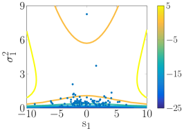
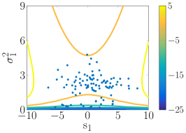
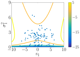
(a) Analytical method

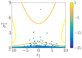
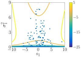
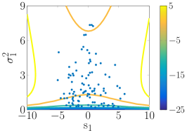
(b) Grid method

Figure 3: Linear-Gaussian problem: contours represent $\widetilde{J}_{1}(x_{1})$ and blue points are the regression points used to build these value function approximations. The left, middle, and right columns correspond to $\ell=1$, $2$, and $3$, respectively.

Note that the optimal policy is not unique for this problem, as there is a natural notion of exchangeability between the two designs $d_{0}$ and $d_{1}$. With no stage cost, the overall objective of this problem is the sum of the expected KL divergence and the expected distance of the final log-variance to the target log-variance. Both terms only depend on the final variance, which is determined exactly by the chosen values of $d_{k}$ through (15)—i.e., independently of the observations $y_{k}$. This phenomenon is particular to the linear-Gaussian problem with constant $\sigma_{\epsilon}^{2}$: the design problem is in fact deterministic, as the final variance is independent of the realized values of $y_{k}$. The optimal policy is then reducible to a choice of scalar-valued optimal designs $d_{0}^{\ast}$ and $d_{1}^{\ast}$. In other words, batch design will produce the same optimal designs as sOED for such deterministic problems since feedback does not add any design-relevant information. Moreover, we can find the exact optimal designs and expected reward function analytically in this problem; a derivation is given in Appendix B of [33]. Figure 4 plots the exact expected reward function over the design space, and overlays pairwise scatter plots of $(d_{0},d_{1})$ from 1000 trajectories simulated with the numerically-obtained sOED policy. The dotted black line represents the locus of exact optimal designs. The symmetry between the two experiments is evident, and the optimizer may hover around different parts of the optimal locus in different cases. The expected reward is relatively flat around the optimal design contour, however, and thus all these methods perform well. Histograms of total reward and their means from the 1000 trajectories are presented in Figure 5 and Table 1. The exact optimal reward value is $U(\pi^{\ast})\approx 0.7833$; the numerical sOED approaches agree with this value very closely, considering the Monte Carlo standard error. In contrast, the exploration policy produces a much lower expected reward of $U(\pi^{\textrm{explore}})=-8.5$.

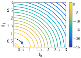
(a) Analytical method

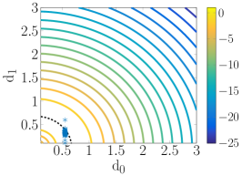
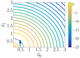
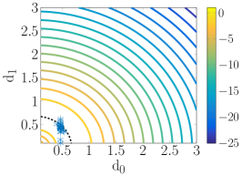
(b) Grid method

Figure 4: Linear-Gaussian problem: scatter plots of design pairs $(d_{0},d_{1})$ from 1000 simulated trajectories, superimposed on contours of the exact expected reward function. The black dotted line is the locus of exact optimal designs, obtained analytically. The left, middle, and right columns correspond to $\ell=1$, 2, and 3, respectively.

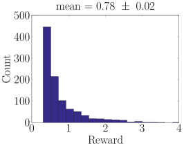
(a) Analytical method

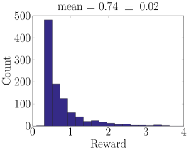
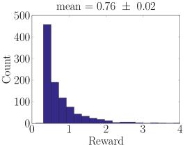
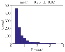
(b) Grid method

Figure 5: Linear-Gaussian problem: total reward histograms from 1000 simulated trajectories. The left, middle, and right columns correspond to $\ell=1$, 2, and 3, respectively.

Table 1: Linear-Gaussian problem: expected reward values (mean values of histograms in Figure 5) from 1000 simulated trajectories. Monte Carlo standard errors are all $\pm 0.02$. The true optimal expected reward is $\approx 0.7833$.

	$\ell=1$	$\ell=2$	$\ell=3$
Analytical	0.77	0.78	0.78
Grid	0.74	0.76	0.75

In summary, we have shown agreement between numerical sOED results and the true optimal design. Furthermore, we have demonstrated agreement between the analytical and grid-based methods of representing the belief state and performing inference, thus establishing credibility of the grid-based method for the subsequent nonlinear and non-Gaussian example, where an exact representation of the belief state is no longer possible.

4.2 Contaminant source inversion problem

Consider a situation where a chemical contaminant is accidentally released into the air. The contaminant plume diffuses and is advected by the wind. It is crucial to infer the location of the contaminant source so that an appropriate response can be undertaken. Suppose that an aerial or ground-based vehicle is dispatched to measure contaminant concentrations at a sequence of different locations, under a fixed time schedule. We seek the optimal policy for deciding where the vehicle should take measurements in order to maximize expected information gain in the source location. Our sOED problem will also account for hard constraints on possible vehicle movements, as well movement costs incorporated into the stage rewards.

We use the following simple plume model of the contaminant concentration at location $z$ and time $t$, given source location $\theta$:

$$G(\theta,z,t)=\frac{s}{\sqrt{2\pi}\left(\sqrt{1.2+4Dt}\right)}\exp\left(-\frac{\left\|\,\theta+d_{w}(t)-z\,\right\|^{2}}{2(1.2+4Dt)}\right),$$ (16)

where $s$, $D$, and $d_{w}(t)$ are the known source intensity, diffusion coefficient, and cumulative net displacement due to wind up to time $t$, respectively. The displacement $d_{w}(t)$ depends on the time history of the wind velocity. (Values of these coefficients will be specified later.) A total of $N$ measurements are performed, at uniformly spaced times given by $t=k+1$. (While $t$ is a continuous variable, we assume it to be suitably scaled so that it corresponds to the experiment index in this fashion; hence, observation $y_{0}$ is taken at $t=1$, $y_{1}$ at $t=2$, etc.) The state $x_{k}$ is a combination of a belief state and a physical state. Because an exact parametric representation of the posterior is not available in this nonlinear problem, the belief state is represented by an adaptive discretization of the posterior probability density function, using 100 nodes. The relevant physical state is the current location of the vehicle, i.e., $x_{k,p}=z$. Inclusion of physical state is necessary since the optimal design is expected to depend on the vehicle position as well as the belief state. Here we will consider the source inversion problem in one spatial dimension, where $\theta$, $d_{k}$, and $x_{k,p}$ are scalars (i.e., the plume and vehicle are confined to movements in a line). The design variables themselves correspond to the spatial displacement of the vehicle from one measurement time to the next. To introduce limits on the range of the vehicle, we use the box constraint $d_{k}\in[-d_{L},d_{R}]$, where $d_{L}$ and $d_{R}$ are bounds on the leftwards and rightwards displacement. The physical state dynamics then simply describe position and displacement: $x_{k+1,p}=x_{k,p}+d_{k}$.

The concentration measurements are corrupted by additive Gaussian noise:

$$y_{k}=G(\theta,x_{k+1,p},k+1)+\epsilon_{k}(x_{k},d_{k}),$$ (17)

where the noise $\epsilon_{k}\sim\mathcal{N}(0,\sigma_{\epsilon_{k}}^{2}(x_{k},d_{k}))$ may depend on the state and the design. When simulating a trajectory, the physical state must first be propagated before an observation $y_{k}$ can be generated, since the latter requires the evaluation of $G$ at $x_{k+1,p}$. Once $y_{k}$ is obtained, the belief state can then be propagated forward via Bayesian inference.

The reward functions used in this problem are

$$g_{k}(x_{k},y_{k},d_{k}) = -c_{b}-c_{q}|{d_{k}}|^{2},\ \text{and}$$

$$g_{N}(x_{N}) = D_{\mathrm{KL}}(f_{\theta|I_{N}}||f_{\theta|I_{0}}),$$

for $k=0,\ldots,N-1$. The terminal reward is simply the KL divergence, and the stage reward consists of a base cost of operation plus a penalty that is quadratic in the vehicle displacement.

We study three different cases of the problem, as described at the start of Section 4. Problem and algorithm settings common to all cases can be found in Tables 2 and 3, and additional variations will be described separately.

Table 2: Contaminant source inversion problem: problem settings.

Prior on $\theta$	$\mathcal{N}(0,2^{2})$
Design constraints	$d_{k}\in\left[-3,3\right]$
Initial physical state	$x_{0,p}=5.5$
Concentration strength	$s=30$
Diffusion coefficient	$D=0.1$
Base operation cost	$c_{b}=0.1$
Quadratic movement cost coefficient	$c_{q}=0.1$

Table 3: Contaminant source inversion problem: algorithm settings.

Number of grid points	100
Design measure for exploration policy	$d_{k}\sim\mathcal{N}(0,2^{2})$
Total number of regression points	500
% of regression points from exploration	30%
Maximum number of optimization iterations	50
Monte Carlo sample size in stochastic optimization	100

4.2.1 Case 1: comparison with greedy (myopic) design

This case highlights the advantage of sOED over greedy design, which is accentuated when future factors are important to the design of the current experiments. sOED will allow for coordination between subsequent experiments in a way that greedy design does not. We illustrate this idea via the wind factor: the air is calm initially, and then a constant wind of velocity 10 commences at $t=1$, leading to the following net displacement due to the wind up to time $t$:

$$d_{w}(t)=\left\{\begin{array}[]{cc}0,&t<1\\ 10(t-1),&t\geq 1\end{array}\right..$$ (20)

Consider $N=2$ experiments. Greedy design, by construction, chooses the first design to yield the single best experiment at $t=1$. This experiment is performed before plume has been advected. sOED, along with batch design, can take advantage of the fact that the plume will have moved by the second experiment, and make use of this knowledge even when designing the first experiment.

Details of the problem setup and numerical solution are as follows. The observation noise variance is set to $\sigma_{\epsilon_{k}}^{2}=4$ for all experiments. Features for the representation of the value function are analogous to those used in the previous example but now include the physical state as well: that is, we use polynomials up to total degree two in the posterior mean, posterior log-variance, and physical state (including cross-terms). Posterior moments are evaluated by trapezoidal rule integration on the adaptive grid. The terminal KL divergence is approximated by first estimating the mean and variance, and then applying the analytical formula for KL divergence between the associated Gaussian approximations. sOED uses $L=3$ policy updates, with a design measure for exploration of $d_{k}\sim\mathcal{N}(0,2^{2})$. Policies are compared by applying each to 1000 simulated trajectories, as summarized in Algorithm 2. The common assessment framework for this problem is a high-resolution grid discretization of the posterior probability density function with 1000 nodes.

Before presenting the results, we first provide some intuition for the progression of a single example trajectory, as shown in Figure 6. Suppose that a true value $\theta^{\ast}$ of the source location has been fixed (or sampled from the prior). The horizontal axis of the left figure corresponds to the physical space, with the vehicle starting at the location marked by the black square. To perform the first experiment, the vehicle moves to a new location and acquires the noisy observation indicated by the blue cross, with the solid blue curve indicating the plume profile $G(\theta^{\ast},z,t=1)$ at that time. For the second experiment, the vehicle moves to another location and acquires the noisy observation indicated by the red cross; the dotted red curve shows the plume profile $G(\theta^{\ast},z,t=2)$, which has diffused slightly and been carried to the right by the wind. The right figure shows the corresponding belief state (i.e., posterior density) at each stage. Starting from the solid blue prior density, the posterior density after the first experiment (dashed red) narrows only slightly, since the first observation is in a region dominated by measurement noise. The posterior after both experiments (dotted yellow), however, becomes much narrower, as the second observation is in a high-gradient region of the concentration profile and thus carries significant information for identifying $\theta$. The posteriors in this problem can become quite non-Gaussian and even multimodal. The black circle in Figure 6(b) indicates the true value of $\theta$; the posterior mode after the second experiment is close to this value but should not be expected to match it exactly, due to noisy measurements and the finite number of observations.

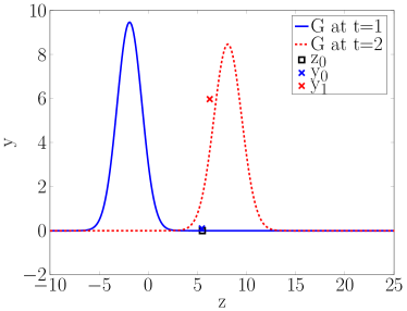
(a) Physical state and plume profiles

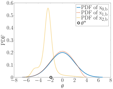
(b) Belief state, i.e., probability densities of $\theta$.

Figure 6: Contaminant source inversion problem, Case 1: progression of the physical state and belief state for a sample trajectory.

Now we compare results of the greedy and sOED policies. Only data from $\ell=3$ are shown for sOED, as other iterations produced similar results. Pairwise scatter plots of the generated designs $(d_{0},d_{1})$ for 1000 simulated trajectories are shown in Figure 7. Greedy designs generally move towards the left for the first experiment (negative values of $d_{0}$) since for almost all prior realizations of $\theta$, the bulk of the plume is to the left of the initial vehicle location. When designing the first experiment, greedy design by construction does not account for the fact that there will be a second experiment and that the wind will eventually blow the plume to the right; thus it moves the vehicle to the left in order to acquire information immediately. Similarly, when designing the second experiment, the greedy policy chases after the plume, which is now to the right of the vehicle; hence we see positive values of $d_{1}$. sOED, however, generally starts moving the vehicle to the right for the first experiment, so that it can arrive in the regions of highest information gain (which correspond to high expected gradient of the concentration field) in time for the second experiment, after the plume has been carried by the wind. Both policies produce a few cases where $d_{1}$ is very close to zero, however. These cases correspond to samples of $\theta$ drawn from the right tail of the prior, making the plume much closer to the initial vehicle location. As a result, a large amount of information is obtained from the first observation. The plume is subsequently carried 10 units to the right by the wind, and the vehicle cannot reach regions that yield sufficiently high information gain from the second experiment to justify the movement cost for $d_{1}$. The best action is then to simply stay put, leading to these near-zero $d_{1}$ values. Note that these small-$d_{1}$ cases are very much the result of feedback from the first experiment, which would not be available in a batch experimental design setting.

Overall, the tendency of the greedy design policy to “chase” high-information experimental configurations turns out to be costly due to the quadratic movement penalty. This cost is reflected in Figure 8, which shows histograms of total reward from the trajectories. sOED yields an expected reward of $U(\pi^{L})=0.15\pm 0.02$, whereas greedy produces a lower value of $U(\pi^{\text{greedy}})=0.07\pm 0.02$; the plus-minus quantity is the Monte Carlo standard error.

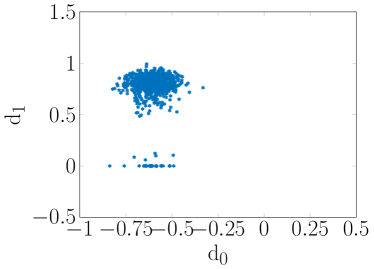
(a) Greedy design

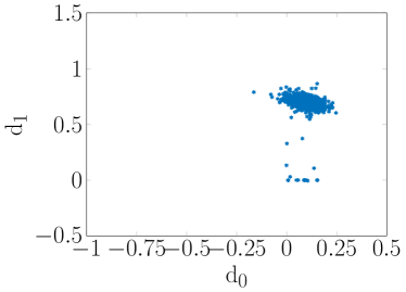
(b) sOED

Figure 7: Contaminant source inversion problem, Case 1: scatter plots of $(d_{0},d_{1})$ from 1000 simulated trajectories for the greedy and sOED policies.

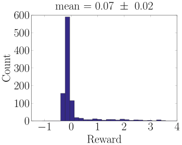
(a) Greedy design

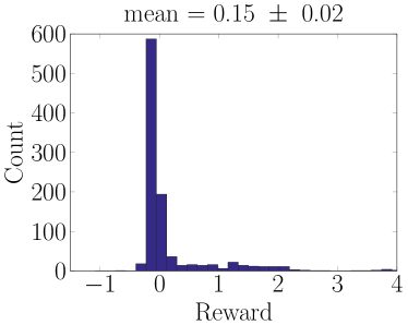
(b) sOED

Figure 8: Contaminant source inversion problem, Case 1: histograms of total reward from 1000 simulated trajectories for greedy design and sOED.

4.2.2 Case 2: comparison with batch (open-loop) design

This case highlights the advantage of sOED over batch design, which is accentuated when useful information for designing experiments can be obtained by performing some portion of the experiments first (i.e., by allowing feedback). Again consider $N=2$ experiments. We illustrate the impact of feedback via a scenario involving two different measurement devices: suppose that the vehicle carries a “coarse” sensor with an observation noise variance of $\sigma^{2}_{\epsilon_{k}}=4$ and a “precise” sensor with $\sigma^{2}_{\epsilon_{k}}=0.25$. Suppose also that the precise sensor is a scarce resource, and can only be utilized when there is a good chance of localizing the source; in particular, rules require it to be used if and only if the current posterior variance is below a threshold of 3. (Recall that the prior variance is 4.) The observation noise standard deviation thus has the form

$$\sigma_{\epsilon_{k}}^{2}(x_{k,b})=\left\{\begin{array}[]{cc}0.25,&\textrm{if \{variance corresponding to }x_{k,b}\}<3\\ 4,&\textrm{otherwise}\end{array}\right..$$ (23)

The same wind conditions as in (20) are applied. Batch design is expected to perform poorly for this case, since it cannot include the effect of feedback in its assessment of different experimental configurations, and thus cannot plan for the use of the precise sensor.

The same numerical setup as Case 1 is used. Policies are assessed using the same procedure but with one caveat. Batch design selected $d_{0}$ and $d_{1}$ without accounting for feedback from the result of the first experiment. But in assessing the performance of the optimal batch design, we will allow the belief state to be updated between experiments; this choice maintains a common assessment framework between the batch and sOED design strategies, and is in fact more favorable to batch design than a feedback-free assessment. In particular, updating the belief state permits the use of the precise sensor. In other words, while batch design cannot strategically plan for the use of the precise sensor, we make this sensor available in the policy assessment stage if the condition in (23) is satisfied.

Again, only data from $\ell=3$ for sOED are shown, with other iterations producing similar results. Pairwise scatter plots of $(d_{0},d_{1})$ for 1000 simulated trajectories are shown in Figure 9. As expected, batch design is able to account for change in wind velocity at $t=1$ and immediately starts moving the vehicle to the right for the first experiment so that it can reach locations of higher information gain for the second experiment, after the plume is advected to the right. sOED, however, realizes that there is the possibility of using the precise device in the second experiment if it can reduce the posterior variance below the threshold using the first observation. Thus it moves to the left in the first experiment (towards the more likely initial plume locations) to obtain an observation that is expected to be more informative, even though the movement cost is higher. This behavior is in stark contrast with that of the sOED policy for Case 1. Roughly 55% of the resulting sOED trajectories achieve the threshold for using the precise device in the second experiment compared to only 8% from batch design. This subset of the sOED trajectories has an expected reward of $U=0.51$, in contrast to $U=-0.01$ for the subset of trajectories that fail to qualify. Effectively, the sOED policy creates an opportunity for a much larger reward with a slightly higher cost of initial investment. Histograms of the total rewards from all 1000 trajectories are shown in Figure 8. Indeed, the reward distribution for the sOED policy sees more mass in higher values. Overall the risk taken by sOED pays off as it produces an expected reward of $U(\pi^{L})=0.26\pm 0.02$, while batch design produces a much lower value of $U(\pi^{\text{batch}})=0.15\pm 0.02$.

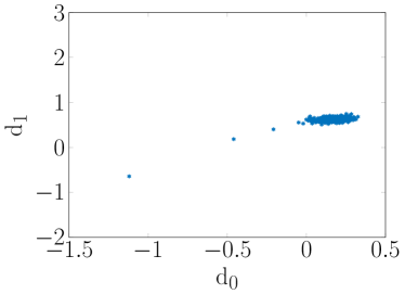
(a) Batch design

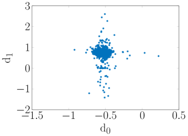
(b) sOED

Figure 9: Contaminant source inversion problem, Case 2: scatter plots of $(d_{0},d_{1})$ from 1000 simulated trajectories of batch design and sOED.

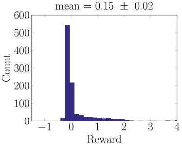
(a) Batch design

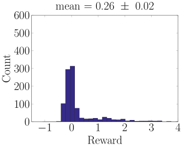
(b) sOED

Figure 10: Contaminant source inversion problem, Case 2: histograms of total reward from 1000 simulated trajectories of batch design and sOED.

4.2.3 Case 3: additional experiments and policy updates

This case demonstrates sOED with a larger number of experiments, and also explores the ability of our policy update mechanism to improve the policy resulting from a poor initial choice of design measure for exploration. We consider $N=4$ experiments, with the wind condition

$$d_{w}(t)=\left\{\begin{array}[]{cc}0,&t<1\\ 5(t-1),&t\geq 1\end{array}\right.,$$ (26)

and a two-tiered measurement system similar to that of Case 2:

$$\sigma_{\epsilon_{k}}^{2}(x_{k,b})=\left\{\begin{array}[]{cc}0.25,&\textrm{if \{variance corresponding to }x_{k,b}\}<2.5\\ 4,&\textrm{otherwise}\end{array}\right..$$ (29)

A total of $L=10$ policy updates are conducted, starting with a design measure for exploration of $\mathcal{N}(-2.5,0.1)$, which targets a particular point in the left part of design space and ignores the remaining regions. Subsequent iterations use a mix of 5% exploration and 95% exploitation trajectories as regression points. 100-node grids are used both to construct the policy and to drive the common assessment framework. All other settings remain the same as in Cases 1 and 2. For this case, we intuitively expect the most informative data (and the most design “activity,” i.e., variation in policy outputs) to occur at the second and third experiments, as the plume is carried by the wind through the vehicle starting location ($x_{0,p}=5.5$) at those times. Additionally, we anticipate that the advantage of the precise instrument might be less prominent compared to Case 2, since more experiments are performed overall.

Figure 11 presents distributions of each design $d_{k}$ (drawn sideways) from 1000 simulated trajectories versus the policy update index, $\ell$. The blue dashed line connects the mean values of successive distributions. Figure 12 shows a similar plot for the total reward, with expected rewards also reported in Table 4. We can immediately make two observations. First, the policy at $\ell=1$ appears to be quite poor, producing an expected reward that is significantly lower than that of subsequent iterations. This low value is to be expected, given the poor initial choice of design measure for exploration. Starting at $\ell=2$, exploitation samples become available for regression, and they contribute to a dramatic improvement in the expected reward. (Under the hood, this jump corresponds to a significant improvement in the value function approximations $\widetilde{J}_{k}$.) Large differences between the $d_{k}$ distributions of these first two iterations can also be observed. In comparison, subsequent iterations show much smaller changes; this is consistent with the intuition described in Section 3.2.3.

Second, a small oscillatory behavior can be seen between iterations, most visibly in $d_{0}$. This is likely due to some interaction between the limitations of the selected features in capturing the landscape of the true value function, and the ensuing locations of the regression points generated by exploration. In other words, the regression points might oscillate slightly around the region of the state space visited by the optimal policy. Nonetheless, the design oscillations are quite small compared to the first change following $\ell=1$. The oscillations are also small relative to the range of the overall design space and the width of the design distributions. More importantly, an oscillation is not visible in the reward distributions of Figure 12 and in the values of the expected reward, implying a sense of “flatness” around the optimal policy.

We also performed numerical tests on this problem using a more reasonable design measure for exploration of $\mathcal{N}(0,4)$, with 30% exploration samples; results are reported in Table 5. The expected reward values from $\ell=1$ and from the pure exploration policy are much better compared to their counterparts in Table 4.

Overall, these results indicate that the first iteration of policy update (from $\ell=1$ to $\ell=2$) can be very helpful, especially when it is unclear what a suitable design measure for exploration should be. This first iteration can help recover from extremely poor initial choices of exploration policy. Subsequently, it seems that only a small number of policy updates (e.g., $L=3$) are needed in practice.

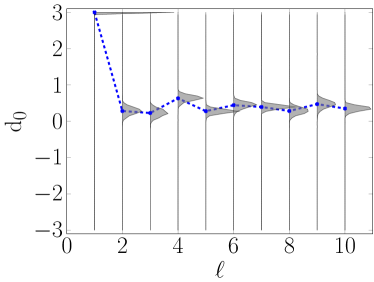
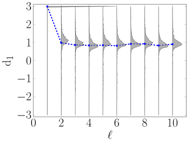
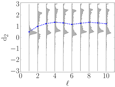
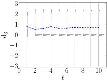
Figure 11: Contaminant source inversion problem, Case 3: design distributions for $d_{0}$, $d_{1}$, $d_{2}$, and $d_{3}$, from 1000 simulated trajectories over successive steps $\ell$ of policy update. The blue dashed line connects the means of the distributions.

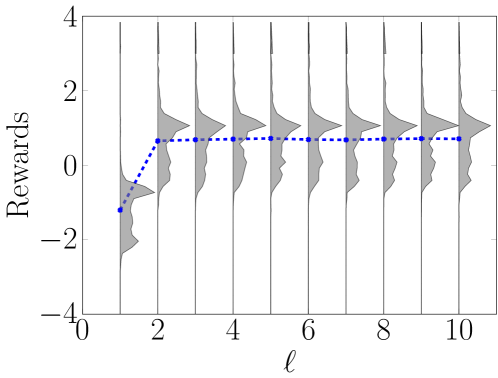
Figure 12: Contaminant source inversion problem, Case 3: distributions of total reward following $N=4$ experiments, from 1000 simulated trajectories over successive steps $\ell$ of policy update. The blue dashed line connects the means of distributions. Mean values are also given in Table 4.

Table 4: Contaminant source inversion problem, Case 3: expected rewards (mean values of histograms in Figure 12) estimated from 1000 simulated trajectories, using a “poor” design measure for exploration of $\mathcal{N}(-2.5,0.1)$.

$\ell$	Expected reward	$\ell$	Expected reward
1	$-1.20\pm 0.02$	6	$0.69\pm 0.03$
2	$0.65\pm 0.03$	7	$0.68\pm 0.03$
3	$0.68\pm 0.02$	8	$0.70\pm 0.03$
4	$0.70\pm 0.02$	9	$0.71\pm 0.02$
5	$0.72\pm 0.03$	10	$0.71\pm 0.03$
Exploration	$-2.00\pm 0.03$

Table 5: Contaminant source inversion problem, Case 3: expected rewards, estimated from 1000 simulated trajectories, using a “better” design measure for exploration of $\mathcal{N}(0,4)$.

$\ell$	Expected reward
1	$0.67\pm 0.02$
2	$0.65\pm 0.03$
3	$0.68\pm 0.03$
Exploration	$-0.70\pm 0.03$

5 Conclusions

We have developed a rigorous formulation of the sequential optimal experimental design (sOED) problem, in a fully Bayesian and decision-theoretic setting. The solution of the sOED problem is not a set of designs, but rather a feedback control policy—i.e., a decision rule that specifies which experiment to perform as a function of the current system state. The latter incorporates the current posterior distribution (i.e., belief state) along with any other design-relevant variables. More commonly-used batch and greedy experimental design approaches are shown to result from simplifications of this sOED formulation; these approaches are in general suboptimal. Unlike batch or greedy design alone, sOED combines coordination among multiple experiments, which includes the ability to account for future effects, with feedback, where information derived from each experiment influences subsequent designs.

Directly solving for the optimal policy is a challenging task, particularly in the setting considered here: a finite horizon of experiments, described by continuous parameter, design, and observation spaces, with nonlinear models and non-Gaussian posterior distributions. Instead we cast the sOED problem as a dynamic program and employ various approximate dynamic programming (ADP) techniques to approximate the optimal policy. Specifically, we use a one-step lookahead policy representation, combined with approximate value iteration (backward induction with regression). Value functions are approximated using a linear architecture and estimated via a series of regression problems obtained from the backward induction procedure, with regression points generated via both exploration and exploitation. In obtaining good regression samples, we emphasize the notion of the state measure induced by the current policy; our algorithm incorporate an update to adapt and refine this measure as better policy approximations are constructed.

We apply our numerical ADP approach to several examples of increasing complexity. The sOED policy is first verified on a linear-Gaussian problem, where an exact solution is available analytically. The methods are then tested on a nonlinear and time-dependent contaminant source inversion problem. Different test cases demonstrate the advantages of sOED over batch and greedy design, and the ability of policy update to improve the initial policy resulting from a poor choice of design measure for exploration.

There remain many important avenues for future work. One challenge involves the representation of the belief state $x_{k,b}$, and the associated inference methodologies. The ADP approaches developed here are largely agnostic to the representation of the belief state: as long as one can evaluate the system dynamics $x_{k+1}=\mathcal{F}_{k}(x_{k},y_{k},d_{k})$ and the features $\phi_{k,i}(x_{k})$, then approximate value iteration and all the other elements of our ADP algorithm can be directly applied. In the case of parametric posteriors (e.g., Bayesian inference with conjugate priors and likelihoods) the representation and updating of $x_{k,b}$ is trivial. But in the general case of continuous and non-Gaussian posteriors, finding an efficient representation of $x_{k,b}$—one that allows repeated inference under different realizations of the data—can be difficult. In this paper, we have employed an adaptive discretization of the posterior probability density function, but this choice is impractical for higher parameter dimensions. A companion paper will explore a more flexible and scalable alternative, based on the construction of transport maps over the joint distribution of parameters and data, from which conditionals can efficiently be extracted [49, 45]. Alternative ADP approaches are also of great interest, including model-free methods such as $Q$-learning.

References

- [1] A. Alexanderian, N. Petra, G. Stadler, and O. Ghattas, A Fast and Scalable Method for A-Optimal Design of Experiments for Infinite-Dimensional Bayesian Nonlinear Inverse Problems, (2014), arXiv:1410.5899.
- [2] A. C. Atkinson and A. N. Donev, Optimum Experimental Designs, Oxford University Press, New York, NY, 1992.
- [3] R. Bellman, Bottleneck Problems and Dynamic Programming, Proc. Natl. Acad. Sci. U. S. A., 39 (1953), pp. 947–951, http://dx.doi.org/10.1073/pnas.39.9.947.
- [4] R. Bellman, Dynamic Programming and Lagrange Multipliers, Proc. Natl. Acad. Sci. U. S. A., 42 (1956), pp. 767–769, http://dx.doi.org/10.1073/pnas.42.10.767.
- [5] I. Ben-Gal and M. Caramanis, Sequential DOE via dynamic programming, IIE Trans. (Institute Ind. Eng., 34 (2002), pp. 1087–1100, http://dx.doi.org/10.1023/A:1019670414725.
- [6] J. O. Berger, Statistical Decision Theory and Bayesian Analysis, Springer New York, New York, NY, 1985, http://dx.doi.org/10.1007/978-1-4757-4286-2.
- [7] D. A. Berry, P. Müller, A. P. Grieve, M. Smith, T. Parke, R. Blazek, N. Mitchard, and M. Krams, Adaptive Bayesian Designs for Dose-Ranging Drug Trials, in Case Stud. Bayesian Stat., Springer New York, New York, NY, 2002, pp. 99–181, http://dx.doi.org/10.1007/978-1-4613-0035-9_2.
- [8] D. P. Bertsekas, Dynamic Programming and Optimal Control, Vol. 1, Athena Scientific, Belmont, MA, 2005.
- [9] D. P. Bertsekas, Dynamic Programming and Optimal Control, Vol. 2, Athena Scientific, Belmont, MA, 2007.
- [10] D. P. Bertsekas and S. E. Shreve, Stochastic Optimal Control, Athena Scientific, Belmont, MA, 1996.
- [11] D. P. Bertsekas and J. N. Tsitsiklis, Neuro-Dynamic Programming, Athena Scientific, Belmont, MA, 1996.
- [12] F. Bisetti, D. Kim, O. Knio, Q. Long, and R. Tempone, Optimal Bayesian experimental design for priors of compact support with application to shock-tube experiments for combustion kinetics, Int. J. Numer. Methods Eng., (2016), pp. 1–19, http://dx.doi.org/10.1002/nme.5211.
- [13] G. E. P. Box and N. R. Draper, Empirical Model-Building and Response Surfaces, John Wiley & Sons, Hoboken, NJ, 1987.
- [14] G. E. P. Box, J. S. Hunter, and W. G. Hunter, Statistics for Experimenters: Design, Innovation and Discovery, John Wiley & Sons, Hoboken, NJ, 2nd ed., 2005.
- [15] A. E. Brockwell and J. B. Kadane, A Gridding Method for Bayesian Sequential Decision Problems, J. Comput. Graph. Stat., 12 (2003), pp. 566–584, http://dx.doi.org/10.1198/1061860032274.
- [16] P. Carlin, Bradley, J. B. Kadane, and A. E. Gelfand, Approaches for Optimal Sequential Decision Analysis in Clinical Trials, Biometrics, 54 (1998), pp. 964–975, http://dx.doi.org/10.2307/2533849.
- [17] D. R. Cavagnaro, J. I. Myung, M. A. Pitt, and J. V. Kujala, Adaptive Design Optimization: A Mutual Information-Based Approach to Model Discrimination in Cognitive Science, Neural Comput., 22 (2010), pp. 887–905, http://dx.doi.org/10.1162/neco.2009.02-09-959.
- [18] K. Chaloner and I. Verdinelli, Bayesian Experimental Design: A Review, Stat. Sci., 10 (1995), pp. 273–304, http://dx.doi.org/10.1214/ss/1177009939.
- [19] J. A. Christen and M. Nakamura, Sequential Stopping Rules for Species Accumulation, J. Agric. Biol. Environ. Stat., 8 (2003), pp. 184–195, http://dx.doi.org/10.1198/108571103322161540.
- [20] T. A. Cover and J. A. Thomas, Elements of Information Theory, John Wiley & Sons, Hoboken, NJ, 2nd ed., 2006.
- [21] D. R. Cox and N. Reid, The Theory of the Design of Experiments, Chapman & Hall/CRC, Boca Raton, FL, 2000.
- [22] H. A. Dror and D. M. Steinberg, Sequential Experimental Designs for Generalized Linear Models, J. Am. Stat. Assoc., 103 (2008), pp. 288–298, http://dx.doi.org/10.1198/016214507000001346.
- [23] C. C. Drovandi, J. M. McGree, and A. N. Pettitt, Sequential Monte Carlo for Bayesian sequentially designed experiments for discrete data, Comput. Stat. Data Anal., 57 (2013), pp. 320–335, http://dx.doi.org/10.1016/j.csda.2012.05.014.
- [24] C. C. Drovandi, J. M. McGree, and A. N. Pettitt, A Sequential Monte Carlo Algorithm to Incorporate Model Uncertainty in Bayesian Sequential Design, J. Comput. Graph. Stat., 23 (2014), pp. 3–24, http://dx.doi.org/10.1080/10618600.2012.730083.
- [25] T. A. El Moselhy and Y. M. Marzouk, Bayesian inference with optimal maps, J. Comput. Phys., 231 (2012), pp. 7815–7850, http://dx.doi.org/10.1016/j.jcp.2012.07.022.
- [26] V. V. Fedorov, Theory of Optimal Experiments, Academic Press, New York, NY, 1972.
- [27] R. A. Fisher, The Design of Experiments, Oliver & Boyd, Edinburgh, United Kingdom, 8th ed., 1966.
- [28] S. Fujishige, Submodular Functions and Optimization, Elsevier, Amsterdam, The Netherlands, 2nd ed., 2005, http://dx.doi.org/10.1016/S0167-5060(05)80003-2.
- [29] J. Ginebra, On the Measure of the Information in a Statistical Experiment, Bayesian Anal., 2 (2007), pp. 167–212, http://dx.doi.org/10.1214/07-BA207.
- [30] G. J. Gordon, Stable Function Approximation in Dynamic Programming, in Proc. 12th Int. Conf. Mach. Learn., Tahoe City, CA, 1995, pp. 261–268, http://dx.doi.org/10.1016/b978-1-55860-377-6.50040-2.
- [31] I. Guyon, M. Nikravesh, S. Gunn, and L. A. Zadeh, Feature Extraction: Foundations and Applications, Springer Berlin Heidelberg, Berlin, Germany, 2006, http://dx.doi.org/10.1007/978-3-540-35488-8.
- [32] E. Haber, L. Horesh, and L. Tenorio, Numerical methods for the design of large-scale nonlinear discrete ill-posed inverse problems, Inverse Probl., 26 (2010), p. 025002, http://dx.doi.org/10.1088/0266-5611/26/2/025002.
- [33] X. Huan, Numerical Approaches for Sequential Bayesian Optimal Experimental Design, PhD thesis, Massachusetts Institute of Technology, 2015.
- [34] X. Huan and Y. M. Marzouk, Simulation-based optimal Bayesian experimental design for nonlinear systems, J. Comput. Phys., 232 (2013), pp. 288–317, http://dx.doi.org/10.1016/j.jcp.2012.08.013.
- [35] X. Huan and Y. M. Marzouk, Gradient-Based Stochastic Optimization Methods in Bayesian Experimental Design, Int. J. Uncertain. Quantif., 4 (2014), pp. 479–510, http://dx.doi.org/10.1615/Int.J.UncertaintyQuantification.2014006730.
- [36] L. P. Kaelbling, M. L. Littman, and A. W. Moore, Reinforcement Learning: A Survey, J. Artif. Intell. Res., 4 (1996), pp. 237–285, http://dx.doi.org/10.1613/jair.301.
- [37] W. Kim, M. A. Pitt, Z.-L. Lu, M. Steyvers, and J. I. Myung, A Hierarchical Adaptive Approach to Optimal Experimental Design, Neural Comput., 26 (2014), pp. 2565–2492, http://dx.doi.org/10.1162/NECO_a_00654.
- [38] A. Krause, A. Singh, and C. Guestrin, Near-Optimal Sensor Placements in Gaussian Processes: Theory, Efficient Algorithms and Empirical Studies, J. Mach. Learn. Res., 9 (2008), pp. 235–284, http://dx.doi.org/10.1145/1102351.1102385.
- [39] M. Lagoudakis, Least-Squares Policy Iteration, J. Mach. Learn. Res., 4 (2003), pp. 1107–1149.
- [40] D. V. Lindley, On a Measure of the Information Provided by an Experiment, Ann. Math. Stat., 27 (1956), pp. 986–1005, http://dx.doi.org/10.1214/aoms/1177728069.
- [41] H. Liu and H. Motoda, Feature Selection for Knowledge Discovery and Data Mining, Springer US, New York, NY, 1998, http://dx.doi.org/10.1007/978-1-4615-5689-3.
- [42] Q. Long, M. Scavino, R. Tempone, and S. Wang, Fast estimation of expected information gains for Bayesian experimental designs based on Laplace approximations, Comput. Methods Appl. Mech. Eng., 259 (2013), pp. 24–39, http://dx.doi.org/10.1016/j.cma.2013.02.017.
- [43] T. J. Loredo, Rotating Stars and Revolving Planets: Bayesian Exploration of the Pulsating Sky, in Bayesian Stat. 9 Proc. Nineth Val. Int. Meet., Benidorm, Spain, 2010, pp. 361–392, http://dx.doi.org/10.1093/acprof:oso/9780199694587.003.0012.
- [44] D. J. C. MacKay, Information Theory, Inference, and Learning Algorithms, Cambridge University Press, Cambridge, United Kingdom, 4th ed., 2005, http://dx.doi.org/10.1198/jasa.2005.s54.
- [45] Y. M. Marzouk, T. A. El Moselhy, M. D. Parno, and A. Spantini, An introduction to sampling via measure transport, in Handb. Uncertain. Quantif., Springer International Publishing, 2016.
- [46] P. Müller, D. A. Berry, A. P. Grieve, M. Smith, and M. Krams, Simulation-based sequential Bayesian design, J. Stat. Plan. Inference, 137 (2007), pp. 3140–3150, http://dx.doi.org/10.1016/j.jspi.2006.05.021.
- [47] S. A. Murphy, Optimal dynamic treatment regimes, J. R. Stat. Soc. Ser. B (Statistical Methodol., 65 (2003), pp. 331–355, http://dx.doi.org/10.1111/1467-9868.00389.
- [48] D. Ormoneit and Ś. Sen, Kernel-Based Reinforcement Learning, Mach. Learn., 49 (2002), pp. 161–178, http://dx.doi.org/10.1023/A:1017928328829.
- [49] M. Parno and Y. Marzouk, Transport map accelerated Markov chain Monte Carlo, (2014), arXiv:1412.5492.
- [50] W. B. Powell, Approximate Dynamic Programming: Solving the Curses of Dimensionality, John Wiley & Sons, Hoboken, NJ, 2nd ed., 2011.
- [51] M. L. Puterman, Markov Decision Processes: Discrete Stochastic Dynamic Programming, John Wiley & Sons, Hoboken, NJ, 1994.
- [52] K. J. Ryan, Estimating Expected Information Gains for Experimental Designs With Application to the Random Fatigue-Limit Model, J. Comput. Graph. Stat., 12 (2003), pp. 585–603, http://dx.doi.org/10.1198/1061860032012.
- [53] O. Sigaud and O. Buffet, Markov Decision Processes in Artificial Intelligence: MDPs, beyond MDPs and applications, John Wiley & Sons, Hoboken, NJ, 2010, http://dx.doi.org/10.1002/9781118557426.
- [54] A. Solonen, H. Haario, and M. Laine, Simulation-Based Optimal Design Using a Response Variance Criterion, J. Comput. Graph. Stat., 21 (2012), pp. 234–252, http://dx.doi.org/10.1198/jcgs.2011.10070.
- [55] R. S. Sutton and A. G. Barto, Reinforcement Learning: An Introduction, The MIT Press, Cambridge, MA, 1998.
- [56] G. Terejanu, R. R. Upadhyay, and K. Miki, Bayesian experimental design for the active nitridation of graphite by atomic nitrogen, Exp. Therm. Fluid Sci., 36 (2012), pp. 178–193, http://dx.doi.org/10.1016/j.expthermflusci.2011.09.012.
- [57] J. N. Tsitsiklis and B. Van Roy, An Analysis of Temporal-Difference Learning with Function Approximation, IEEE Trans. Autom. Control (Institute Electr. Electron. Eng., 42 (1997), pp. 674–690, http://dx.doi.org/10.1109/9.580874.
- [58] J. N. Tsitsiklis and B. Van Roy, Regression Methods for Pricing Complex American-Style Options, IEEE Trans. Neural Networks (Institute Electr. Electron. Eng., 12 (2001), pp. 694–703, http://dx.doi.org/10.1109/72.935083.
- [59] C. Villani, Optimal Transport: Old and New, Springer-Verlag Berlin Heidelberg, Berlin, Germany, 2008.
- [60] U. Von Toussaint, Bayesian inference in physics, Rev. Mod. Phys., 83 (2011), pp. 943–999, http://dx.doi.org/10.1103/RevModPhys.83.943.
- [61] J. K. Wathen and J. A. Christen, Implementation of Backward Induction for Sequentially Adaptive Clinical Trials, J. Comput. Graph. Stat., 15 (2006), pp. 398–413, http://dx.doi.org/10.1198/016214506X113406.
- [62] C. J. C. H. Watkins, Learning from delayed rewards, PhD thesis, King’s College, 1989.
- [63] C. J. C. H. Watkins and P. Dayan, Technical Note: Q-Learning, Mach. Learn., 8 (1992), pp. 279–292, http://dx.doi.org/10.1023/a:1022676722315.
- [64] B. P. Weaver, B. J. Williams, C. M. Anderson-Cook, and D. M. Higdon, Computational Enhancements to Bayesian Design of Experiments Using Gaussian Processes, Bayesian Anal., (2015), http://dx.doi.org/10.1214/15-BA945.