Intermittency and Velocity Fluctuations in Hopper Flows Prone to Clogging
Abstract
We experimentally study the dynamics of granular media in a discharging hopper. In such flows, there often appears to be a critical outlet size such that the flow never clogs for . We report on the time-averaged velocity distributions, as well as temporal intermittency in the ensemble-averaged velocity of grains in a viewing window, for both and , near and far from the outlet. We characterize the velocity distributions by the standard deviation and the skewness of the distribution of vertical velocities. We propose a measure for intermittency based on the two-sample Kolmogorov-Smirnov -statistic for the velocity distributions as a function of time. We find that there is no discontinuity or kink in these various measures as a function of hole size. This result supports the proposition that there is no well-defined and that clogging is always possible. Furthermore, the intermittency time scale of the flow is set by the speed of the grains at the hopper exit. This latter finding is consistent with a model of clogging as the independent sampling for stable configurations at the exit with a rate set by the exiting grain speed [Thomas and Durian, Phys. Rev. Lett. (2015)].
I Introduction
The gravity-driven flow of grains in an hourglass or hopper is an iconic granular phenomenon. Fundamental issues of continued interest in granular physics today Duran (2000); Franklin and Shattuck (2016) include the shape of the coarse-grained velocity flow field Nedderman and Tüzün (1979); Tüzün and Nedderman (1979); Samadani et al. (1999); Choi et al. (2005); Garcimartín et al. (2011), the rate at which grains are discharged Beverloo et al. (1961); Nedderman et al. (1982); Mankoc et al. (2007); Aguirre et al. (2010); Hilton and Cleary (2011); Janda et al. (2012); Rubio-Largo et al. (2015); Dunatunga and Kamrin (2015), and the susceptibility of the system to clogging Manna and Herrmann (2000); To et al. (2001); Zuriguel et al. (2005); Janda et al. (2008); Mankoc et al. (2009); Sheldon and Durian (2010); Thomas and Durian (2013); Zuriguel (2014); Thomas and Durian (2015). The latter is usually quantified in terms of the average mass or number of grains that is discharged before a clog occurs. Experimentally, is found to grow very rapidly with increasing hole size and may be fit to a power-law divergence in order to locate a clogging transition. However, may also be fit equally well to an exponential function, in which case there is no actual transition and clogging is in principle possible for any hole size. If there truly is a transition, it ought to be possible to located it from above, i.e. by observing a critical change in some measured quantity as the hole size is decreased. To our knowledge this has not been accomplished. The closest is perhaps Ref. Sheldon and Durian (2010), where the nominal transition was bracketed by observing the stop and start angles at which a hopper with fixed hole size spontaneously clogs or unclogs as it is slowly tilted or untilted. However such experiments depend on tilting rate. Certainly, there is no discontinuity or kink in discharge rate versus hole size at the nominal transition Sheldon and Durian (2010); Thomas and Durian (2013).
The clogging transition, if it exists, is distinct from the jamming transition since the latter is for a spatially uniform system with no boundary effects. Nevertheless, it seems likely that grains on the verge of clogging could display similarities to grains on the verge of jamming. For example, there could be enhanced velocity fluctuations relative to the mean Menon and Durian (1997); Lemieux and Durian (2000a); Katsuragi et al. (2010), growing dynamical heterogeneities Berthier et al. (2011), or both Katsuragi et al. (2010) as the hole size is decreased toward the transition. A related but different question is to examine fluctuations versus time with a view toward predicting the imminence of clog formation for systems well within the clogging regime Tewari et al. (2013). Here we explore behavior versus outlet size experimentally for a quasi-2D system of grains confined between clear parallel plates separated by a distance of about ten grain diameters, where discharge happens through a narrow slit at the bottom of the sample that extends across the full distance between the plates. In particular, we use high-speed digital video particle-tracking techniques to measure fluctuations of the individual grain velocities, and intermittency of ensemble velocities, as a function of hole size both above and below the nominal clogging transition. The results show that hopper flows susceptible to clogging have elevated fluctuations and are more strongly intermittent. However, this intermittency does not possess a time scale other than that set by average flow speed and grain size, i.e. it grows smoothly as the hole size is decreased through the transition, without any evidence of criticality. This supports the notation that there is no actual well-defined clogging transition.
II Prior Experiments
Well-known phenomenon involving fluctuations in granular hopper flow include silo quaking and ticking. These are typically observed with cohesive grains Mersch et al. (2010) or where the interactions between the grains and the interstitial fluid Wu et al. (1993); Bertho et al. (2003) or the walls Börzsönyi and Kovács (2011) are particularly strong. Of more direct relevance for our work is study of intermittency in the mass discharge rate. For example, Uñac and co-workers found both fluctuations and characteristic time scales growing with decreasing hole size Uñac et al. (2012). However, Janda and co-authors found no such behavior Janda et al. (2009). Garcimartín and co-workers studied both the individual and ensemble velocity distributions as a function of hole size, but presented no systematic measurement of the fluctuation magnitude versus hole size Garcimartín et al. (2011). To our knowledge, the only peer-reviewed experimental work which explicitly reports on either the size of ensemble fluctuations or the time scale of the flow fluctuations throughout the bulk as a function of hole size is by Vivanco et al. for highly wedge-shaped hoppers Vivanco et al. (2012). While this is an important geometry, it is more complicated, as these hoppers exhibit anomalous clogging statistics Saraf and Franklin (2011). Thus there is need for the comprehensive characterization we report below.
III Experimental Methods
For our work we use a quasi-2D hopper constructed with smooth, transparent, static-dissipative side walls. The interior dimensions of the hopper are cm2, and it is typically filled to a height of at least 80 cm. In this experimental regime there is no filling-height dependence of the flow Nedderman et al. (1982). The orifice is a rectangular slit at the bottom of the hopper with adjustable width and constant length cm, running the full thickness of the hopper. The width of the slit, front and back, is measured with calipers both before and after experiments. In all cases the variation in the slit width is less than 0.1 mm. We fix dowels on the hopper floor at the edges of the opening to inhibit the sliding of grains along the bottom. As a model granular medium suitable for imaging, we use mm monodisperse dry tapioca pearls. These grains are large enough that friction and hard-sphere repulsion are the only significant inter-granular interactions. Measuring the bulk density as g/cm3 and the density of an individual grain as g/cm3, we estimate a packing fraction of . This experimental setup is identical to one of those used in Ref. Thomas and Durian (2015).
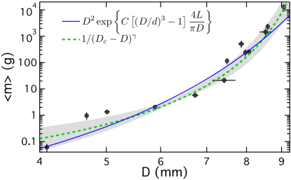
To locate the critical hole size for the nominal clogging transition, we follow standard procedure by fitting the average mass discharged before a clog occurs to a diverging power-law function:
| (1) |
Data and fit are shown respectively as symbols and dashed line in Fig. 1. The fit given an exponent of , consistent with prior observations. And it gives the estimated location of the putative clogging transition as mm. This is an important number, that will be marked in several plots below. The uncertainty in and , indicated by the grey band in Fig. 1 is a consequence of both the error in the variables and varying the fitting range. Equivalently, we may fit the data to a form suggested by Ref. Thomas and Durian (2015):
| (2) |
where g/cm3 is the bulk density of the tapioca. In Ref. Thomas and Durian (2015), we reported , a sampling length , and . Here we fix and find consistent values of and . Fit to this latter form is overlaid as the solid line. The fits for both the exponential and the divergent form are very good: the ratio of for the exponential form to the divergent form is 1.05. We cannot therefore readily distinguish from such fits whether there exists a well-defined clogging transition for this hopper geometry.
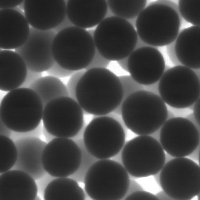
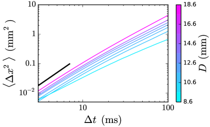
We use a high-speed camera operating at 1 kHz frame rate to acquire images of the back-lit hopper. Only the grains at the wall nearest to the camera are within clear focus (see Fig. 2). The positions of the particles are found to an accuracy of approximately 4 microns. The distance that the particles move between frames is far shorter than the typical distance between grains. We can therefore use the Crocker-Grier method to link the particle trajectories between frames Crocker and Grier (1996). As a demonstration, Fig. 3 shows the mean-squared horizontal displacement versus delay time in a region near the exit. Note that holds at short times. Therefore, the spatial and temporal resolution is good enough to access the expected ballistic regime at short times and we thus have access to the true instantaneous particle speeds.
To find the instantaneous velocity of particle at time , we fit in the range ms ms to a second-order polynomial. Note that here we define , and at the center of the slit. We restricted our data collection largely to a tall, narrow region centered above the slit, with cm and cm.
IV Velocity distributions
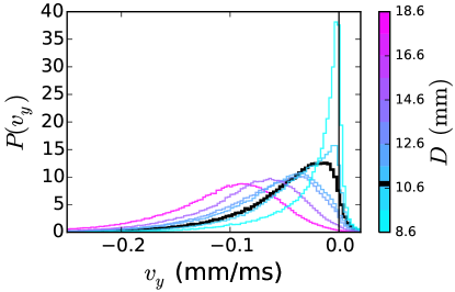
We begin by evaluating the distributions of these particle velocities, which depend sensitively both on the hopper opening size and the location of the grain within the hopper. Example velocity distributions in the vertical -direction for the full range of opening sizes, in a region the the exit, are shown in Fig. 4. The black heavy curve indicates the distribution of when is near the putative clogging transition . These are the velocity distributions for of the individual particles in a given region over all time. They are therefore distinct from the ensemble velocity statistics, discussed in detail in Section V.
IV.1 Average flow
We begin by considering the average of these velocity distributions. We note how previous work has shown that the Beverloo equation for the average flow rate as a function of hole size works perfectly well for flows both above and below the clogging transition. In particular, Fig. 1 of Ref. Thomas and Durian (2013) demonstrates how there is no kink, or discontinuity in the first derivative, of at the putative transition .
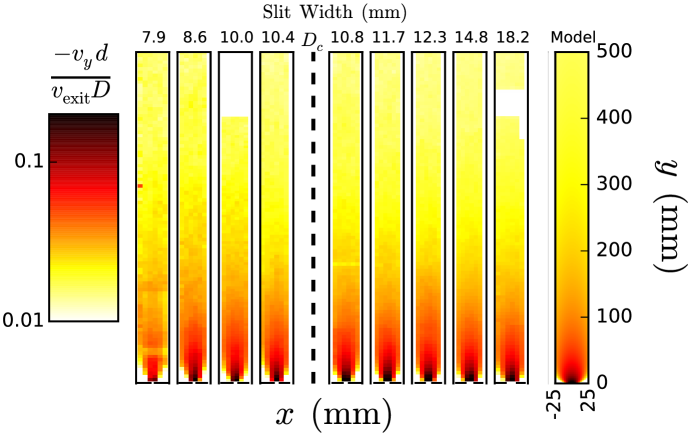
Not only is the discharge rate agnostic about the clogging transition, but the coarse-grained average (or hydrodynamic) granular velocities at various locations within the hopper also do not display any dependence on . Note that we determine the hydrodynamic velocity at by taking both the ensemble and the time average of all grains within the bin at for all time: . The hydrodynamic velocity fields have long been understood to follow the empirical form Nedderman and Tüzün (1979); Tüzün and Nedderman (1979); Samadani et al. (1999); Choi et al. (2005); Garcimartín et al. (2011):
| (3) |
where is a length scale observed to typically range from to .
The hydrodynamic velocity field for our system is shown in Fig. 5 for hoppers with slit widths both smaller and larger than mm. The bins are rectangular regions typically 7 mm 5 mm. As with the average flow rates, the shape is independent of , with no difference of behavior above or below the clogging transition. For comparison with Eq. (3), we plot the expectation when on the far right of Fig. 5.
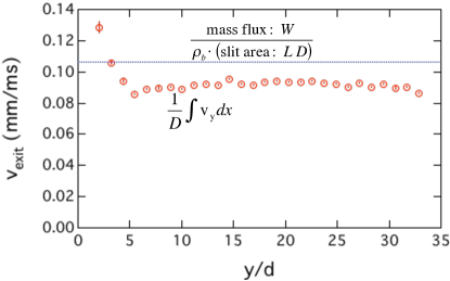
Although we are only imaging the layer of the grains at the wall, we confirm that the behavior here is fairly representative of the flow in the bulk. For this we determine the average speed of the exiting grains for a slit width as:
| (4) |
where is the average mass flow rate, is the bulk density of the tapioca, and is the length of the slit. At the orifice, this may be equivalently found by measuring the velocity directly: . By conservation of mass, we must have, for all :
| (5) |
By comparing the values of found from Eq. (4) and Eq. (5), we may evaluate how the measured flow fields compare with the bulk flow rate. This is shown in Fig. 6. The flow rates imaged at the surface are within about of the flow rate within the bulk. We therefore conclude that friction with the walls does not significantly alter the flow patterns in this hopper.
IV.2 Velocity distribution moments
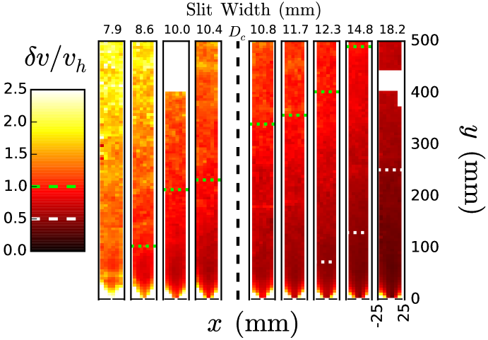
While the average flow behavior clearly does not provide evidence of the clogging transition, we may reasonably ask about the higher-order moments, including the standard deviation and the skewness of the velocity distribution. Is there a significant change at ? Fig. 7 demonstrates clearly that this is not so. Here, we measure from the velocity distributions in both the horizontal and vertical directions: , where is the standard deviation of all the particle velocities within a particular binned region. (This is distinct from measuring the temporal fluctuations in the ensemble average particle velocities.) The associated granular temperature is . Unlike the maps of the hydrodynamic velocity, there is a very significant hole-size dependence in . The fluctuations in the grain velocity are substantially larger for smaller slit widths. This occurs throughout the entire hopper, and is reminiscent of the results obtained in Refs. Menon and Durian (1997); Lemieux and Durian (2000a); Katsuragi et al. (2010) using diffusing-wave spectroscopy. For the smallest slit width, holds everywhere. However, this transition from low fluctuations to high fluctuations is smooth as a function of . There is no signature of a clogging transition in the .
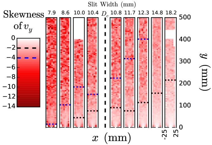
Not only do hoppers more prone to clogging have larger fluctuations relative to the mean, but the fluctuations in the velocity are also more anisotropic. As evidence of this behavior, maps of the skewness in are shown in Fig. 8. Note that the sign of the skewness is always negative, that is, the distributions of the velocities are skewed in the downwards direction. As with the granular temperature, the magnitude of the skewness becomes larger everywhere in the hopper for smaller values of . However, also like all the measures considered, there is no critical change in the skewness upon transitioning through .
V Intermittency
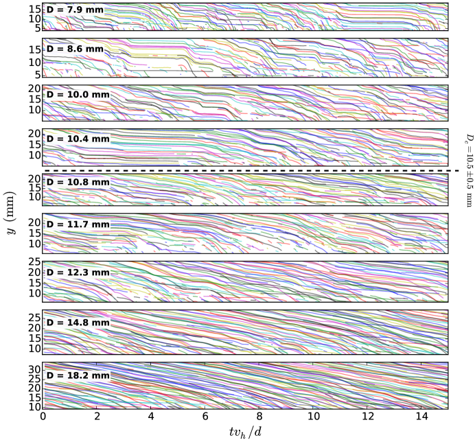
The previous measures of the flow considered only time-averaged statistics of individual particles. However, a very striking feature of slow granular hopper flow is the development of collectively intermittent dynamics as the hole size decreases. In particular, multiple grains in a viewing region speed up and slow down in tandem, more so for smaller holes. This is illustrated in Fig. 9, where we plot vertical particle positions versus time. We do so only for grains in a square viewing region directly near the exit: the bottom of the region is at . The region size is set by as , and the region is centered about . Here, we scale time on the -axis by the typical time that a grain translates by its own diameter. The difference in behavior between small and large is quite striking: for small , many grains often come to a near-stop before the flow resumes again. Clogging would be an extreme instance in which the grains actually stop altogether, forever. For large , there is also significant collective behavior, but the ensemble velocity instead fluctuates between periods of slightly faster and slightly slower flow. Clearly the flow is more intermittent for small than for large . This can also be seen in movies of the flow near the exit for two different hopper sizes sup . Next, we consider several ways to characterize this intermittency.
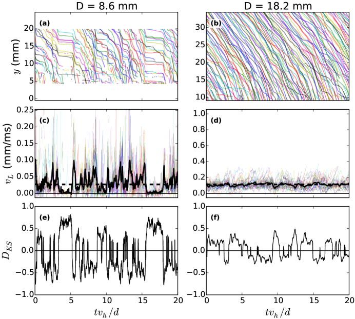
A simple measure to describe the collective behavior of the grains in the region is in terms of the ensemble velocity, , where the average is taken over all particles in a region of interest at time . Here, we consider the component of this ensemble velocity in the direction of the average flow, or the longitudinal velocity: . In Fig. 10c,d, we display both the individual and the ensemble over time for a highly intermittent case (c) and a case with little intermittency (d). Not only is larger, but the relative ensemble velocity fluctuations are larger for smaller .
The ensemble-averaged velocity is helpful for describing the intermittency of the collective behavior, but it does not provide the full story. We wish to understand how the collective behavior as a whole differs from one time to another. For example, heap granular flow exhibits extreme intermittency with characteristic on/off time scales Lemieux and Durian (2000b). We hypothesize that the velocity distributions during the “pause events” seen in Fig. 10a,c are characterized by different velocity distributions than during regular flow.
To test this hypothesis, we calculate the Kolmogorov-Smirnov (K-S) statistic comparing the velocity distribution at time with the distribution over all time Press et al. (2007). The two-sample Kolmogorov-Smirnov (KS) statistic is defined as the maximum distance between the sample cumulative distributions. When its magnitude is near unity, the distributions are very dissimilar. If it is near zero, then the distributions are similar. We add an additional tweak to this measure by determining the signed KS statistic . This is identical to the usual KS statistic described above, except that it is negative when the distribution is greater than the distribution for all the data. The result is shown in Fig. 10e,f, respectively. Contrasting these two, it is clear that more intermittent flow is characterized by a greater heterogeneity of the velocity distributions over time.
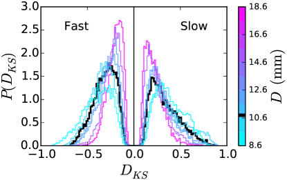
The intermittency as a function of opening size is further illuminated in Fig. 11, which shows the the probability distribution of for various slit widths . When is smaller, the velocity distributions at any given time are more likely to deviate from the long-time velocity distribution, as seen by the larger distribution in the magnitudes of . Note also that for all slits there is a minimum value of : at all times deviates significantly from . We can therefore consider the collective particle behavior at any time to be either “fast” or “slow”, depending on the sign of .
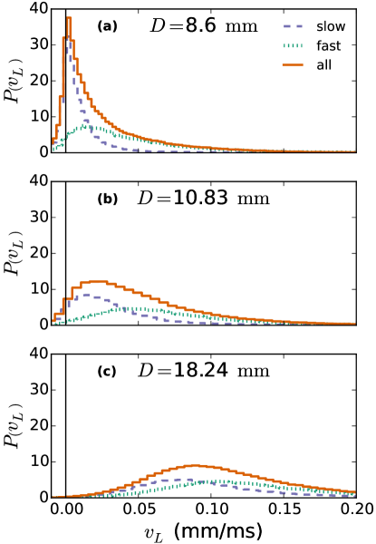
For any slit width, we classify a given particle velocity as “fast” or “slow” if or , respectively. The separate velocity distributions for the particles at fast or slow times are shown in Fig. 12 for several different . When is small, is very different for the fast and the slow cases. As seen in Fig. 10c, the ensemble velocity switches between “flowing” and “paused” states. However, for larger , the distributions are much more similar, and flow typically switches instead between “fast” and “slow” states.
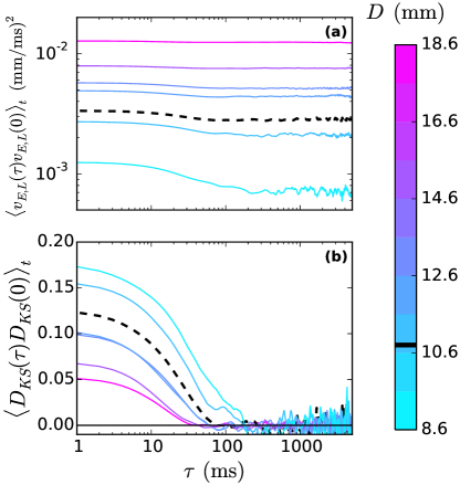
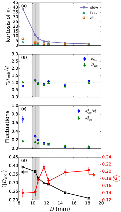
Next, we identify the time scales associated with this intermittency. The temporal autocorrelation functions of and are calculated and displayed in Fig. 13(a) and Fig. 13(b), respectively. We define the time scale of the autocorrelation function as the value of at which the autocorrelation function has fallen of the distance from the value at to the baseline. Dividing by the characteristic time of grain motion at the exit , we see in Fig. 14b that the intermittency time scale is unsurprisingly identical to the time scale of the exiting grain motion. There is no diverging time scale associated with intermittency. In fact, the time scale for intermittency is simply set by the sampling rate of the clogging process.
However, the magnitude of the intermittency, evident in the difference between the -intercept and the baseline of the autocorrelation plots of Fig. 13, does increase for flows more prone to clogging. This is illustrated in Fig. 14(c). However, note that there is no kink in this quantity in the clogging transition. Alternatively, intermittency could be quantified by the absolute value of rather than its standard deviation. This measure has the advantage in that its significance can be readily evaluated, as detailed in Ref. Press et al. (2007). The calculated value is the probability of randomly measuring a value of at least as large as the one observed. The average values of , as well as the average values of the -values, where the averages for both are taken over all time, is shown in Fig. 14(d). As with , grows steadily with decreasing opening size. Additionally, the -values for are greater for smaller as well, indicating that the growth of is not a systematic effect due to smaller number of grains in the sampled region.
Finally, we may also describe intermittency by examining how the velocity distribution of grains during the “slow” events changes with (blue dashed lines in Fig. 12). We do this by calculating the excess kurtosis of these distributions, and plot in Fig. 14(a). The slow velocity distributions deviate substantially from Gaussian as decreases. However, as with the fluctuations, there is no signature of in this behavior.
VI Intermittency and height dependence
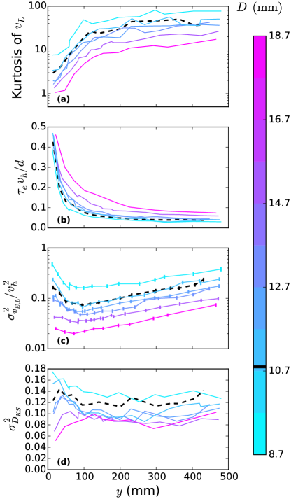
The flow near the hopper exit is more intermittent when it is more prone to clogging. However, the intermittency also varies throughout the hopper. Since width of the flowing region grows with height, the flows ought to be slower/more-intermittent higher up and faster/more-smooth near the exit. Perhaps there is a boundary between intermittent and smooth regions that moves down toward the outlet as the size decreases toward a clogging transition? To investigate, we evaluate large rectangular regions centered about . These are not the same bin sizes as displayed in the heat maps; in order to have sufficient statistics, we require that the average number of sampled configurations be approximately 400. We plot the kurtosis of the longitudinal velocity in Fig. 15(a). Following a similar trend as that shown in Fig. 14, we now see that the non-gaussian character of the velocity distributions grows everywhere in the hopper as . We also evaluate the autocorrelation time scale for at different , and scale the result by . Shown in Fig. 15(b), this demonstrates (in parallel with Fig. 14(b)) that nowhere is there an intermittency time scale longer than the inverse of the local average flow rate. As with the kurtosis of , we find that the relative fluctuations are a monotonic function of the slit width (Fig. 15(c)).
The intermittency measure is displayed in Fig. 15(d). Here, we see clearly that the intermittency grows with the increasing likelihood of clogging. However, the height dependence of is very different than that of . For most hoppers, the flow is most intermittent near the exit, decreases with increasing , and plateaus far from the aperture. This demonstrates that the Kolmogorov-Smirnov statistic is a unique intermittency measurement which provides information not accessible from the instantaneous velocity distributions such as the kurtosis, skewness, or . Furthermore, the change in intermittency with height is not analogous to the change of intermittency with opening size. Both and grow with decreasing . However, they are not monotonic functions of .
VII Conclusion
In conclusion, we have demonstrated that there is no critical change in behavior in granular flow near the putative clogging transition. Relative velocity fluctuations , skewness in velocity, and intermittency magnitude all grow for flows more prone to clogging. However, there is no signature of the clogging transition in the variation any of these measures with hole size. This supports our suggestion in Ref. Thomas and Durian (2015) that there is no well-defined clogging transition, and that is simply a hole size at which the probability for a flow to clog on laboratory time scales disappears.
We have proposed what we believe is a useful new measure for quantifying intermittency and the tendency for flows to fluctuate between different parent velocity distributions. While in this case we simply considered the alternation between fast and slow flows, this method can easily be generalized to encompass more complicated cases.
Finally, we find no evidence of a distinct intermittency time scale anywhere in the hopper, either in the ensemble average flow rate or the intermittency . The time scales for both of these quantities to is identical. For both, the longest time scale anywhere in a hopper of a given hole size is , the rate at which grains move by their own diameter in the exit region. Significantly, there is no evidence of a diverging time scale, either as or . Hoppers with smaller hole sizes are not closer to jamming. Rather, hoppers with smaller hole sizes are more likely to fall into a jammed state due to the smaller number of grains at the exit that are required to be “pre-clogged”.
We previously demonstrated that clogging is a Poisson sampling process independent over times greater . Together with the lack of a long time-scale for intermittency, this means that one cannot predict a clog with advance notice greater than by investigating the system dynamics. However, these results are for flows whose intermittency is set by the sampling behavior at the exit. It would be instructive to expand this analysis to cases with other sources of intermittency, for example, where interaction between the grains and the interstitial fluid contribute to intermittency. Do these other cases of intermittency coupling provide the necessary memory in the system to break the Poissonian nature of the sampling? Such explorations will further our general understanding of intermittent phenomena in systems near jamming in general and near clogging in particular.
Acknowledgements.
This work was supported by the National Science Foundation through Grant No. DMR-1305199.References
- Duran (2000) J. Duran, Sands, powders, and grains: An introduction to the physics of granular materials (Springer, NY, 2000).
- Franklin and Shattuck (2016) S. V. Franklin and M. D. Shattuck, Handbook of Granular Materials (CRC Press, NY, 2016).
- Nedderman and Tüzün (1979) R. M. Nedderman and U. Tüzün, Powder Technol. 22, 243 (1979).
- Tüzün and Nedderman (1979) U. Tüzün and R. M. Nedderman, Powder Technol. 24, 257 (1979).
- Samadani et al. (1999) A. Samadani, A. Pradhan, and A. Kudrolli, Phys. Rev. E 60, 7203 (1999).
- Choi et al. (2005) J. Choi, A. Kudrolli, and M. Z. Bazant, Journal of Physics: Condensed Matter 17 (2005).
- Garcimartín et al. (2011) A. Garcimartín, I. Zuriguel, A. Janda, and D. Maza, Phys. Rev. E 84, 031309 (2011).
- Beverloo et al. (1961) W. A. Beverloo, H. A. Leniger, and J. van de Velde, Chem. Eng. Sci. 15, 260 (1961).
- Nedderman et al. (1982) R. M. Nedderman, U. Tuzun, S. B. Savage, and G. T. Houlsby, Chem. Eng. Sci. 37, 1597 (1982).
- Mankoc et al. (2007) C. Mankoc, A. Janda, R. Arévalo, J. M. Pastor, I. Zuriguel, A. Garcimartín, and D. Maza, Granular Matter 9, 407 (2007).
- Aguirre et al. (2010) M. A. Aguirre, J. G. Grande, A. Calvo, L. A. Pugnaloni, and J.-C. Géminard, Phys. Rev. Lett. 104, 238002 (2010).
- Hilton and Cleary (2011) J. E. Hilton and P. W. Cleary, Phys. Rev. E 84, 011307 (2011).
- Janda et al. (2012) A. Janda, I. Zuriguel, and D. Maza, Phys. Rev. Lett. 108, 248001 (2012).
- Rubio-Largo et al. (2015) S. M. Rubio-Largo, A. Janda, D. Maza, I. Zuriguel, and R. C. Hidalgo, Phys. Rev. Lett. 114, 238002 (2015).
- Dunatunga and Kamrin (2015) S. Dunatunga and K. Kamrin, J. Fluid Mech. 779, 483 (2015).
- Manna and Herrmann (2000) S. S. Manna and H. J. Herrmann, Eur. Phys. J. E 1, 341 (2000).
- To et al. (2001) K. To, P. Y. Lai, and H. K. Pak, Phys. Rev. Lett. 86, 71 (2001).
- Zuriguel et al. (2005) I. Zuriguel, A. Garcimartín, D. Maza, L. A. Pugnaloni, and J. M. Pastor, Phys. Rev. E 71, 051303 (2005).
- Janda et al. (2008) A. Janda, I. Zuriguel, A. Garcimartín, L. A. Pugnaloni, and D. Maza, Europhys. Lett. 84, 44002 (2008).
- Mankoc et al. (2009) C. Mankoc, A. Garcimartín, I. Zuriguel, D. Maza, and L. A. Pugnaloni, Phys. Rev. E 80, 011309 (2009).
- Sheldon and Durian (2010) H. G. Sheldon and D. J. Durian, Granular Matter 12, 579 (2010).
- Thomas and Durian (2013) C. C. Thomas and D. J. Durian, Phys. Rev. E 87, 052201 (2013).
- Zuriguel (2014) I. Zuriguel, Papers in Physics 6, 060014 (2014).
- Thomas and Durian (2015) C. C. Thomas and D. J. Durian, Phys. Rev. Lett. 114, 178001 (2015).
- Menon and Durian (1997) N. Menon and D. J. Durian, Science 275, 1920 (1997).
- Lemieux and Durian (2000a) P. Lemieux and D. Durian, Phys. Rev. Lett. 85, 4273 (2000a).
- Katsuragi et al. (2010) H. Katsuragi, A. R. Abate, and D. J. Durian, Soft Matter 6, 3023 (2010).
- Berthier et al. (2011) L. Berthier, G. Biroli, J.-P. Bouchaud, L. Cipelletti, and W. van Saarloos, eds., Dynamical Heterogeneities in Glasses, Colloids, and Granular Media (Oxford University Press, NY, 2011).
- Tewari et al. (2013) S. Tewari, M. Dichter, and B. Chakraborty, Soft Matter 9, 5016 (2013).
- Mersch et al. (2010) E. Mersch, G. Lumay, F. Boschini, and N. Vandewalle, Phys. Rev. E 81, 041309 (2010).
- Wu et al. (1993) X.-l. Wu, K. J. Måløy, A. Hansen, M. Ammi, and D. Bideau, Phys. Rev. Lett. 71, 1363 (1993).
- Bertho et al. (2003) Y. Bertho, F. Giorgiutti-Dauphiné, and J.-P. Hulin, Phys. Fluids 15, 3358 (2003).
- Börzsönyi and Kovács (2011) T. Börzsönyi and Z. Kovács, Phys. Rev. E 83, 032301 (2011).
- Uñac et al. (2012) R. O. Uñac, A. M. Vidales, and L. A. Pugnaloni, J. Stat. Mech. - Theory and Expt. 2012, 04008 (2012).
- Janda et al. (2009) A. Janda, R. Harich, I. Zuriguel, D. Maza, P. Cixous, and A. Garcimartín, Phys. Rev. E 79, 031302 (2009).
- Vivanco et al. (2012) F. Vivanco, S. Rica, and F. Melo, Granular Matter 14, 563 (2012).
- Saraf and Franklin (2011) S. Saraf and S. V. Franklin, Phys. Rev. E 83, 030301 (2011).
- Crocker and Grier (1996) J. C. Crocker and D. G. Grier, J. Colloid Interface Sci. 179, 298 (1996).
- (39) See Supplemental Material at … for a video illustrating intermittent flow for a small hole ( mm, left) and smooth flow for a large hole ( mm, right). For comparison, the nominal clogging transition is at mm. Time is scaled by the hydrodynamic speed in the viewing window, so that both have the same average viewed time for grains to fall a distance of one grain diameter.
- Lemieux and Durian (2000b) P. Lemieux and D. J. Durian, Applied Optics 40, 3984 (2000b).
- Press et al. (2007) W. H. Press, S. A. Teukolsky, W. T. Vetterling, and B. P. Flannery, Numerical Recipes: The Art of Scientific Computing (Cambridge University Press, 2007).