Concurrent Data Structures Linked in Time

Abstract

Arguments about correctness of a concurrent data structure are typically carried out by using the notion of linearizability and specifying the linearization points of the data structure’s procedures. Such arguments are often cumbersome as the linearization points’ position in time can be dynamic (depend on the interference, run-time values and events from the past, or even future), non-local (appear in procedures other than the one considered), and whose position in the execution trace may only be determined after the considered procedure has already terminated.

In this paper we propose a new method, based on a separation-style logic, for reasoning about concurrent objects with such linearization points. We embrace the dynamic nature of linearization points, and encode it as part of the data structure’s auxiliary state, so that it can be dynamically modified in place by auxiliary code, as needed when some appropriate run-time event occurs. We name the idea linking-in-time, because it reduces temporal reasoning to spatial reasoning. For example, modifying a temporal position of a linearization point can be modeled similarly to a pointer update in separation logic. Furthermore, the auxiliary state provides a convenient way to concisely express the properties essential for reasoning about clients of such concurrent objects. We illustrate the method by verifying (mechanically in Coq) an intricate optimal snapshot algorithm due to Jayanti, as well as some clients.

1 Introduction

Formal verification of concurrent objects commonly requires reasoning about linearizability [19]. This is a standard correctness criterion whereby a concurrent execution of an object’s procedures is proved equivalent, via a simulation argument, to some sequential execution. The clients of the object can be verified under the sequentiality assumption, rather than by inlining the procedures and considering their interleavings. Linearizability is often established by describing the linearization points (LP) of the object, which are points in time where procedures take place, logically. In other words, even if the procedure physically executes across a time interval, exhibiting its linearization point enables one to pretend, for reasoning purposes, that it occurred instantaneously (i.e., atomically); hence, an interleaved execution of a number of procedures can be reduced to a sequence of atomic events.

Reasoning about linearization points can be tricky. Many times, a linearization point of a procedure is not local, but may appear in another procedure or thread. Equally bad, linearization points’ place in time may not be determined statically, but may vary based on the past, and even future, run-time information, thus complicating the simulation arguments. A particularly troublesome case is when run-time information influences the logical order of a procedure that has already terminated. This paper presents a novel approach to specification of concurrent objects, in which the dynamic and non-local aspects inherent to linearizability can be represented in a procedure-local and thread-local manner.

The starting point of our idea is to realize what are the shortcomings of linearizability as a canonical specification method for concurrent objects. Consider, for instance, the following two-threaded program manipulating a correct implementation of stack by invoking its push and pop methods, which are atomic, i.e., linearizable:

push(3);	push(4)
t1 := pop();	t2 := pop();

Assuming that the execution started in an empty stack, we would like to derive that it returns an empty stack and (t1, t2) is either (3, 4) or (4, 3). Linearizability of the stack guarantees that the overall trace of push/pop calls is coherent with respect to a sequential stack execution. However, it does not capture client-specific partial knowledge about the ordering of particular push/pop invocations in sub-threads, which is what allows one to prove the desired result as a composition of separately-derived partial specifications of the left and the right thread.

This thread-local information, necessary for compositional reasoning about clients, can be captured in a form of auxiliary state [33] (a generalization of history variables [2]), widely used in Hoare-style specifications of concurrent objects [37, 27, 24, 23]. A testament of expressivity of Hoare-style logics for concurrency with rich auxiliary state are the recent results in verification of fine-grained data structures with helping [37], concurrent graph manipulations [36], barriers [23, 10], and even non-linearizable concurrent objects [38].

Although designed to capture information about events that happened concurrently in the past (hence the original name history variables), auxiliary state is known to be of little use for reasoning about data structures with speculative executions, in which the ordering of past events may depend on other events happening in the future. Handling such data structures requires specialized metatheory [28] that does not provide convenient abstractions such as auxiliary state for client-side proofs. This is one reason why the most expressive client-oriented concurrency logics to date avoid reasoning about speculative data structures altogether [23].

Our contributions

The surprising result we present in this paper is that by allowing certain internal (i.e., not observable by clients) manipulations with the auxiliary state, we can use an existing program logic for concurrency, like, e.g., FCSL [31, 36], to specify and verify algorithms whose linearizability argument requires speculations, i.e., depends on the dynamic reordering of events based on run-time information from the future. To showcase this idea, we provide a new specification (spec) and the first formal proof of a very sophisticated snapshot algorithm due to Jayanti [22], whose linearizability proof exhibits precisely such kind of dependence.

While we specify Jayanti’s algorithm by means of a separation-style logic, the spec nevertheless achieves the same general goals as linearizability, combined with the benefits of compositional Hoare-style reasoning. In particular, our Hoare triple specs expose the logical atomicity of Jayanti’s methods (Section 3), while hiding their true fine-grained and physically non-atomic nature. The approach also enables that the separation logic reasoning is naturally applied to clients (Section 4). Similarly to linearizability, our clients can reason out of procedures’ spec, not code. We can also ascribe the same spec to different snapshot algorithms, without modifying client’s code or proof.

In more detail, our approach works as follows. We use shared auxiliary state to record, as a list of timed events (e.g., writes occurring at a given time), the logical order in which the object’s procedures are perceived to execute, each instantaneously (Section 5). Tracking this time-related information through state enables us to specify its dynamic aspects. We can use auxiliary code to mutate the logical order in place, thereby permuting the logical sequencing of the procedures, as may be needed when some run-time event occurs (Sections 6 and 7). This mutation is similar to updating pointers to reorder a linked list, except that it is executed over auxiliary state storing time-related data, rather than over real state. This is why we refer to the idea as linking-in-time.

Encoding temporal information by way of representing it as mutable state allows us to use FCSL off-the-shelf to verify example programs. In particular, FCSL has been implemented in the proof assistant Coq, and we have fully mechanized the proof of Jayanti’s algorithm [1].

$$\begin{array}[]{rl}{\text{{\scriptsize{1}}}\nobreak\leavevmode}&\text{{\small{write}}}\ (p,\,v)\ \{\\ {\text{{\scriptsize{2}}}\nobreak\leavevmode}&\leavevmode\nobreak\ \leavevmode\nobreak\ \leavevmode\nobreak\ {p}\,{:=}\,{v};\\ {\text{{\scriptsize{3}}}\nobreak\leavevmode}&\leavevmode\nobreak\ \leavevmode\nobreak\ \leavevmode\nobreak\ b\leftarrow\textsf{\small{read}}(S);\\ {\text{{\scriptsize{4}}}\nobreak\leavevmode}&\leavevmode\nobreak\ \leavevmode\nobreak\ \leavevmode\nobreak\ \text{{if}}\ b\\ {\text{{\scriptsize{5}}}\nobreak\leavevmode}&\leavevmode\nobreak\ \leavevmode\nobreak\ \leavevmode\nobreak\ \text{{then}}\ {(\text{{\small{fwd}}}\leavevmode\nobreak\ p)}\,{:=}\,{v}\}\\ &\\ &\\ &\text{{\small{fwd}}}\ (p:\text{{\small{ptr}}})\ \{\\ &\leavevmode\nobreak\ \leavevmode\nobreak\ \leavevmode\nobreak\ \text{{return}}\ (p=x)\ \text{{\small{?}}}\ \mathit{fx}\text{{\small{:}}}\ \mathit{fy}\ \}\end{array}$$

$$\begin{array}[]{rl}{\text{{\scriptsize{6}}}\nobreak\leavevmode}&\text{{\small{scan}}}\ :\ (A\times A)\ \{\\ {\text{{\scriptsize{7}}}\nobreak\leavevmode}&\leavevmode\nobreak\ \leavevmode\nobreak\ \leavevmode\nobreak\ \leavevmode\nobreak\ {S}\,{:=}\,{\text{{\small{true}}}};\\ {\text{{\scriptsize{8}}}\nobreak\leavevmode}&\leavevmode\nobreak\ \leavevmode\nobreak\ \leavevmode\nobreak\ \leavevmode\nobreak\ {\mathit{fx}}\,{:=}\,{\bot};\\ {\text{{\scriptsize{9}}}\nobreak\leavevmode}&\leavevmode\nobreak\ \leavevmode\nobreak\ \leavevmode\nobreak\ \leavevmode\nobreak\ {\mathit{fy}}\,{:=}\,{\bot};\\ {\text{{\scriptsize{10}}}\nobreak\leavevmode}&\leavevmode\nobreak\ \leavevmode\nobreak\ \leavevmode\nobreak\ \leavevmode\nobreak\ \mathit{vx}\leftarrow\textsf{\small{read}}(x);\\ {\text{{\scriptsize{11}}}\nobreak\leavevmode}&\leavevmode\nobreak\ \leavevmode\nobreak\ \leavevmode\nobreak\ \leavevmode\nobreak\ \mathit{vy}\leftarrow\textsf{\small{read}}(y);\\ {\text{{\scriptsize{12}}}\nobreak\leavevmode}&\leavevmode\nobreak\ \leavevmode\nobreak\ \leavevmode\nobreak\ \leavevmode\nobreak\ {S}\,{:=}\,{\text{{\small{false}}}};\\ {\text{{\scriptsize{13}}}\nobreak\leavevmode}&\leavevmode\nobreak\ \leavevmode\nobreak\ \leavevmode\nobreak\ \leavevmode\nobreak\ \mathit{ox}\leftarrow\textsf{\small{read}}(\mathit{fx});\\ {\text{{\scriptsize{14}}}\nobreak\leavevmode}&\leavevmode\nobreak\ \leavevmode\nobreak\ \leavevmode\nobreak\ \leavevmode\nobreak\ \mathit{oy}\leftarrow\textsf{\small{read}}(\mathit{fy});\\ {\text{{\scriptsize{15}}}\nobreak\leavevmode}&\leavevmode\nobreak\ \leavevmode\nobreak\ \leavevmode\nobreak\ \leavevmode\nobreak\ \mathit{rx}\leftarrow\text{{if}}\ (\mathit{ox}\neq\bot)\ \text{{then}}\ \mathit{ox}\ \text{{else}}\ \mathit{vx};\\ {\text{{\scriptsize{16}}}\nobreak\leavevmode}&\leavevmode\nobreak\ \leavevmode\nobreak\ \leavevmode\nobreak\ \leavevmode\nobreak\ \mathit{ry}\leftarrow\text{{if}}\ (\mathit{oy}\neq\bot)\ \text{{then}}\ \mathit{oy}\ \text{{else}}\ \mathit{vy};\\ {\text{{\scriptsize{17}}}\nobreak\leavevmode}&\leavevmode\nobreak\ \leavevmode\nobreak\ \leavevmode\nobreak\ \leavevmode\nobreak\ \text{{return}}\leavevmode\nobreak\ (\mathit{rx},\mathit{ry})\}\\ \end{array}$$

Figure 1: Jayanti’s single-scanner/single-writer snapshot algorithm.

2 Verification challenge and main ideas

Jayanti’s snapshot algorithm [22] provides the functionality of a shared array of size $m$, operated on by two procedures: write, which stores a given value into an element, and scan, which returns the array’s contents. We use the single-writer/single-scanner version of the algorithm. which assumes that at most one thread writes into an element, and at most one thread invokes the scanner, at any given time. In other words, there is a scanner lock and $m$ per-element locks. A thread that wants to scan, has to acquire the scanner lock first, and a thread that wants to write into element $i$ has to acquire the $i$-th element lock. However, scanning and writing into different elements can proceed concurrently. This is the simplest of Jayanti’s algorithms, but it already exhibits linearization points of dynamic nature. We also restrict the array size to $m\,{=}\,2$ (i.e., we consider two pointers $x$ and $y$, instead of an array). This removes some tedium from verification, but exhibits the same conceptual challenges.

The difficulty in this snapshot algorithm is ensuring that the scanner returns the most recent snapshot of the memory. A naïve scanner, which simply reads $x$ and $y$ in succession, is unsound. To see why, consider the following scenario, starting with $x=5$, $y=0$. The scanner reads $x$, but before it reads $y$, another thread preempts it, and changes $x$ to $2$ and, subsequently, $y$ to $1$. The scanner continues to read $y$, and returns $x=5,y=1$, which was never the contents of the memory. Moreover, $(x,y)$, changed from $(5,0)$ to $(2,0)$ to $(2,1)$ as a result of distinct non-overlapping writes; thus, it is impossible to find a linearization point for the scan because linearizability only permits reordering of overlapping operations.

To ensure a sound snapshot, Jayanti’s algorithm internally keeps additional forwarding pointers $\mathit{fx}$ and $\mathit{fy}$, and a boolean scanner bit $S$. The implementation is given in Figure 1. The intuition is as follows. A writer storing $v$ into $p$ (line 2), will additionally store $v$ into the forwarding pointer for $p$ (line 5), provided $S$ is set. If the scanner missed the write and instead read the old value of $p$ (lines 10–11), it will have a chance to catch $v$ via the forwarding pointer (lines 13–14). The scanner bit $S$ is used by writers (line 3) to detect a scan in progress, and forward $v$.

l: write (x,2);	c: scan ()	r: write (x,3)
write (y,1)

(a) Parallel composition of three threads l, c, r.

1 c: S := true 2 c: fx := $\bot$ 3 c: fy := $\bot$ 4 c: read(x) // vx <- 5 5 c: read(y) // vy <- 0 6 l: x := 2 7 l: read(S) // b <- true 8 l: fx := 2 9 l: return () 10 r: x := 3

11 l: y := 1 12 l: read(S) // b <- true 13 l: fy := 1 14 l: return () 15 c: S := false 16 r: read(S) // b <- false 17 r: return () 18 c: read(fx) // ox <- 2 19 c: read(fy) // oy <- 1 20 c: return (2,1)

(b) A possible interleaving of the threads in (2(a)).

Figure 2: An example leading to a scanner miss.

As Jayanti proves, this implementation is linearizable. Informally, every overlapping calls to write and scan can be rearranged to appear as if they occurred sequentially. To illustrate, consider the program in Figure 2(a), and one possible interleaving of its primitive memory operations in Figure 2(b). The threads l, c, and r, start with $x=5,y=0$. The thread c is scheduled first, and through lines 1–5 sets the scanner bit, clears the forwarding pointers, and reads $x=5,y=0$. Then l intervenes, and in lines 6–9, overwrites $x$ with $2$, and seeing $S$ set, forwards $2$ to $\mathit{fx}$. Next, r and l overlap, writing $3$ into $x$ and $1$ into $y$. However, while $1$ gets forwarded to $\mathit{fy}$ (line 13), $3$ is not forwarded to $\mathit{fx}$, because $S$ was turned off in line 15 (i.e., the scan is no longer in progress). Hence, when c reads the forwarded values (lines 18, 19), it returns $x=2,y=1$.

While $x\,{=}\,2,y\,{=}\,1$ was never the contents of the memory, returning this snapshot is nevertheless justified because we can pretend that the scanner missed r’s write of $3$. Specifically, the events in Figure 2(b) can be reordered to represent the following sequential execution:

$$\hfill\mathtt{write\,(x,2);\ write\,(y,1);\ scan\,();\ write\,(x,3)}\hfill$$ (1)

Importantly, the client programs have no means to discover that a different scheduling actually took place in real time, because they can access the internal state of the algorithm only via interface methods, write and scan.

This kind of temporal reordering is the most characteristic aspect of linearizability proofs, which typically describe the reordering by listing the linearization points of each procedure. At a linearization point, the procedure’s operations can be spliced into the execution history as an uninterrupted chunk. For example, in Jayanti’s proof, the linearization point of scan is at line 12 in Figure 1, where the scanner bit is unset. The linearization point of write, however, may vary. If write starts before an overlapping scan’s line 12, and moreover, the scan misses the write—note the dynamic and future-dependent nature of this property—, then write should appear after scan; that is, the write’s linearization point is right after scan’s linearization point at line 12. Otherwise, write’s linearization point is at line 2. In the former case, write exactly has a non-local and future-dependent linearization point, because the decision on the logical order of this write depends on the execution of scan in a different thread. This decision takes effect on lines 13–14, which can take place after the execution of write has terminated. For instance, in Figure 2(b) the execution of write in r terminates at step 17, yet, in Jayanti’s proof, the decision to linearize this write after the overlapping scan is taken at line 18, when the scan reads the value from the previous write.

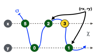
(a)

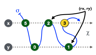
(b)

Figure 3: Changing the logical ordering (solid line $\sigma$) of write events from (5, 0, 2, 3, 1) in (3(a)) to (5, 0, 2, 1, 3) in (3(b)), to reconcile with scan returning the snapshot $x=2,y=1$, upon missing the write of $3$. Dashed lines $\chi$ represent real-time ordering.

Obviously, the high-level pattern of the proof requires tracking the logical ordering of the write and scan events, which differs from their real-time ordering. As the logical ordering is inherently dynamic, depending on properties such as scan missing a write, we formalize it in Hoare logic, by keeping it as a list of events in auxiliary state that can be dynamically reordered as needed. For example, Figure 3 shows the situation in the execution of scan that we reviewed above. We start with the (initializing) writes of $5$ and $0$ already executed, and our program performs the writes of $2$, $3$ and $1$ in the real time order shown by the position of the events on the dashed lines. In Figure 3(a), the logical order $\sigma$ coincides with real-time order, but is unsound for the snapshot $x=2,y=1$ that scan wants to return. In that case, the auxiliary code with which we annotate scan, will change the sequence $\sigma$ in-place, as shown in Figure 3(b).

Our specification and verification challenge then lies in reconciling the following requirements. First, we have to posit specs that say that write performs a write, and scan performs a scan of the memory, with the operations executing in a single logical moment. Second, we need to implement the event reordering discipline so that a method call only reorders events that overlap with it; the logical order of the past events should be preserved. This will be accomplished by introducing yet further structures into the auxiliary state and code. Finally, the specs must hide the specifics of the reordering discipline, which should be internal to the snapshot object. Different snapshot implementations should be free to implement different reorderings, without changing the method specs.

3 Specification

General considerations.

For the purposes of specification and proof, we record a history of the snapshot object as a set of entries of the form $t\mapsto(p,v)$. The entry says that at time $t$ (a natural number), the value $v$ was written into the pointer $p$. We thus identify a write event with a single moment in time $t$, enabling the specs of write and scan to present the view that write events are logically atomic. Moreover, in the case of snapshots, we can ignore the scan events in the histories. The latter do not modify the state in a way observable by clients who can access the shared pointers only via interface methods write and scan.

We keep three auxiliary history variables. The history variables $\chi_{\,\mathsf{s}}$ and $\chi_{\,\mathsf{o}}$ are local to the specified thread, and record the terminated write events carried out by the specified thread, and that thread’s interfering environment, respectively. We refer to $\chi_{\,\mathsf{s}}$ as the self-history, and to $\chi_{\,\mathsf{o}}$ as the other-history [27, 31, 30, 37]. The role of $\chi_{\,\mathsf{o}}$ is to enable the spec of write to situate the performed write event within the larger context of past and ongoing writes, and the spec of scan to describe how it logically reordered the writes that overlapped with it. The third history variable $\chi_{\,\mathsf{j}}$ records the set of write events that are in progress. These are events that have been initiated, timestamped, and have executed their physical write to memory, but have not terminated yet. It is an important component of our auxiliary state design that when a write event terminates, it is moved from $\chi_{\,\mathsf{j}}$ to the invoking thread’s $\chi_{\,\mathsf{s}}$, to indicate the ownership of the write by the invoking thread. We name by $\chi$ the union $\chi_{\,\mathsf{s}}\mathbin{\mathaccent 0{\cdot}\cup}\chi_{\,\mathsf{o}}\mathbin{\mathaccent 0{\cdot}\cup}\chi_{\,\mathsf{j}}$, which is the global history of the data structure. As common in separation logic, the union is disjoint, i.e., it is undefined if the components contain duplicate timestamps. By the semantics of our specs, $\chi$ is always defined, thus $\chi_{\,\mathsf{s}}$, $\chi_{\,\mathsf{o}}$ and $\chi_{\,\mathsf{j}}$ never duplicate timestamps.

The real-time ordering of the timestamped events is the natural numbers ordering on the timestamps. To track the logical ordering, we need further auxiliary notions. The first is the auxiliary variable $\sigma$, whose type is a mathematical sequence. The sequence $\sigma$ is a permutation of timestamps from $\chi$ showing the logical ordering of the events in $\chi$. We write $t_{1}\mathrel{\leq_{\sigma}}t_{2}$, and say that $t_{1}$ is logically ordered before $t_{2}$, if $t_{1}$ appears before $t_{2}$ in $\sigma$. The sequence $\sigma$ resides in joint state, and can be dynamically modified by any thread. For example, the execution of the scanner may reorder $\sigma$, as shown in Figure 3(b). Because $\sigma$ is a sequence, the order $\mathrel{\leq_{\sigma}}$ is linear.

Because sequence $\sigma$ changes dynamically under interference, it is not appropriate for specifications. Thus, our second auxiliary notion is the partial order $\Omega$, a suborder of $\mathrel{\leq_{\sigma}}$ that is stable in the following sense. It relates the timestamps of events whose logical order has been determined, and will not change in the future. Thus $\Omega$ can grow over time, to add new relations between previously unrelated timestamps, but cannot change the old relations.

To illustrate the distinction between the two orders, we refer to Figure 3(a). There, $\sigma$ represents the linear order $5{-}0{-}2{-}3{-}1$, which changes in Figure 3(b) to $5{-}0{-}2{-}1{-}3$. Since $1$ and $3$ exchange places, the stable order $\Omega$ cannot initially relate the two. Thus, in Figure 3(a), $\Omega$ is represented by the Hasse diagram $5{-}0{-}2{<}\!\begin{array}[c]{c}1\\ 3\end{array}$. In Figure 3(b), the relation $1{-}3$ is added to this partial order, making it the linear order $5{-}0{-}2{-}1{-}3$. Note how the previous relations remain unchanged.

The third auxiliary notion is the set $\mathsf{scanned}\,\Omega$ of timestamps. A write’s timestamp is placed in $\mathsf{scanned}\,\Omega$, if that write has been observed by some scanner; that is, the written value is returned in some snapshot, or has been rewritten by another value that is returned in some snapshot. To illustrate, in the above example, $\{5,0,2\}\subseteq\mathsf{scanned}\,\Omega$. Intuitively, we want to model that after a write has been observed, the ordering of the events logically preceding the write must be stabilized, and moreover, must be a sequence. Thus, $\mathsf{scanned}\,\Omega$ is a linearly ordered subset of $\Omega$. The set $\mathsf{scanned}\,\Omega$ can also be seen as representing all the scans that have already been executed. Such representation of scans allows us to avoid tracking scan events directly in the history.

In the sequel, we concretize $\Omega$ and $\mathsf{scanned}\,\Omega$ in terms of $\sigma$ and other auxiliary state. However, we keep the notions abstract in the method specs and in client reasoning. This enables the use of different snapshot algorithms, with the same specs, without invalidating the client proofs. We also mention that $\sigma$, $\Omega$ and $\mathsf{scanned}\,\Omega$ can be encoded as user-level concepts in FCSL, and require no new logic to be developed.

Snapshot specification.

$$\begin{array}[]{l}\mathtt{write}\ (p,v):\begin{array}[t]{l}{{\color[rgb]{0,0,1}\{\chi_{\,\mathsf{s}}=\emptyset\}}}\ {\color[rgb]{0,0,1}\{\exists t\mathord{.}\,\chi_{\,\mathsf{s}}^{\prime}=t\mapsto(p,v)\wedge\mathsf{dom}(\chi_{\,\mathsf{o}})\cup\mathsf{scanned}\,\,\Omega\subseteq\Omega^{\prime}\,{\mathrel{\rotatebox[origin={c}]{270.0}{$\twoheadrightarrow$}}}\,t\}}@C\end{array}\\[5.0pt] \mathtt{scan}:{{\color[rgb]{0,0,1}\{\chi_{\,\mathsf{s}}=\emptyset\}}}\ \!\!\begin{array}[t]{l}{\color[rgb]{0,0,1}\{r\mathord{.}\,\exists t\mathord{.}\,\chi_{\,\mathsf{s}}^{\prime}=\emptyset\!\wedge\!r=\!\mathsf{eval}\ t\,{\Omega^{\prime}}\,{\chi^{\prime}}\wedge\!\mathsf{dom}(\chi)\!\subseteq\Omega^{\prime}\,{\downarrow}\,t\!\wedge\!t\in\mathsf{scanned}\,\Omega^{\prime}\}}@C\end{array}\end{array}$$

Figure 4: Snapshot method specification.

Figure 4 presents our specs for scan and write. These are partial correctness specs that describe how the methods change the state from the precondition (first braces) to the postcondition (second braces), possibly influencing the value $r$ that the procedure returns. We use VDM-style notation with unprimed variables for the state before, and primed variables for the state after the method executes. We use Greek letters for state-dependent values that can be mutated by the method, and Latin letters for immutable variables. The component $C$ is a state transition system (STS) that describes the state space of the algorithm, i.e, the invariants on the auxiliary and real state, and the transitions, i.e., the allowed atomic mutations of the state. For now, we keep $C$ abstract, but will define it in Sections 5 and 6. We denote by $\Omega\,{\downarrow}\,t$ the downward-closed set of timestamps $\Omega\,{\downarrow}\,t=\{s\mid s\ {\Omega}\ t\}$. Let $\Omega\,{\mathrel{\rotatebox[origin={c}]{270.0}{$\twoheadrightarrow$}}}\,t=(\Omega\,{\downarrow}\,t)\setminus\{t\}$.

The spec for write says the following. The precondition starts with the empty self history $\chi_{\,\mathsf{s}}$, indicating that the procedure has not made any writes. In the postcondition, a new write event $t\mapsto(p,v)$ has been placed into $\chi_{\,\mathsf{s}}^{\prime}$. Thus, a call to write wrote $v$ into pointer $p$. The timestamp $t$ is fresh, because $\chi^{\prime}$ does not contain duplicate timestamps. Moreover, the write appears as if it occurred atomically at time $t$, thus capturing the logical atomicity of write.

The next conjunct, $\mathsf{dom}(\chi_{\,\mathsf{o}})\cup\mathsf{scanned}\,\Omega\subseteq\Omega^{\prime}\,{\mathrel{\rotatebox[origin={c}]{270.0}{$\twoheadrightarrow$}}}\,t$, positions the write $t$ into the context of other events. In particular, if $s\in\mathsf{dom}(\chi_{\,\mathsf{o}})$, i.e., if $s$ finished prior to invoking write, then $s$ is logically ordered strictly before $t$. In other words, write cannot reorder prior events that did not overlap with it. The definition of linearizability contains a similar prohibition on reordering non-overlapping events, but here, we capture it using a Hoare-style spec. For similar reasons, we require that $\mathsf{scanned}\,\Omega\subseteq\Omega^{\prime}\,{\mathrel{\rotatebox[origin={c}]{270.0}{$\twoheadrightarrow$}}}\,t$. As mentioned before, $\mathsf{scanned}\,\Omega$ represents all the scans that finished prior to the call to write. Consequently, they do not overlap with write in real time, and have to be logically ordered before $t$.

Notice what the spec of write does not prevent. It is possible that some event, say with a timestamp $s$, finishes in real time before the call of write at time $t$. Events $s$ and $t$ do not overlap, and hence cannot be reordered; thus $s\ {\Omega}\ t$ always. However, the relationship of $s$ with other events that ran concurrently with $s$, may be fixed only later, thus supporting implementation of “future-dependent” nature, such as Jayanti’s.

In the case of scan, we start and terminate with an empty $\chi_{\,\mathsf{s}}$, because scan does not create any write events, and we do not track scan events. However, when scan returns the pair $r=(r_{x},r_{y})$, we know that there exists a timestamp $t$ that describes when the scan took place. This $t$ is the timestamp of the last write preceding the call to scan.

The postcondition says that $t$ is the moment in which the snapshot was logically taken, by the conjunct $r=\mathsf{eval}\ t\ \Omega^{\prime}\ \chi^{\prime}$. Here, $\mathsf{eval}$ is a pure, specification-level function that works as follows. First, it reorders the entire real-time post-history $\chi^{\prime}$ according to logical post-ordering $\Omega^{\prime}$. Then, it computes and returns the values of $x$ and $y$ that would result from executing the write events of such reordered history up to the timestamp $t$. For example, if $t$ is the timestamp of event $1$ in Figure 3(b), then $\mathsf{eval}\ t\ \Omega^{\prime}\ \chi^{\prime}$ would return $(2,1)$. Hence, the conjunct says that scan performed a scan of $x$ and $y$, consistent with the ordering $\Omega^{\prime}$, and returned the read values into $r$. The scan appears as if it occurred atomically, immediately after time $t$, thus capturing the atomicity of scan.

The next conjunct, $\mathsf{dom}(\chi)\subseteq\Omega^{\prime}\,{\downarrow}\,t$, says that the scanner returned a snapshot that is current, rather than corresponding to an outdated scan. For example, referring to Figure 3, if scan is invoked after the events $2$ and $1$ have already executed, then scan should not return the pair $(5,0)$ and have $t$ be the timestamp of the event $0$, because that snapshot is outdated. Specifically, the conjunct says that the write events from $\chi$ are ordered no later than $t$, similar to the postcondition of write. However, while in write we constrained the events from $\mathsf{dom}(\chi_{\,\mathsf{o}})\cup\mathsf{scanned}\,\Omega$, here we constrain the full global history $\chi=\chi_{\,\mathsf{o}}\mathbin{\mathaccent 0{\cdot}\cup}\chi_{\,\mathsf{j}}$. The addition of $\chi_{\,\mathsf{j}}$ shows that the scanner will observe and order all of the write events that have been timestamped and recorded in $\chi_{\,\mathsf{j}}$ (and thus, that have written their value to memory), prior to the invocation of scan.

Lastly, the conjunct $t\in\mathsf{scanned}\,\Omega^{\prime}$ explicitly says that $t$ has been observed by the just finished call to scan.

Again, it is important what the spec does not prevent. It is possible that the timestamp $t$ identified as the moment of the scan, corresponds to a write that has been initiated, but has not yet terminated. Despite being ongoing, $t$ is placed into $\mathsf{scanned}\,\Omega^{\prime}$ (i.e., $t$ is “linearized”). Also, notice that the postcondition of scan actually specifies the “linearization” order of events that are initiated by another method, namely write, thus supporting implementations of “non-local” nature, such as Jayanti’s.

We close the section with a brief discussion of how the specs are used. Because $C$, $\Omega$ and $\mathsf{scanned}\,$ are abstracted from the clients, we need to provide an interface to work with them. The interface consists of a number of properties showing how various assertions interact, summarized in the statements below.

The first statement presents the invariants on the transitions of STS $C$, often referred to as 2-state invariants. Another way of working with such invariants is to include them in the postcondition of every method. For simplicity, here we agglomerate the properties, and use them implicitly in proofs as needed.

Invariant (Transition invariants).

In any program respecting the transitions of $C$:

1. $\chi\subseteq\chi^{\prime}$, $\chi_{\,\mathsf{s}}\subseteq\chi_{\,\mathsf{s}}^{\prime}$, and $\chi_{\,\mathsf{o}}\subseteq\chi_{\,\mathsf{o}}^{\prime}$.

2. $\Omega\subseteq\Omega^{\prime}$ and $\mathsf{scanned}\,\Omega\subseteq\mathsf{scanned}\,\Omega^{\prime}$.

3. For every $s\in\mathsf{scanned}\,\Omega$, $\Omega\,{\downarrow}\,s=\Omega^{\prime}\,{\downarrow}\,s$.

Invariant 3.1 says that histories only grow, but does not insist that $\chi_{\,\mathsf{j}}\subseteq\chi_{\,\mathsf{j}}^{\prime}$, as timestamps can be removed from $\chi_{\,\mathsf{j}}$ and transferred to $\chi_{\,\mathsf{s}}$. Invariant 3.2 states that $\Omega$ is monotonic, and the same applies for $\mathsf{scanned}\,\Omega$. This is a fundamental stability requirement for our system: no transition in the STS $C$ can change the relations between write events in $\Omega$ and, moreover, write events which have been observed by the scanner— and thus are in $\mathsf{scanned}\,\Omega$— cannot be unobserved. Invariant 3.3 says that if a new event is added to increase $\Omega$ to $\Omega^{\prime}$, that event appears logically later than any $s\in\mathsf{scanned}\,\Omega$. In other words, once events are observed by a scanner, and placed into $\mathsf{scanned}\,\Omega$ in a certain order, we cannot insert new events among them to modify the past observation.

The second statement exposes the properties of $\Omega$, $\mathsf{scanned}\,$, and $\mathsf{eval}$ that are used for client reasoning:

Invariant (Relating $\mathsf{scanned}\,$ and snapshots).

The set $\mathsf{scanned}\,\,\Omega$ satisfies the following properties:

1. if $t_{1}\in\mathsf{scanned}\,\Omega$ and $t_{2}\in\mathsf{scanned}\,\Omega$, then $t_{1}\mathrel{\Omega}t_{2}\vee t_{2}\mathrel{\Omega}t_{1}$ (linearity).

2. if $t_{2}\in\mathsf{scanned}\,\Omega$ and $t_{1}\mathrel{\Omega}t_{2}$, then $t_{1}\in\mathsf{scanned}\,\Omega$ (downward closure).

3. if $t\in\mathsf{scanned}\,\Omega$, $\chi\subseteq\chi^{\prime}$, $\Omega\subseteq\Omega^{\prime}$, $\mathsf{scanned}\,\Omega\subseteq\mathsf{scanned}\,\Omega^{\prime}$, and $\Omega\,{\downarrow}\,t=\Omega^{\prime}\,{\downarrow}\,t$ then $\mathsf{eval}\,t\,\Omega\,\chi=\mathsf{eval}\,t\,\Omega^{\prime}\,\chi^{\prime}$. (snapshot preservation).

The first two properties merely state that the subset $\mathsf{scanned}\,\Omega$ is totally-ordered (3.1) and also downward closed (3.1). The last property is the most interesting: it entails that once a snapshot is observed by scan, its validity will not be compromised by future or ongoing calls to write. Thus, snapshots returned from previous calls to scan are still valid and observable in the future.

4 Client reasoning

Comparison with linearizability specifications.

In linearizability one would specify write and scan by relating them, via a simulation argument, to sequential programs for writing and scanning, respectively. On the face of it, such specs are indeed simpler than ours above, as they merely state that write  writes and scan scans. Our specs capture this property with one conjunct in each postcondition. The remainders of the postconditions describe the relative order of the atomic events, observed by threads, including explicit prohibition on reordering non-overlapping events, which is itself inherent in the definition of linearizability.

However, the additional specifications are not pointless, and they become useful when it comes to reasoning about clients. Linearizability tells us that we can simplify a fine-grained client program by replacing the occurrences of write and scan with the atomic and sequential equivalents, thus turning the client into an equivalent coarse-grained concurrent program. However, linearizability is not directly concerned with verifying that coarse-grained equivalent itself. Then, if one is interested in proving client properties which involve timing and/or ordering properties of such events, it is likely that the simple sequential spec described above do not suffice, and extra auxiliary state is still required.

On the other hand, if one wants to reason about such clients using a Hoare logic, then our specs are immediately useful. Moreover, in our setting, client reasoning depends solely on the API for scan and write, regardless of the different linearizations of a program. In the sequel, we illustrate this claim by deriving interesting client timing properties out of the specs of write and scan.

Moreover, because we use separation logic, our approach easily supports reasoning about programs with a dynamic number of threads, and about programs that transfer state ownership. In fact, as we already commented in Section 3, our proofs rely on transferring write events from $\chi_{\,\mathsf{j}}$ (joint ownership) to $\chi_{\,\mathsf{s}}$ (private ownership), upon write’s termination. This is immediate in FCSL, as reasoning about histories inherits the infrastructure of the ordinary heap-based separation logic, such as framing and, in this case, ownership transfer. In contrast, Linearizability is usually considered for a fixed number of threads, and its relationship with ownership transfer is more subtle [14, 4].

An additional benefit of specifying the event orders by Hoare triples at the user level, is that one can freely combine methods with different event-ordering properties, that need not respect the constraints of linearizability [38].

Example clients.

We first consider the client $e$, defined as follows:

$$\hfill\begin{array}[]{l||l||l}\begin{array}[]{c}\text{{\small{write}}}\leavevmode\nobreak\ (x,2);\\ \text{{\small{write}}}\leavevmode\nobreak\ (y,1)\nobreak\leavevmode\end{array}\nobreak\leavevmode&\leavevmode\nobreak\ \text{{\small{scan}}}\leavevmode\nobreak\ ()\nobreak\leavevmode&\leavevmode\nobreak\ \text{{\small{write}}}\leavevmode\nobreak\ (x,3)\end{array}\hfill$$

It is our running example from Figure 2(a). We will show that it satisfies the spec below. In the sequel we omit the STS $C$, as it never changes.

$$\!\!\!\begin{array}[]{l}e:{{\color[rgb]{0,0,1}\{\chi_{\,\mathsf{s}}=\emptyset\}}}\!\!\begin{array}[t]{l}{\color[rgb]{0,0,1}\{r\mathord{.}\,\exists t_{1}\,t_{2}\,t_{3}\,t_{s}\mathord{.}\,\,\chi_{\,\mathsf{s}}^{\prime}=t_{1}\mapsto(y,1)\mathbin{\mathaccent 0{\cdot}\cup}t_{2}\mapsto(x,2)\mathbin{\mathaccent 0{\cdot}\cup}t_{3}\mapsto(x,3)\wedge\mathsf{dom}(\chi)\subseteq\Omega^{\prime}\,{\downarrow}\,t_{s}\wedge\!}\\ {\color[rgb]{0,0,1}\hphantom{\{r\mathord{.}\,\exists t_{1}\,t_{2}\,t_{3}\,t_{s}\mathord{.}\,}\,\mathsf{dom}(\chi_{\,\mathsf{o}})\subseteq\Omega^{\prime}\,{\mathrel{\rotatebox[origin={c}]{270.0}{$\twoheadrightarrow$}}}\,t_{2},\Omega^{\prime}\,{\mathrel{\rotatebox[origin={c}]{270.0}{$\twoheadrightarrow$}}}\,t_{3}\wedge t_{2}\ {\Omega^{\prime}}\ t_{1}\wedge r=\mathsf{eval}\ t_{s}\ \Omega^{\prime}\ \chi^{\prime}\}}\\ \end{array}\end{array}$$

The spec of $e$ states that (1) $\text{{\small{write}}}\leavevmode\nobreak\ (x,2)$, timestamped $t_{2}$, occurs sequentially before $\text{{\small{write}}}\leavevmode\nobreak\ (y,1)$ which is timestamped $t_{1}$, (2) the remaining write, timestamped $t_{3}$, and the scan, timestamped $t_{s}$, are not temporally constrained, and (3) the writes that terminated before the client started are ordered before $t_{2}$ (and thus before $t_{1}$), $t_{3}$ and $t_{s}$. The example illustrates how to track timestamps and their order, but does not utilize the properties of $\mathsf{scanned}\,\Omega$. We illustrate the latter in another example at the end of this section.

We first verify the subprograms $\text{{\small{scan}}}\leavevmode\nobreak\ ()\leavevmode\nobreak\ \parallel\text{{\small{write}}}\leavevmode\nobreak\ (x,3)$ and $\text{{\small{write}}}\leavevmode\nobreak\ (x,2);\ \text{{\small{write}}}\leavevmode\nobreak\ (y,1)$ separately, and then combine them into the full proof. As proof outlines show intermediate, in addition to pre- and post-state, we cannot quite utilize VDM notation in them. As a workaround, we explicitly introduce logical variables $h$ and $h_{o}$ to name (subsets of) the initial global and other history.

$$\!\!\!\!\!\begin{array}[]{l c}{\text{{\scriptsize{1}}}}&{{\color[rgb]{0,0,1}\{\chi_{\,\mathsf{s}}=\emptyset\wedge h\subseteq\chi\wedge h_{o}\subseteq\chi_{\,\mathsf{o}}\}}}\\[3.0pt] &\!\!\!\!\!\!\begin{tabular}[]{l || l}\begin{array}[t]{l l}{\text{{\scriptsize{2a}}}}&${\color[rgb]{0,0,1}\{\chi_{\,\mathsf{s}}=\emptyset\wedge h\subseteq\chi\wedge h_{o}\subseteq\chi_{\,\mathsf{o}}\}}$\\ {\text{{\scriptsize{3a}}}}&\lx@intercol\hfil\text{{\small{scan}}}\leavevmode\nobreak\ ()\hfil\lx@intercol \\ {\text{{\scriptsize{4a}}}}&${\color[rgb]{0,0,1}\{r\mathord{.}\,\,\exists\,t_{s}\mathord{.}\,\chi_{\,\mathsf{s}}=\emptyset\wedge\mathsf{dom}(h)\subseteq\Omega\,{\downarrow}\,t_{s}\wedge\hbox{}}$\\ &${\color[rgb]{0,0,1}\phantom{\{r\mathord{.}\,\,\exists\,t_{s}\mathord{.}\,}\,r=\mathsf{eval}\,t_{s}\,\Omega\,\chi\}}$\end{array}\nobreak\leavevmode&\leavevmode\nobreak\ \!\!\!\begin{array}[t]{r l}{\text{{\scriptsize{2b}}}}&${\color[rgb]{0,0,1}\{\chi_{\,\mathsf{s}}=\emptyset\wedge h\subseteq\chi\wedge h_{o}\subseteq\chi_{\,\mathsf{o}}\}}$\\ {\text{{\scriptsize{3b}}}}&\lx@intercol\hfil\text{{\small{write}}}\leavevmode\nobreak\ (x,3)\hfil\lx@intercol\\ {\text{{\scriptsize{4b}}}}&${\color[rgb]{0,0,1}\{\exists\,t_{3}\mathord{.}\,\chi_{\,\mathsf{s}}=t_{3}\mapsto(x,3)\wedge\hbox{}}$\\ &${\color[rgb]{0,0,1}\phantom{\{\exists\,t_{3}\mathord{.}\,}\,\mathsf{dom}(h_{o})\subseteq\Omega\,{\mathrel{\rotatebox[origin={c}]{270.0}{$\twoheadrightarrow$}}}\,t_{3}\}}$\end{array}\end{tabular}\\[3.0pt] {\text{{\scriptsize{5}}}}&\hfill{{\color[rgb]{0,0,1}\{r\mathord{.}\,\,\exists t_{3}\,t_{s}\mathord{.}\,\,\chi_{\,\mathsf{s}}=t_{3}\mapsto(x,3)\wedge\mathsf{dom}(h_{o})\subseteq\Omega\,{\mathrel{\rotatebox[origin={c}]{270.0}{$\twoheadrightarrow$}}}\,t_{3}\wedge\mathsf{dom}(h)\subseteq\Omega\,{\downarrow}\,t_{s}\wedge r=\mathsf{eval}\ t_{s}\ \Omega\ \chi\}\hfill}}\end{array}$$

The proof applies the rule for parallel composition of FCSL. This rule is described in Appendix A. Here, we just mention that, upon forking, the rule distributes the value of $\chi_{\,\mathsf{s}}$ of the parent thread, to the $\chi_{\,\mathsf{s}}$ values of its children; in this case, all these are $\emptyset$. Dually, upon joining, the $\chi_{\,\mathsf{s}}$ values of the children in lines 4a and 4b, are collected, in line 5, into that of the parent. The other assertions in 4a and 4b directly follow from the specs of scan and write and the Invariants  3.1 and  3.2, and directly transfer to line 5. While the proof outline does not establish how scan and write interleaved, it establishes that $t_{3}$ and $t_{s}$ both appear after the writes that are prior to the client’s call.

$$\begin{array}[]{r l}{\text{{\scriptsize{1}}}}&{\color[rgb]{0,0,1}\{\chi_{\,\mathsf{s}}=\emptyset\wedge h\subseteq\chi\wedge h_{o}\subseteq\chi_{\,\mathsf{o}}\}}\\ {\text{{\scriptsize{2}}}}&\text{{\small{write}}}\leavevmode\nobreak\ (x,2);\\ {\text{{\scriptsize{3}}}}&{\color[rgb]{0,0,1}\{\exists\,t_{2}\mathord{.}\,\,\chi_{\,\mathsf{s}}=t_{2}\mapsto(x,2)\wedge\mathsf{dom}(h_{\mathsf{o}})\subseteq\Omega\,{\mathrel{\rotatebox[origin={c}]{270.0}{$\twoheadrightarrow$}}}\,t_{2}\}}\\ {\text{{\scriptsize{4}}}}&\text{{\small{write}}}\leavevmode\nobreak\ (y,1)\\ {\text{{\scriptsize{5}}}}&{\color[rgb]{0,0,1}\{\exists\,t_{1}\,t_{2}\mathord{.}\,\,\chi_{\,\mathsf{s}}=t_{1}\mapsto(y,1)\mathbin{\mathaccent 0{\cdot}\cup}t_{2}\mapsto(x,2)\wedge\mathsf{dom}(h_{\mathsf{o}})\subseteq\Omega\,{\mathrel{\rotatebox[origin={c}]{270.0}{$\twoheadrightarrow$}}}\,t_{2}\wedge t_{2}\ {\Omega}\ t_{1}\}}\end{array}$$

The second proof outline starts with the same precondition. Then line $3$ directly follows from the spec of write, using $h_{o}\subseteq\chi_{\,\mathsf{o}}$. To proceed, we need to apply FCSL framing: the precondition of write requires $\chi_{\,\mathsf{s}}=\emptyset$, but we have $\chi_{\,\mathsf{s}}=t_{2}\mapsto(x,2)$. The frame rule is explained in Appendix A. Here we just mention that framing modifies the spec of write by joining $t_{2}\mapsto(x,2)$ to $\chi_{\,\mathsf{s}}$, $\chi_{\,\mathsf{s}}^{\prime}$ and $\chi_{\,\mathsf{o}}$ as follows.

$$\mathtt{write}\ (p,v):\begin{array}[t]{l}{{\color[rgb]{0,0,1}\{\chi_{\,\mathsf{s}}=t_{2}\mapsto(x,2)\}}}\ {\color[rgb]{0,0,1}\{\exists t\mathord{.}\,\chi_{\,\mathsf{s}}^{\prime}=t\mapsto(p,v)\mathbin{\mathaccent 0{\cdot}\cup}t_{2}\mapsto(x,2)\wedge}\hbox{}\\ {\color[rgb]{0,0,1}\hphantom{\{\chi_{\,\mathsf{s}}=t_{2}\mapsto(x,2)\}\ \{\exists t\mathord{.}\,}\mathsf{dom}(\chi_{\,\mathsf{o}}\mathbin{\mathaccent 0{\cdot}\cup}t_{2}\mapsto(x,2))\cup\mathsf{scanned}\,\,\Omega\subseteq\Omega^{\prime}\,{\mathrel{\rotatebox[origin={c}]{270.0}{$\twoheadrightarrow$}}}\,t\}}\end{array}$$

Such a framed spec for write gives us that after line 4: (1) $\chi_{\,\mathsf{s}}=t_{1}\mapsto(y,1)\mathbin{\mathaccent 0{\cdot}\cup}t_{2}\mapsto(x,2)$, and (2) $\mathsf{dom}(h_{\mathsf{o}}\mathbin{\mathaccent 0{\cdot}\cup}t_{2}\mapsto(x,2))\subseteq\Omega\,{\mathrel{\rotatebox[origin={c}]{270.0}{$\twoheadrightarrow$}}}\,t_{1}$. From Invariants 3, we also obtain that (3) $\mathsf{dom}(h_{\mathsf{o}})\subseteq\Omega\,{\mathrel{\rotatebox[origin={c}]{270.0}{$\twoheadrightarrow$}}}\,t_{2}$, which simply transfers from line 3. Now, in the presence of (2), we can simplify (3) into $t_{2}\ {\Omega}\ t_{1}$, thus obtaining the postcondition in line 5.

The final step applies the rule for parallel composition to the two derivations, splitting $\chi_{\,\mathsf{s}}$ upon forking, and collecting it upon joining:

$$e:\begin{array}[t]{l}{\color[rgb]{0,0,1}\{\chi_{\,\mathsf{s}}=\emptyset\wedge h\subseteq\chi\wedge h_{o}\subseteq\chi_{\,\mathsf{o}}\}}\\ {\color[rgb]{0,0,1}\{r\mathord{.}\,\exists\,t_{1}\,t_{2}\,t_{3}\,t_{s}\mathord{.}\,\chi_{\,\mathsf{s}}=t_{1}\mapsto(y,1)\mathbin{\mathaccent 0{\cdot}\cup}t_{2}\mapsto(x,2)\mathbin{\mathaccent 0{\cdot}\cup}t_{3}\mapsto(x,3)\wedge\mathsf{dom}(h)\subseteq\Omega\,{\downarrow}\,t_{s}\wedge}\hbox{}\\ {\color[rgb]{0,0,1}\hphantom{\{r\mathord{.}\,\exists\,t_{1}\,t_{2}\,t_{3}\,t_{s}\mathord{.}\,}\mathsf{dom}(h_{\mathsf{o}})\subseteq\Omega\,{\mathrel{\rotatebox[origin={c}]{270.0}{$\twoheadrightarrow$}}}\,t_{2},\Omega\,{\mathrel{\rotatebox[origin={c}]{270.0}{$\twoheadrightarrow$}}}\,t_{3}\wedge t_{2}\ {\Omega}\ t_{1}\wedge r=\mathsf{eval}\,t_{s}\,\Omega\,\chi\}}\end{array}$$

From here, the VDM spec of $e$ is derived by priming the Greek letters in the postcondition, and choosing $h=\chi$ and $h_{o}=\chi_{\,\mathsf{o}}$.

The spec of $e$ can be further used in various contexts. For example, to recover the context from Section 2, where $e$ is invoked with $x=5$, $y=0$, we can frame $e$ wrt. $\chi_{\,\mathsf{s}}=t_{5}\mapsto(x,5)\mathbin{\mathaccent 0{\cdot}\cup}t_{0}\mapsto(y,0)$ to make explicit the events that initialize $x$ and $y$. Then, it is possible to derive in FCSL that if $e$ executes without interference (i.e., if $\chi=\chi_{\,\mathsf{o}}=\chi^{\prime}=\chi_{\,\mathsf{o}}^{\prime}=\emptyset$), then the result at the end must be $r\in\{(5,0),(2,0),(3,0),(2,1),(3,1)\}$. As expected, $r\neq(5,1)$, because the write of $2$ sequentially precedes the write of $1$.

We next illustrate the use of Invariants 3, which are required for clients that use scan in sequential composition. We consider the program

$$\hfill{e^{\prime}=r\leftarrow\text{{\small{scan}}};\,\text{{\small{write}}}\,(x,v);\,{\small{\text{{return}}}}\,r}\hfill$$

and prove that $e^{\prime}$ can be ascribed the following spec:

$$\hfill e^{\prime}:{{\color[rgb]{0,0,1}\{\chi_{\,\mathsf{s}}=\emptyset\}}}\ \begin{array}[t]{l}{\color[rgb]{0,0,1}\{\exists\,t_{s}\ t_{x}\mathord{.}\,\,\chi_{\,\mathsf{s}}^{\prime}=t_{x}\mapsto(x,v)\wedge t_{s}\in\Omega^{\prime}\,{\mathrel{\rotatebox[origin={c}]{270.0}{$\twoheadrightarrow$}}}\,t_{x}\wedge r=\mathsf{eval}\ t_{s}\ \Omega^{\prime}\ \chi^{\prime}\}}\end{array}\hfill$$

The spec says that the write event ($t_{x}$) is subsequent to the scan ($t_{s}$), as one would expect. In particular, the snapshot $r$ remains valid, i.e., the write does not change the order $\Omega$ and history $\chi$ in a way that makes $r$ cease to be a valid snapshot in $\Omega^{\prime}$ and $\chi^{\prime}$. The proof outline follows, with the explanation of the critical steps.

$$\!\begin{array}[]{r l}{\text{{\scriptsize{1}}}}&{\color[rgb]{0,0,1}\{\chi_{\,\mathsf{s}}=\emptyset\}}\\ {\text{{\scriptsize{2}}}}&r\leftarrow\text{{\small{scan}}};\\ {\text{{\scriptsize{3}}}}&{\color[rgb]{0,0,1}\{\exists\,t_{s},w^{\prime}(=\Omega),h^{\prime}(=\chi)\mathord{.}\,\chi_{\,\mathsf{s}}=\emptyset\wedge t_{s}\in\mathsf{scanned}\,w^{\prime}\wedge r=\mathsf{eval}\ t_{s}\ w^{\prime}\ h^{\prime}\}}\\ {\text{{\scriptsize{4}}}}&\text{{\small{write}}}\,(x,v);\\ {\text{{\scriptsize{5}}}}&{\color[rgb]{0,0,1}\{\exists\,t_{s}\,t_{x}\mathord{.}\,\,\chi_{\,\mathsf{s}}=t_{x}\mapsto(x,v)\wedge t_{s}\in\Omega\,{\mathrel{\rotatebox[origin={c}]{270.0}{$\twoheadrightarrow$}}}\,t_{x}\wedge t_{s}\in\mathsf{scanned}\,\Omega\wedge r=\mathsf{eval}\ t_{s}\ \Omega\ \chi\}}\\ {\text{{\scriptsize{6}}}}&\text{{return}}\ r\end{array}$$

Line 3 is a direct consequence of the spec of scan, where we omitted the conjunct $\mathsf{dom}(\chi)\subseteq\Omega^{\prime}\,{\downarrow}\,t_{s}$, as we do not need it for the subsequent derivation. We also introduce explicit names $w^{\prime}$ and $h^{\prime}$ for the current values of $\Omega$ and $\chi$. Now, to derive line 5, by the spec of write, we know there exists a timestamp $t_{x}$ corresponding to the write, such that (1) $\chi_{\,\mathsf{s}}=t_{x}\mapsto(x,v)$, which is a conjunct in line 5, and also (2) $\mathsf{dom}(\chi_{\,\mathsf{o}})\cup\mathsf{scanned}\,w^{\prime}\subseteq\Omega\,{\mathrel{\rotatebox[origin={c}]{270.0}{$\twoheadrightarrow$}}}\,t_{x}$. Furthermore, (3) $t_{s}\in\mathsf{scanned}\,w^{\prime}$, and (4) $r=\mathsf{eval}\ t_{s}\ w^{\prime}\ h^{\prime}$, simply transfer from line 3. From (2) and (3), we infer that $t_{s}\in\Omega\,{\mathrel{\rotatebox[origin={c}]{270.0}{$\twoheadrightarrow$}}}\,t_{x}$. To complete the derivation of line 5, it remains to show that $t_{s}\in\mathsf{scanned}\,\Omega$ and $r=\mathsf{eval}\ t_{s}\ \Omega\ \chi$. For this, we use (3), (4) and the Invariants 3 and 3, as follows. First, by Invariant 3.3, and because $t_{s}\in\mathsf{scanned}\,w^{\prime}$, we get $w^{\prime}\,{\downarrow}\,t_{s}=\Omega\,{\downarrow}\,t_{s}$. By Invariant 3.2, this gives us $t_{s}\in\mathsf{scanned}\,\Omega$ as well. By Invariant 3.1, $h^{\prime}\subseteq\chi$, and then by Invariant 3.3, $r=\mathsf{eval}\ t_{s}\ w^{\prime}\ h^{\prime}=\mathsf{eval}\ t_{s}\ \Omega\ \chi$, completing the deduction of line 5.

Observe that the main role of $\mathsf{scanned}\,$ in proofs is to enable showing stability of values obtained by $\mathsf{eval}$, using Invariant 3.3. The remaining Invariants 3.1 and 3.2 allow us to replace a number of conjuncts about $\mathsf{scanned}\,$ by a single one that expresses the membership of the largest timestamp in the current $\mathsf{scanned}\,$ set.

5 Internal auxiliary state

In order to verify the implementations of write and scan, we require further auxiliary state that does not feature in the specifications, and is thus hidden from the clients.

First, we track the point of execution in which write and scan are, but instead of line numbers, we use datatypes to encode extra information in the constructors. For example, the scanner’s state is a triple $(S_{s},S_{x},S_{y})$. $S_{s}$ is drawn from $\{\mathsf{S_{On}},\mathsf{S_{Off}}\,t\}$. If $\mathsf{S_{On}}$, then the scanner is in lines 7–11 in Figure 1. If $\mathsf{S_{Off}}\ t$, the the scanner reached line 12 at “time” $t$, and is now in 13–17. $S_{x}$ is a boolean bit, set when the scanner clears $\mathit{fx}$ in line 8, and reset upon scanner’s termination (dually for $S_{y}$ and $\mathit{fy}$). Writers’ state for $x$ is tracked by the auxiliary $W_{x}$ (dually, $W_{y}$). These are drawn from $\{\mathsf{W_{Off}},\mathsf{New}\ t\,v,\mathsf{Fwd}\ t\,v,\mathsf{Done}\ t\,v\}$, where $t$ marks the beginning of the write and $v$ is the value written to pointer $p$. If $\mathsf{W_{Off}}$, then no write is in progress. If $\mathsf{New}\ t\,v$, then the writer is in line 2. If $\mathsf{Fwd}\ t\,v$, then $b$ has been set in line 3, triggering forwarding. If $\mathsf{Done}\ t\,v$, the writer is free to exit.

Second, like in linearizability, we record the ending times of terminated events, using an auxiliary variable $\tau$. $\tau$ is a function that takes a timestamp identifying the beginning of some event, and returns the ending time of that event, and is undefined if the event has not terminated. However, we do not generate fresh timestamps to mark event ending times. Instead, at the end of write, we simply read off the last used timestamp in $\chi$, and use it as the ending time of write. This is a somewhat non-standard way of keeping time, but it suffices to prove that events $t_{1}$ and $t_{2}$ which are non-overlapping (i.e., $\tau(t_{1})<t_{2}$ or $\tau(t_{2})<t_{1}$) are never reordered. The latter is required by the postconditions of write and scan, as we discussed in Section 3. Formally, the following is an invariant of the snapshot object; i.e., a property of the state space of STS $C$ from Figure 4, preserved by $C$’s transition.

Invariant .

The logical order $\mathrel{<_{\sigma}}$ preserves the real time order of non-overlapping events: $\forall t_{1}\in\mathsf{dom}(\tau),t_{2}\in\mathsf{dom}(\chi)$, if $\tau(t_{1})<t_{2}$ then $t_{1}\mathrel{<_{\sigma}}t_{2}$.

Third, we track the rearrangement status of write events wrt. an ongoing active scan, by colors. A scan is active if it has cleared the forwarding pointers in lines 8 and 9, and is ready to read $x$ and $y$. We keep the auxiliary variable $\kappa$, which is a function mapping each timestamp in $\chi$ to a color, as follows.

• Green timestamps identify write events whose position in the logical order is fixed in the following sense: if $\kappa(t_{1})=\mathsf{green}$ and $t_{1}\mathrel{<_{\sigma}}t_{2}$, then $t_{1}<_{\sigma^{\prime}}t_{2}$ for every $\sigma^{\prime}$ to which $\sigma$ may step by auxiliary code execution (Section 6). For example, since we only reorder overlapping events, and only the scanner reorders events, every event that finished before the active scan started will be green. Also, a green timestamp never changes its color.

• Red timestamps identify events whose order is not fixed, but which will not be manipulated by the active scan, and are left for the next scan.

• Yellow timestamps identify events whose order is not fixed yet, but which may be manipulated by the ongoing active scan, as follows. The scan can push a yellow timestamp in logical time, past another green or yellow timestamp, but not past a red one. This is the only way the logical ordering can be modified.

There are a number of invariants that relate colors and timestamps. We next list the ones that are most important for understanding our proof. We use $\chi_{p}$ to denote the sequence of writes into the pointer $p$ that appear in the history $\chi$, sorted by their order in $\sigma$.

Invariant (Colors).

The colors of $\chi_{p}$ are described by the regular expression ${\mathbf{{g^{+}}{y^{?}}{r^{*}}}}$: there is a non-empty prefix of green timestamps, followed by at most one yellow, and arbitrary number of reds.

By the above invariant, the yellow color identifies the write event into the pointer $p$, that is the unique candidate for reordering by the ongoing active scan. Moreover, all the writes into $p$ prior to the yellow write, will have already been colored green (and thus, fixed in time), whether they overlapped with the scanner or not.

Invariant (Color of forwarded values).

Let $S_{s}=\mathsf{S_{Off}}\ t_{\mathsf{off}}$, and $p\in\{x,y\}$, and $S_{p}=\mathsf{True}$ (i.e., scanner is in lines 13–16), and $v\neq\bot$ has been forwarded to $p$; i.e., $\text{{\small{fwd}}}\leavevmode\nobreak\ p\mapsto v$. Then the event of writing $v$ into $p$ is in the history, i.e., there exists $t$ such that $t\mapsto(p,v)\in\chi_{p}$. Moreover, $t$ is the last green, or the yellow timestamp in $\chi_{p}$.

The above invariant restricts the set of events that could have forwarded a value to the scanner, to only two: the event with the (unique) yellow timestamp, or the one corresponding to the last green timestamp. By Invariant 5, these two timestamps are consecutive in $\chi_{p}$.

Invariant (Red zone).

If $S_{s}=\mathsf{S_{Off}}\ t_{\mathsf{off}},S_{x}=\mathsf{True},S_{y}=\mathsf{True}$, then $\chi$ satisfies the ${\mathbf{{{(g|y)^{+}}}{r^{*}}}}$ pattern. Moreover, for every $t\in\mathsf{dom}(\chi)$:

• $\kappa(t)=\mathsf{green}\implies t\leq t_{\mathsf{off}}$

• $\kappa(t)=\mathsf{yellow}\implies t\leq t_{\mathsf{off}}\leq\tau(t)$

• $\kappa(t)=\mathsf{red}\implies t_{\mathsf{off}}<t$

This invariant restricts the global history $\chi$ (not the pointer-wise projections $\chi_{p}$). First, the red events in $\chi$ are consecutive, and cannot be interspersed among green and yellow events. Thus, when a scanner pushes a yellow event past a green event, or past another yellow event, it will not “jump over” any reds. Second, the invariant relates the colors to the time $t_{\mathsf{off}}$ at which the scanner was turned off (in line 12, Figure 1). This moment is important for the algorithm; e.g., it is the linearization point for scan in Jayanti’s proof [22]. We will use the above inequalities wrt. $t_{\mathsf{off}}$ in our proofs, to establish that the events reordered by the scanner do overlap, as per Invariant 5.

We can now define the stable logical order $\Omega$, and the set $\mathsf{scanned}\,\Omega$, using the internal auxiliary state of colors and ending times.

Definition 5.1 (Logical order $\Omega$ and $\mathsf{scanned}\,\Omega$).

1. $t_{1}\,{\Omega}\,t_{2}\mathrel{\>\widehat{=}\>}(t_{1}=t_{2})\vee(\tau(t_{1})<t_{2})\vee(t_{1}\mathrel{<_{\sigma}}t_{2}\wedge\kappa(t_{1})=\mathsf{green})$

2. $\mathsf{scanned}\,\Omega=\{t\mid\Omega\,{\downarrow}\,t={\mathrel{\leq_{\sigma}}}\,{\downarrow}\,t\wedge\forall s\in\Omega\,{\downarrow}\,t\mathord{.}\,\kappa(s)=\mathsf{green}\}$.

From the definition of $\Omega$, notice that $t_{1}\,{\Omega}\,t_{2}$ is stable (i.e., invariant under interference), since threads do not change the ending times $\tau$, the color of green events, or the order of green events in $\mathrel{<_{\sigma}}$, as we already discussed. From the definition of $\mathsf{scanned}\,\Omega$, notice that for every $t\in\mathsf{scanned}\,\Omega$, it must be that $\Omega\,{\downarrow}\,t$ is a linearly-ordered set wrt. $\Omega$, because it equals a prefix of the sequence $\sigma$.

We close this section with a few technical invariants that we use in the sequel.

Invariant 5.2 (Last write).

Let pointer $p\in\{x,\,y\}$, and $\mathsf{last}_{\sigma}\ \chi_{p}$ be the timestamp in $\chi_{p}$ that is largest wrt. the logical order $\mathrel{\leq_{\sigma}}$. Then the contents of $p$ equals the value written by the event associated with $\mathsf{last}_{\sigma}\ \chi_{p}$. That is, $p\mapsto\chi_{p}(\mathsf{last}_{\sigma}\chi_{p})$.

Invariant 5.3 (Joint history).

Let pointer $p\in\{x,\,y\}$. If the writer for $p$ is active i.e. $W_{p}\neq\mathsf{W_{Off}}$, then the write event that it is performing is timestamped and placed into joint history $\chi_{\,\mathsf{j}}$. Dually, if $t\in\mathsf{dom}(\chi_{\,\mathsf{j}})$, then the event $t$ is performed by the active writer for $p$:

$$t\mapsto(p,v)\in\chi_{\,\mathsf{j}}\iff W_{p}=\mathsf{New}\ t\,v\vee W_{p}=\mathsf{Fwd}\ t\,v\vee W_{p}=\mathsf{Done}\ t\,v$$

Invariant 5.4 (Terminated events).

Histories $\chi_{\,\mathsf{o}}$ and $\chi_{\,\mathsf{s}}$ store only terminated events, i.e., events whose ending times are recorded in $\tau$. Moreover, the codomain of $\tau$ is bounded by the maximal timestamp, in real time, in $\mathsf{dom}(\chi)$:

1. $\mathsf{dom}(\tau)=\mathsf{dom}(\chi_{\,\mathsf{s}})\mathbin{\mathaccent 0{\cdot}\cup}\mathsf{dom}(\chi_{\,\mathsf{o}})$.

2. $\forall a\in\mathsf{dom}(\tau)\mathord{.}\,\ \tau(a)\leq\mathsf{max}\ (\mathsf{dom}(\chi))$.

Lemma 5.5 (Green/yellow read values).

Let $p\in\{x,y\}$. If the scanner state is $S_{s}=\mathsf{S_{On}},S_{p}=\mathsf{True}$, i.e., the scanner is between lines 10–11 in Figure 1, and $p\mapsto v$ in the physical heap, then exists $t$ such that $t\mapsto(p,v)\in\chi_{p}$. Moreover, $t$ is the last green or the yellow timestamp in $\chi_{p}$.

Lemma 5.6 (Chain).

If $t\,{\in}\,\mathsf{dom}(\chi)$ and $\kappa({\mathrel{\leq_{\sigma}}}\,{\downarrow}\,t)\,{=}\,\mathsf{green}$, then $\Omega\,{\downarrow}\,t\ =\ {\mathrel{\leq_{\sigma}}}\,{\downarrow}\,t$.

$$\begin{array}[]{ll}{\text{{\scriptsize{1}}}\nobreak\leavevmode}&\leavevmode\nobreak\ \leavevmode\nobreak\ \text{{\small{write}}}\ (p,\,v)\ \{\\ {\text{{\scriptsize{2}}}\nobreak\leavevmode}&\leavevmode\nobreak\ \leavevmode\nobreak\ \leavevmode\nobreak\ \leavevmode\nobreak\ \leavevmode\nobreak\ \langle\,{p}\,{:=}\,{v};\textit{register}(p,v)\rangle;\\ {\text{{\scriptsize{3}}}\nobreak\leavevmode}&\leavevmode\nobreak\ \leavevmode\nobreak\ \leavevmode\nobreak\ \leavevmode\nobreak\ \leavevmode\nobreak\ \langle\,b\leftarrow\textsf{\small{read}}(S);\ \textit{check}(p,b)\rangle;\\ {\text{{\scriptsize{4}}}\nobreak\leavevmode}&\leavevmode\nobreak\ \leavevmode\nobreak\ \leavevmode\nobreak\ \leavevmode\nobreak\ \leavevmode\nobreak\ \text{{if}}\ b\\ {\text{{\scriptsize{5}}}\nobreak\leavevmode}&\leavevmode\nobreak\ \leavevmode\nobreak\ \leavevmode\nobreak\ \leavevmode\nobreak\ \leavevmode\nobreak\ \text{{then}}\ \langle\,{\text{{\small{fwd}}}\leavevmode\nobreak\ p}\,{:=}\,{v};\ \textit{forward}(p)\rangle;\\ {\text{{\scriptsize{5'}}}\nobreak\leavevmode}&\leavevmode\nobreak\ \leavevmode\nobreak\ \leavevmode\nobreak\ \leavevmode\nobreak\ \langle\,\textit{finalize}(p)\rangle\}\end{array}$$

$$\begin{array}[]{rl}{\text{{\scriptsize{6}}}\nobreak\leavevmode}&\text{{\small{scan}}}():(A\times A)\leavevmode\nobreak\ \{\\ {\text{{\scriptsize{7}}}\nobreak\leavevmode}&\leavevmode\nobreak\ \leavevmode\nobreak\ \leavevmode\nobreak\ \langle\,{S}\,{:=}\,{\text{{\small{true}}}};\ \textit{set}(\text{{\small{true}}})\rangle;\\ {\text{{\scriptsize{8}}}\nobreak\leavevmode}&\leavevmode\nobreak\ \leavevmode\nobreak\ \leavevmode\nobreak\ \langle\,{\mathit{fx}}\,{:=}\,{\bot};\ \textit{clear}(x)\rangle;\\ {\text{{\scriptsize{9}}}\nobreak\leavevmode}&\leavevmode\nobreak\ \leavevmode\nobreak\ \leavevmode\nobreak\ \langle\,{\mathit{fy}}\,{:=}\,{\bot};\ \textit{clear}(y)\rangle;\\ {\text{{\scriptsize{10}}}\nobreak\leavevmode}&\leavevmode\nobreak\ \leavevmode\nobreak\ \leavevmode\nobreak\ \mathit{vx}\leftarrow\langle\textsf{\small{read}}(x)\rangle;\\ {\text{{\scriptsize{11}}}\nobreak\leavevmode}&\leavevmode\nobreak\ \leavevmode\nobreak\ \leavevmode\nobreak\ \mathit{vy}\leftarrow\langle\textsf{\small{read}}(y)\rangle;\\ {\text{{\scriptsize{12}}}\nobreak\leavevmode}&\leavevmode\nobreak\ \leavevmode\nobreak\ \leavevmode\nobreak\ \langle\,{S}\,{:=}\,{\text{{\small{false}}}};\ \textit{set}(\text{{\small{false}}})\rangle;\\ {\text{{\scriptsize{13}}}\nobreak\leavevmode}&\leavevmode\nobreak\ \leavevmode\nobreak\ \leavevmode\nobreak\ \mathit{ox}\leftarrow\langle\textsf{\small{read}}(\mathit{fx})\rangle;\\ {\text{{\scriptsize{14}}}\nobreak\leavevmode}&\leavevmode\nobreak\ \leavevmode\nobreak\ \leavevmode\nobreak\ \mathit{oy}\leftarrow\langle\textsf{\small{read}}(\mathit{fy})\rangle;\\ {\text{{\scriptsize{15}}}\nobreak\leavevmode}&\leavevmode\nobreak\ \leavevmode\nobreak\ \leavevmode\nobreak\ \mathit{rx}\leftarrow\text{{if}}\ (\mathit{ox}\neq\bot)\ \text{{then}}\ \mathit{ox}\ \text{{else}}\ \mathit{vx};\\ {\text{{\scriptsize{16}}}\nobreak\leavevmode}&\leavevmode\nobreak\ \leavevmode\nobreak\ \leavevmode\nobreak\ \mathit{ry}\leftarrow\text{{if}}\ (\mathit{oy}\neq\bot)\ \text{{then}}\ \mathit{oy}\ \text{{else}}\ \mathit{vy};\\ {\text{{\scriptsize{17}}}\nobreak\leavevmode}&\leavevmode\nobreak\ \leavevmode\nobreak\ \leavevmode\nobreak\ \langle\,\textit{relink}(\mathit{rx},\mathit{ry});\ \text{{return}}\ (\mathit{rx},\mathit{ry})\,\rangle\}\end{array}$$

Figure 5: Snapshot procedures annotated with auxiliary code.

6 Auxiliary code implementation

Figure 5 annotates Jayanti’s procedures with auxiliary code (typed in italic), with $\langle\mbox{angle braces}\rangle$ denoting that the enclosed real and auxiliary code execute simultaneously (i.e., atomically). The auxiliary code builds the histories, evolves the sequence $\sigma$, and updates the color of various write events, while respecting the invariants from Section 3. Thus, it is the constructive component of our proofs. Each atomic command in Figure 5 represents one transition of the STS $C$ from Figure 4.

The auxiliary code is divided into several procedures, all of which are sequences of reads followed by updates to auxiliary variables. We present them as Hoare triples in Figure 6, with the unmentioned state considered unchanged. The bracketed variables preceding the triples (e.g., $[t,v]$) are logical variables used to show how the pre-state value of some auxiliary changes in the post-state. To symbolize that these triples define an atomic command, rather than merely stating the command’s properties, we enclose the pre- and postcondition in angle brackets $\langle-\rangle$.

$$\begin{array}[]{l@{\, :\ } l}\textit{register}(p,v)&\begin{array}[t]{l}\langle W_{p}=\mathsf{W_{Off}}\rangle\\ \langle\sigma^{\prime}=\mathsf{snoc}\ {\sigma}\ t,\ \chi_{\,\mathsf{j}}^{\prime}=\chi_{\,\mathsf{j}}\mathbin{\mathaccent 0{\cdot}\cup}t\mapsto(p,v),\ W_{p}^{\prime}=\mathsf{New}\ t\,v,\\ \phantom{\langle}\kappa^{\prime}=\textrm{if}\ (S_{s}=\mathsf{S_{On}})\&S_{p}\ \textrm{then}\ \kappa[t\mapsto\mathsf{yellow}]\ \textrm{else}\ \kappa[t\mapsto\mathsf{red}]\rangle\\ \ \mbox{\small{where $t=\mathsf{fresh}\ \chi=\mathsf{max}\,(\mathsf{dom}(\chi))+1$}}\end{array}\\[2.5pt] \textit{check}\,(p,b)&[t,v]\mathord{.}\,\!\begin{array}[t]{l}\langle W_{p}=\mathsf{New}\ t\,v\rangle\ \langle W_{p}^{\prime}=\textrm{if}\ b\ \textrm{then}\ \mathsf{Fwd}\ t\,\,v\ \textrm{else}\ \mathsf{Done}\ t\,v\rangle\end{array}\\[2.5pt] \textit{forward}\,(p)&[t,v]\mathord{.}\,\!\begin{array}[t]{l}\langle W_{p}=\mathsf{Fwd}\ t\,v\rangle\\ \langle W_{p}^{\prime}=\mathsf{Done}\ t\,v,\,\kappa^{\prime}=\textrm{if}\ (S_{s}=\mathsf{S_{On}})\&S_{p}\ \textrm{then}\ \kappa[t\mapsto\mathsf{green}]\ \textrm{else}\ \kappa\rangle\end{array}\\[2.5pt] \textit{finalize}(p)&[t,v]\mathord{.}\,\!\begin{array}[t]{l}\langle W_{p}=\mathsf{Done}\ t\,v,t\mapsto(p,v)\in\chi_{\,\mathsf{j}}\rangle\\ \langle W_{p}^{\prime}=\mathsf{W_{Off}},\,\chi_{\,\mathsf{s}}^{\prime}=\chi_{\,\mathsf{s}}\mathbin{\mathaccent 0{\cdot}\cup}t\mapsto(p,v),\,\chi_{\,\mathsf{j}}^{\prime}\!=\chi_{\,\mathsf{j}}\setminus\{t\},\,\tau^{\prime}\!=\tau\mathbin{\mathaccent 0{\cdot}\cup}\!t\mapsto\mathsf{max}\,(\mathsf{dom}(\chi))\rangle\end{array}\end{array}$$

$$\begin{array}[]{l@{\, :\ }l}\textit{set}(b)&\begin{array}[t]{l}\langle S_{s}=\textrm{if}\ b\ \textrm{then}\ \mathsf{S_{Off}}\,(\_)\ \textrm{else}\ \mathsf{S_{On}},\ S_{x}=\neg\,b,S_{y}=\neg\,b\rangle\\ \langle S_{s}^{\prime}=\textrm{if}\ b\ \textrm{then}\ \mathsf{S_{On}}\ \textrm{else}\ \mathsf{S_{Off}}\,(\mathsf{last}\ \chi),\ S_{x}^{\prime}=\neg\,b,S_{y}^{\prime}=\neg\,b\rangle\end{array}\\[2.5pt] \textit{clear}(p)&\begin{array}[t]{l}\langle S_{s}=\mathsf{S_{On}},\ S_{p}=\mathsf{False}\rangle\\ \langle S_{s}^{\prime}=\mathsf{S_{On}},\ S_{p}^{\prime}=\mathsf{True},\ \kappa^{\prime}=\kappa[\chi_{p}\mapsto\mathsf{green}]\rangle\end{array}\\[2.5pt] \textit{relink}(r_{x},r_{y})&[t_{x},t_{y}]\mathord{.}\,\begin{array}[t]{l}\langle S_{s}=\mathsf{S_{Off}}(\_),t_{x}\mapsto(x,r_{x}),t_{y}\mapsto(y,r_{y})\in\chi,S_{x}=S_{y}=\mathsf{True},\\ \hphantom{\langle}\forall p\in\{x,y\}\mathord{.}\,\mathsf{lastGY}\ p\,t_{p}\rangle\\ \langle S_{s}^{\prime}=S_{s},S_{x}^{\prime}=S_{y}^{\prime}=\mathsf{False},\kappa^{\prime}=\kappa[t_{x},t_{y}\mapsto\mathsf{green}],\\ \ \sigma^{\prime}=\textrm{if}\ (d=\mathsf{Yes}\ x\ s)\ \textrm{then}\ \textit{push}\ s\ t_{y}\ \sigma\\ \phantom{\ \sigma=\ }\textrm{else\ if}\ (d=\mathsf{Yes}\ y\ s)\ \textrm{then}\ \textit{push}\ s\ t_{x}\ \sigma\ \textrm{else}\ \sigma\rangle\\ \quad\mbox{where $d=\textit{inspect}\ t_{x}\,t_{y}\,\sigma\,\kappa$}\end{array}\end{array}$$

Figure 6: Auxiliary procedures for write and scan. Bracketed variables (e.g., $[t,v]$) are logical variables that scope over precondition and postcondition.

Auxiliary code for write.

In line 2, $\textit{register}(p,v)$ creates the write event for the assignment of $v$ to $p$. It allocates a fresh timestamp $t$, inserts the entry $t\mapsto(p,v)$ into $\chi_{\,\mathsf{j}}$, and adds $t$ to the end of $\sigma$, thus registering $t$ as the currently latest write event. The fresh timestamp $t$ is computed out of the history $\chi$; we take the largest natural number occurring as a timestamp in $\chi$, and increment it by $1$. The variable $W_{p}$ updates the writer’s state to indicate that the writer finished line 2 with the timestamp $t$ allocated, and the value $v$ written into $p$. The color of $t$ is set to yellow (i.e., the order of $t$ is left undetermined), but only if $(S_{s}=\mathsf{S_{On}})\&S_{p}$ (i.e., an active scanner is in line 10). Otherwise, $t$ is colored red, indicating that the order of $t$ will be determined by a future scan.

In line 3, $\textit{check}(p,b)$, depending on $b$, sets the writer state to $\mathsf{Fwd}$, indicating that a scan is in progress, and the writer should forward, or to $\mathsf{Done}$, indicating that the writer is ready to terminate.

In line 5, forward colors the allocated timestamp $t$ green, if an active scanner has passed lines 8–9 and is yet to reach line 12, because such a scanner will definitely see the write, either by reading the original value in lines 10–11, or by reading the forwarded value in lines 13–14. Thus, the logical order of $t$ becomes fixed. In fact, it is possible to derive from the invariants in Section 3, that this order is the same one $t$ was assigned at registration, i.e., the linearization point of this write is line 2.

In line 5’, finalize moves the write event $t$ from the joint history $\chi_{\,\mathsf{j}}$ to the thread’s self history $\chi_{\,\mathsf{s}}$, thus acknowledging that $t$ has terminated. The currently largest timestamp of $\chi$ is recorded in $\tau$ as $t$’s ending time. By definition of $\Omega$, all the writes that terminated before $t$ in real time, will be ordered before $t$ in $\Omega$.

Auxiliary code for scan.

Method set toggles the scanner state $S_{s}$ on and off. When executed in line 12, it returns the timestamp $t_{\mathsf{off}}$ that is currently maximal in real time, as the moment when the scanner is turned off.

The procedure $\textit{clear}(p)$ is executed in lines 8–9 simultaneously with clearing the forwarding pointer for $p$. In addition to recording that the scanner passed lines 8 or respectively 9, by setting the $S_{p}$ bit, it colors the subhistory $\chi_{p}$ green. Thus, by definition of $\mathsf{scanned}\,\Omega$, the ongoing one and all previous writes to $p$ are recorded as scanned, and thus linearized.

Finally, the key auxiliary procedure of our approach is relink. It is executed at line 17 just before the scanner returns the pair $(r_{x},r_{y})$. Its task is to modify the logical order of the writes, to make $(r_{x},r_{y})$ appear as a valid snapshot. This will always be possible under the precondition of relink that the timestamps $t_{x}$, $t_{y}$ of the events that wrote $r_{x}$, $r_{y}$ respectively, are either the last green or the yellow ones in the respective histories $\chi_{x}$ and $\chi_{y}$, and relink will consider all four cases. This precondition holds after line 16 in Figure 5, as one can prove from Invariants 5 and 5. In the precondition we introduce the following abbreviation:

$$\hfill\mathsf{lastGY}\ p\,t\,\mathrel{\>\widehat{=}\>}t=\mathsf{last\_green}_{\sigma}\,\chi_{p}\vee\kappa(t)=\mathsf{yellow}\hfill$$ (2)

Relink uses two helper procedures inspect and push, to change the logical order. Inspect decides if the selected $t_{x}$ and $t_{y}$ determine a valid snapshot, and push performs the actual reordering. The snapshot determined by $t_{x}$ and $t_{y}$ is valid if there is no event $s$ such that $t_{x}\mathrel{<_{\sigma}}s\mathrel{<_{\sigma}}t_{y}$ and $s$ is a write to $x$ (or, symmetrically $t_{y}\mathrel{<_{\sigma}}s\mathrel{<_{\sigma}}t_{x}$, and $s$ is a write to $y$). If such $s$ exists, inspect returns $\mathsf{Yes}\ x\ s$ (or $\mathsf{Yes}\ y\ s$ in the symmetric case). The reordering is completed by push, which moves $s$ right after $t_{y}$ (after $t_{x}$ in the symmetric case) in $\mathrel{\leq_{\sigma}}$. Finally, relink colors $t_{x}$ and $t_{y}$ green, to fix them in $\Omega$. We can then prove that $(r_{x},r_{y})$ is a valid snapshot wrt. $\Omega$, and remains so under interference. Notice that the timestamp $s$ returned by inspect is always uniquely determined, and yellow. Indeed, since $t_{x}$ and $t_{y}$ are not red, no timestamp between them can be red either (Invariant 5). If $t_{x}\mathrel{<_{\sigma}}s\mathrel{<_{\sigma}}t_{y}$ and $s$ is a write to $x$ (and the other case is symmetric), then $t_{x}$ must be the last green in $\chi_{x}$, forcing $s$ to be the unique yellow timestamp in $\chi_{x}$, by Invariant 5.

To illustrate, in Figure 3(a) we have $r_{x}=2$, $r_{y}=1$, $t_{x}$ and $t_{y}$ are both the last green timestamp of $\chi_{x}$ and $\chi_{y}$, respectively, and $t_{x}\mathrel{<_{\sigma}}t_{y}$. However, there is a yellow timestamp $s$ in $\chi_{x}$ coming after $t_{x}$, encoding a write of $3$. Because $t_{x}\mathrel{<_{\sigma}}s\mathrel{<_{\sigma}}t_{y}$, the pair $(r_{x},r_{y})$ is not a valid snapshot, thus inspect returns $\mathsf{Yes}\ x\ s$, after which push moves $3$ after $1$.

We have omitted the definitions of inspect and push for the sake of brevity. These are presented in Appendix B. We conclude this section with the main property of relink, whose proof can be found in our Coq files [1].

Lemma 6.1 (Main property of relink).

Let the precondition of relink hold, i.e., $S_{s}=\mathsf{S_{Off}}(\_)$, $t_{x}\mapsto(x,r_{x}),t_{y}\mapsto(y,r_{y})\in\chi$, $S_{x}=S_{y}=\mathsf{True}$, and $\forall p\in\{x,y\}\mathord{.}\,\mathsf{lastGY}\ p\ t_{p}$. Then the ending state of relink satisfies the following:

1. For all $p\in\{x,y\}$, $t_{p}=\mathsf{last\_green}_{\sigma^{\prime}}\,\chi_{p}^{\prime}$.

2. Let $t=\mathsf{max}_{\sigma^{\prime}}(t_{x},t_{y})$. Then for every $s\leq_{\sigma^{\prime}}t$, $\kappa^{\prime}(s)=\mathsf{green}$.

7 Correctness

$$\begin{array}[t]{r l}{\text{{\scriptsize{1}}}}&{\color[rgb]{0,0,1}\{\chi_{\,\mathsf{s}}=\emptyset\wedge w\subseteq\Omega\wedge h\subseteq\chi\wedge h_{o}\subseteq\chi_{\,\mathsf{o}}\}}\\ {\text{{\scriptsize{2}}}}&{\color[rgb]{0,0,1}\{\chi_{\,\mathsf{s}}=\emptyset\wedge W_{p}=\mathsf{W_{Off}}\wedge w\subseteq\Omega\wedge h\subseteq\chi\wedge h_{o}\subseteq\chi_{\,\mathsf{o}}\}}\\ {\text{{\scriptsize{3}}}}&\langle\,{p}\,{:=}\,{v};\textit{register}(v)\rangle;\\ {\text{{\scriptsize{4}}}}&{\color[rgb]{0,0,1}\{\exists t\,\mathord{.}\,\,\chi_{\,\mathsf{s}}=\emptyset\wedge W_{p}=\mathsf{New}\ t\ v\wedge t\mapsto(p,v)\in\chi_{\,\mathsf{j}}\wedge\mathsf{dom}(h_{\mathsf{o}})\cup\mathsf{scanned}\,w\subseteq\Omega\,{\mathrel{\rotatebox[origin={c}]{270.0}{$\twoheadrightarrow$}}}\,t\}}\\ {\text{{\scriptsize{5}}}}&\langle\,b\leftarrow\textsf{\small{read}}(S);\ \textit{check}(p,b)\rangle;\\ {\text{{\scriptsize{6}}}}&{\color[rgb]{0,0,1}\{\exists t\mathord{.}\,\chi_{\,\mathsf{s}}=\emptyset\wedge\!W_{p}=\textrm{if}\ b\ \textrm{then}\ \mathsf{Fwd}\ t\ v\ \textrm{else}\ \mathsf{Done}\ t\ v\wedge\ t\mapsto(p,v)\in\chi_{\,\mathsf{j}}\wedge}\hbox{}\\ &{\color[rgb]{0,0,1}\hphantom{\{\exists t\mathord{.}\,\hbox{}}\mathsf{dom}(h_{\mathsf{o}})\cup\mathsf{scanned}\,w\!\subseteq\Omega\,{\mathrel{\rotatebox[origin={c}]{270.0}{$\twoheadrightarrow$}}}\,t\}}\\ {\text{{\scriptsize{7}}}}&\text{{if}}\ b\ \text{{then}}\ \langle\,{\text{{\small{fwd}}}\leavevmode\nobreak\ p}\,{:=}\,{v};\ \textit{forward}(p,v)\rangle;\\ {\text{{\scriptsize{8}}}}&{\color[rgb]{0,0,1}\{\exists t\mathord{.}\,\chi_{\,\mathsf{s}}=\emptyset\wedge W_{p}=\mathsf{Done}\ t\ v\wedge t\mapsto(p,v)\in\chi_{\,\mathsf{j}}\wedge\mathsf{dom}(h_{\mathsf{o}})\cup\mathsf{scanned}\,w\subseteq\Omega\,{\mathrel{\rotatebox[origin={c}]{270.0}{$\twoheadrightarrow$}}}\,t\}}\\ {\text{{\scriptsize{9}}}}&\langle\,\textit{finalize}(i,v)\rangle\\ {\text{{\scriptsize{10}}}}&{\color[rgb]{0,0,1}\{\exists t\mathord{.}\,\chi_{\,\mathsf{s}}=t\mapsto(p,v)\wedge\mathsf{dom}(h_{\mathsf{o}})\cup\mathsf{scanned}\,w\subseteq\Omega\,{\mathrel{\rotatebox[origin={c}]{270.0}{$\twoheadrightarrow$}}}\,t\}}\end{array}$$

Figure 7: Proof outline for write.

We can now show that write and scan satisfy the specifications from Figure 4. As before, we avoid VDM notation in proof outlines by using logical variables.

Proof outline for write

The proof outline for write is presented in Figure 7. Line 1 introduces logical variables $w$, $h$ and $h_{o}$, which name the initial values of $\Omega$, $\chi$, and $\chi_{\,\mathsf{o}}$. Line 2 adds the knowledge that the writer for the pointer $p$ is turned off ($W_{p}=\mathsf{W_{Off}}$). This follows from our implicit assumption that there is only one writer in the system, which, in the Coq code, we enforce by locks.

Line 3 is the first command of the program, and the most important step of the proof. Here register allocates a fresh timestamp $t$ for the write event, puts $t$ into $\chi_{\,\mathsf{j}}$, coloring it yellow or red, and changes $W_{p}$ to $\mathsf{New}\ t\ v$, simultaneously with the physical update of $p$ with $v$ (see Figure 6). The importance of the step shows in line 4, where we need to establish that $t$ is placed into the logical order after all the other finished or scanned events (i.e., $\mathsf{dom}(h_{\mathsf{o}})\cup\mathsf{scanned}\,\,\Omega\subseteq\Omega\,{\mathrel{\rotatebox[origin={c}]{270.0}{$\twoheadrightarrow$}}}\,t$). This information is the most difficult part of the proof, but once established, it merely propagates through the proof outline.

Why does this inclusion hold? From the definition, we know that register appends $t$ to the end of the list $\sigma$ (the clause $\sigma^{\prime}=\mathsf{snoc}\ {\sigma}\ t$ in the definition of register in Figure 6). Thus, after the execution of line 3, we know that for every other timestamp $s$, $s\mathrel{<_{\sigma}}t$. In particular, $s\neq t$, so it suffices to prove $s\ {\Omega}\ t$. We consider two cases: $s\in\mathsf{dom}(h_{o})$ and $s\in\mathsf{scanned}\,\Omega$. In the first case, by Invariant 5.4, $s\in\mathsf{dom}(\tau)$. By freshness of $t$ wrt. global history $h$ (which includes $h_{o}$), we get $\tau(s)<t$, and then the desired $s\ {\Omega}\ t$ follows from the definition of $\Omega$. In the second case, by definition of $\mathsf{scanned}\,$, $\kappa(s)=\mathsf{green}$. Since $s\mathrel{<_{\sigma}}t$, the result again follows by definition of $\Omega$.

Still regarding line 4, we note that $t\in\mathsf{dom}(\chi_{\,\mathsf{j}})$ holds despite the interference of other threads. This is ensured by the Invariant 5.3, because no other thread but the writer for $p$, can modify $W_{p}$. Thus, this property will continue to hold in lines 6 and 8.

In line 6, the writer state $W_{p}$ is updated following the definition of the auxiliary procedure check. The conjunct on $\mathsf{dom}(h_{o})\cup\mathsf{scanned}\,w\subseteq\Omega\,{\mathrel{\rotatebox[origin={c}]{270.0}{$\twoheadrightarrow$}}}\,t$ propagates from line 4, by monotonicity of $\Omega$ (Invariant 3). Similarly, in line 8, $W_{p}$ is changed following the definition of forward, and the the other conjunct propagates. Forward further colors a number of timestamps green, but this is done in order to satisfy the state space invariants from Section 3, and is not exposed in the proof of write. Finally, in line 10, finalize moves $t\mapsto(p,v)$ from $\chi_{\,\mathsf{j}}$ to $\chi_{\,\mathsf{s}}$, thus completing the proof.

$$\begin{array}[t]{r l}{\text{{\scriptsize{1}}}}&{\color[rgb]{0,0,1}\{\chi_{\,\mathsf{s}}=\emptyset\wedge h\subseteq\chi\}}\\ {\text{{\scriptsize{2}}}}&{\color[rgb]{0,0,1}\{\chi_{\,\mathsf{s}}=\emptyset\wedge S_{s}=\mathsf{S_{Off}}\,\_\wedge S_{x}=S_{y}=\mathsf{False}\wedge h\subseteq\chi\}}\\ {\text{{\scriptsize{3}}}}&\langle\,{S}\,{:=}\,{\text{{\small{true}}}};\ \textit{set}(\text{{\small{true}}})\rangle;\\ {\text{{\scriptsize{4}}}}&{\color[rgb]{0,0,1}\{\,\chi_{\,\mathsf{s}}=\emptyset\wedge S_{s}=\mathsf{S_{On}}\wedge S_{x}=S_{y}=\mathsf{False}\wedge h\subseteq\chi\}}\\ {\text{{\scriptsize{5}}}}&\langle\,{\mathit{\mathit{fx}}}\,{:=}\,{\bot};\ \textit{clear}(x)\rangle;\\ {\text{{\scriptsize{6}}}}&{\color[rgb]{0,0,1}\{\chi_{\,\mathsf{s}}=\emptyset\wedge S_{s}=\mathsf{S_{On}}\wedge S_{x}=\mathsf{True}\wedge S_{y}=\mathsf{False}\wedge h\subseteq\chi\wedge\kappa(\mathsf{dom}(h_{x}))=\mathsf{green}\}}\\ {\text{{\scriptsize{7}}}}&\langle\,{\mathit{\mathit{fy}}}\,{:=}\,{\bot};\ \textit{clear}(y)\rangle;\\ {\text{{\scriptsize{8}}}}&{\color[rgb]{0,0,1}\{\chi_{\,\mathsf{s}}=\emptyset\wedge S_{s}=\mathsf{S_{On}}\wedge S_{x}=S_{y}=\mathsf{True}\wedge h\subseteq\chi\wedge\kappa(\mathsf{dom}(h))=\mathsf{green}\}}\\ {\text{{\scriptsize{9}}}}&\mathit{vx}\leftarrow\langle\textsf{\small{read}}(x)\rangle;\\ {\text{{\scriptsize{10}}}}&{\color[rgb]{0,0,1}\{\exists\,t_{x}\mathord{.}\,\,\chi_{\,\mathsf{s}}=\emptyset\wedge S_{s}=\mathsf{S_{On}}\wedge S_{x}=S_{y}=\mathsf{True}\wedge}\\ &{\color[rgb]{0,0,1}\hphantom{\{\exists\,t_{x}\mathord{.}\,}h\subseteq\chi\wedge\kappa(\mathsf{dom}(h))=\mathsf{green}\wedge{\mathsf{fwdLastGY}}\ x\,t_{x}\,\mathit{vx}\}}\\ {\text{{\scriptsize{11}}}}&\mathit{vy}\leftarrow\langle\textsf{\small{read}}(y)\rangle;\\ {\text{{\scriptsize{12}}}}&{\color[rgb]{0,0,1}\{\exists\,t_{x}\,t_{y}\mathord{.}\,\,\chi_{\,\mathsf{s}}=\emptyset\wedge S_{s}=\mathsf{S_{On}}\wedge S_{x}=S_{y}=\mathsf{True}\wedge h\subseteq\chi\wedge}\\ &{\color[rgb]{0,0,1}\hphantom{\{\exists\,t_{x}\,t_{y}\mathord{.}\,}\kappa(\mathsf{dom}(h))=\mathsf{green}\wedge{\mathsf{fwdLastGY}}\ x\,t_{x}\,\mathit{vx}\wedge{\mathsf{fwdLastGY}}\ x\,t_{x}\,\mathit{vy}\}}\\ {\text{{\scriptsize{13}}}}&\langle\,{S}\,{:=}\,{\text{{\small{false}}}};\ \textit{set}(\text{{\small{false}}})\rangle;\\ \ {\text{{\scriptsize{14}}}}&{\color[rgb]{0,0,1}\{\exists\,t_{x}\,t_{y}\,t_{\mathsf{off}}\mathord{.}\,\,\chi_{\,\mathsf{s}}=\emptyset\wedge S_{s}=\mathsf{S_{Off}}\,t_{\mathsf{off}}\wedge S_{x}=S_{y}=\mathsf{True}\wedge h\subseteq\chi\wedge}\\ &{\color[rgb]{0,0,1}\hphantom{\{\exists\,t_{x}\,t_{y}\,t_{\mathsf{off}}\mathord{.}\,}\kappa(\mathsf{dom}(h))=\mathsf{green}\wedge{\mathsf{fwdLastGY}}\ x\,t_{x}\,\mathit{vx}\wedge{\mathsf{fwdLastGY}}\ y\,t_{y}\,\mathit{vy}\}}\\ {\text{{\scriptsize{15}}}}&\mathit{ox}\leftarrow\langle\textsf{\small{read}}(\mathit{\mathit{fx}})\rangle;\\ {\text{{\scriptsize{16}}}}&{\color[rgb]{0,0,1}\{\,\exists\,t_{y}\,t^{\prime}_{x}\,t_{\mathsf{off}}\mathord{.}\,\,\chi_{\,\mathsf{s}}=\emptyset\wedge S_{s}=\mathsf{S_{Off}}\ t_{\mathsf{off}}\wedge S_{x}=S_{y}=\mathsf{True}\wedge h\subseteq\chi\wedge}\\ &{\color[rgb]{0,0,1}\hphantom{\{\,\exists\,t_{y}\,t^{\prime}_{x}\,t_{\mathsf{off}}\mathord{.}\,}\,\kappa(\mathsf{dom}(h))=\mathsf{green}\wedge{\mathsf{fwdLastGY}}\ y\,t_{y}\,\mathit{vy}\wedge}\\ &{\color[rgb]{0,0,1}\hphantom{\{\,\exists\,t_{y}\,t^{\prime}_{x}\,t_{\mathsf{off}}\mathord{.}\,}\,{\mathsf{lastGYHist}}\ x\ t^{\prime}_{x}\ (\textrm{if}\ r=\bot\ \textrm{then}\ \mathit{vx}\ \textrm{else}\,r)\}}\\ {\text{{\scriptsize{17}}}}&\mathit{oy}\leftarrow\langle\textsf{\small{read}}(\mathit{\mathit{fy}})\rangle;\\ {\text{{\scriptsize{18}}}}&{\color[rgb]{0,0,1}\{\,\exists\,t^{\prime}_{x}\,t^{\prime}_{y}\,t_{\mathsf{off}}\mathord{.}\,\,\chi_{\,\mathsf{s}}=\emptyset\wedge S_{s}=\mathsf{S_{Off}}\ t_{\mathsf{off}}\wedge S_{x}=S_{y}=\mathsf{True}\wedge h\subseteq\chi\wedge}\\ &{\color[rgb]{0,0,1}\hphantom{\{\,\exists\,t^{\prime}_{x}\,t^{\prime}_{y}\,t_{\mathsf{off}}\mathord{.}\,}\,\kappa(\mathsf{dom}(h))=\mathsf{green}\wedge{\mathsf{lastGYHist}}\ x\ t^{\prime}_{x}\ (\textrm{if}\ \mathit{ox}=\bot\ \textrm{then}\ \mathit{vx}\ \textrm{else}\,\mathit{ox})\wedge}\\ &{\color[rgb]{0,0,1}\hphantom{\{\,\exists\,t^{\prime}_{x}\,t^{\prime}_{y}\,t_{\mathsf{off}}\mathord{.}\,}\,{\mathsf{lastGYHist}}\ y\ t^{\prime}_{y}\ (\textrm{if}\ \mathit{oy}=\bot\ \textrm{then}\ \mathit{vy}\ \textrm{else}\,\mathit{oy})\}}\\ {\text{{\scriptsize{19}}}}&\mathit{rx}\leftarrow\text{{if}}\ (\mathit{ox}\neq\bot)\ \text{{then}}\ \mathit{ox}\ \text{{else}}\ \mathit{vx};\\ {\text{{\scriptsize{20}}}}&\mathit{ry}\leftarrow\text{{if}}\ (\mathit{oy}\neq\bot)\ \text{{then}}\ \mathit{oy}\ \text{{else}}\ \mathit{vy};\\ {\text{{\scriptsize{21}}}}&{\color[rgb]{0,0,1}\{\,\exists\,t^{\prime}_{x}\,t^{\prime}_{y}\,t_{\mathsf{off}}\mathord{.}\,\,\chi_{\,\mathsf{s}}=\emptyset\wedge S_{s}=\mathsf{S_{Off}}\ t_{\mathsf{off}}\wedge S_{x}=S_{y}=\mathsf{True}\wedge h\subseteq\chi\wedge}\\ &{\color[rgb]{0,0,1}\hphantom{\{\,\exists\,t^{\prime}_{x}\,t^{\prime}_{y}\,t_{\mathsf{off}}\mathord{.}\,}\,\kappa(\mathsf{dom}(h))=\mathsf{green}\wedge{\mathsf{lastGYHist}}\ x\ t^{\prime}_{x}\ \mathit{rx}\wedge{\mathsf{lastGYHist}}\ y\ t^{\prime}_{y}\ \mathit{ry}\}}\\ {\text{{\scriptsize{22}}}}&\langle\,\textit{relink}(\mathit{rx},\mathit{ry});\ \text{{return}}\ (\mathit{rx},\mathit{ry})\,\rangle\\ {\text{{\scriptsize{23}}}}&{\color[rgb]{0,0,1}\{\,r\mathord{.}\,\exists t\mathord{.}\,\chi_{\,\mathsf{s}}=\emptyset\wedge r=\mathsf{eval}\ t\ {\Omega}\ {\chi}\wedge\mathsf{dom}(h)\subseteq\Omega\,{\downarrow}\,t\wedge t\in\mathsf{scanned}\,\Omega\}}\end{array}$$

Figure 8: Proof outline for scan.

Proof outline for scan.

Finally, the proof outline for is given in Figure 8. Line 1 introduces the logical variable $h$ to name the initial $\chi$. Line 2 adds the knowledge that $S_{s}=\mathsf{S_{Off}}\,\_$ and $S_{x}=S_{y}=\mathsf{False}$, i.e., that there are no other scanners around, which is enforced by locking in our Coq files.

Line 3 is the first line of the code; it simply sets the scanner bit $S$, and the auxiliaries $S_{x}$ and $S_{y}$, following the definition of set. The conjunct $h\subseteq\chi$ follows from monotonicity by Invariant 3. The first important property comes from the lines 5 and 7. In these lines, clear sets the values of $S_{x}$ and $S_{y}$, but, importantly, also colors the events from $h$ green, first coloring $x$-events, and then $y$-events. This will be important at the end of the proof, where the fact that $h$ is all green will enable inferring the postcondition. Moreover, because green events are never re-colored, we propagate this property to subsequent lines without commentary.

The read from $x$ in line 9, and from $y$ in line 11, must return the last green, or the yellow event of their pointer, if no values are forwarded in $\mathit{fx}$ and $\mathit{fy}$, respectively. This holds by Lemma 5.5, and is reflected by the conjuncts ${\mathsf{fwdLastGY}}\ x\ t_{x}\ \mathit{vx}$ and ${\mathsf{fwdLastGY}}\ x\ t_{x}\ \mathit{vy}$ in line 12, where:

$$\hfill{\mathsf{fwdLastGY}}\ p\ t\ v\mathrel{\>\widehat{=}\>}\text{{\small{fwd}}}\leavevmode\nobreak\ p\mapsto\bot\implies\mathsf{lastGY}\ p\ t\wedge t\mapsto(p,v)\in\chi\hfill$$

The implication guard $\text{{\small{fwd}}}\leavevmode\nobreak\ p\mapsto\bot$ will be stripped away in the future, if and when the reads of forwarding pointers in lines 15 and 17 observe that no forwarding values exist.

In line 13, the scanner unsets the bit $S$ and records the ending time of the scanner into the variable $t_{\mathsf{off}}$ in line 14. The conjuncts ${\mathsf{fwdLastGY}}\ x\ t_{x}\ vx$ and ${\mathsf{fwdLastGY}}\ y\ t_{y}\ vy$ from line 12 transfer to line 14 directly. This is so because set does not change any colors. Moreover, any writes that may run concurrently with this scan cannot invalidate the conjuncts. To see this, assume that we had a concurrent write to $x$ (reasoning is symmetric for $y$). Such a write may add a new yellow timestamp $s$, but only if $t_{x}$ itself is the last green, in accord with Invariant 5. In that case, $t_{x}$ remains the last green timestamp, and ${\mathsf{fwdLastGY}}\ x\ t_{x}\ vx$ remains valid. The concurrent write may change the color of $s$ to green, by invoking forward (Figure 5, line 5), but then $\mathit{fx}$ becomes non-$\bot$, thus making ${\mathsf{fwdLastGY}}\ x\ t_{x}\ vx$ hold trivially.

In lines 15 and 17, scan reads from the forwarding pointers $\mathit{fx}$ and $\mathit{fy}$ and stores the obtained values into $ox$ and $oy$, respectively. By Invariant 5, we know that if $ox\neq\bot$, there exists $t^{\prime}_{x}$ s.t. $t^{\prime}_{x}\mapsto(x,ox)\in\chi$, and $t^{\prime}_{x}$ is the last green or yellow write event of $\chi_{x}$. In case $ox=\bot$, we know from the ${\mathsf{fwdLastGY}}$ conjunct preceding the read from $\mathit{fx}$, that such last green or yellow event is exactly $t_{x}$. The consideration for $\mathit{fy}$ is symmetric, giving us the assertion in line 18, where:

$$\hfill{\mathsf{lastGYHist}}\ p\ t\ v\mathrel{\>\widehat{=}\>}\mathsf{lastGY}\ p\ t\wedge t\mapsto(p,v)\in\chi\hfill$$

Next, line 19 merely names by $rx$ the value of $vx$, if $ox$ equals $\bot$, and similarly for $ry$ in line 20, leading to line 21. Finally, on line 22, the method finishes by invoking $\langle\,\textit{relink}(\mathit{rx},\mathit{ry});\ \text{{return}}\ (\mathit{rx},\mathit{ry})\,\rangle$. Thus, it returns the selected snapshot $(r_{x},r_{y})$ and relinks the events so that the $\Omega$ justifies the choice of snapshots.

We prove that the final state satisfies the postcondition in line 23, by using the main property of relink (Lemma 6.1). First, we pick $t=\mathsf{max}_{\sigma}(t^{\prime}_{x},t^{\prime}_{y})$. Then $r=\mathsf{eval}\ t\ \Omega\ \chi$ holds, by the following argument. By Lemma 6.1.1, $rx$ is the value of the last green timestamp in $\chi_{x}$. By Lemma 6.1.2, all the timestamps below $t$ are green, thus $rx$ is the value of the last timestamp in $\chi_{x}$ that is smaller or equal to $t$. By a symmetric argument, the same holds of $ry$. But then, the pair $r=(rx,ry)$ is the snapshot at $t$, i.e., equals $\mathsf{eval}\ t\ \Omega\ \chi$.

The conjunct $t\in\mathsf{scanned}\,\Omega$ is proved as follows. Unfolding the definition of $\mathsf{scanned}\,$, we need to show $\Omega\,{\downarrow}\,t={\mathrel{\leq_{\sigma}}}\,{\downarrow}\,t$, and $\forall s\in\Omega\,{\downarrow}\,t\mathord{.}\,\kappa(s)=\mathsf{green}$. The first conjunct follows from Lemma 5.6. The second immediately follows from the first by Lemma 6.1.2.

To establish $\mathsf{dom}(h)\subseteq\Omega\,{\downarrow}\,t$, we proceed as follows. Let $s\in\mathsf{dom}(h)$. From line 21, we know $\kappa(s)=\mathsf{green}$. Because $t^{\prime}_{x}$ and $t^{\prime}_{y}$ are last green (by $\sigma$) or yellow events, by Invariant 5 it must be $s\mathrel{\leq_{\sigma}}t^{\prime}_{x},t^{\prime}_{y}$, and thus $s\mathrel{\leq_{\sigma}}t$. However, we already showed that $\Omega\,{\downarrow}\,t={\mathrel{\leq_{\sigma}}}\,{\downarrow}\,t$. Thus, $s\ {\Omega}\ t$, finally establishing the postcondition.

8 Discussion

Comparison with linearizability, revisited

As we argued in Section 3, our specifications for the snapshot methods directly capture that the method calls can be placed in a linear sequence, in a way that preserves the order of non-overlapping calls. This is precisely what linearizability achieves as well, but by technically different means. We here discuss some similarities and differences between our method and linearizability.

The first distinction is that linearizability is a property of a concurrent object, whereas our specifications are ascribed to individual methods, as customary in Hoare logic. This immediately enables us to use an of-the-shelf Hoare logic, such as FCSL, for specification.

Second, linearizability draws its power from the connection to contextual refinement [11]: one can substitute a potentially complex method $A$ in a larger context, by a simpler method $B$, to which $A$ linearizes. In our setting, such a property is enabled by a general substitution principle, which says that programs with the same spec can be interchanged in a larger context, without affecting the larger context’s proof. Moreover, contextual refinement (and thus linearizability) is defined for general programs, without regard to their preconditions and postconditions. However, it is often the case that the refinement only holds if the substituted programs satisfy some Hoare logic spec. In this sense, our setting is more expressive, since the substitution principle is given relative to a Hoare logic spec.

Finally, while our specification of the snapshot methods are motivated by linearizability, there is no requirement—and hence no proof—that an FCSL specification implies linearizability. But this is a feature, rather than a bug. It enables us to specify and combine, in one and the same logic, programs that are linearizable, with those that are not. We refer to [38] for examples of how to specify and verify non-linearizable programs in FCSL.

$$\hfill\begin{array}[]{rl}{\text{{\scriptsize{1}}}}&\text{{\small{scan}}}\ ():(A\times A)\leavevmode\nobreak\ \{\\ {\text{{\scriptsize{2}}}}&\leavevmode\nobreak\ \leavevmode\nobreak\ \leavevmode\nobreak\ (\mathit{cx},\mathit{vx})\leftarrow\textsf{\small{read}}(x);\\ {\text{{\scriptsize{3}}}}&\leavevmode\nobreak\ \leavevmode\nobreak\ \leavevmode\nobreak\ (\mathit{cy},\_)\leftarrow\textsf{\small{read}}(y);\\ {\text{{\scriptsize{5}}}}&\leavevmode\nobreak\ \leavevmode\nobreak\ \leavevmode\nobreak\ (\_,\mathit{tx})\leftarrow\textsf{\small{read}}(x);\\ {\text{{\scriptsize{5}}}}&\leavevmode\nobreak\ \leavevmode\nobreak\ \leavevmode\nobreak\ \text{{if}}\ vx=tx\\ {\text{{\scriptsize{6}}}}&\leavevmode\nobreak\ \leavevmode\nobreak\ \leavevmode\nobreak\ \text{{then}}\ \text{{return}}\ (\mathit{cx},\mathit{cy})\\ {\text{{\scriptsize{7}}}}&\leavevmode\nobreak\ \leavevmode\nobreak\ \leavevmode\nobreak\ \text{{else}}\ \text{{\small{scan}}}\ ();\}\end{array}\hfill$$

Figure 9: scan using versions.

Alternative snapshot implementations.

FCSL’s substitution principle can be exploited further in an orthogonal way: it allows us to re-use the specs for write and scan in Figure 4, ascribing them to a different concurrent snapshot algorithm. For that matter, we re-visit the previous verification in FCSL of the pair-snapshot algorithm [37]. We present only scan in Figure 9, as write is trivial.

In this example, the snapshot structure consists of pointers $x$ and $y$ storing tuples $(c_{x},v_{x})$ and $(c_{y},v_{y})$, respectively. $c_{x}$ and $c_{y}$ are the payload of $x$ and $y$, whereas $v_{x}$ and $v_{y}$ are version numbers, internal to the structure. Writes to $x$ and $y$ increment the version number, while scan reads $x$, $y$ and $x$ again, in succession. Snapshot inconsistency is avoided by restarting if the two version numbers of $x$ differ. In this paper’s notation, the specification proved for scan in [37] reads:

$$\hfill\text{{\small{scan}}}:{\color[rgb]{0,0,1}\{\chi_{\,\mathsf{s}}=\emptyset\}}\ {\color[rgb]{0,0,1}\{\exists t\mathord{.}\,\chi_{\,\mathsf{s}}^{\prime}=\emptyset\wedge r=\mathsf{eval}\ t\ \chi^{\prime}\wedge\mathsf{dom}(\chi)\subseteq\chi^{\prime}\,{\downarrow}\,t\}}\hfill$$

This spec is indeed very similar to the one of scan in Figure 4, but exhibits that the algorithm does not require dynamic modification to the event ordering. Thus, by defining $\Omega$ to be the natural ordering on timestamps in the global history $\chi$ (so that $\Omega^{\prime}\,{\downarrow}\,t=\chi^{\prime}\,{\downarrow}\,t$), and taking $\mathsf{scanned}\,\Omega$ to be the set of all timestamps in $\chi$ (so that $t\in\mathsf{scanned}\,\Omega$ is trivially true and can be added to the postcondition above), the above spec directly weakens into that of Figure 4. Since client proofs are developed in FCSL out of the specs, and not the code of programs, we can substitute different implementations of snapshot algorithms in clients, without disturbing the clients’ proofs. This is akin to the property that programs that linearize to the same sequential code are interchangeable in clients.

Relation to Jayanti’s original proof.

Finally, we close this section by noting that our proof of Jayanti’s algorithm seems very different from Jayanti’s original proof. Jayanti relies on so-called forwarding principles, as a key property of the proof. For example, Jayanti’s First Forwarding Principle says (in paraphrase) that if scan misses the value of a concurrent write through lines 10–11 of Figure 1, but the write terminates before the scanner goes through line 12 (the linearization point of scan), then the scanner will catch the value in the forwarding pointers through lines 13–14. Instead of forwarding principles, we rely on colors to algorithmically construct the status of each write event as it progresses through time, and express our assertions using formal logic. For example, though we did not use the First Forwarding Principle, we nevertheless can express a similar property, whose proof follows from Invariants introduced in Section 5:

Proposition 8.1.

If $S_{s}=\mathsf{S_{Off}}\ t_{\mathsf{off}}$ and $S_{x}=S_{y}=\mathsf{True}$—i.e., the scanner is in lines 13–16 and it has unset $S$ in line 12 at time $t_{\mathsf{off}}$—then: $\forall t\in\chi\mathord{.}\,\ t\leq\tau(t)<t_{\mathsf{off}}\implies\kappa(t)=\mathsf{green}$.

9 Related work

Program logics for linearizability.

The proof method for establishing linearizability of concurrent objects based on the notion of linearization points has been presented in the original paper by Herlihy and Wing [19]. The first Hoare-style logic, employing this method for compositional proofs of linearizability was introduced in Vafeiadis’ PhD thesis [42, 41]. However, that logic, while being inspired by the combination of Rely-Guarantee reasoning and Concurrent Separation logic [43] with syntactic treatment of linearization points [42], did not connect reasoning about linearizability to the verification of client programs that make use of linearizable objects in a concurrent environment.

Both these shortcomings were addressed in more recent works on program logics for linearizability [28, 26], or, equivalently, observational refinement [11, 40]. These works provided semantically sound methodologies for verifying refinement of concurrent objects, by encoding atomic commands as resources (sometimes encoded via a more general notion of tokens [26]) directly into a Hoare logic. Moreover, the logics [28, 40] allowed one to give the objects standard Hoare-style specifications. However, in the works [28, 40], these two properties (i.e., linearizability of a data structure and validity of its Hoare-style spec) are established separately, thus doubling the proving effort. That is, in those logics, provided a proof of linearizability for a concurrent data structure, manifested by a spec that suitably handles a command-as-resource, one should then devise a declarative specification that exhibits temporal and spatial aspects of executions (akin to our history-based specs from Figure 4), required for verifying the client code.

Importantly, in those logics, determining the linearization order of a procedure is tied with that procedure “running” the command-as-resource within its execution span. This makes it difficult to verify programs where the procedure terminates before the order is decided on, such as write operation in Jayanti’s snapshot. The problem may be overcome by extending the scope of prophecy variables [2] or speculations beyond the body of the specified procedure. However, to the best of our knowledge, this has not been done yet.

Hoare-style specifications as an alternative to linearizability.

A series of recent Hoare logics focus on specifying concurrent behavior without resorting to linearizability [37, 38, 39, 8, 24]. This paper continues the same line of thinking, building on [37], which explored patterns of assigning Hoare-style specifications with self/other auxiliary histories to concurrent objects, including higher-order ones (e.g., flat combiner [17]), and non-linearizable ones [38] in FCSL [31], but has not considered non-local, future-dependent linearization points, as required by Jayanti’s algorithm.

Alternative logics, such as Iris [24, 23] and iCAP [39], employ the idea of “ghost callbacks” [21], to identify precisely the point in code when the callback should be invoked. Such a program point essentially corresponds to a local linearization point. Similarly to the logical linearizability proofs, in the presence of future-dependent LPs, this method would require speculating about possible future execution of the callback, just as commented above, but that requires changes to these logics’ metatheory, in order to support speculations, that have not been carried out yet.

The specification style of TaDA logic [8] is closer to ours in the sense that it employs atomic tracking resources, that are reminiscent of our history entries. However, the metatheory of TaDA does not support ownership transfer of the atomic tracking resources, which is crucial for verifying algorithms with non-local linearization points. As demonstrated by this paper and also previous works [37, 38], history entries can be subject to ownership transfer, just like any other resources.

The key novelty of the current work with respect to previous results on Hoare logics with histories [12, 28, 13, 3, 37, 16] is the idea of representing logical histories as auxiliary state, thus enabling constructive reasoning, by relinking, about dynamically changing linearization points. Since relinking is just a manipulation of otherwise standard auxiliary state, we were able to use FCSL off the shelf, with no extensions to its metatheory. Furthermore, we expect to be able to use FCSL’s higher-order features to reason about higher-order (i.e., parameterized by another data structure) snapshot-based constructions [34]. Related to our result, O’Hearn et al.have shown how to employ history-based reasoning and Hoare-style logic to non-constructively prove the existence of linearization points for concurrent objects out of the data structure invariants [32]; this result is known as the Hindsight Lemma. The reasoning principle presented in this paper generalizes that idea, since the Hindsight Lemma is only applicable to “pure” concurrent methods (e.g., a concurrent set’s contains [15]) that do not influence the position of other threads’ linearization points. In contrast, our history relinking handles such cases, as showcased by Jayanti’s construction, where the linearization point of write depends on the (future) outcome of scan.

Semantic proofs of linearizability.

There has been a long line of research on establishing linearizability using forward-backwards simulations [35, 7, 6]. These proofs usually require a complex simulation argument and are not modular, because they require reasoning about the entire data structure implementation, with all its methods, as a monolithic STS.

Recent works [18, 5, 9] describe methods for establishing linearizability of sophisticated implementations (such as the Herlihy–Wing queue [19] or the time-stamped stack [9]) in a modular way, via aspect-oriented proofs. This methodology requires devising, for each class of objects (e.g., queues or stacks), a set of specification-specific conditions, called aspects, characterizing the observed executions, and then showing that establishing such properties implies its linearizability. This approach circumvents the challenge of reasoning about future-dependent linearization points, at the expense of (a) developing suitable aspects for each new data structure class and proving the corresponding “aspect theorem”, and (b) verifying the aspects for a specific implementation. Even though some of the aspects have been mechanized and proved adequate [9], currently, we are not aware of such aspects for snapshots.

Our approach is based on program logics and the use of STSs to describe the state-space of concurrent objects. Modular reasoning is achieved by means of separately proving properties of specific STS transitions, and then establishing specifications of programs, composed out of well-defined atomic commands, following the transitions, and respecting the STS invariants.

Proving linearizability using partial orders.

Concurrently with us, Khyzha et al. [25] have developed a proof method for proving linearizability, which can handle certain class of data structures with similar future dependent behavior. The method works by introducing a partial order of events for the data structure as auxiliary state, which in turn defines the abstract histories used for satisfying the sequential specification of the data structure. Relations are added to this partial order at commitment points of the instrumented methods, which the verifier has to identify.

The ultimate goal of this method is to assert the linearizability of a concurrent data structure. As we have shown in Section 4, FCSL goes beyond as it provides a logical framework to carry out formal proofs about the correctness of a concurrent data structure and its clients.

The proof technique also tracks the ordering of events differently from ours. Where we keep a single witness for the current total ordering of events at all stages of execution, their technique requires keeping many witnesses. Their main theorem requires a proof that all linearizations of the abstract histories—i.e. all possible linear extensions of the partial order into a total order—satisfy the sequential specification of the data structure.

Through personal communication we learned that the technique cannot apply, for instance, to the verification of the time-stamped (TS) stack [9]. This is because a partial order does not suffice to characterize the abstract histories required to verify the data structure. In contrast, given the flexibility of FCSL in designing and reasoning with auxiliary state, we believe that our technique would not suffer such shortcomings.

10 Conclusions

The paper illustrates a new approach allowing one to specify that the execution history of a concurrent data structure can be seen as a sequence of atomic events. The approach is thus similar in its goals to linearizability, but is carried out exclusively using a separation-style logic to uniformly represent the state and time aspects of the data structure and its methods.

Reasoning about time using separation logic is very effective, as it naturally supports dynamic and in-place updates to the temporal ordering of events, much as separation logic supports dynamic and in-place updates of spatially linked lists. The need to modify the ordering of events frequently appears in linearizability proofs, and has been known to be tricky, especially when the order of a terminated event depends on the future. In our approach, the modification becomes a conceptually simple manipulation of auxiliary state of histories of colored timestamps.

We have carried out and mechanized our proof of Jayanti’s algorithm [22] in FCSL, without needing any additions to the logic. Such development, together with the fact that FCSL has previously been used to verify a number of non-trivial concurrent structures [37, 36, 38], gives us confidence that the approach will be applicable, with minor modifications, to other structures whose linearizations exhibit dynamic dependence on the future [9, 29, 20].

One modification that we envision will be in the design of the data type of timestamped histories. In the current paper, a history of the snapshot object needs to keep only the write events, but not the scan events. In contrast, in the case of stacks, a history would need to keep both events for push and pop operations. But in FCSL, histories are a user-defined concept, which is not hardwired into the semantics of the logic. Thus, the user can choose any particular notion of history, as long as it satisfies the properties of a Partial Commutative Monoid [27, 31]. Such a history can track pushes and pops, or any other auxiliary notion that may be required, such as, e.g., specific ordering constraints on the events.

Appendix A A brief introduction to FCSL

A state of a resource in FCSL [31], such as that of snapshot data structure discussed in this paper, always consists of three distinct auxiliary variables that we name $a_{\mathsf{s}}$, $a_{\mathsf{o}}$ and $a_{\mathsf{j}}$. These stand for the abstract self state, other state, and shared (joint) state.

However, the user can pick the types of these variables based on the application. In this paper, we have chosen $a_{\mathsf{s}}$ and $a_{\mathsf{o}}$ to be histories, and have correspondingly named them $\chi_{\,\mathsf{s}}$ and $\chi_{\,\mathsf{o}}$. On the other hand, $a_{\mathsf{j}}$ consists of all the other auxiliary components that we discussed, such as the variables $\chi_{\,\mathsf{j}}$, $\tau$, $\kappa$, $S_{x}$, $S_{y}$, $W_{x}$ and $W_{y}$. These variables become merely projections out of $a_{\mathsf{j}}$.

It is essential that $a_{\mathsf{s}}$ and $a_{\mathsf{o}}$ have a common type, which moreover, exhibits the algebraic structure of a partial commutative monoid (PCM). A PCM requires a partial binary operation $\bullet$ which is commutative and associative, and has a unit. PCMs are important, as they give a generic way to define the inference rule for parallel composition.

$$\hfill\begin{array}[]{c}e_{1}:{\color[rgb]{0,0,1}\{P_{1}\}}\ A\ {\color[rgb]{0,0,1}\{Q_{1}\}}@C\quad e_{2}:{\color[rgb]{0,0,1}\{P_{2}\}}\ B\ {\color[rgb]{0,0,1}\{Q_{2}\}}@C\\[2.0pt] \hline\cr\\[-7.0pt] e_{1}\parallel e_{2}:{\color[rgb]{0,0,1}\{P_{1}\circledast P_{2}\}}\ (A\times B)\ {\color[rgb]{0,0,1}\{[r.1/r]Q_{1}\circledast[r.2/r]Q_{2}\}}@C\end{array}\hfill$$

Here, $\circledast$ is defined over state predicates $P_{1}$ and $P_{2}$ as follows.

$$\hfill\begin{array}[]{c}(P_{1}\circledast P_{2})(a_{\mathsf{s}},a_{\mathsf{j}},a_{\mathsf{o}})\iff\exists x_{1}\leavevmode\nobreak\ x_{2}\mathord{.}\,\ a_{\mathsf{s}}=x_{1}\bullet x_{2}\wedge P_{1}(x_{1},a_{\mathsf{j}},x_{2}\bullet a_{\mathsf{o}})\wedge P_{2}(x_{2},a_{\mathsf{j}},x_{1}\bullet a_{\mathsf{o}})\end{array}\hfill$$

The inference rule, and the definition of $\circledast$, formalize the intuition that when a parent thread forks $e_{1}$ and $e_{2}$, then $e_{1}$ is part of the environment for $e_{2}$ and vice-versa. This is so because the self component $a_{\mathsf{s}}$ of the parent thread is split into $x_{1}$ and $x_{2}$; $x_{1}$ and $x_{2}$ become the self parts of $e_{1}$, and $e_{2}$ respectively, but $x_{2}$ is also added to the other component $a_{\mathsf{o}}$ of $e_{1}$, and dually, $x_{1}$ is added to the other component of $e_{2}$.

In this paper, the PCM we chose is that of histories, which are a PCM under the operation of disjoint union $\mathbin{\mathaccent 0{\cdot}\cup}$, with the $\emptyset$ history as the unit. More common in separation logic is to use heaps, which, similarly to histories, form PCM under disjoint (heap) union and theempty heap, $\mathsf{empty}$. In FCSL, these can be combined into a Cartesian product PCM, to enable reasoning about both space and time in the same system.

The frame rule is a special case of the parallel composition rule, obtained when $e_{2}$ is taken to be the idle thread.

$$\hfill\begin{array}[]{c}e:{\color[rgb]{0,0,1}\{P\}}\ A\ {\color[rgb]{0,0,1}\{Q\}}@C\\[2.0pt] \hline\cr\\[-7.0pt] e:{\color[rgb]{0,0,1}\{P\circledast R\}}\ A\ {\color[rgb]{0,0,1}\{Q\circledast R\}}@C\end{array}\quad\mbox{$R$ is stable}\hfill$$

For the purpose of this paper, the rule is important because it allows us to generalize the specifications of write and scan from Figure 4. In that figure, both procedures start with the precondition that $\chi_{\,\mathsf{s}}=\emptyset$. But what do we do if the procedures are invoked by another one which has already completed a number of writes, and thus its $\chi_{\,\mathsf{s}}$ is non-empty. By $\circledast$-ing with the frame predicate $R\mathrel{\>\widehat{=}\>}(\chi_{\,\mathsf{s}}=k)$, the frame rule allows us to generalize these specs into ones where the input history equals an arbitrary $k$:

$$\begin{array}[]{l}\mathtt{write}\ (p,v):\begin{array}[t]{l}{{\color[rgb]{0,0,1}\{\chi_{\,\mathsf{s}}=k\}}}\\ {\color[rgb]{0,0,1}\{\exists t\mathord{.}\,\chi_{\,\mathsf{s}}^{\prime}=h\mathbin{\mathaccent 0{\cdot}\cup}t\mapsto(p,v)\wedge\mathsf{dom}(\chi_{\,\mathsf{o}})\cup\mathsf{scanned}\,\,\Omega\subseteq\Omega^{\prime}\,{\mathrel{\rotatebox[origin={c}]{270.0}{$\twoheadrightarrow$}}}\,t\}}@C\end{array}\\[5.0pt] \mathtt{scan}:\!\!\begin{array}[t]{l}{{\color[rgb]{0,0,1}\{\chi_{\,\mathsf{s}}=k\}}}\\ {\color[rgb]{0,0,1}\{r\mathord{.}\,\exists t\mathord{.}\,\chi_{\,\mathsf{s}}^{\prime}=k\wedge r=\!\mathsf{eval}\ t\,{\Omega^{\prime}}\,{\chi^{\prime}}\wedge\mathsf{dom}(\chi)\subseteq\Omega^{\prime}\,{\downarrow}\,t\wedge t\in\mathsf{scanned}\,\Omega^{\prime}\}}@C\end{array}\end{array}$$

These two large-footprint instances of the rules for scan and write are those used in the proof of our clients in Section 4. For further details on FCSL, its semantics and implementation, we refer the reader to [31].

Appendix B Implementation and Correctness of relink

In Section 6, we described briefly the implementation of relink, without giving much details on the auxiliary helper functions inspect and push. We give here their definitions, together with some associated properties:

Definition B.1 (inspect).

Given two timestamps $t_{x}$, $t_{y}$ then $\textit{inspect}\ t_{x}\,t_{y}\,\sigma\,\kappa$ is defined as follows:

$$\textit{inspect}\ t_{x}\,t_{y}\ \kappa\ \mathrel{\>\widehat{=}\>}\begin{cases}\mathsf{Yes}\ x\ t_{z}\ \qquad\qquad\begin{array}[t]{l}\textrm{if}\ t_{x}\mathrel{<_{\sigma}}t_{y},\ t_{x}=\mathsf{last\_green}_{\sigma}\ \chi_{x},\\ t_{z}=\mathsf{yellow\_timestamp}_{\sigma}\ \chi_{x},\,\textrm{and}\ t_{z}\mathrel{<_{\sigma}}t_{y}\end{array}\\[5.0pt] \mathsf{Yes}\ y\ t_{z}\ \qquad\qquad\begin{array}[t]{l}\textrm{if}\ t_{y}\mathrel{<_{\sigma}}t_{x},\ t_{y}=\mathsf{last\_green}_{\sigma}\ \chi_{y},\\ t_{z}=\mathsf{yellow\_timestamp}_{\sigma}\ \chi_{y},\,\textrm{and}\ t_{z}\mathrel{<_{\sigma}}t_{x}\end{array}\\[5.0pt] \mathsf{No}\hphantom{\mathsf{s}\ x\ t_{z}}\ \qquad\qquad\textrm{otherwise}\end{cases}$$

Definition B.2 (push).

push is a surgery operation defined on $\sigma$ as follows:

$$\hfill\textrm{Let}\ \sigma=\sigma_{<_{i}}\ {\mathbin{+\!\!+}}\ i\ {\mathbin{+\!\!+}}\ \sigma_{i..j}\ {\mathbin{+\!\!+}}\ j\ {\mathbin{+\!\!+}}\ \sigma_{>_{j}},\ \textrm{then}\ \textit{push}\ i\ j\ \sigma=\sigma_{<_{i}}{\mathbin{+\!\!+}}\ \sigma_{i..j}\ {\mathbin{+\!\!+}}\ j\ {\mathbin{+\!\!+}}\ i\ {\mathbin{+\!\!+}}\sigma_{>_{j}}\hfill$$

The definition of inspect works under the assumption that $t_{x}$ and $t_{y}$ are, respectively, the last green or yellow timestamp in $\chi_{x}$ and $\chi_{y}$. This latter fact is recovered in the definition of relink in Figure 6 and reinforced in line 21 in the proof of scan in Figure 8. When inspect returns $\mathsf{Yes}\ p\,t_{z}$, $\sigma^{\prime}$ is computed by pushing some $i$ timestamp past another timestamp $j$ in $\sigma$. The definition of push above shows that this operation is an algebraic manipulation on sequences. In fact, we implement it using standard surgery operations on lists: ${\mathbin{+\!\!+}}$, $\mathsf{take}$, etc.

In Section 6, we have mentioned that the correctness aspect of auxiliary code involves proving that the code preserves the auxiliary state invariants from Section 5. For example, the correctness proof of relink, relies on the following helper lemmas. The first lemma asserts that inspect correctly determines the “offending” timestamp; the second and the third lemma assert that push modifies $\sigma$ in a way that allows us to prove (in Section 7), that the pair $(r_{x},r_{y})$ a valid snapshot.

Lemma B.3 (Correctness of inspect).

If $t_{x}$, $t_{y}$ are timestamps for write events of $r_{x}$, $r_{y}$, then $\textit{inspect}\ t_{x}\ t_{y}\ \sigma\ \kappa$ correctly determines that $(r_{x},r_{y})$ is a valid snapshot under ordering $\mathrel{<_{\sigma}}$ and colors $\kappa$, or otherwise returns the “offending” timestamp. More formally, if $S_{s}=\mathsf{S_{Off}}\ t_{\mathsf{off}},S_{x}=\mathsf{True},S_{y}=\mathsf{True}$, and for each $p\in\{x,y\}$, $t_{p}\mapsto(p,r_{p})\in\chi$ and $\mathsf{lastGY}\ p\,t_{p}$, the following are exhaustive possibilities.

1. If $t_{x}\mathrel{<_{\sigma}}t_{y}$ and $\kappa(t_{x})={\sf yellow}$, then $\textit{inspect}\ t_{x}\ t_{y}\ \sigma\ \kappa=\mathsf{No}$. Symmetrically for $t_{y}\mathrel{<_{\sigma}}t_{x}$.

2. If $t_{x}\mathrel{<_{\sigma}}t_{y}$, $t_{x}=\textit{last\_green}\ \chi_{x}$, and $\forall s\in\chi_{x}\mathord{.}\,\ t_{x}\mathrel{<_{\sigma}}s\,{\implies}\,t_{y}\mathrel{<_{\sigma}}s$, then
   $\textit{inspect}\ t_{x}\,t_{y}\,\sigma\,\kappa=\mathsf{No}$. Symmetrically for $t_{y}\mathrel{<_{\sigma}}t_{x}$.

3. If $t_{x}<_{\sigma}t_{y}$, $t_{x}=\textit{last\_green}\ \chi_{x}$, $s\in\chi_{x}$, and $t_{x}\mathrel{<_{\sigma}}s\mathrel{<_{\sigma}}t_{y}$, it follows that $\textit{inspect}\ t_{x}\,t_{y}\sigma\kappa=\mathsf{Yes}\,x\,s$ and $\kappa(s)={\sf yellow}$. Symmetrically for $t_{y}\mathrel{<_{\sigma}}t_{x}$.

Lemma B.4 (Push Mono).

Given elements $a,b,i,j$, all in $\sigma$, and $\sigma^{\prime}=\textit{push}\ i\,j\,\sigma$, then:

1. If $a\mathrel{<_{\sigma}}i$ then $a\mathrel{<_{\sigma}}b\implies a\mathrel{<_{\sigma}^{\prime}}b$.

2. If $j\mathrel{<_{\sigma}}b$ then $a\mathrel{<_{\sigma}}b\implies a\mathrel{<_{\sigma}^{\prime}}b$.

3. If $a\neq i$ then $a\mathrel{<_{\sigma}}b\implies a\mathrel{<_{\sigma}^{\prime}}b$

Lemma B.5 (Correctness of push).

Given $S_{s}=\mathsf{S_{Off}}\ t_{\mathsf{off}},S_{x}=S_{y}=\mathsf{True}$, and for $p\in\{x,y\}$, we have $t_{p}\mapsto(p,r_{p})\in\chi$, $\mathsf{lastGY}\ p\,t_{p}$, and $\textit{inspect}\ t_{x}\ t_{y}\ \sigma\ \kappa={\sf Yes}\ p\ t_{s}$. If we name $t_{z}\in\{t_{x},t_{y}\}$, with $p\neq z$, and $\sigma^{\prime}=\textit{push}\ t_{s}\ t_{z}\ \sigma$, then:

1. relink satisfies the 2-state invariants from Invariant 3.

2. $\chi^{\prime},\sigma^{\prime},\tau^{\prime},\kappa^{\prime}$ satisfies all the resource invariants from Section 5, i.e. Invariants 5–5.4.

In our mechanization, these three lemmas allow us to prove Lemma 6.1, relink’s main property.

References

- [1] Concurrent data structures linked in time: Coq mechanization files. Available from http://software.imdea.org/~germand/relink.
- [2] Martín Abadi and Leslie Lamport. The existence of refinement mappings. In LICS, pages 165–175. IEEE Computer Society, 1988.
- [3] Christian J. Bell, Andrew W. Appel, and David Walker. Concurrent separation logic for pipelined parallelization. In SAS, volume 6337 of LNCS, pages 151–166. Springer, 2010.
- [4] Andrea Cerone, Alexey Gotsman, and Hongseok Yang. Parameterised linearisability. In ICALP, volume 8573 of LNCS, pages 98–109. Springer, 2014.
- [5] Soham Chakraborty, Thomas A. Henzinger, Ali Sezgin, and Viktor Vafeiadis. Aspect-oriented linearizability proofs. LMCS, 11(1), 2015.
- [6] Robert Colvin, Simon Doherty, and Lindsay Groves. Verifying concurrent data structures by simulation. Electr. Notes Theor. Comput. Sci., 137(2):93–110, 2005.
- [7] Robert Colvin, Lindsay Groves, Victor Luchangco, and Mark Moir. Formal verification of a lazy concurrent list-based set algorithm. In CAV, volume 4144 of LNCS, pages 475–488. Springer, 2006.
- [8] Pedro da Rocha Pinto, Thomas Dinsdale-Young, and Philippa Gardner. TaDA: A Logic for Time and Data Abstraction. In ECOOP, volume 8586 of LNCS, pages 207–231, 2014.
- [9] Mike Dodds, Andreas Haas, and Christoph M. Kirsch. A scalable, correct time-stamped stack. In POPL, pages 233–246. ACM, 2015.
- [10] Mike Dodds, Suresh Jagannathan, Matthew J. Parkinson, Kasper Svendsen, and Lars Birkedal. Verifying custom synchronization constructs using higher-order separation logic. ACM Trans. Program. Lang. Syst., 38(2):4:1–4:72, 2016.
- [11] Ivana Filipovic, Peter W. O’Hearn, Noam Rinetzky, and Hongseok Yang. Abstraction for concurrent objects. Theor. Comput. Sci., 411(51-52):4379–4398, 2010.
- [12] Ming Fu, Yong Li, Xinyu Feng, Zhong Shao, and Yu Zhang. Reasoning about optimistic concurrency using a program logic for history. In CONCUR, volume 6269 of LNCS, pages 388–402. Springer, 2010.
- [13] Alexey Gotsman, Noam Rinetzky, and Hongseok Yang. Verifying concurrent memory reclamation algorithms with grace. In ESOP, volume 7792, pages 249–269. Springer, 2013.
- [14] Alexey Gotsman and Hongseok Yang. Linearizability with ownership transfer. In CONCUR, volume 7454 of LNCS, pages 256–271. Springer, 2012.
- [15] Steve Heller, Maurice Herlihy, Victor Luchangco, Mark Moir, William N. Scherer III, and Nir Shavit. A lazy concurrent list-based set algorithm. In OPODIS, volume 3974, pages 3–16. Springer, 2006.
- [16] Nir Hemed, Noam Rinetzky, and Viktor Vafeiadis. Modular verification of concurrency-aware linearizability. In DISC, volume 9363 of LNCS, pages 371–387. Springer, 2015.
- [17] Danny Hendler, Itai Incze, Nir Shavit, and Moran Tzafrir. Flat combining and the synchronization-parallelism tradeoff. In SPAA, pages 355–364. ACM, 2010.
- [18] Thomas A. Henzinger, Ali Sezgin, and Viktor Vafeiadis. Aspect-oriented linearizability proofs. In CONCUR, volume 8052 of LNCS, pages 242–256. Springer, 2013.
- [19] Maurice Herlihy and Jeannette M. Wing. Linearizability: A correctness condition for concurrent objects. ACM Trans. Program. Lang. Syst., 12(3):463–492, 1990.
- [20] Moshe Hoffman, Ori Shalev, and Nir Shavit. The baskets queue. In OPODIS, LNCS, pages 401–414. Springer-Verlag, 2007.
- [21] Bart Jacobs and Frank Piessens. Expressive modular fine-grained concurrency specification. In POPL, pages 271–282. ACM, 2011.
- [22] Prasad Jayanti. An optimal multi-writer snapshot algorithm. In STOC, pages 723–732. ACM, 2005.
- [23] Ralf Jung, Robbert Krebbers, Lars Birkedal, and Derek Dreyer. Higher-order ghost state. In ICFP, pages 256–269. ACM, 2016.
- [24] Ralf Jung, David Swasey, Filip Sieczkowski, Kasper Svendsen, Aaron Turon, Lars Birkedal, and Derek Dreyer. Iris: Monoids and invariants as an orthogonal basis for concurrent reasoning. In POPL, pages 637–650. ACM, 2015.
- [25] Artem Khyzha, Mike Dodds, Alexey Gotsman, and Matthew J. Parkinson. Proving linearizability using partial orders. In ESOP, 2017. To Appear. Available at https://sites.google.com/site/lazylinearizability/.
- [26] Artem Khyzha, Alexey Gotsman, and Matthew J. Parkinson. A generic logic for proving linearizability. In FM, pages 426–443, 2016.
- [27] Ruy Ley-Wild and Aleksandar Nanevski. Subjective auxiliary state for coarse-grained concurrency. In POPL, pages 561–574. ACM, 2013.
- [28] Hongjin Liang and Xinyu Feng. Modular verification of linearizability with non-fixed linearization points. In PLDI, pages 459–470. ACM, 2013.
- [29] Adam Morrison and Yehuda Afek. Fast Concurrent Queues for x86 Processors. In PPoPP, pages 103–112, New York, NY, USA, 2013. ACM.
- [30] Aleksandar Nanevski. Separation logic and concurrency. Oregon programming languages summer school, 2016. http://software.imdea.org/~aleks/oplss16/notes.pdf.
- [31] Aleksandar Nanevski, Ruy Ley-Wild, Ilya Sergey, and Germán Andrés Delbianco. Communicating state transition systems for fine-grained concurrent resources. In ESOP, volume 8410 of LNCS, pages 290–310. Springer, 2014.
- [32] Peter W. O’Hearn, Noam Rinetzky, Martin T. Vechev, Eran Yahav, and Greta Yorsh. Verifying linearizability with hindsight. In PODC, pages 85–94. ACM, 2010.
- [33] Susan S. Owicki and David Gries. Verifying properties of parallel programs: An axiomatic approach. Commun. ACM, 19(5):279–285, 1976.
- [34] Erez Petrank and Shahar Timnat. Lock-free data-structure iterators. In DISC, volume 8205 of LNCS, pages 224–238. Springer, 2013.
- [35] Gerhard Schellhorn, Heike Wehrheim, and John Derrick. How to prove algorithms linearisable. In CAV, volume 7358 of LNCS, pages 243–259. Springer, 2012.
- [36] Ilya Sergey, Aleksandar Nanevski, and Anindya Banerjee. Mechanized verification of fine-grained concurrent programs. In PLDI, pages 77–87. ACM, 2015.
- [37] Ilya Sergey, Aleksandar Nanevski, and Anindya Banerjee. Specifying and verifying concurrent algorithms with histories and subjectivity. In ESOP, volume 9032, pages 333–358. Springer, 2015.
- [38] Ilya Sergey, Aleksandar Nanevski, Anindya Banerjee, and Germán Andrés Delbianco. Hoare-style specifications as correctness conditions for non-linearizable concurrent objects. In OOPSLA, pages 92–110. ACM, 2016.
- [39] Kasper Svendsen and Lars Birkedal. Impredicative Concurrent Abstract Predicates. In ESOP, volume 8410 of LNCS, pages 149–168. Springer, 2014.
- [40] Aaron Turon, Derek Dreyer, and Lars Birkedal. Unifying refinement and Hoare-style reasoning in a logic for higher-order concurrency. In ICFP, pages 377–390. ACM, 2013.
- [41] Viktor Vafeiadis. Modular fine-grained concurrency verification. PhD thesis, University of Cambridge, 2007.
- [42] Viktor Vafeiadis, Maurice Herlihy, Tony Hoare, and Marc Shapiro. Proving correctness of highly-concurrent linearisable objects. In PPoPP, pages 129–136. ACM, 2006.
- [43] Viktor Vafeiadis and Matthew J. Parkinson. A marriage of rely/guarantee and separation logic. In CONCUR, volume 4703, pages 256–271. Springer, 2007.