Volumes for ${\rm SL}_{N}(\mathbb{R})$, the Selberg integral and random lattices

Abstract.

There is a natural left and right invariant Haar measure associated with the matrix groups GL${}_{N}(\mathbb{R})$ and SL${}_{N}(\mathbb{R})$ due to Siegel. For the associated volume to be finite it is necessary to truncate the groups by imposing a bound on the norm, or in the case of SL${}_{N}(\mathbb{R})$, by restricting to a fundamental domain. We compute the asymptotic volumes associated with the Haar measure for GL${}_{N}(\mathbb{R})$ and SL${}_{N}(\mathbb{R})$ matrices in the case of that the operator norm lies between $R_{1}$ and $1/R_{2}$ in the former, and this norm, or alternatively the 2-norm, is bounded by $R$ in the latter. By a result of Duke, Rundnick and Sarnak, such asymptotic formulas in the case of SL${}_{N}(\mathbb{R})$ imply an asymptotic counting formula for matrices in SL${}_{N}(\mathbb{Z})$. We discuss too the sampling of SL${}_{N}(\mathbb{R})$ matrices from the truncated sets. By then using lattice reduction to a fundamental domain, we obtain histograms approximating the probability density functions of the lengths and pairwise angles of shortest length bases vectors in the case $N=2$ and 3, or equivalently of shortest linearly independent vectors in the corresponding random lattice. In the case $N=2$ these distributions are evaluated explicitly.

1. Introduction

Fundamental to random matrix theory is the notion of an invariant measure, also referred to as Haar measure. For the classical matrix groups SO$(N)$ and U$(N)$ the invariant measure was determined by Hurwitz [13] in a pioneering paper written in the late 1890’s. The recent work [4] documents the importance of this paper as seen from subsequent developments in random matrix theory.

One place where Hurwitz’s idea of an invariant measure on matrix spaces is pivotal, but which appears to be little known in the random matrix theory community, is in Siegel’s work [35] on the geometry of numbers. In [35] Siegel took up the problem of defining an invariant measure on the space of random unimodular lattices, being guided by both [13] and, according to [20], the work of Minkowski [27] on the theory of quadratic forms. The first step in [35] is to define an invariant measure on the matrix group ${\rm SL}_{N}(\mathbb{R})$ of all $N\times N$ real matrices with unit determinant. Unlike SO$(N)$ and U$(N)$, this set is not compact, and in particular does not have a finite volume.

In developing the work of Siegel, Macbeath and Rogers [19] introduced a truncation of ${\rm SL}_{N}(\mathbb{R})$, defined by requiring that the operator norm $||M||_{\rm Op}:=\mu_{1}$, where $\mu_{1}$ is the largest singular value of $M$, be bounded by some value $L$. Later Duke, Rudnick and Sarnak [40] considered a similar truncation, now requiring that the 2-norm $||M||_{2}:=(\sum_{j=1}^{N}\mu_{j}^{2})^{1/2}$, where $\mu_{j}$ is the $j$-th largest singular value, be bounded. In §2.1 and 2.2 we show that the problem of computing the volume of these sets, discussed in [15] and [40] using methods which have not been followed up in subsequent literature can, alternatively, be approached using integration methods for matrix integrals in common use in random matrix theory and involving the Selberg integral [33, 9].

Next, in §2.3, we consider the problem of computing the asymptotic volume of these and similar truncated sets in the $R\to\infty$ limit. Actually, there are already a number of such computations in the literature [15, 40, 14]. As pointed out by Duke, Rudnick and Sarnak [40] these have an arithmetic/ combinatorial significance. Thus consider the subgroup ${\rm SL}_{N}(\mathbb{Z})$ of ${\rm SL}_{N}(\mathbb{R})$, so that the entries of the matrices are now integers. Then we have from [40] (see also [11]) that

$$\#\{\gamma:\gamma\in{\rm SL}_{N}(\mathbb{Z}),||\gamma||\leq R\}\mathop{\sim}\limits_{R\to\infty}{1\over{\rm vol}\,\Gamma}\int_{||G||\leq R}(dG),$$ (1.1)

where $(dG)$ is the Haar measure on ${\rm SL}_{N}(\mathbb{R})$, and ${\rm vol}\,\Gamma$ the volume of a fundamental domain, which has the known explicit evaluation in terms of the Riemann zeta function (see e.g. [20])

$${\rm vol}\,\Gamma=\zeta(2)\zeta(3)\cdots\zeta(N).$$ (1.2)

This holds independent of the particular norm, provided it is orthogonally invariant. Knowledge of the asymptotic form of the RHS of (1.1) in the case of $||\cdot||=||\cdot||_{\rm Op}$ then gives an asymptotic counting formula distinct from that already noted in [40] for $||\cdot||=||\cdot||_{2}$.

Other interesting problems show themselves. One is that of sampling matrices with invariant measure from the truncated sets, and sampling too the intersection of these sets with the fundamental domain [31]. From the latter one can obtain estimates (and analytic formulas for $N=2$) of the distribution of the corresponding bases vectors of the random lattice. We carry out this study in Section 4, after computing the averaged characteristic polynomial is Section 3, the zeros of which can be used as initial conditions in a Metropolis Monte Carlo sampling.

2. Invariant measure and volumes

2.1. ${\rm GL}_{N}(\mathbb{R})$

The matrix group ${\rm GL}_{N}(\mathbb{R})$ is the set of all real $N\times N$ invertible matrices. Let $(dG)$ denote the product of differentials of the independent entries, so that for $G=[g_{ij}]_{i,j=1,\dots,N}$, $(dG)=\prod_{i,j=1}^{N}dg_{i,j}$. For $A\in{\rm GL}_{N}(\mathbb{R})$ and fixed, one has (see e.g. [26])

$$(d(AG))=|\det A|^{N}(dG),\quad(d(GA))=|\det A|^{N}(dG).$$ (2.1)

As a consequence

$${(dG)\over|\det G|^{N}}$$ (2.2)

is unchanged by both left and right multiplication of $G$ by independent elements in ${\rm GL}_{N}(\mathbb{R})$, and is thus a left and right invariant Haar measure for the group. As mentioned in the Introduction, such invariant measures were introduced by Hurwitz [13] for the classical matrix groups SO$(N)$ and U$(N)$. Here, with $R\in{\rm SO}(N)$ and $U\in{\rm U}(N)$, the analogue of (2.2) is

$$(R^{T}dR)\quad{\rm and}\quad(U^{\dagger}dU).$$

Hurwitz [13] used parameterisations of SO$(N)$ and U$(N)$ in terms of Euler angles to obtain explicit formulas for the invariant measure and from this computed the associated volumes of these classical group. In distinction to these examples, which are compact sets, the invariant measure for ${\rm GL}_{N}(\mathbb{R})$ does not have finite volume, unless the integration is carried out over restricted domains.

Perhaps the most natural restricted domain is specified by

$$D_{R_{1},R_{2}}^{||\cdot||}({\rm GL}_{N}(\mathbb{R})):=\{M\in{\rm GL}_{N}(\mathbb{R}):R_{1}\geq||M^{-1}||\;{\rm and}\>||M||\leq R_{2}\},$$ (2.3)

where $R_{2}R_{1}\geq 1$. As remarked in [10], in the context of selecting elements uniformly at random form SL${}_{N}(\mathbb{Z})$, this is the case $R_{2}=1/R_{1}$ is analogous to bounding the condition number $||M||\,||M^{-1}||$. We would like to compute ${\rm vol}\,D_{R_{1},R_{2}}$, which is defined as the invariant measure (2.2) integrated over $D_{R_{1},R_{2}}$. This is tractable for the norm $||\cdot||=||\cdot||_{\rm Op}$, when we have

$$D_{R_{1},R_{2}}^{||\cdot||_{\rm Op}}({\rm GL}_{N}(\mathbb{R}))=\{M\in{\rm GL}_{N}(\mathbb{R}):1/R_{1}\leq\sigma_{N}\;{\rm and}\>\sigma_{1}\leq R_{2}\}.$$ (2.4)

To compute the volume, as done in [15] in relation to computing a similar volume in the case of SL${}_{N}(\mathbb{R})$ (see the next subsection), we make use of the singular value decomposition

$$M=O_{1}{\rm diag}\,(\sigma_{1},\dots,\sigma_{N})O_{2}^{T},$$ (2.5)

where $O_{1},O_{2}\in O(N)$ and $\{\sigma_{i}\}$ are the singular values, ordered $\sigma_{1}\geq\sigma_{2}\geq\cdots\sigma_{N}>0$. The fact that $M^{T}M=O_{2}{\rm diag}\,(\sigma_{1}^{2},\dots,\sigma_{N}^{2})O_{2}^{T}$ implies that $\{\sigma_{i}^{2}\}$ are uniquely determined as the eigenvalues of $M^{T}M$, while $O_{2}$ is the matrix of eigenvectors. For the latter to be uniquely determined we require that the entries of the first row be positive. Substituting in (2.5) we see that $R_{1}$ is uniquely determined and that its image is all of O$(N)$.

The explicit computation of the Jacobian for the change of variables from the elements of $M$ to variables representing the independent elements on the RHS of (2.5) was carried out in [15], and with $(dM):=\prod_{i,j=1}^{N}dM_{i,j}$ one has

$$(dM)=2^{-N}(O_{1}^{T}dO_{1})(O_{2}^{T}dO_{2})\prod_{1\leq j<k\leq N}(\sigma_{j}^{2}-\sigma_{k}^{2})\,d\sigma_{1}\cdots d\sigma_{N}.$$ (2.6)

Here $(O_{1}^{T}dO_{1})$ and $(O_{2}^{T}dO_{2})$ are the invariant measures on O$(N)$ as identified by Hurwitz [13]. The factor $2^{-N}$ comes about due to the restriction on the sign of the first row in $O_{2}$. An essential point is that the dependence on $O_{1}$ and $O_{2}$ factorises from the dependence on the eigenvalues. Thus we have

$${\rm vol}\,D_{R_{1},R_{2}}^{||\cdot||_{\rm Op}}({\rm GL}_{N}(\mathbb{R}))=\\ 2^{-N}\Big{(}{\rm vol}\,O(N)\Big{)}^{2}\int_{R_{1}>\sigma_{1}>\cdots>\sigma_{N}>1/R_{2}}\prod_{l=1}^{N}\sigma_{l}^{-N}\prod_{1\leq j<k\leq N}(\sigma_{j}^{2}-\sigma_{k}^{2})\,d\sigma_{1}\cdots d\sigma_{N}.$$ (2.7)

The value of ${\rm vol}\,{\rm O}(N)$ was calculated by Hurwitz [13] (see e.g. [28, Th. 2.1.15] and Remark 2.3 below),

$${\rm vol}\,({\rm O}(N))=2^{N}\prod_{k=1}^{N}{\pi^{k/2}\over\Gamma(k/2)}.$$ (2.8)

In the limit $R_{1}R_{2}\to\infty$ it also possible to specify the leading asymptotic form of the integral in (2.7).

Proposition 2.1.

Define the PDF on $[0,1]^{N}$

$${1\over S_{N}}\prod_{1\leq j<k\leq N}|x_{j}-x_{k}|,$$ (2.9)

where $S_{N}$ is the normalisation (the latter is the case $\lambda_{1}=\lambda_{2}=0$, $\lambda=1/2$ of the Selberg integral, using the notation of [6, Ch. 4]). Denote the multidimensional integral in (2.7) by $I_{N}(R_{1},R_{2})$. This can be written as an average over the PDF (2.9),

$$I_{N}(R_{1},R_{2})={2^{-N}S_{N}\over N!}\Big{\langle}\prod_{l=1}^{N}\Big{(}1+1/(R_{1}R_{2})^{2}-x_{l}\Big{)}^{-(N+1)/2}\Big{\rangle}.$$ (2.10)

Introduce the notation $A(x)\asymp B(x)$ to mean that there exists two positive numbers $C_{1}$ and $C_{2}$ independent of $x$ such that

$$C_{1}\leq{A(x)\over B(x)}\leq C_{2}.$$

In the limit $R_{1}R_{2}\to\infty$ we have, for $N$ odd

$$I_{N}(R_{1},R_{2})\asymp(R_{1}R_{2})^{(N^{2}-1)/4}\log(R_{1}R_{2}),$$ (2.11)

while for $N$ even

$$I_{N}(R_{1},R_{2})\asymp(R_{1}R_{2})^{N^{2}/4}.$$ (2.12)

Proof.  The change of variables $\sigma_{l}^{2}=x_{l}$, $x_{l}\mapsto x_{l}+1/R_{2}^{2}$, $x_{l}\mapsto R_{1}^{2}x_{l}$ shows the validity of (2.10). The $1/(R_{1}R_{2})^{2}\to 0$ asymptotics of a class of averages including (2.10) have been studied in [7, 8], and from the results therein we read off (2.11) and (2.12). $\square$

Remark 2.2.

The product of differences in (2.7) can be written as a Vandermonde determinant, which in turn is equivalent to the expression ${\rm Asym}\,\prod_{l=1}^{N}\sigma_{l}^{2(N-l)}$. With $N$ even, if we consider only the diagonal term $\prod_{l=1}^{N}\sigma_{l}^{2(N-l)}$, and integrate to the upper terminal $R_{1}$ for $\sigma_{1},\dots,\sigma_{N/2}$, and to the lower terminal $R_{2}$ for $\sigma_{N/2+1},\dots,\sigma_{N}$ we reclaim (2.12). With $N$ odd, (2.11) can be reclaimed by now integrating to the upper terminal $R_{1}$ for $\sigma_{1},\dots,\sigma_{(N-1)/2}$, to the lower terminal $R_{2}$ for $\sigma_{[N+1)/2},\dots,\sigma_{N}$ and between both terminals for $\sigma_{(N+1)/2}$. Also, direct calculation can be used to evaluate the integral explicitly for small $N$, and from this we read off that

$$I_{2}(R_{1},R_{2})\sim(R_{1}R_{2}),\qquad I_{3}(R_{1},R_{2})\sim{(R_{1}R_{2})^{2}\log R_{1}R_{2}\over 4},$$ (2.13)

which are consistent with (2.11) and (2.12) and furthermore give the proportionality constants. General formulas for the latter are also given in [8]. For $N=2$ the first result in (2.13) is reclaimed. For $N=3$ and beyond ill defined quantities are encountered. In particular, for $N=3$ one needs to interpret the quantity $\sin\pi\lambda_{1}/\sin\pi(\lambda_{1}+\alpha)$ in the limit that $\lambda_{1}\to 0$ and $\alpha\to-1$.

Remark 2.3.

Hurwitz’s evaluation [13] of ${\rm vol}\,({\rm O}(N))$ actually differs from (2.8) by an additional factor of $2^{N(N-1)/4}$. This is due to the particular embedding of the space of orthogonal matrices in Euclidean space as chosen by Hurwitz; see e.g. [4, Eq. (3.10) and surrounding text]. To check that (2.8) is consistent with (2.6) we can multiply both sides by $\pi^{-N^{2}/2}e^{-{\rm Tr}\,M^{T}M}$ and integrate over $M$. On the LHS we get unity. On the RHS, after a simple change of variables we obtain

$$2^{-2N}{({\rm vol}\,{\rm O}(N))^{2}\over N!}\int_{0}^{\infty}\cdots\int_{0}^{\infty}\prod_{l=1}^{N}\sigma_{l}^{-1/2}e^{-\sigma_{l}}\prod_{1\leq j<k\leq N}|\sigma_{j}-\sigma_{k}|\,d\sigma_{1}\cdots d\sigma_{N}.$$

This multidimensional integral is a particular example of a limiting case of the Selberg integral, and has a well known gamma function evaluation given explicitly by $\pi^{-N/2}N!\prod_{j=1}^{N}(\Gamma(j/2))^{2}$; see [6, Prop. 4.7.3]. Making use of (2.8) shows that the RHS also reduces to unity.

2.2. ${\rm SL}_{N}(\mathbb{R})$

Matrices $M\in{\rm GL}_{N}(\mathbb{R})$, with the further requirement that the determinant is equal to 1, form the group SL${}_{N}(\mathbb{R})$. In [35] Siegel considered the associated cone $\{\lambda M:\>0\leq\lambda\leq 1,\,M\in{\rm SL}_{N}(\mathbb{R})\}$. According to (2.2) the invariant measure for this cone is simply the Lebesgue measure in $\mathbb{R}^{N^{2}}$, $(dM)$. An equivalent procedure, to be adopted herein, is to impose the delta function constraint $\delta(1-\det M)$ in the integrand of the invariant measure for ${\rm GL}_{N}^{+}(\mathbb{R})$ (the superscript “$+$” here refers to restricting the determinant to positive values.) In terms of the singular values the delta function reads $\delta\Big{(}1-\prod_{l=1}^{N}\sigma_{l}\Big{)}$.

We take up the problem of computing the volume for the analogue of the domain (2.3) in the case of the invariant measure for SL${}_{N}(\mathbb{R})$. According to the above remarks, this is given by inserting the delta function constraint in the integral in (2.7), and also dividing by one half due to the restriction to positive determinant. In distinction to (2.3), this volume remains finite if we first take $R_{2}\to\infty$. Doing this allows us to reduce the multidimensional integral down to a one-dimensional integral, as first shown by Jack and Macbeath [15]. We give a simplified derivation.

Proposition 2.4.

Let

$$J_{N}(R):=\int_{R>\sigma_{1}>\cdots>\sigma_{N}>0}\delta\Big{(}1-\prod_{l=1}^{N}\sigma_{l}\Big{)}\prod_{1\leq j<k\leq N}(\sigma_{j}^{2}-\sigma_{k}^{2})\,d\sigma_{1}\cdots d\sigma_{N}.$$ (2.14)

Let $c>N-1$ and

$$B_{N}={2^{N(N-1)/2}\over N!}\prod_{j=0}^{N-1}{\Gamma(1+j/2)\Gamma(3/2+j/2)\over\Gamma(3/2)}.$$ (2.15)

With $[\cdot]$ denoting the integer part, we have

$$J_{N}(R)={B_{N}\over 2\pi i}\int_{c-i\infty}^{c+i\infty}\Big{(}{1\over w}\Big{)}^{[(N+1)/2]}{R^{Nw}\over\prod_{r=1}^{N-1}(w^{2}-(N-r)^{2})^{[(r+1)/2]}}\,dw.$$ (2.16)

Proof.  Introduce a parameter $t$ by defining

$$J_{N}(R;t):=\int_{R>\sigma_{1}>\cdots>\sigma_{N}>0}\delta\Big{(}t-\prod_{l=1}^{N}\sigma_{l}\Big{)}\prod_{1\leq j<k\leq N}(\sigma_{j}^{2}-\sigma_{k}^{2})\,d\sigma_{1}\cdots d\sigma_{N}.$$ (2.17)

After a simple change of variables $\sigma_{l}^{2}=x_{l}$, taking the Mellin transform of both sides shows

$$\int_{0}^{\infty}J_{N}(R;t)t^{s-1}\,dt ={2^{-N}\over N!}\int_{0}^{R^{2}}dx_{1}\cdots\int_{0}^{R^{2}}dx_{N}\,\prod_{l=1}^{N}x_{l}^{s/2-1}\prod_{1\leq j<k\leq N}|x_{k}-x_{j}|$$

$$={2^{-N}R^{Ns}R^{N^{2}-N}\over N!}S_{N}(s/2-1,0,1/2)$$

$$=A_{N}(R)R^{Ns}\prod_{j=0}^{N-1}{\Gamma((s+j)/2)\over\Gamma((s+N+1+j)/2)}.$$ (2.18)

Here use has been made of the notation for the Selberg integral as defined in [6, Ch. 4], and its gamma function evaluation [6, Eq. (4.3)], as well as the notation

$$A_{N}(R)={2^{-N}R^{N^{2}-N}\over N!}\prod_{j=0}^{N-1}{\Gamma(1+j/2)\Gamma(3/2+j/2)\over\Gamma(3/2)}.$$ (2.19)

Now taking the inverse Mellin transform to reclaim $J(R;t)$, and setting $t=1$ gives

$$J_{N}(R)={A_{N}(R)\over 2\pi i}\int_{c-i\infty}^{c+i\infty}R^{Ns}\prod_{j=0}^{N-1}{\Gamma((s+j)/2)\over\Gamma((s+N+1+j)/2)}\,ds,$$ (2.20)

valid for $c>0$. Simplifying the ratio of gamma functions using the appropriate recurrence relation, and changing variables $s+N-1=w$ gives (2.16).

$\square$

Remark 2.5.

Evaluating (2.16) using the residue theorem gives

$$J_{2}(R)={1\over 2}(R-R^{-1})^{2}$$ (2.21)

and

$$J_{3}(R)={1\over 24}(R^{6}-R^{-6})-{1\over 3}(R^{3}-R^{-3})+{3\over 2}\log R.$$ (2.22)

For general $N$ we can write

$$J_{N}(R)=2A_{N}(R)G_{N,N}^{0,N}\bigg{(}{\{1-j/2\}_{j=0}^{N-1}\atop\{-{1\over 2}(N-1+j)\}_{j=0}^{N-1}}\Big{|}R^{2N}\bigg{)},$$ (2.23)

where $G_{p,q}^{m,n}$ denotes the Meijer G-function.

Remark 2.6.

The delta function constraint in (2.17) corresponds to the distribution of a product of scalar random variables. This structure is very prevalent in exact computations relating to the eigenvalues and singular values of products of complex random matrices, as is the appearance of the Meijer G-function; see e.g. [1, 2, 16].

To compute the $R\to\infty$ asymptotics of $J_{N}(R)$ it is most convenient to use the form (2.20). Closing the contour in the left half plane and considering the pole resulting from the term $j=0$ in the product shows that for $R\to\infty$

$$J_{N}(R)=C_{N}R^{N(N-1)}+{\rm O}(R^{N(N-2)}),$$ (2.24)

where

$$C_{N}={2\over 2^{2N}\Gamma(N/2)}\prod_{j=0}^{N-1}\Big{(}{\Gamma(1+j/2)\over\Gamma(3/2)}\Big{)}{\Gamma^{2}((1+j)/2)\over\Gamma((N+1+j)/2)}.$$ (2.25)

The large $R$ form of

$$D_{R}^{||\cdot||_{\rm Op}}({\rm SL}_{N}(\mathbb{R})):=\{M\in{\rm SL}_{N}(\mathbb{R}):\>\sigma_{1}\leq R\}$$ (2.26)

is now immediate.

Corollary 2.7.

For large $R$, and with $C_{N}$ specified by (2.25),

$${\rm vol}\,D_{R}^{||\cdot||_{\rm Op}}({\rm SL}_{N}(\mathbb{R})) =2^{-N-1}\Big{(}{\rm vol}\,O(N)\Big{)}^{2}C_{N}R^{N(N-1)}+{\rm O}(R^{N(N-2)})$$

$$={\pi^{N^{2}/2}\over\Gamma(N/2)}\prod_{j=0}^{N-1}{\Gamma(1+j/2)\over\Gamma((N+1+j)/2)}R^{N(N-1)}+{\rm O}(R^{N(N-2)}).$$ (2.27)

Proof.  The first line follows from the analogue of (2.7) with the multidimensional integral therein replaced by ${1\over 2}J_{N}(R)$ (the factor of ${1\over 2}$ is to account for the restriction to a positive determinant), together with (2.24). The second follows from (2.25) and (2.8). $\square$

This is in agreement with [15] where this same functional form was deduced, but without the leading coefficient being evaluated. We remark that in the case $N=2$ the coefficients evaluate to

$$C_{N}\Big{|}_{N=2}={1\over 2},\qquad 2^{-N-1}\Big{(}{\rm vol}\,O(N)\Big{)}^{2}C_{N}\Big{|}_{N=2}=\pi^{2},$$ (2.28)

while for $N=3$ we have

$$C_{N}\Big{|}_{N=3}={1\over 24},\qquad 2^{-N-1}\Big{(}{\rm vol}\,O(N)\Big{)}^{2}C_{N}\Big{|}_{N=3}={2\over 3}\pi^{4}.$$ (2.29)

Remark 2.8.

The domain implied by (2.14) has been deduced from (2.3) by taking $R_{2}\to\infty$. If instead we set $R_{1}=R_{2}=R$, the analogue of (2.14) reads

$$\int_{R>\sigma_{1}>\cdots>\sigma_{N}>1/R}\delta\Big{(}1-\prod_{l=1}^{N}\sigma_{l}\Big{)}\prod_{1\leq j<k\leq N}(\sigma_{j}^{2}-\sigma_{k}^{2})\,d\sigma_{1}\cdots d\sigma_{N}.$$ (2.30)

It has been shown by Jack [14] that the leading $R\to\infty$ asymptotics of this integral is proportional to $R^{[N^{2}/2]}$. Interestingly, this is precisely the asymptotic behaviour as exhibited by the volume of the corresponding set for GL${}_{N}(\mathbb{R})$ matrices in Proposition 2.1, ignoring the logarithm in (2.11).

The method used in [14] is not able to give the proportionality constants. In the case $N=2$ an elementary calculation gives this equal to ${1\over 2}$, as in (2.28). For $N=3$, the method of the proof of Proposition 2.4 gives the task as equivalent to computing the inverse Mellin transform of

$$I(R;s)={1\over 2^{3}3!}\int_{1/R^{2}}^{R^{2}}dx_{1}\cdots\int_{1/R^{2}}^{R^{2}}dx_{3}\,\prod_{l=1}^{3}x_{l}^{s/2-1}\prod_{1\leq j<k\leq 3}|x_{k}-x_{j}|.$$

By ordering the variables, and with the help of computer algebra, this integral can be evaluated explicitly. With this done, computation of

$${1\over 2\pi i}\int_{c-i\infty}^{c+i\infty}I(R;s)\,ds,\qquad c>0,$$

by closing the contour in the left half plane shows that the leading large $R$ contribution comes from the pole at $s=-2$, and that for $R\to\infty$ the leading asymptotic form is $R^{4}/4$.

Similar results are also possible in the circumstance that $||\cdot||_{\rm Op}$ is replaced by $||\cdot||_{2}$, so that the set under consideration is

$$D_{R}^{||\cdot||_{2}}({\rm SL}_{N}(\mathbb{R})):=\{M\in{\rm SL}_{N}(\mathbb{R}):\>\sum_{j=1}^{N}\sigma_{j}^{2}\leq R^{2}\}.$$ (2.31)

The analogue of (2.7) for matrices from SL${}_{N}(\mathbb{R})$ is then

$${\rm vol}\,D_{R}^{||\cdot||_{2}}({\rm SL}_{N}(\mathbb{R}))={1\over 2^{N+1}}\Big{(}{\rm vol}\,O(N)\Big{)}^{2}\\ \times{1\over N!}\int_{\sigma_{l}>0:\,\sum_{j=1}^{N}\sigma_{j}^{2}\leq R^{2}}\delta\Big{(}1-\prod_{l=1}^{N}\sigma_{l}\Big{)}\prod_{1\leq j<k\leq N}|\sigma_{j}^{2}-\sigma_{k}^{2}|\,d\sigma_{1}\cdots d\sigma_{N}.$$ (2.32)

The multidimensional integral in (2.32) can be expressed as a single contour integral.

Proposition 2.9.

Denote the multidimensional integral in (2.32), including the factor of $1/N!$ by $\hat{I}_{N}(R)$. For $c>0$ we have

$$\hat{I}_{N}(R)={R^{N(N-1)}\over 2^{N}N!}\prod_{j=1}^{N}{\Gamma(1+j/2)\over\Gamma(3/2)}\\ \times{1\over 2\pi i}\int_{c-i\infty}^{c+i\infty}{\prod_{j=1}^{N}\Gamma(s/2+(N-j)/2)\over\Gamma(sN/2+N(N-1)/2+1)}R^{sN}\,ds.$$ (2.33)

Proof.  Introducing

$$K_{N}(r,t):={1\over N!}\int_{0}^{\infty}d\sigma_{1}\cdots\int_{0}^{\infty}d\sigma_{N}\,\delta\Big{(}r^{2}-\sum_{p=1}^{N}\sigma_{p}^{2}\Big{)}\delta\Big{(}t-\prod_{l=1}^{N}\sigma_{l}\Big{)}\prod_{1\leq j<k\leq N}|\sigma_{j}^{2}-\sigma_{k}^{2}|,$$

we see that

$$\hat{I}_{N}(R)=2\int_{0}^{R}K_{N}(r,t)\Big{|}_{t=1}r\,dr.$$ (2.34)

We note

$$\int_{0}^{\infty}K_{N}(r,t)t^{s-1}\,dt={1\over 2^{N}N!}\\ \times\int_{\mathbb{R}_{+}^{N}}\delta\Big{(}r^{2}-\sum_{p=1}^{N}x_{p}\Big{)}\prod_{l=1}^{N}x_{l}^{s/2-1}\prod_{1\leq j<k\leq N}|x_{k}-x_{j}|\,dx_{1}\cdots dx_{N}.$$

The dependence on $r$ can be scaled out of this latter integral to give

$$\int_{0}^{\infty}K_{N}(r,t)t^{s-1}\,dt\\ ={r^{N(s+N-1)-2}\over 2^{N}N!}\int_{\mathbb{R}_{+}^{N}}\delta\Big{(}1-\sum_{p=1}^{N}x_{p}\Big{)}\prod_{l=1}^{N}x_{l}^{s/2-1}\prod_{1\leq j<k\leq N}|x_{k}-x_{j}|\,dx_{1}\cdots dx_{N}.$$ (2.35)

The multidimensional integral in (2.35) is known [41], [6, Exercises 4.7 q.3] to be closely related to the Selberg integral, and has the gamma function evaluation (see also Remark 2.10 below)

$${1\over\Gamma(sN/2+N(N-1)/2)}\prod_{j=1}^{N}{\Gamma(s/2+(N-j)/2)\Gamma(1+j/2)\over\Gamma(3/2)}.$$ (2.36)

Substituting this in (2.35), and integrating over $r$ as required in (2.34) we see that

$$\int_{0}^{\infty}\Big{(}2\int_{0}^{R}K_{N}(r,t)r\,dr\Big{)}t^{s-1}\,dt\\ ={R^{N(s+N-1)}\over 2^{N}N!\Gamma(sN/2+N(N-1)/2+1)}\prod_{j=1}^{N}{\Gamma(s/2+(N-j)/2)\Gamma(1+j/2)\over\Gamma(3/2)}.$$

Now taking the inverse Mellin transform and setting $t=1$ as required in (2.34) gives (2.33). $\square$

Remark 2.10.

The following working is an alternative to that in [41], [6, Exercises 4.7 q.3] for the evaluation of (2.35). Define

$$D_{N}(t):=\int_{\mathbb{R}_{+}^{N}}\delta\Big{(}t-\sum_{p=1}^{N}x_{p}\Big{)}\prod_{l=1}^{N}x_{l}^{s/2-1}\prod_{1\leq j<k\leq N}|x_{k}-x_{j}|\,dx_{1}\cdots dx_{N}.$$

Taking the Laplace transform of both sides gives

$$\int_{0}^{\infty}e^{-\mu t}D_{N}(t)\,dt =\int_{\mathbb{R}_{+}^{N}}e^{-\mu\sum_{p=1}^{N}x_{p}}\prod_{l=1}^{N}x_{l}^{s/2-1}\prod_{1\leq j<k\leq N}|x_{k}-x_{j}|$$

$$=\mu^{-Ns/2-N(N-1)/2}\prod_{j=0}^{N-1}{\Gamma(1+(j+1)/2)\Gamma(s/2+1+j/2)\over\Gamma(3/2)},$$

where the second line follows by scaling out the dependence on $\mu$, and recognising the resulting multidimensional integral as a particular limiting case of the Selberg integral, with a known gamma function evaluation [6, Prop. 4.7.3]. Noting that the inverse Laplace transform of $\mu^{-p}$ is $t^{p-1}/\Gamma(p)$ we conclude that

$$D_{N}(t)={t^{Ns/2+N(N-1)/2}\over\Gamma(Ns/2+N(N-1)/2)}\prod_{j=0}^{N-1}{\Gamma(1+(j+1)/2)\Gamma(s/2+1+j/2)\over\Gamma(3/2)}.$$

Setting $t=1$ reclaims (2.36).

Remark 2.11.

For $N=2$, use of the residue theorem permits the integral in (2.33) to be evaluated to give

$$\hat{I}_{2}(R)={R^{2}\over 2}-1.$$

For general $N$ the integral in (2.33) can expressed in terms of a Meijer G-function, analogous to (2.23).

Closing the contour in (2.35) in the left half plane we see that for large $R$ the pole at $s=0$ gives the leading order contribution. Evaluating the residue shows that in this limit

$$\hat{I}_{N}(R)=\hat{C}_{N}R^{N(N-1)}+{\rm O}(R^{N(N-2)})$$ (2.37)

where

$$\hat{C}_{N}={2\over 2^{2N}\Gamma(N/2)}{1\over\Gamma(N(N-1)/2+1)}\prod_{j=1}^{N}{\Gamma^{2}(j/2)\over\Gamma(3/2)}.$$ (2.38)

The large $R$ form of the volume (2.32) now follows.

Corollary 2.12.

For large $R$, and with $\hat{C}_{N}$ specified by (2.38),

$${\rm vol}\,D_{R}^{||\cdot||_{2}}({\rm SL}_{N}(\mathbb{R})) =2^{-N-1}\Big{(}{\rm vol}\,O(N)\Big{)}^{2}\hat{C}_{N}R^{N(N-1)}+{\rm O}(R^{N(N-2)})$$

$$={\pi^{N^{2}/2}\over\Gamma(N/2)\Gamma(N(N-1)/2+1)}R^{N(N-1)}+{\rm O}(R^{N(N-2)}).$$ (2.39)

Proof.  The first line follows from (2.32) with the definition of $\hat{I}_{N}(R)$, and the result (2.37). The second uses (2.38) and (2.8). $\square$

An equivalent result, using different methods, has been given in [40, Eq. (A1.15)]. Also, we remark that in the case $N=2$ the coefficients evaluate to

$$\hat{C}_{N}\Big{|}_{N=2}={1\over 2},\qquad 2^{-N-1}\Big{(}{\rm vol}\,O(N)\Big{)}^{2}\hat{C}_{N}\Big{|}_{N=2}=\pi^{2},$$ (2.40)

while for $N=3$ we have

$$\hat{C}_{N}\Big{|}_{N=3}={1\over 48},\qquad 2^{-N-1}\Big{(}{\rm vol}\,O(N)\Big{)}^{2}\hat{C}_{N}\Big{|}_{N=3}={1\over 3}\pi^{4}.$$ (2.41)

According to the definitions $\hat{I}_{N}(R)<J_{N}(R)$ and consequently $\hat{C}_{N}\leq C_{N}$. This latter property is illustrated upon comparing (2.28) and (2.40), and (2.29) and (2.41).

2.3. Asymptotic counting formulas for matrices in SL${}_{N}(\mathbb{Z})$

The formula (1.1) of Duke, Rudnick and Sarnak [40], combined with Corollaries 2.7 and 2.12, gives an asymptotic counting formula for matrices in SL${}_{N}(\mathbb{Z})$, as made explicit in [40] for $||\cdot||=||\cdot||_{2}$. Our results above extend the latter formula to include $||\cdot||=||\cdot||_{\rm Op}$.

Proposition 2.13.

Let $||\cdot||=||\cdot||_{2}$ or $||\cdot||=||\cdot||_{\rm Op}$. For large $R$, and with ${\rm vol}\,\Gamma$ given by (1.2), we have

$$\#\{\gamma:\gamma\in{\rm SL}_{N}(\mathbb{Z}),||\gamma||\leq R\}\mathop{\sim}\limits_{R\to\infty}{k_{N}^{||\cdot||}\over{\rm vol}\,\Gamma}R^{N(N-1)},$$ (2.42)

where

$$k_{N}^{||\cdot||_{2}}={\pi^{N^{2}/2}\over\Gamma(N/2)\Gamma(N(N-1)/2+1)}$$ (2.43)

and

$$k_{N}^{||\cdot||_{\rm Op}}={\pi^{N^{2}/2}\over\Gamma(N/2)}\prod_{j=0}^{N-1}{\Gamma(1+j/2)\over\Gamma((N+1+j)/2)}.$$ (2.44)

In view of our knowledge of the large $R$ form of $\int_{||G||_{\rm Op},||G^{-1}||_{\rm Op}\leq R}(dG)$ as noted in Remark 2.8, one might wonder if

$$\#\{\gamma:\gamma\in{\rm SL}_{N}(\mathbb{Z}),(||\gamma||_{\rm Op},||\gamma^{-1}||_{\rm Op}\leq R)\}\mathop{\sim}\limits_{R\to\infty}^{?}{1\over{\rm vol}\,\Gamma}\int_{||G||_{\rm Op},||G^{-1}||_{\rm Op}\leq R}(dG).$$ (2.45)

If true, the result of Jack [14] would give that the leading large $R$ form is proportional to $R^{[N^{2}/2]}$, which for $N>2$ is distinct from the $R$ dependence in (2.42).

3. The averaged characteristic polynomial

Let $J_{N}(R)$ be defined by (2.14). From the Jacobian formula (2.6), the singular values of matrices from ${\rm SL}_{N}(\mathbb{R})$ chosen with invariant measure, and constrained to have operator norm less than or equal to $R$, have PDF given by

$${1\over J_{N}(R)}\delta\Big{(}1-\prod_{l=1}^{N}\sigma_{l}\Big{)}\prod_{1\leq j<k\leq N}(\sigma_{j}^{2}-\sigma_{k}^{2})\chi_{R>\sigma_{1}>\cdots>\sigma_{N}>0}.$$ (3.1)

Information on a typical sample from this PDF can be obtained from the zeros of the averaged characteristic polynomial. Integration methods used in §2.2 allow for a specification of this polynomial in terms of certain inverse Mellin transforms.

Proposition 3.1.

Let $p_{N}(x)$ denote the average characteristic polynomial for the squared singular values of the ensemble (3.1), so that

$$p_{N}(x):=\Big{\langle}\prod_{l=1}^{N}(x-\sigma_{l}^{2})\Big{\rangle}.$$ (3.2)

Let ${}_{2}F_{1}$ denote the Gauss hypergeometric function, and suppose $c>0$. With

$$\tilde{J}_{N}(R)={1\over 2\pi i}\int_{c-i\infty}^{c+i\infty}R^{Ns}\prod_{j=0}^{N-1}{\Gamma((s+j)/2)\over\Gamma((s+N+1+j)/2)}\,ds,$$

we have

$$p_{N}(x)={(-1)^{N}\over\tilde{J}_{N}(R)}\,{1\over 2\pi i}\int_{c-i\infty}^{c+i\infty}R^{N(s+2)}\prod_{j=0}^{N-1}{\Gamma((s+j)/2+1)\over\Gamma((s+N+1+j)/2+1)}\\ \times\,{}_{2}F_{1}(-N,N+s+1;s;x/R^{2})\,ds.$$ (3.3)

Equivalently, writing (3.2) as $p_{N}(x)=\sum_{k=0}^{N}c_{k}x^{k}$, we have

$$c_{k}={(-1)^{N-k}\over R^{2k}\tilde{J}_{N}(R)}\binom{N}{k}\\ \times{1\over 2\pi i}\int_{c-i\infty}^{c+i\infty}R^{N(s+2)}{\Gamma(s)\Gamma(N+s+1+k)\over\Gamma(s+k)\Gamma(N+s+1)}\prod_{j=0}^{N-1}{\Gamma((s+j)/2+1)\over\Gamma((s+N+1+j)/2+1)}\,ds\\ ={(-1)^{N-k}\over R^{2(k-N)}}\binom{N}{k}\ G_{N+4,N+4}^{0,N+4}\bigg{(}{\{-j/2\}_{j=-2}^{N-1},\{-(N-1+k)/2,-(N+k)/2\}\atop\{-(N+1+j)/2\}_{j=-2}^{N-1},\{-k/2+1,-(k-1)/2\}}\Big{|}R^{2N}\bigg{)}\\ \bigg{/}G_{N,N}^{0,N}\bigg{(}{\{-(j/2-1)\}_{j=0}^{N-1}\atop\{-(N-1+j)/2\}_{j=0}^{N-1}}\Big{|}R^{2N}\bigg{)}$$ (3.4)

Proof.  We begin by introducing a parameter $t$ in the delta function as in (2.17). Denote the corresponding averaged characteristic polynomial by $p_{N}(x;t)$. We have

$$\int_{0}^{\infty}p_{N}(x;t)t^{s-1}\,dt={C_{N,s}\over J_{N}(R)}{2^{-N}R^{N(s+2)+N^{2}-N}\over N!}\Big{\langle}\prod_{l=1}^{N}(x-x_{l}/R^{2})\Big{\rangle},$$

where the average herein is with respect to the PDF on $[0,1]^{N}$

$${1\over C_{N,s}}\prod_{l=1}^{N}x_{l}^{s/2-1}\prod_{1\leq j<k\leq N}|x_{k}-x_{j}|.$$

According to [6, Exercises 13.1 q.2] this average is given in terms of the ${}_{2}F_{1}$ function as being equal to

$$(-1)^{N}{C_{N,s+1}\over C_{N,s}}\,{}_{2}F_{1}(-N,N+s+1;s;x/R^{2}).$$

Inserting the value of $C_{N,s}$, which is the particular example of the Selberg integral appearing in (2.2) and given by the product of gamma functions therein, the expression (3.3) results upon taking the inverse Mellin transform and setting $t=1$. The explicit form (3.4) of the coefficients in the polynomial now follows by substituting the power series form of the ${}_{2}F_{1}$ function in (3.3), and making use of the definition of the Meijer G-function. $\square$

For a given value of $R$, and values of $N$ up to around 15, the ratio of Meijer G-functions in (3.4) can be evaluated to high accuracy using computer algebra, and the zeros of $p_{N}(x)$ computed. For example, with $R=2$ and $N=6$ we find that the zeros occur at

$$0.04436,\>0.57774,\>1.41726,\>2.33579,\>3.15342,\>3.73701.$$

These are all inside the support $[0,R^{2}]$ of the squared singular values, and furthermore multiply to unity. It is well known in random matrix theory that the zeros of the characteristic polynomial are closely related to the spectral density, in the sense that for a broad range of circumstances it can be proved that both share the same density function for large $N$ [12], although no such theorem is known in the present setting. Our specific interest in their values will be as initial conditions for Metropolis Monte Carlo sampling of the PDF (3.1), which we turn to next.

4. Sampling the invariant measure with applications to random lattices

4.1. Sampling from ${\rm SL}_{N}(\mathbb{R})$ with bounded norm

The factorisation of the eigenvector dependence in the Jacobian (2.6) for the singular value decomposition (2.5) implies that the task of sampling matrices $M$ with invariant measure and bounded norm from ${\rm SL}_{N}(\mathbb{R})$ reduces to sampling from the PDF for the singular values. According to (2.6) this has the functional form (3.1), further restricted so that $||M||\leq R$.

In the case $N=2$, by integrating out $\sigma_{2}$ a function of a single variable results. Explicitly, one obtains

$${1\over C_{2,R}^{||\cdot||}}{1\over\sigma_{1}}\Big{(}\sigma_{1}^{2}-{1\over\sigma_{1}^{2}}\Big{)}\chi_{||M||\leq R}\chi_{\sigma_{1}>1},$$ (4.1)

where $C_{2,R}^{||\cdot||}$ denotes the normalisation constant. For $||\cdot||=||\cdot||_{\rm Op}$ we have $\chi_{||M||\leq R}=\chi_{\sigma_{1}<R}$, while for $||\cdot||=||\cdot||_{2}$ we have $\chi_{||M||\leq R}=\chi_{\sigma_{1}<\tilde{R}}$, where $\tilde{R}^{2}={1\over 2}(R^{2}+\sqrt{R^{4}-4})$. Thus, up to the precise value of $R$, the same PDF applies for both norms. For definiteness, let us choose $||\cdot||=||\cdot||_{\rm Op}$. The cumulative distribution is then

$${1\over C_{2,R}^{||\cdot||_{\rm Op}}}\int_{1}^{r}{1\over\sigma_{1}}\Big{(}\sigma_{1}^{2}-{1\over\sigma_{1}^{2}}\Big{)}\,d\sigma_{1}={(r-1/r)^{2}\over(R-1/R)^{2}},$$ (4.2)

as is consistent with (2.22). Knowledge of this result allows a prescription for the sampling from the PDF (4.1) to be given.

Proposition 4.1.

Let $s$ be a random variable uniformly distributed between 0 and 1. The random variable

$$r={(R-1/R)\sqrt{s}+((R-1/R)^{2}s+4)^{1/2}\over 2},\qquad 1<r<R,$$ (4.3)

is distributed according to the PDF (4.1).

Proof.  This follows by equating (4.2) to $s$ and solving for $r$ as a function of $s$. $\square$

For ${\rm SL}_{N}(\mathbb{R})$ with $N>2$ the most straightforward approach to sampling the PDF for the distribution of singular values is to adopt a statistical mechanics viewpoint by writing

$$\prod_{1\leq j<k\leq N}(\sigma_{j}^{2}-\sigma_{k}^{2})=e^{-E(\{\sigma_{l}\})},\qquad E(\{\sigma_{l}\}):=-\sum_{1\leq j<k\leq N}\log|\sigma_{j}^{2}-\sigma_{k}^{2}|,$$

and to implement the Metropolis Monte Carlo algorithm. However, the situation is not standard in that all configurations must satisfy the constraint

$$\prod_{l=1}^{N}\sigma_{l}=1,\qquad R>\sigma_{l}>0\>\>(l=1,\dots,N).$$ (4.4)

Viewed as a condition on $\sigma_{N}$, integrating over this variable gives the PDF for $\{\sigma_{l}\}_{l=1}^{N-1}$ as

$$\sigma_{N}e^{-E(\{\sigma_{l}\})}\Big{|}_{\sigma_{N}=1/\prod_{l=1}^{N-1}\sigma_{l}}\chi_{R>\sigma_{1}>\cdots>\sigma_{N}>0}$$ (4.5)

An initial configuration satisfying (4.4), which as discussed is expected to well represent a typical configuration, is given by the zeros of the characteristic polynomial in Proposition 3.1. However, as already commented, for practical purposes their computation is restricted to values of $N$ up to around 15. For larger $N$ an initial configuration satisfying (4.4) can be constructed by first forming a vector of random variables $(x_{1},\dots,x_{N})$ where $x_{j}=y_{j}/\sum_{l=1}^{N}y_{l}$ with each $y_{j}$ chosen independently from Exp$(1)$. According to a realisation of the Dirichlet distribution (see e.g. [6, Prop. 4.2.4]) this construction implies the $x_{j}$’s are uniformly distributed on $[0,1]$ subject to the constraint $\sum_{j=1}^{N}x_{j}=1$. Next define $X_{j}=((x_{j}-1/N)/(1-1/N))\log R$ ($j=1,\dots,N)$ so that

$$\prod_{l=1}^{N}e^{X_{l}}=1,\qquad R>e^{X_{l}}>0\>(l=1,\dots,N).$$

These facts together imply that by choosing $\sigma_{l}=e^{X_{l}}$ $(l=1,\dots,N)$, the constraints (4.4) are satisfied. We further order these variables so that $R>\sigma_{1}>\cdots>\sigma_{N}>0$.

From such an initial condition, or more generally a trial configuration $\{\sigma_{l}\}$, an updated configuration $\{\tilde{\sigma}_{l}\}$ is proposed by picking uniformly at random a $\sigma_{j}$ ($j=1,\dots,N-1$), perturbing it by the rule $\tilde{\sigma}_{j}=\sigma_{j}+\gamma$ and further setting $\tilde{\sigma}_{l}={\sigma}_{l}$ for $l\neq j,N$ and $\tilde{\sigma}_{N}=1/\prod_{l=1}^{N-1}\tilde{\sigma}_{l}$. Here $\gamma$ is chosen as a Gaussian random variable with mean zero and a standard deviation so that the average rejection rate (see below) is approximately 50$\%$, in accordance with textbook advice relating to the Metropolis algorithm.

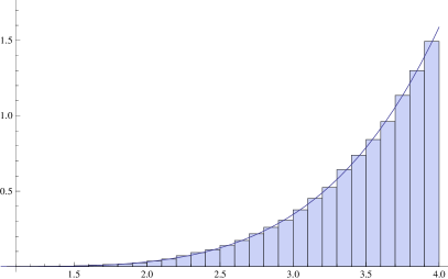
Figure 1. The distribution of the largest singular value as sampled from the PDF (4.5) using the Metropolis algorithm with $5\times 10^{5}$ steps, compared against the theoretical value (4.7). Here $R=4$.

The proposed configuration $\{\tilde{\sigma}_{l}\}$ is immediately rejected if the ordering $R>\tilde{\sigma}_{1}>\cdots>\tilde{\sigma}_{N}>0$ is violated, and the previous configuration is repeated. Otherwise one implements the Metropolis-Hastings rule that the configuration is rejected, and thus the previous configuration is repeated, with probability $1-p$, where

$$p={\rm min}\,\Big{(}{\tilde{\sigma}_{N}\over\sigma_{N}}e^{-(E(\{\tilde{\sigma}_{l}\})-E(\{\sigma_{l}\})},1\Big{)}$$ (4.6)

(the factor $\tilde{\sigma}_{N}/\sigma_{N}$ results from implementing the delta function constraint as in (4.5)).

In the case $N=3$ a test on this methodology is to use it to estimate the distribution of the largest singular value $\sigma_{1}$. According to the definition (2.14) and (2.22), the probability density function for $\sigma_{1}$, $p_{3}(s)$ say, is given by

$$p_{3}(s)={d\over ds}{J_{3}(s)\over J_{s}(R)}={{1\over 4}(s^{5}+s^{-7})-(s^{2}+s^{-4})+{3\over 2s}\over{1\over 24}(R^{6}-R^{-6})-{1\over 3}(R^{3}-R^{-3})+{3\over 2}\log R},$$ (4.7)

for $R>s>1$, and $p_{3}(s)=0$ otherwise. This test was carried out (using $\gamma={\rm N}[0,1]$ in the update, and choosing $R=4$), and excellent agreement found as exhibited in Figure 1.

4.2. Random lattices

Matrices in $M\in{\rm SL}_{N}(\mathbb{R})$ relate to lattices. To see this, one adopts a viewpoint common in linear algebra that the columns of $M$ are to be regarded as vectors in $\mathbb{R}^{N}$, denoted $\vec{m}_{1},\vec{m}_{2},\dots,\vec{m}_{N}$ say. Associated with the vectors $\{\vec{m}_{j}\}_{j=1,\dots,N}$ is the lattice

$$\Big{\{}\vec{y}:\vec{y}=\sum_{j=1}^{N}n_{j}\vec{m}_{j},\quad n_{j}\in\mathbb{Z}\>(j=1,\dots,N)\Big{\}}.$$

Equivalently, $M$ specifies a unit cell of the lattice

$$\Big{\{}\vec{x}:\vec{x}=\sum_{j=1}^{N}\alpha_{j}\vec{m}_{j},\quad 0\leq\alpha_{j}\leq 1\Big{\}}.$$ (4.8)

Due to the requirement that $\det M=1$, this has unit volume.

An important point is that matrices of the form $M\Lambda$ for $\Lambda\in{\rm SL}_{N}(\mathbb{Z})$ (i.e. the set of $N\times N$ matrices with unit determinant and integer coefficients) generate the same lattice, and moreover it is easy to verify that for a matrix $M^{\prime}\in{\rm SL}_{N}(\mathbb{R})$ to generate the same lattice as $M$, it must be that there is a $\Lambda\in{\rm SL}_{N}^{\pm}(\mathbb{Z})$ (we use this notation for the set of $N\times N$ matrices with integer coefficients and determinant $\pm 1$) such that $M^{\prime}=M\Lambda$. Attention is thus drawn to the quotient space ${\rm SL}_{N}(\mathbb{R})/{\rm SL}_{N}(\mathbb{Z})$, which is to be thought of as the space of unimodular lattices.

Crucial to the understanding of ${\rm SL}_{N}(\mathbb{R})/{\rm SL}_{N}(\mathbb{Z})$ is the notion of a fundamental domain $F\subset{\rm SL}_{N}(\mathbb{R})$. Such a domain ($F$ is not unique) has the defining properties that ${\rm SL}_{N}(\mathbb{R})=\cup_{\Lambda\in{\rm SL}_{N}(\mathbb{Z})}F\Lambda$ and also $F\Lambda\cap F$ is empty for $\Lambda$ not equal to the identity. It follows that up to possible boundary points $F$ is isomorphic to the quotient space itself.

One way to specify a fundamental domain relates in an essential way to choosing a distinguished basis for the underlying lattice. Following [29], the qualities one is seeking is to choose a basis made of reasonably short vectors which are almost orthogonal. In particular, a basis $\{\mathbf{b}_{1},\dots,\mathbf{b}_{N}\}$ is said to be Minkowski reduced if for all $1\leq i\leq N$, $\mathbf{b}_{i}$ has minimal norm among all lattice vectors $\mathbf{v}$ such that $\{\mathbf{b}_{1},\dots,\mathbf{b}_{i-1},\mathbf{v}\}$ can be extended to a basis. In this definition, the dimensions $N\leq 4$ are special: only then is it that the length of $\mathbf{b}_{i}$ must coincide with the so-called $i$-th minimum, defined as the radius of the smallest closed ball centred at the origin and containing $i$ or more linearly independent lattice vectors.

For $N=2$ it is almost immediate that $\{\mathbf{b}_{1},\mathbf{b}_{2}\}$ is Minkowski reduced if

$$||\mathbf{b}_{2}||\geq||\mathbf{b}_{1}||,\quad 2|\mathbf{b}_{1}\cdot\mathbf{b}_{2}|\leq||\mathbf{b}_{1}||^{2},$$ (4.9)

as the second inequality is equivalent to requiring that $||\mathbf{b}_{2}+n\mathbf{b}_{1}||\geq||\mathbf{b}_{2}||$ for all $n\in\mathbb{Z}$. For $N=3$, the definition of a Minkowski reduced basis in terms of the $i$-th minimum inequalities reads

$$||\mathbf{b}_{3}||\geq||\mathbf{b}_{2}||\geq||\mathbf{b}_{1}||,\quad||\mathbf{b}_{2}+n_{1}\mathbf{b}_{1}||\geq||\mathbf{b}_{2}||,\quad||\mathbf{b}_{3}+n_{2}\mathbf{b}_{2}+n_{1}\mathbf{b}_{1}||\geq||\mathbf{b}_{3}||$$ (4.10)

for all $n_{1},n_{2}\in\mathbb{Z}$.

A natural question is to specify the distributions of the lengths of the Minkowski reduced lattice vectors, and/or the first $k$ linearly independent shortest lattice vectors, as well as the angles between them when the lattice is chosen at random in the sense that the matrix of basis vectors is an element of ${\rm SL}_{N}(\mathbb{R})$ with Haar measure. By using our ability to sample the latter (when restricted to have bounded norm) we will show in the cases $N=3$ these distributions can be approximated by combining the sampling with a lattice reduction algorithm [34]. In the case $N=2$ analytical calculations are possible, and uniform sampling together with the Lagrange–Gauss algorithm for two-dimensional lattice reduction can be used to illustrate the results. We will take up this task first, before presenting our results for $N=3$. We conclude with a brief discussion of the situation in the $N\to\infty$ limit.

4.3. The case $N=2$

With $N=2$ the Haar measure for ${\rm SL}_{N}(\mathbb{R})$ can be parametrised in terms of variables simply related to the inequalities (4.9). One first notes that for general $N$, each $M\in{\rm SL}_{N}(\mathbb{R})$ can be decomposed $M=QR$, where $Q$ is a real orthogonal matrix with determinant $+1$ and $R$ is an upper triangular matrix with diagonal entries all positive. This decomposition is a matrix form of the Gram-Schmidt algorithm reducing the columns of $M$ to an orthonormal basis. From the viewpoint of the space of unimodular lattices, $Q$ acts as a rotation, and this does not alter the lengths of the reduced lattice vectors or the angles between them. It is well known in random matrix theory [28, 26, 5] that the volume element for the change of variables from the elements of $M$ to $Q$ and $R$ is

$$(dM)=\prod_{l=1}^{N}r_{ll}^{N-l}(dR)(Q^{T}dQ),$$ (4.11)

where $(Q^{T}dQ)$ is the invariant measure on SO$(N)$ as identified by Hurwitz [13].

In the case $N=2$ we have

$$R=\begin{bmatrix}r_{11}&r_{12}\\ 0&r_{22}\end{bmatrix},\qquad r_{22}=1/r_{11}.$$ (4.12)

With the lattice rotated so that $\mathbf{b}_{1}$ is chose to lie along the positive $x$-axis, we see from (4.12) that $\mathbf{b}_{1}=(r_{11},0)$ and $\mathbf{b}_{2}=(r_{12},r_{22})$, and thus the inequalities (4.9) read

$$r_{12}^{2}+r_{22}^{2}\geq r_{11}^{2},\qquad 2|r_{12}|\leq r_{11}.$$

From (4.11) and the fact that for $N=2$ we have $\int(Q^{T}dQ)=2\pi$, as follows from (2.8) multiplied by $1/2$ to account for $Q\in{\rm SO}(N)$, the volume element of the variables $\{r_{11},r_{12},r_{22}\}$ is thus seen to be equal to

$$2\pi\chi_{r_{12}^{2}+r_{22}^{2}\geq r_{11}^{2}}\chi_{2|r_{12}|\leq r_{11}}r_{11}\delta(1-r_{11}r_{22})\,dr_{11}dr_{12}dr_{22}.$$

After integration over $r_{22}$ this reduces to

$$2\pi\chi_{r_{11}/2\geq|r_{12}|\geq A_{r_{11}}(r_{11}^{2}-1/r_{11}^{2})^{1/2}}dr_{11}dr_{12},$$ (4.13)

where $A_{r}=1$ for $r\geq 1$, and $A_{r}=0$ otherwise. The sought statistical data can now readily be computed.

Proposition 4.2.

Let vol$\,\tilde{\Gamma}$ denote the volume corresponding to (4.13). We have

$${\rm vol}\,\tilde{\Gamma}={\pi^{2}\over 3}.$$ (4.14)

The probability density function of the length of the shortest lattice vector $\mathbf{b}_{1}$ is given by

$${12\over\pi}\Big{(}{s\over 2}-\chi_{s>1}(s^{2}-1/s^{2})^{1/2}\Big{)},\qquad 0<s<(4/3)^{1/4}.$$ (4.15)

The probability density function of the second shortest basis vector $\mathbf{b}_{2}$ is given by

$${12\over\pi s}\Big{(}(s^{4}-1)^{1/2}\chi_{1<s<(4/3)^{1/4}}+(2s^{2}(s^{2}-(s^{4}-1)^{1/2})-1)^{1/2})\chi_{(4/3)^{1/4}<s<\infty}\Big{)}.$$ (4.16)

The probability density function of $\cos\theta$, where $\theta$ is the angle between $\mathbf{b}_{1}$ and $\mathbf{b}_{2}$ is

$$-{3\over 2\pi}{\log(4s^{2})\over(1-s^{2})^{1/2}},\qquad 0<|s|<1/2.$$ (4.17)

Proof.  The inequality in (4.13) tells us that the maximum value of $r_{11}$ occurs when $r_{11}/2=(r_{11}^{2}-1/r_{11}^{2})^{1/2}$ and thus $r_{11}^{4}=3/4$. Using this fact, it follows that

$${\rm vol}\,\tilde{\Gamma}=4\pi\Big{(}\int_{1}^{(4/3)^{1/4}}\Big{(}{r\over 2}-(r^{2}-1/r^{2})^{1/2}\Big{)}\,dr+\int_{0}^{1}{r\over 2}\,dr\Big{)}.$$

Evaluating the integrals gives (4.14).

For the distribution of the length of the shortest vector, we know from the text below (4.12) that this length is equal to $r_{11}$. Integrating (4.13) over $r_{12}$, and normalising using (4.14), we obtain (4.15).

According to the text below (4.12) the length of the second shortest linearly independent vector is equal to $(r_{12}^{2}+1/r_{11}^{2})^{1/2}$. Setting this equal to $s$, the inequalities in (4.13) require that $1/s<r_{11}<\sqrt{2}(s^{2}-(s^{4}-1)^{1/2})^{1/2}$, while $dr_{12}=(t/r_{12})dt$. Thus, after changing variables from $r_{12}$ to $s$ in (4.12), our task is compute

$$\int_{1/s}^{\sqrt{2}(s^{2}-(s^{4}-1)^{1/2})^{1/2}}{sr\over(r^{2}s^{2}-1)^{1/2}}\,dr.$$

Doing this and normalising gives (4.16).

The text below (4.12) tells us that $\cos\theta=r_{12}/(r_{12}^{2}+(1/r_{11})^{2})^{1/2}$. Denoting this by $s$, the inequalities in (4.13) require that $(4s^{2}/(1-s^{2}))^{1/4}<r_{11}<1/(1-s^{2})^{1/4}$ and $0<|s|<1/2$. Also, $dr_{12}=1/(r_{11}(1-s^{2})^{3/2})\,ds$. Thus, after changing variables from $r_{12}$ to $s$ in (4.12), our remaining task is to compute

$$\int_{(4s^{2}/(1-s^{2}))^{1/4}}^{1/(1-s^{2})^{1/4}}{1\over r}\,dr.$$

Doing this, and after appropriate normalisation, (4.17) results. $\square$

Remark 4.3.

The volume (4.14) is equal to twice the value of ${\rm vol}\,\Gamma$ in the case $N=2$ as given by (1.1). This can be understood due to (1.1) relating to the fundamental domain of the quotient ${\rm SL}_{N}(\mathbb{R})/{\rm SL}_{N}(\mathbb{Z})$, whereas in (4.14) the quotient is ${\rm SL}_{N}(\mathbb{R})/{\rm SL}_{N}^{\pm}(\mathbb{Z})$, where ${\rm SL}_{N}^{\pm}(\mathbb{Z})$ is the set of all $N\times N$ matrices with integer entries and determinant equal to $\pm 1$.

Remark 4.4.

According to (4.15) the maximum allowed value of the length of the shortest vector is $(4/3)^{1/4}$. Suppose that the other basis vector also has this length. Then, for the resulting unit cell to have area unity, the angle between the two vectors must be $\pi/3$ or $4\pi/3$ and so the cosine of the angle must be $\pm 1/2$, which is the largest value in magnitude permitted by (4.17). This corresponds to the triangular, or equivalently hexagonal, lattice.

Remark 4.5.

Consider a punctured disk of radius $0<R<1$ about the origin. According to Proposition 4.2 this disk will contain only the shortest lattice vector and integer multiples $\pm\mathbf{b}_{1},\pm 2\mathbf{b}_{1},\dots,\pm m\mathbf{b}_{1}$, where $m||\mathbf{b}_{1}||<R\leq(m+1)||\mathbf{b}_{1}||$, or equivalently $m=\lfloor R/||\mathbf{b}_{1}||\rfloor$. Thus, with $\Omega(R)$ denoting the expected number of lattice vectors in this punctured disk, making use of (4.15) shows

$$\Omega(R)={12\over\pi}\int_{0}^{R}\Big{\lfloor}{R\over s}\Big{\rfloor}s\,ds={12R^{2}\over\pi}\int_{0}^{1}\Big{\lfloor}{1\over s}\Big{\rfloor}s\,ds.$$ (4.18)

The latter integral can be written as a sum and evaluated according to

$$\int_{0}^{1}\Big{\lfloor}{1\over s}\Big{\rfloor}s\,ds=\sum_{p=1}^{\infty}p\int_{1/(1+p)}^{1/p}r\,dr={1\over 2}\sum_{p=1}^{\infty}{1\over p^{2}}={\pi^{2}\over 12},$$ (4.19)

where the second equality follows by evaluating the integral and simple manipulation of the resulting summation. Hence, for $R<1$, $\Omega(R)=\pi R^{2}$, which is the area of the corresponding disk. This result, which remains valid for all $R>0$, is a well known consequence of Siegel’s mean value theorem for lattices; for a readable account see [30].

Remark 4.6.

Integration over the invariant measure for SL${}_{2}(\mathbb{R})/{\rm SL}_{2}(\mathbb{Z})$ has been carried out in the recent work [25] to obtain the explicit functional form of the distribution of certain scaled diameters for random $2k$-regular circulant graphs with $k=2$. A number of the required integrals had earlier appeared in the works [22] and [38]. Our (4.15) in fact has an interpretation in the context of [38], which relates to the asymptotics of certain random linear congruences mod $p$, as $p\to\infty$. Specifically, it gives the explicit value of $c_{1}$ in the special case $n=2$, $\Omega$ a disk centred at the origin of [38, Theorem 2], while restricting the radius of the disk to less than 1, our Remark 4.5 implicitly contains the formula for $c_{3},c_{5},\dots$ as well (each $c_{2j}$ vanishes by symmetry). In [38, Prop. 3] the analogous formula for $c_{1},c_{3},c_{5}$ in the case of a rectangle in place of the disk, and also for $c_{7},c_{9},\dots$ in the case of a sufficiently small rectangle were given, while [38, Section 8] ends by comparing with Siegel’s mean value formula analogous to our Remark 4.5.

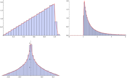
Figure 2. Numerically generated histograms for the distribution of the length of the shortest vector, the length of the second shortest linearly independent vector, and the cosine of the angle between these vectors for Haar distributed matrices in the fundamental domain, obtained by applying Lagrange–Gauss lattice reduction to $10^{5}$ Haar distributed elements from Sl$(2,\mathbb{R})$ with larges singular value less than 100. The red curves are the theoretical predictions from Proposition 4.2

We would like to illustrate the results of Proposition 4.2 by first generating matrices from SL${}_{2}(\mathbb{R})$ with Haar measure, and then using Lagrange–Gauss reduction of the corresponding lattice to the fundamental domain. We generate the matrices in the form of their singular value decomposition (2.5), with $O_{1}$ and $O_{2}$ chosen with Haar measure from O$(N)$, and the singular values generated according to the method of §4.3. The matrices from O$(N)$ can be generated by converting to Gram–Schmidt form the columns of an $N\times N$ matrix of independent standard real Gaussians. In the case $N=2$, the result of Proposition 4.1 tells us how to generate the singular values, provided the largest singular value is no bigger than $R$. For each matrix $M$ so generated, the Lagrange–Gauss algorithm (see e.g. [3]) is applied so as to reduce, using elements of ${\rm SL}_{2}^{\pm}(\mathbb{Z})$, the column vectors of $M$ down to the fundamental domain. This is a simple and efficient task. Each $M$ can be viewed as consisting of two column vectors. To initialise the algorithm, let $\mathbf{u}$ denote the shortest, and $\mathbf{v}$ the longest column vector. Step 1 is to calculate the scalar $\alpha=\lfloor(\mathbf{u}\cdot\mathbf{v})/||\mathbf{u}||^{2}\rceil$, with $\lfloor\cdot\rceil$ denoting the closest integer function, and from this define the vector $\mathbf{r}=\mathbf{v}-\alpha\mathbf{u}$. Step 2 is to update the shortest and longest vectors by defining $\mathbf{v}:=\mathbf{u}$, $\mathbf{u}:=\mathbf{r}$. If indeed $||\mathbf{u}||<||\mathbf{v}||$, steps 1 and 2 are repeated. If not, the process ends and returns the final updated values of $(\mathbf{v},\mathbf{u}$) as the columns of $M$ reduced to the fundamental domain, with the first column corresponding to the lattice vector with the shortest length. It is known (see e.g. [29]) that the total number of steps required is bounded by a constant times the square of the logarithm of the longest length vector in $M$. Repeating this process many times allows us to form histograms approximating the distribution of the shortest and longest basis vectors, and the cosine of the angle between them. The results are displayed in Figure 2, showing excellent agreement between the theoretical and simulated distributions.

4.4. The case $N=3$

As written, the conditions (4.10) for a Minkowski reduced basis in the case $N=3$ consist of an infinite number of inequalities. It was proved by Minkowski himself that in fact a finite number of equalities suffice, the explicit form of which can be found in [39, §4.4.3] for example. On the other hand, it does not seem possible to carry out the integrations needed to compute the exact form of the distributions of the lengths and pairwise angles of the basis vectors. Nonetheless the numerical approach used above for $N=2$ can be generalised.

The first step is to use the Metropolis Monte Carlo algorithm as detailed in the text below Proposition 4.1 to generate the singular values of matrices from SL${}_{3}(\mathbb{R})$ with Haar measure and bounded norm. Matrices $M$ from SL${}_{3}(\mathbb{R})$ with Haar measure can then be generated by using (2.5), as discussed in the second sentence of the paragraph below Remark 4.3. The task of transforming the columns of $M$ in the case $N=3$ to a Minkowski reduced basis can be carried out using an algorithm due to Semaev [34]. As input are three basis vectors $\mathbf{b}_{1}$, $\mathbf{b}_{2}$, $\mathbf{b}_{3}$, ordered so that $|\mathbf{b}_{1}|\leq|\mathbf{b}_{2}|\leq|\mathbf{b}_{3}|$. Step 1 applies the Lagrange–Gauss algorithm to $\mathbf{b}_{1},\mathbf{b}_{2}$ and updates the vectors accordingly. With $C=1-(\mathbf{b}_{1}\cdot\mathbf{b}_{2})^{2}/(||\mathbf{b}_{1}||^{2}||\mathbf{b}_{2}||^{2})$ and

$$x_{2}:=-\Big{\lfloor}{1\over C}\Big{(}{\mathbf{b}_{2}\cdot\mathbf{b}_{3}\over||\mathbf{b}_{2}||^{2}}-{\mathbf{b}_{1}\cdot\mathbf{b}_{2}\over||\mathbf{b}_{2}||^{2}}{\mathbf{b}_{1}\cdot\mathbf{b}_{3}\over||\mathbf{b}_{1}||^{2}}\Big{)}\Big{\rceil},\quad x_{1}:=-\Big{\lfloor}{1\over C}\Big{(}{\mathbf{b}_{1}\cdot\mathbf{b}_{3}\over||\mathbf{b}_{1}||^{2}}-{\mathbf{b}_{1}\cdot\mathbf{b}_{2}\over||\mathbf{b}_{1}||^{2}}{\mathbf{b}_{2}\cdot\mathbf{b}_{3}\over||\mathbf{b}_{2}||^{2}}\Big{)}\Big{\rceil},$$

for step 2 set $\mathbf{a}=\mathbf{b}_{3}+x_{2}\mathbf{b}_{2}+x_{1}\mathbf{b}_{1}$. Finally, in step 3, the process terminates if $||\mathbf{a}||\geq||\mathbf{b}_{3}||$. Otherwise, $\mathbf{b}_{3}$ is replaced by $\mathbf{a}$, the updated vectors $\mathbf{b}_{1}$, $\mathbf{b}_{2}$, $\mathbf{b}_{3}$ are ordered as in the input, and the algorithm returns to step 1. It is proved in [34] that the total number of steps required is bounded by a constant times $\log(||\mathbf{b}_{3}||/||\mathbf{v}_{1}||)+1)\log||\mathbf{b}_{3}||$, where $\mathbf{v}_{1}$ denotes the shortest vector in the reduced basis.

Implementing this procedure allows us to efficiently generate a large number of Minkowski reduced basis vectors in $\mathbf{R}^{3}$ with Haar measure — which correspond to vectors with the lengths equal to the first three successive minima — and to form histograms approximating the distribution of the lengths of these vectors, and the cosines of their pairwise angles; see Figure 3. It appears in the graphs that the largest permitted value of the shortest vector is, as for the $N=2$ case, $(4/3)^{1/4}$, which is in keeping with the face centred cubic lattice — viewed as alternate layers of hexagonal lattices — giving the most efficient packing of spheres. The smallest permitted value of the second shortest linearly independent vector lies in the interval $(0,3,0,35)$, while again as for the $N=2$ case, the third shortest linearly independent vector has shortest allowed length of 1 (corresponding to the simple cubic lattice). The cosine of the angle between the shortest and second shortest basis vectors has magnitude less than or equal to $1/2$, as for $N=2$, while this magnitude for the shortest and third shortest pair, and the second and third shortest pair appears to be less than or equal to $1/\sqrt{3}$. It remains as a challenge to further quantify these observation, and moreover to give an analytic description of the distributions.

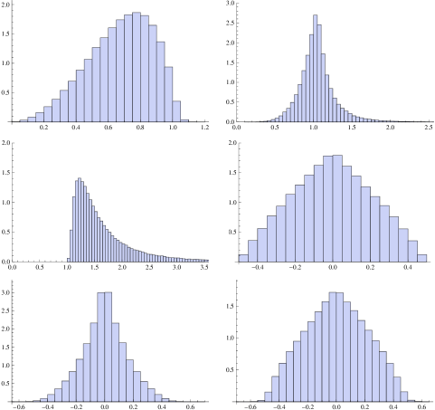
Figure 3. We denote by $\mathbf{v}_{1}$, $\mathbf{v}_{2}$, $\mathbf{v}_{3}$, the three Minkowski reduced basis vectors corresponding to a Haar distributed element of SL${}_{3}(\mathbb{R})$ and largest singular value bounded by $R=100$. The histrograms then correspond to the distribution of the length of $\mathbf{v}_{1}$, $\mathbf{v}_{2}$, $\mathbf{v}_{3}$, and the cosines of the angle between the pairs $(\mathbf{v}_{1},\mathbf{v}_{2})$, $(\mathbf{v}_{1},\mathbf{v}_{3})$ and $(\mathbf{v}_{2},\mathbf{v}_{3})$ respectively, with the vectors as generated by the procedure detailed in the text.

One front on which such progress can be made is in relation to the small distance form of the probability density function ,$p_{1}(s)$, say for the shortest basis vector. In the notation of Remark 4.5, for $N=3$ Siegel’s mean value theorem tells us that $\Omega(R)={4\over 3}\pi R^{3}$. On the other hand, trialling $p_{1}(s)=Cs^{2}$ for $s$ smaller than the minimum allowed value of the second smallest basis vector gives, according to reasoning of (4.18)

$$\Omega(R)=2C\int_{0}^{R}\Big{\lfloor}{R\over s}\Big{\rfloor}s^{2}\,ds=2CR^{3}\int_{0}^{1}\Big{\lfloor}{1\over s}\Big{\rfloor}s^{2}\,ds.$$

Evaluating the integral according to the method of (4.19) shows $\Omega(R)=2C\zeta(3)R^{3}/3$ and thus $C=2\pi/\zeta(3)$. The functional form $p_{1}(s)=2\pi s^{3}/\zeta(3)$ gives seemingly perfect agreement with the first histogram of Figure 3 in the range $0\leq s\leq\mu$, for $\mu\approx 1/3$.

We remark that the invariant measure on the space of unimodular lattices for $N=3$ plays a fundamental role in the studies [23, 24] relating to the periodic Lorenz gas.

4.5. The $N\to\infty$ limit

The $N=3$ lattice reduction algorithm of Semaev [34] has been described in [29] as a greedy version of two-dimensional Lagrange–Gauss lattice reduction — it used reduced vectors in dimension $N-1$ to obtain the reduced basis in dimension $N$. However only for $N\leq 4$ does the greedy algorithm produce a Minkowski reduced basis [29]. In higher dimensions this latter task is both complicated and costly. Instead approximate lattice reduction is used, with the best known method being the LLL algorithm, which guarantees the shortest vector up to a factor bounded by $\beta^{(N-1)/2}$, $\beta\approx 4/3$. Thus there is a deterioration as $N$ gets large. On the other hand, it is in the limit $N\to\infty$ that an analytic description of the distribution of the shortest lattice vectors and their pairwise angles again becomes possible for lattices corresponding to Haar distributed SL${}_{N}(\mathbb{R})$ matrices [32, 36, 37, 17, 18].

Specifically, let $0<\ell_{1}\leq\ell_{2}\leq\cdots$ denote the ordered sequence of the lengths of the nonzero lattice vectors, with each pair $\pm\mathbf{v}$ counted as one. Define $\nu_{j}:=\pi^{N/2}l_{j}^{N}/\Gamma(N/2+1)$, which has the interpretation as the volume of an $N$-dimensional ball of radius $\ell_{j}$. A result of [32], as generalised in [36, 18], gives that with $k$ fixed and $N\to\infty$, the sequence $\{\nu_{l}\}_{l=1}^{k}$ is distributed as a Poisson process on $\mathbb{R}^{+}$ with intensity $1/2$. And with $\varphi_{jk}$, $0\leq\varphi_{jk}\leq\pi/2$, denoting the angle between the pairs of vectors with length $\ell_{j}$ and $\ell_{k}$, it is proved in [37] that each $\tilde{\varphi}_{jk}:=\sqrt{N}(\pi/2-\varphi_{jk})$ has the distribution of the absolute value of a standard Gaussian random variable.

Generally the $N\to\infty$ limit of random lattices corresponding to Haar distributed SL${}_{N}(\mathbb{R})$ matrices is of interest from a number of different perspective in mathematical physics; see e.g. [21]. The challenge suggested by the present work is to implement sufficiently accurate lattice reduction in high enough dimension so that histograms analogous to those of Figures 2 and 3 can be generated to illustrate the results summarised in the previous paragraph.

References

- [1] G. Akemann and Z. Burda, Universal microscopic correlations for products of independent Ginibre matrices, J. Phys. A 45 (2012), 465210.
- [2] G. Akemann, J.R. Ipsen, and M. Kieburg, Products of rectangular random matrices: Singular values and progressive scattering, Phys. Rev. E 88 (2013), 052118.
- [3] M.R. Bremner, Lattice basis reduction: an introduction to the LLL algorithm and its applications, CRC Press, Boca Raton, FL, 2012.
- [4] P. Diaconis and P.J. Forrester, A. Hurwitz and the origin of random matrix theory in mathematics, arXiv:1512.09229, 2015.
- [5] A. Edelman and N. Raj Rao, Random matrix theory, Acta Numerica (A. Iserles, ed.), vol. 14, Cambridge University Press, Cambridge, 2005.
- [6] P.J. Forrester, Log-gases and random matrices, Princeton University Press, Princeton, NJ, 2010.
- [7] P.J. Forrester and J.P. Keating, Singularity dominated strong fluctuations for some random matrix averages, Commun. Math. Phys. 250 (2004), 119–131.
- [8] P.J. Forrester and E.M. Rains, A Fuchsian matrix differential equation for Selberg correlation integrals, Commun. Math. Phys. (2012), 309, (2012), 771–792.
- [9] P.J. Forrester and S.O. Warnaar, The importance of the Selberg integral, Bull. Am. Math. Soc. 45 (2008), 489–534.
- [10] E. Fucks and I. Rivin, Generic thinness in finitely generated subgroups of SL, arXiv:1506.01735.
- [11] D. Goldstein and A.Mayer, On the equidistribution of Hecke points, Forum Math. 15 (2003), 165–189.
- [12] A. Hardy, Average characteristic polynomials of determinant point processes, Ann. L’Institut Henri Poincaré – Prob. et Stat. 51 (2015), 283–303.
- [13] A. Hurwitz, Über die Erzeugung der Invarianten durch Integration, Nachr. Ges. Wiss. Göttingen (1897), 71–90.
- [14] H. Jack, The asymptotic value of the volume of a certain set of matrices, Proc. Edinburgh Math. Soc. 15 (1967), 209–213.
- [15] H. Jack and A.M. Macbeath, The volume of a certain set of matrices, Math. Proc. Camb. Phil. Soc. 55 (1959), 213–223.
- [16] M. Kieburg, A.B.J. Kuijlaars and D. Stivigny Singular value statistics of matrix products with truncated unitary matrices, arXiv:1501.03910.
- [17] S. Kim, On the shape of a high-dimensional random lattice, Ph.D. thesis, Stanford University, 2015.
- [18] by same author, On the distribution of lengths of short vectors in a random lattice, Mathematische Zeitschrift 282 (2016), 1117–1126.
- [19] A.M. Macbeath and C.A. Rogers, A modified form of siegel’s mean value theorem, Math. Proc. Camb. Phil. Soc. 51 (1955), 565–576.
- [20] by same author, Siegel’s mean value theorem in the geometry of numbers, Math. Proc. Camb. Phil. Soc. 54 (1958), 139–151.
- [21] J. Marklof, The -point correlations between value of a linear form, Ergod. Th. & Dyn. Systems 20 (2000), 1127–1172.
- [22] J. Marklof and A. Strömbergsson, Kinetic transport in the two-dimensional periodic Lorentz gas, Nonlinearity 21 (2008), 1413 -1422.
- [23] by same author, The distribution of free path lengths in the periodic Lorentz gas and related lattice point problems, Ann. Math. 172 (2010): 1949–2033.
- [24] by same author, The periodic Lorentz gas in the Boltzmann-Grad limit: asymptotic estimates, Geometric and Functional Analysis 21 (2011) 560–647.
- [25] by same author, Diameters of random circulant graphs, Combinatorica 33 (2013) 429-466.
- [26] A.M. Mathai, Jacobians of matrix transformations and functions of matrix arguments, World Scientific, Singapore, 1997.
- [27] H. Minkowski, Diskontinuitätsbereich für arithmetische äquivalenz, J. Reine Angew. Math. 129 (1905), 220–274.
- [28] R.J. Muirhead, Aspects of multivariate statistical theory, Wiley, New York, 1982.
- [29] P.Q. Nguyen and D. Stehlé, Low-dimensional lattice basis reduction revisited, Algorithmic number theory, Lecture notes in computer science, vol. 3076, Springer Berlin Heidelberg, 2001, pp. 338–357.
- [30] G. Parisi, On the most compact regular lattices in large dimensions: A statistical mechanical approach, J. Stat. Phys. 132 (2008), 207–234.
- [31] I. Rivin, How to pick a random integer matrix? (and other questions), Math. Computation 85 (2016), 783–797.
- [32] C.A. Rogers, The moments of the number of points of a lattice in a bounded set, Phil. Trans. R. Soc. Lond. A 248 (1955), 225–251.
- [33] A. Selberg, Bemerkninger om et multipelt integral, Norsk. Mat. Tidsskr. 24 (1944), 71–78.
- [34] I. Semaev, A 3-dimensional lattice reduction algorithm, Proc. of CALC ’01 (P. Huber and M. Rosenblatt, eds.), Lecture notes in computer science, vol. 2146, Springer-Verlag, 2001, pp. 183–193.
- [35] C.L. Siegel, A mean value theorem in geometry of numbers, Ann. Math. 46 (1945), 340–347.
- [36] A. Södergren, On the Poisson distribution of lengths of lattice vectors in a random lattice, Mathematische Zeitschrift 269 (2011), 945–954.
- [37] by same author, On the distribution of angles between the shortest vectors in a random lattice, J. London Math. Soc. 84 (2011), 749–764.
- [38] A. Strömbergsson and A. Venkatesh, Small solutions to linear congruences and Hecke equidistribution, Acta Arith., 118 (2005), 41-78.
- [39] A. Terras, Harmonic analysis on symmetric spaces and applications, vol. 2, Springer-Verlag, Birlin, 1988.
- [40] P. Sarak W. Duke and Z. Rudnick, Density of integer points on affine homogeneous varieties, Duke Math. J. 81 (1993), 143–179.
- [41] K. Zyczkowski and H.-J. Sommers, Induced measures in the space of mixed quantum states, J. Phys. A 34 (2001), 7111–7125.