Rescuing a Quantum Phase Transition with Quantum Noise

Abstract

We show that placing a quantum system in contact with an environment can enhance non-Fermi-liquid correlations, rather than destroy quantum effects as is typical. The system consists of two quantum dots in series with two leads; the highly resistive leads couple charge flow through the dots to the electromagnetic environment, the source of quantum noise. While the charge transport inhibits a quantum phase transition, the quantum noise reduces charge transport and restores the transition. We find a non-Fermi-liquid intermediate fixed point for all strengths of the noise. For strong noise, it is similar to the intermediate fixed point of the two-impurity Kondo model.

Quantum fluctuations and coherence are key distinguishing ingredients in quantum matter. Two phenomena to which they give rise, for instance, are quantum phase transitions Carr (2011); Vojta (2006), changes in the ground state of a system driven by its quantum fluctuations, and quantum noise Leggett et al. (1987); Weiss (2012); Ingold and Nazarov (1992), the effect on the system of quantum fluctuations in its environment, for no system is truly isolated. Understanding the intersection of these two topics—the effects of quantum noise on quantum phase transitions—is important for understanding quantum matter. It is natural to suppose that decoherence produced by the noise will suppress quantum effects, and in particular inhibit or destroy a quantum critical state. Indeed, a variety of calculations demonstrate this in both equilibrium Leggett et al. (1987); Weiss (2012); Kapitulnik et al. (2001); Le Hur (2004); Cazalilla et al. (2006); Chung et al. (2007); Hoyos and Vojta (2008); Poletti et al. (2012); Cai and Barthel (2013); *CaiBoseLiqPRL14 and non-equilibrium Dalla Torre et al. (2012); *DallaTorreNP10; Foss-Feig et al. (2013); Chung et al. (2013); Joshi et al. (2013); Sieberer et al. (2013) contexts. There are also a few known cases that do not follow this rule Werner et al. (2005); Nagy and Domokos (2015); Marino and Diehl (2016). Here, we present a striking counter-example to the notion that environmental noise necessarily harms quantum many-body effects: in the system we study, the addition of (equilibrium) quantum noise stabilizes a non-Fermi liquid quantum critical state.

We discuss the phase diagram of two quantum dots connected to two leads in the presence of environmental quantum noise. The noiseless model has a quantum phase transition that is transformed into a crossover by charge transport across the double dot. We show that quantum fluctuations of the field associated with the source and drain voltage counteract this charge transport. The competition between these two processes restores the delicate balance of the quantum critical state. The result is that the quantum phase transition is rescued from the undesired crossover for any strength of the noise.

Our double quantum dot setup is shown schematically in Fig. 1: two small dots are in series between two leads, labeled $L$ (left) or $R$ (right). The leads are resistive, thereby coupling the electrons to an ohmic electromagnetic environment. Experimentally, small double dots have been studied in several materials Jeong et al. (2001); Chorley et al. (2012); Keller et al. (2014); Bork et al. (2011); Spinelli et al. (2015), and the effect of the environment on transport in simpler systems has been recently studied in detail Parmentier et al. (2011); Mebrahtu et al. (2012, 2013); Jezouin et al. (2013), including transport through a single quantum dot Mebrahtu et al. (2012, 2013). Thus, all the necessary ingredients for an experimental study of our system are available.

Model for dots and leads—The model has three parts: leads, dots, and electromagnetic environment. Following standard procedures, we linearize the spectrum of each lead, notice that a one-dimensional subset of electrons couples to each dot, and represent it using chiral fermions by analytic continuation with open boundary conditions [][pp.351-368.]GogolinBook. The resulting lead Hamiltonian is the sum of four free Dirac fermions,

$$H_{\text{leads}}^{0}=\sum_{\alpha,\sigma}\int_{-\infty}^{\infty}\!\!dx\,\psi_{\alpha,\sigma}^{\dagger}(x)i\partial_{x}\psi_{\alpha,\sigma}(x),$$ (1)

where $\alpha$ and $\sigma$ are the lead and spin labels and both the Fermi velocity and $\hbar$ are set to unity.

For the dots, we consider the Coulomb blockade regime in which charge fluctuations are suppressed and the electron number is odd Yu. V. Nazarov and Blanter (2009). The single-level Anderson model is suitable for each dot, as the spacing between levels in the carbon nanotube dots is large Mebrahtu et al. (2012, 2013). Each dot, then, has a low energy spin-$\frac{1}{2}$ degree of freedom, $\vec{S}_{\alpha}$. Projecting onto this low-energy subspace via a second-order Schrieffer-Wolff transformation produces two Kondo-like terms with couplings $J_{L,R}$ and a spin-spin anti-ferromagnetic interaction with coupling $K$:

$$H_{\text{dots}}=J_{L}\vec{s}_{L}(0)\cdot\vec{S}_{L}+J_{R}\vec{s}_{R}(0)\cdot\vec{S}_{R}+K\vec{S}_{L}\cdot\vec{S}_{R},$$ (2)

where $\vec{s}_{\alpha}\!=\!\psi_{\alpha}^{\dagger}(0)\vec{\sigma}\,\psi_{\alpha}(0)$ is the spin-density in the lead at the point connected to the dot. Though none of our results depend on left-right symmetry, we take $J_{L}\!=\!J_{R}$ for simplicity.

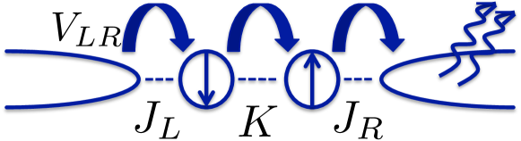
Figure 1: Schematic of the system: two quantum dots coupled to left and right leads. $J_{L,R}$ and $K$ refer to the Kondo and exchange coupling strengths, respectively. $V_{LR}$ is the strength of direct charge transport between the leads. Dissipative modes in the leads are represented by wiggly arrows.

Charge transfer between the two leads is key to the physics of this system Jones et al. (1989); Georges and Meir (1999); Zaránd et al. (2006); Sela and Affleck (2009a); Malecki et al. (2010); Jayatilaka et al. (2011). The effective hopping between the leads that arises from the third-order Schrieffer-Wolff transformation of the original Anderson model must be added Jayatilaka et al. (2011):

$$H_{LR} = V_{LR}\left[\big{(}\psi_{L\uparrow}^{\dagger}\psi_{R\uparrow}^{\,}+\psi_{R\downarrow}^{\dagger}\psi_{L\downarrow}^{\,}\big{)}S_{L}^{-}S_{R}^{+}\right.$$

$$+ \big{(}\psi_{L\uparrow}^{\dagger}\psi_{R\uparrow}^{\,}+\psi_{L\downarrow}^{\dagger}\psi_{R\downarrow}^{\,}\big{)}S_{L}^{z}S_{R}^{z}$$

$$+ \left.\big{(}\psi_{L\uparrow}^{\dagger}\psi_{R\downarrow}^{\,}-\psi_{R\uparrow}^{\dagger}\psi_{L\downarrow}^{\,}\big{)}\left(S_{L}^{z}S_{R}^{-}-S_{L}^{-}S_{R}^{z}\right)\right]+\mbox{h.c.},$$

where $x\!=\!0$ for the lead operators Sup . This form is obtained because moving an electron across the dots necessarily involves the dot spins. Much of the physics added by (Rescuing a Quantum Phase Transition with Quantum Noise) is obtained from a simpler direct hopping, $\hat{H}_{LR}=\hat{V}_{LR}\psi_{L\sigma}^{\dagger}(0)\psi_{R\sigma}^{\,}(0)+\mbox{h.c.}$ Jayatilaka et al. (2011); Malecki et al. (2011). We therefore simplify the discussion by using $\hat{H}_{LR}$ rather than $H_{LR}$ when possible Sup .

The final ingredient in our system is the “quantum noise.” Quantum fluctuations of the source and drain voltage require a quantum description of the tunneling junction Ingold and Nazarov (1992); Yu. V. Nazarov and Blanter (2009). The standard procedure is to introduce junction charge and phase fluctuation operators that are conjugate to each other and (bilinearly) coupled to modes of the ohmic environment with resistance $R$. Treating the latter as a collection of harmonic oscillators with the desired impedance, we write the environment as a free bosonic field, $H_{\varphi}^{0}\!=\!\int\frac{dx}{4\pi}(\partial_{x}\varphi)^{2}$, which is excited in a tunneling event through the charge-shift operator $e^{i\sqrt{2r}\varphi(0)}$ Ingold and Nazarov (1992). Such a shift operator is added to every term in $H_{LR}$ according to

$$\psi_{L\sigma}^{\dagger}\psi_{R\sigma}^{\,}\to e^{i\sqrt{2r}\varphi(0)}\psi_{L\sigma}^{\dagger}\psi_{R\sigma}^{\,},$$ (4)

where $r\!=\!Re^{2}/h$ is the dimensionless resistance. The environment does not modify the second-order exchange couplings Eq. (2) because those virtual processes occur on the very short time scale of the inverse charging energy Florens et al. (2007), typically smaller than the time scale of the environment. This model of noisy tunneling has been used previously in work on a resonant level Imam et al. (1994); Le Hur and Li (2005), including in our own work Mebrahtu et al. (2012, 2013); Liu et al. (2014); Zheng et al. (2014), and for a quantum dot in the Kondo regime Florens et al. (2007). In summary, the starting point of our discussion is the Hamiltonian

$$H=H_{\text{leads}}^{0}+H_{\varphi}^{0}+H_{\text{dots}}+{H}_{LR}\left(r\right).$$ (5)

Quantum phase transition or crossover?—First, we bosonize the chiral fermions describing the leads, Eq. (1), thereby introducing chiral bosonic fields $\phi_{\alpha,\sigma}$ Gogolin et al. (2004); Malecki et al. (2010); Sup . One can then see that the ultraviolet fixed point, described by $H_{\text{leads}}^{0}+H_{\varphi}^{0}$, is unstable. There are two important energy scales connected to this instability: the Kondo temperature, $T_{K}$, associated with the screening of each dot by its own lead, and the “crossover temperature,” $T^{*}\!<\!T_{K}$ Malecki et al. (2010, 2011).

To explain $T^{*}$, we start by considering $V_{LR}\!=\!0$, yielding the two-impurity Kondo model. For $T\!<\!T_{K}$, there are two Fermi-liquid phases with a critical coupling that separates them Jones et al. (1989); Affleck et al. (1995), denoted by $K_{c}$. (i) For $K\!>\!K_{c}$, the two dots become maximally entangled in a singlet state—the local-singlet phase controlled by a fixed point, denoted LSFP, with a scattering phase shift of $0$. (ii) For $K\!<\!K_{c}$, each dot becomes maximally entangled with its respective lead, forming two decoupled Kondo singlets—the Kondo phase controlled by a fixed point, denoted KFP, phase shift of $\pi/2$. The fact that the phase shifts are different implies the existence of an intermediate (unstable) fixed point Affleck et al. (1995); Maldacena and Ludwig (1997), which we call IFP₁ (see Fig. 2).

Inter-lead tunneling, $V_{LR}\!\neq\!0$, changes the behavior dramatically. In the absence of dissipation, $r\!=\!0$, it is known that $H_{LR}$ destabilizes IFP₁ Sela and Affleck (2009b); Zaránd et al. (2006); Sela and Affleck (2009a); Malecki et al. (2010); Jayatilaka et al. (2011), becoming effective below a scale $T^{*}$. The low-energy physics is described by Fermi-liquid Hamiltonians with scattering phase shift varying from $\delta\!=\!0$ to $\pi/2$ depending on the initial values of the couplings Georges and Meir (1999); Sela and Affleck (2009a); Malecki et al. (2010, 2011). The finite temperature conductance is $G=G_{0}\sin(2\delta)[1\!-\!\kappa(T/T^{*})^{2}]$, where $G_{0}\!=\!2e^{2}/h$ and $\kappa$ is non-universal. Therefore, for $T\!<\!T^{*}$, the quantum phase transition of the two-impurity Kondo model is transformed into a crossover between the Kondo and local-singlet regimes.

Quantum noise effects—Close to the KFP and LSFP, the tunneling Hamiltonian in the absence of noise, $H_{LR}$, is a marginal operator Sela and Affleck (2009a); Malecki et al. (2010, 2011): without noise, any bilinear operator that transfers charge between the leads is marginal at these two fixed points. A key effect of the noise is that the scaling dimension of such an operator increases, making it irrelevant. In the tunneling operator $H_{LR}$, the increase is caused by the exponential charge-shift operator introduced in Eq. (4). The line of Fermi-liquid fixed points existing at $r\!=\!0$ is then destroyed. The conductance around the KFP and LSFP follows from perturbation theory in the tunneling, leading to $G(T)\sim T^{2r}$ Ingold and Nazarov (1992); Kane and Fisher (1992a); *KaneFisherPRB92.

The new found stability of the Kondo and local-singlet fixed points with respect to tunneling demands once again the existence of an intermediate fixed point. We denote this “dissipative intermediate fixed point” by IFP₂, as shown in Fig. 2.

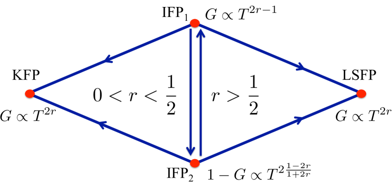
Figure 2: Stability diagram for different noise strengths $r$, and the temperature dependence of the conductance at each fixed point. The KFP and LSFP are stable for any non-zero $r$, while the nature of the IFP changes as a function of $r$. For $r\!<\!1/2$, the intermediate state is controlled by IFP₂—the fixed point that evolves from one of the $r\!=\!0$ Fermi-liquid fixed points. In contrast, for $r\!>\!1/2$, IFP₁—which evolves from the two-impurity-Kondo IFP—is relevant. For $r\!=\!1/2$ a line of fixed points connects IFP₁ to IFP₂.

IFP₂ occurs for the same value of $K$ as IFP₁, namely $K\!=\!K_{c}$, as we now show. It is known that the effect of a resistive environment on a bilinear tunneling operator is connected to the partition noise produced by the tunneling Levy Yeyati et al. (2001); Safi and Saleur (2004): when there is no partition noise, the environment is not excited by the current and so has no effect. This is the case at $K\!=\!K_{c}$: the phase shift is $\delta\!=\!\pi/4$, so the zero temperature conductance is $G\!=\!2e^{2}/h$ and the transmission is unity. Thus, there is no partition noise: from the line of $r\!=\!0$ Fermi-liquid fixed points, this fixed point survives at non-zero $r$ and is, in fact, IFP₂. We now turn to characterizing both IFP’s in detail.

Effective Hamiltonian at the intermediate fixed points—In order to derive an effective Hamiltonian at the critical coupling, $K\!=\!K_{c}$, we follow the dissipationless discussion of J. Gan in Ref. Gan (1995). First, we define new bosonic fields,

$$\phi_{c/s} = \left(\phi_{L\uparrow}\pm\phi_{L\downarrow}+\phi_{R\uparrow}\pm\phi_{R\downarrow}\right)/2,$$

$$\phi_{cf/sf} = \left(\phi_{L\uparrow}\pm\phi_{L\downarrow}-\phi_{R\uparrow}\mp\phi_{R\downarrow}\right)/2.$$ (6)

Physically, $\phi_{c}$ ($\phi_{s}$) represents the total charge (spin) in the leads, and $\phi_{cf}$ ($\phi_{sf}$) represents the corresponding difference between the left and right leads. Next, one applies the unitary rotation $U\!=\!e^{-i\left(S_{1}^{z}+S_{2}^{z}\right)\phi_{s}(0)}$, thus dressing the spin states and making the exchange couplings anisotropic Sup . A key aspect of the physics at the IFP’s is the degeneracy in the dots between the two dressed spin states $|0\rangle\equiv(|\!\!\uparrow\uparrow\rangle\!+\!|\!\!\downarrow\downarrow\rangle)/\sqrt{2}$ and $|1\rangle\!\equiv\!(|\!\!\uparrow\downarrow\rangle\!-\!|\!\!\downarrow\uparrow\rangle)/\sqrt{2}$ that leads to an effective Kondo problem with Kondo temperature $\tilde{T}_{K}$ Gan (1995). It is convenient to introduce Majorana operators $a$ and $b$ for this two-dimensional Hilbert space (the string from the Jordan-Wigner transformation is incorporated into the lead operators). The end result Gan (1995) is an effective Hamiltonian for $K\!=\!K_{c}$ Sup ,

$$H_{K=K_{c}}=\!\!\!\sum_{\beta=\left\{c,s,sf,cf,\varphi\right\}}\!\!\!\!\!\!H_{\beta}^{0}+2i\tilde{J}\frac{F_{sf}}{\sqrt{\pi\alpha}}\sin\left[\phi_{sf}(0)\right]a$$ (7)

$$+ 2\tilde{V}_{LR}\frac{F_{cf}}{\sqrt{\pi\alpha}}\cos\left[\phi_{cf}(0)+\sqrt{2r}\varphi(0)\right]b,\quad\;$$

where $F_{sf},F_{cf}$ are Klein factors, $\alpha$ is of order the inverse cutoff, $\tilde{J}$ is the renormalized Kondo coupling, and $\tilde{V}_{LR}$ is the renormalized charge tunneling strength. Explicit expressions for $\tilde{J}$ and $\tilde{V}_{LR}$ are given in the supplemental material Sup .

The bosonic fields can be further untangled by performing a rotation that combines the field representing charge transfer between the leads, $\phi_{cf}$, with the environmental noise, $\varphi$: $\tilde{\phi}_{cf}\!\equiv\!(\phi_{cf}+\sqrt{2r}\,\varphi)/\sqrt{1+2r}$ and $\tilde{\varphi}\!\equiv\!(\sqrt{2r}\,\phi_{cf}-\varphi)/\sqrt{1+2r}$. The symmetries of the model are explicitly shown by defining six Majorana fermionic fields Sela and Affleck (2009a); Malecki et al. (2010); Maldacena and Ludwig (1997) with Ramond boundary conditions, $\chi_{\beta}^{1,2}(0^{+})=\chi_{\beta}^{1,2}(0^{-})$: $\chi_{\beta=\left\{c,s,sf\right\}}^{(1)}(x)=\frac{F_{\beta}}{\sqrt{\pi\alpha}}\sin\left[\phi_{\beta}(x)\right]$ and $\chi_{\beta=\left\{c,s,sf\right\}}^{\left(2\right)}(x)=\frac{F_{\beta}}{\sqrt{\pi\alpha}}\cos\left[\phi_{\beta}(x)\right]$. Because the boundary interaction $2i\tilde{J}\chi_{sf}^{(1)}(0)a$ has scaling dimension $1/2$ ($a$ is an impurity operator), $\tilde{J}$ flows to strong coupling Sela and Affleck (2009a); Malecki et al. (2010). $\chi_{sf}^{(1)}$ then incorporates $a$ and can be expressed as a simple change of boundary condition from Ramond to Neveu-Schwarz: $\chi_{sf}^{(1)}\left(0^{+}\right)\!=\!-\chi_{sf}^{(1)}\left(0^{-}\right)$ Maldacena and Ludwig (1997).

The effective IFP Hamiltonian can, thus, be written in terms of six free Majorana fields—five with Ramond and one with Neveu-Schwarz boundary condition—one free bosonic field ($\tilde{\varphi}$), and a boundary sine-Gordon model for $\tilde{\phi}_{cf}$:

$$H_{\text{IFP}} = \sum_{j=1}^{5}\!\int\!\frac{dx}{2}\chi_{j}(x)i\partial_{x}\chi_{j}(x)+\!\int\!\frac{dx}{2}\chi_{sf}^{(1)}(x)i\partial_{x}\chi_{sf}^{(1)}(x)$$ (8)

$$+ \int\frac{dx}{4\pi}[\partial_{x}\tilde{\varphi}(x)]^{2}+\int\frac{dx}{4\pi}[\partial_{x}\tilde{\phi}_{cf}(x)]^{2}$$

$$+ 2i\,\tilde{V}_{LR}\frac{F_{cf}}{\sqrt{\pi\alpha}}\cos\left[\sqrt{1+2r}\,\tilde{\phi}_{cf}(0)\right]b.$$

This Hamiltonian has an inherent ${\it SO}(5)\!\times\!U(1)$ symmetry from the five Majorana fields and the dressed dissipation field $\tilde{\varphi}$. With regard to the dot degrees of freedom, while Majorana mode $a$ is effectively incorporated into the leads, mode $b$ is coupled to the charge transport. For the two-impurity Kondo model, $\tilde{V}_{LR}\!=\!0$ and $b$ is a decoupled Majorana zero mode.

Dependence of IFP on dissipation—The boundary sine-Gordon model, which is the last element in Eq. (8), is well known to have a quantum phase transition Guinea et al. (1985); Affleck (1998); Gogolin et al. (2004) as the parameter in the boundary term varies, in our case $r$. The simplest description of this transition is via the scaling equation, $\frac{d\tilde{V}_{LR}}{d\ell}=\Big{(}\frac{1}{2}-r\Big{)}\tilde{V}_{LR}$, which results from noticing that the scaling dimension of the operator $\cos[\sqrt{1+2r}\,\tilde{\phi}_{cf}(0)]$ is $(1+2r)/2$ Gogolin et al. (2004). There are three distinct scaling behaviors depending on the value of $r$.

For weak dissipation, $r\!<\!1/2$, $\tilde{V}_{LR}$ grows. As in the $r\!=\!0$ case Sela and Affleck (2009a); Malecki et al. (2010), the cosine gets pinned at a particular value. The fixed point Hamiltonian is obtained by changing the boundary condition on $\tilde{\phi}_{cf}$ at $x\!=\!0$ from Dirichlet [for open boundary conditions on the fermionic fields in Eq.  (1)] to Neumann Affleck (1998). IFP₂ is the corresponding fixed point; it develops from the $\delta\!=\!\pi/4$ Fermi-liquid fixed point Sela and Affleck (2009a) of the dissipationless case.

The leading irrelevant operator at IFP₂ is, because of the change in boundary condition, simply the dual of the relevant operator at IFP₁ that causes $\tilde{V}_{LR}$ to grow Gogolin et al. (2004); Weiss (2012). Its scaling dimension is $2/(1+2r)$—the inverse of that of the cosine operator above. The temperature dependence of the conductance is therefore expected to be Sup

$$G\sim G_{0}\big{[}1-\gamma T^{2(1-2r)/(1+2r)}\big{]}\qquad{\rm(at\ IFP_{2})}$$ (9)

with $\gamma$ a non-universal constant. We see that modification of the boundary interaction by dissipation introduces a Luttinger-liquid-like character. In addition to the conductance, the non-Fermi liquid nature of this fixed point is also manifest in its residual boundary entropy, which can be shown to be $\ln g_{\text{IFP}_{2}}\!=\!\frac{1}{4}\ln\left(1+2r\right)$ Sup .

The break down of scaling (i.e. when $\tilde{V}_{LR}$ becomes of order one) defines the crossover temperature, $T_{\text{noise}}^{LR}\!\approx\!T_{K}\;\big{(}\tilde{V}_{LR}^{0}\big{)}^{2/(1-2r)}$, in terms of the initial value of tunneling from left to right, $\tilde{V}_{LR}^{0}$ TKa . For higher temperatures, $T_{\text{noise}}^{LR}\!<\!T\!<\!T_{K}$, the physics is controlled by the $\tilde{V}_{LR}\!=\!0$ fixed point, IFP₁, as $\tilde{V}_{LR}$ is initially small. For lower temperatures, $T\!<\!T_{\text{noise}}^{LR}$, the physics is controlled by IFP₂.

To study the effect of deviations of the antiferromagnetic coupling $K$ from $K_{c}$, we follow the discussion in Refs. Malecki et al. (2010, 2011) and define the crossover temperature $T_{\delta K}\!=\!a(K-K_{c})^{2}/T_{K}$, where $a$ is a dimensionless constant. If $T_{\text{noise}}^{LR}\!<\!T_{\delta K}$, the low energy physics will be governed by the KFP or LSFP. However, for $T_{\delta K}\!<\!T_{\text{noise}}^{LR}$ an experiment would initially observe a rise in the conductance due to proximity to IFP₂ before the crossover to the Kondo or local-singlet physics took over (for which $G\!\to\!0$). Using the remarkable tunability of quantum dots, access to the regime $T_{\delta K}\ll T_{\text{noise}}^{LR}$ is possible, in which case the power law approach of the conductance to the quantum limit $G_{0}$, given above, should be observable. Indeed, a strong-coupling fixed point with similar properties has recently been studied experimentally in a single dissipative quantum dot Mebrahtu et al. (2012, 2013).

In sharp contrast, for strong dissipation, $r\!>\!1/2$, $\tilde{V}_{LR}$ shrinks, and the properties of the system are controlled by IFP₁. The boundary condition on the field $\tilde{\phi}_{cf}$ remains the Dirichlet condition. The scaling dimension of the boundary sine-Gordon term implies that the conductance decreases at low temperature according to Sup

$$G\sim T^{2r-1}\qquad{\rm(at\ IFP_{1})}.$$ (10)

The non-Fermi liquid nature of this fixed point is further shown by the residual boundary entropy, $\ln g_{\text{IFP}_{1}}\!=\!\frac{1}{4}\ln[4/(1+2r)]$ Sup , and by the decoupling of the $b$ Majorana in the dots as the last term in Eq. (8) flows to zero.

IFP₁ evolves from the intermediate fixed point of the two-impurity Kondo model ($r\!=\!0$). Formally, however, IFP₁ is a distinct fixed point—the residual boundary entropy, for instance, depends on $r$. Nevertheless, for reasonable values of $r\!\sim\!1/2$, this system can emulate the physics of the two-impurity Kondo model: the ${\it SO}(7)$ symmetry manifest in the Majorana fields Maldacena and Ludwig (1997); Malecki et al. (2010), for instance, is restored asymptotically. Any observable not directly related to charge transfer between the leads, such as the magnetic susceptibility, will have the same behavior in the two models.

The crossover temperature to the KFP or LSFP, $T_{\delta K}$, is given by the same expression as in the weak noise case. Thus, for $T_{\delta K}\!<\!T\!<\!T_{K}$ the physics of IFP₁, bearing strong resemblance to that of the two-impurity Kondo model, will be experimentally accessible.

Finally, the borderline $r\!=\!1/2$ case is particularly interesting. The cosine in Eq. (8) is exactly marginal Callan et al. (1994), corresponding to an $SU(2)$ chiral symmetry. Hence, we can replace the cosine by the Abelian chiral current $\partial_{x}\tilde{\phi}_{cf}$ Affleck (1998). The model becomes quadratic and the conductance can be calculated exactly Kane and Fisher (1992a); Gogolin et al. (2004)—$G$ depends on the initial value $\tilde{V}_{LR}^{0}$ and so is not universal. The exactly marginal operator creates a line of fixed points connecting IFP₁ to IFP₂, all with residual boundary entropy $\frac{1}{4}\ln 2$. The line is unstable to deviations from the critical coupling $K_{c}$; as in the previous cases, $T\!<\!T_{\delta K}$ leads to flow toward the KFP or LSFP. Even at $K_{c}$, corrections to the effective Hamiltonian (8) will presumably cause flow away from this line at the lowest temperatures (which we have not analyzed); however, because their initial strength is very small, the cross-over temperature $T^{*}$ to see these effects will be very low. Thus, in a wide range of temperatures, $T^{*}\!<\!T\!<\!T_{K}$, the properties of the line of fixed points could be seen experimentally, varying $V_{LR}^{0}$ to move among them.

Conclusions—We have presented an example in which the introduction of a quantum environment reveals a quantum phase transition previously hidden under a crossover: the quantum noise has rescued the quantum phase transition. There are two quantum critical points (Fig. 2): one dominant for weak dissipation (IFP₂, $r\!<\!1/2$) and the other at strong dissipation (IFP₁, $r\!>\!1/2$)—this latter fixed point is similar to that of the two-impurity Kondo model.

A broader view is obtained by connecting to the idea of “quantum frustration of decoherence” of a qubit Castro Neto et al. (2003); Novais et al. (2005): a quantum system acted upon by two processes that are at cross purposes may retain more coherence than if acted upon by just one. The quantum system to be protected here is the non-Fermi-liquid quantum critical state delicately balanced between the KFP and LSFP, a striking signature of which is the decoupled, and so completely coherent, Majorana mode. Charge transfer between the electron reservoirs associated with the leads is the first process acting on the system, one that completely destroys the delicate quantum state and the coherence of the Majorana mode. Adding the quantum noise produced by the resistive EM environment impedes the deleterious effect of the first process, rendering the coherent Majorana zero mode again manifest at IFP₁. Thus, the quantum coherence of the delicate many-body state survives due to the “quantum frustration” of these two processes.

This quantum critical state is highly non-trivial and clearly unstable toward the KFP and LSFP, but it has experimental consequences in a wide temperature range. We emphasize that measurements of the conductance near IFP₁ and IFP₂ are experimentally feasible at this time—similar amounts of tuning have been used successfully, for instance, in recent experiments Mebrahtu et al. (2012, 2013). An experimental study along these lines would directly contradict the general notion that more noise leads inevitably to less quantum many-body behavior.

In this Supplemental Material, we show some details concerning four points: (i) coupling strength expressions when dot charge degrees of freedom are included, (ii) derivation of the effective Hamiltonian for $K\!=\!K_{c}$, Eq. (7) of the main text, (iii) conductance at the intermediate fixed points, and (iv) calculation of the boundary entropy at IFP₁ and IFP₂.

I I.   Kondo, exchange, and charge transport coupling strengths from model with dot charge degrees of freedom

In the main text, we assume that an odd number of electrons occupies each quantum dot and project onto the low-energy spin subspace of the dot degrees of freedom. However, one can take a step back to a model that includes charge fluctuations to the extent that change in occupancy by $\pm 1$ is included and then find the exchange and charge transport amplitudes in Eqs. (2) and (3) in terms of the extended model. Thus, we assume that both the charging energy and the mean level separation of the dots is large, as is the case in carbon nanotube quantum dots Mebrahtu et al. (2012, 2013), and so model our system by a single level Anderson model:

$$H=H^{0}_{\rm leads}+\epsilon\sum_{\alpha\sigma}n_{\alpha\sigma}+U\sum_{\alpha}n_{\alpha\uparrow}n_{\alpha\downarrow}+t\sum_{\sigma}(f^{\dagger}_{L\sigma}f_{R\sigma}+{\rm h.c.})+\sum_{\alpha\sigma}\left[v_{\alpha}\psi^{\dagger}_{\alpha\sigma}(0)f_{\alpha\sigma}+{\rm h.c.}\right],$$ (S1)

where $\epsilon$ is the dot energy and $U>0$ is the on-site interaction. $\alpha=L,R$ labels the dot or lead position, while $\sigma=\uparrow,\downarrow$ is the spin index. $t$ and $v_{\alpha}$ refer to the inter-dot tunneling strength and the hybridization between lead and dot, respectively.

When $\epsilon=-U/2$ and $U$ is much larger than any other energy scale, both dots are singly occupied. One can then project out the empty and doubly occupied states with a Schrieffer-Wolff transformation Hewson (1993). In the second-order transformation in which two Anderson model tunneling terms are combined, one obtains Kondo and exchange tunneling processes given by Eq. (2) in the main text, with $J_{L/R}=4(v_{L/R})^{2}/U$ and $K=4t^{2}/U$. When considering the third-order transformation, we will have the charge tunneling term with the tunneling strength given by $V_{L/R}=(16v_{L}v_{R}t)/U^{2}$ (Jayatilaka et al., 2011).

II II.   The critical Hamiltonian ($K\!=\!K_{c}$) in two dot Kondo model

The full Hamiltonian of the problem is given by Eq. (5) of the main text. However, at low energy scales and for $K\!=\!K_{c}$ it is possible to derive an effective model, Eq. (7) of the main text, that is analytically more convenient to work with. For convenience, we break $H\!=\!H_{1}+H_{2}$ into two parts: (i) $H_{1}\!=\!H^{0}_{\rm leads}+H_{\rm dots}$, and (ii) $H_{2}\!=\!H_{LR}+H^{0}_{\varphi}$. We place $H^{0}_{\varphi}$ with $H_{LR}$ in $H_{2}$ because only $H_{LR}$ couples to dissipation. In this section we closely follow the treatment of the two-impurity Kondo model by Junwu Gan Gan (1995).

II.1 A.   Bosonization and unitary transformation

The first step is to define symmetric and antisymmetric impurity operators, $S^{\lambda}_{+}\!=\!(S^{\lambda}_{L}+S^{\lambda}_{R})$ and $S^{\lambda}_{-}\!=\!(S^{\lambda}_{L}-S^{\lambda}_{R})$, and rewrite

$$H_{1}=H_{leads}^{0}+\sum_{\lambda}\frac{J}{2}[(s^{\lambda}_{L}+s^{\lambda}_{R})S^{\lambda}_{+}+(s^{\lambda}_{L}-s^{\lambda}_{R})S^{\lambda}_{-}]+K\vec{S}_{L}\cdot\vec{S}_{R}.$$ (S2)

We follow the standard bosonization prescription Gogolin et al. (2004), using the Mandelstam identity,

$$\psi_{\beta,\sigma}=\frac{F_{\beta,\sigma}}{\sqrt{2\pi\alpha}}e^{i\phi_{\beta\sigma}},$$ (S3)

where $\beta$ and $\sigma$ are lead and spin indices, respectively, and $F_{\beta,\sigma}$ are Klein factors that preserve the fermionic anti-commutation relation for different fermionic flavors. The constant $\alpha$ is of order the inverse of the bare cut-off of the fermionic theory.

It will be convenient to make spin-charge separation explicit by rotating the bosonic fields,

$$\phi_{c} =(\phi_{L\uparrow}+\phi_{L\downarrow}+\phi_{R\uparrow}+\phi_{R\downarrow})/2,\qquad \phi_{s}=(\phi_{L\uparrow}-\phi_{L\downarrow}+\phi_{R\uparrow}-\phi_{R\downarrow})/2,$$ (S4)

$$\phi_{cf} =(\phi_{L\uparrow}+\phi_{L\downarrow}-\phi_{R\uparrow}-\phi_{R\downarrow})/2,\qquad \phi_{sf}=(\phi_{L,\uparrow}-\phi_{L\downarrow}-\phi_{R\uparrow}+\phi_{R\downarrow})/2.$$

The charge field $\phi_{c}$ would couple to the fluctuation of the total charge on the two dots; since we consider the singly occupied regime of the quantum dots in which there can be no charge fluctuations, this field decouples from the problem. The charge flavor field, $\phi_{cf}$, encodes charge transfer between the two leads, and thus is the bosonic field that couples to the environmental noise in our model. Similarly, $\phi_{s}$ and $\phi_{sf}$ correspond, respectively, to total spin and spin transfer between the leads. Using these definitions, we find

$$H_{1}= \sum_{\beta=c,s,sf,cf}H^{0}_{\beta}+\frac{J}{2\pi}\left\{\partial_{x}\phi_{s}(0)S^{z}_{+}+\partial_{x}\phi_{sf}(0)S^{z}_{-}\right\}+K\,\vec{S}_{L}\cdot\vec{S}_{R}$$ (S5)

$$+\frac{J}{\pi\alpha}\left\{\cos\phi_{sf}(0)[\cos\phi_{s}(0)S^{x}_{+}-\sin\phi_{s}(0)S^{y}_{+}]-\sin\phi_{sf}(0)[\sin\phi_{s}(0)S^{x}_{-}+\cos\phi_{s}(0)S^{y}_{-}]\right\}$$

where $\sum_{\beta}H^{0}_{\beta}$ refers to the free bosonic Hamiltonians.

Because we are using Abelian bosonization, it is convenient to rotate the system with the unitary $\hat{U}\!=\!e^{-iS^{z}_{+}\phi_{s}(0)}$, a transformation that is well known in the Kondo literature. This transformation has several effects. First, its action on $S^{x}_{\pm}$ and $S^{y}_{\pm}$ leads to a decoupling of these operators from $\phi_{s}$. Second, its action on $\partial_{x}\phi_{s}(0)$ leads to two additional terms, $-\partial_{x}\phi_{s}(0)S^{z}_{+}$ and $-\frac{J-\pi}{\pi\alpha}(S^{z}_{+})^{2}$, that change the coupling with $S^{z}_{L,R}$. The resulting form of the Hamiltonian,

$$H_{1}=\sum_{\beta}H^{0}_{\beta}+\frac{J}{\pi\alpha}\left\{\cos\phi_{sf}(0)S^{x}_{+}-\sin\phi_{sf}(0)S^{y}_{-}\right\}+\frac{J-2\pi}{2\pi}\partial_{x}\phi_{s}(0)S^{z}_{+}$$ (S6)

$$+\frac{J}{2\pi}\partial_{x}\phi_{sf}(0)S^{z}_{-}+K\sum_{\lambda=x,y}S^{\lambda}_{L}S^{\lambda}_{R}+\Big{[}K-\frac{2}{\pi\alpha}(J-\pi)\Big{]}S^{z}_{L}S^{z}_{R},$$

is clearly highly anisotropic in the dot’s spin degrees of freedom.

We now switch back to describing the leads using fermions, namely those defined by

$$\psi_{sf}(x)=\frac{1}{\sqrt{2\pi\alpha}}e^{i\phi_{sf}(x)},\qquad\psi^{\dagger}_{s}(x)\psi_{s}(x)=\frac{1}{2\pi}\partial_{x}\phi_{s}(x),$$ (S7)

$$\psi_{cf}(x)=\frac{1}{\sqrt{2\pi\alpha}}e^{i\phi_{cf}(x)}e^{-i\pi\int_{-\infty}^{\infty}dx\psi^{\dagger}_{sf}(x)\psi_{sf}(x)},$$

which are not, of course, the original fermions because of the several rotations during the bosonic description. In terms of these new fermions, $H_{1}$ is

$$H_{1}=\sum_{\lambda}K^{\lambda}S^{\lambda}_{L}S^{\lambda}_{R}+(J-2\pi)\psi^{\dagger}_{s}(0)\psi_{s}(0)S^{z}_{+}+J\psi^{\dagger}_{sf}(0)\psi_{sf}(0)S^{z}_{-}$$ (S8)

$$+\frac{J}{2\sqrt{2\pi\alpha}}\left\{[\psi_{sf}(0)+\psi^{\dagger}_{sf}(0)]S^{x}_{+}+iJ[\psi_{sf}(0)-\psi^{\dagger}_{sf}(0)]S^{y}_{-}\right\},$$

where $K^{x}\!=\!K^{y}\!=\!K$ and $K^{z}\!=\!K-\frac{2}{\pi\alpha}(J-\pi)$. Ref. Gan (1995) points out that the second term in Eq. (S8) only renormalizes the $K^{z}$ part of the original Hamiltonian, thus perhaps shifting the value of $K_{c}$ but not affecting the physics at $K\!=\!K_{c}$. We therefore drop this term from the Hamiltonian at this point.

II.2 B.   Schrieffer-Wolff transformation

The main consequence of $\hat{U}$ is now evident Gan (1995). In this representation, the symmetry in the exchange couplings is explicitly broken. These new local degrees of freedom (dressed by $\hat{U}$) have a different energy level structure than the original ones. There are four local states (see Fig. S1) to consider: (i) The state $(|\!\!\uparrow\uparrow\rangle-|\!\!\downarrow\downarrow\rangle)/\sqrt{2}$ decouples from the fermionic leads and therefore its energy is not changed by the transformation. (ii) The triplet state $(|\!\downarrow\uparrow\rangle+|\!\uparrow\downarrow\rangle)/\sqrt{2}$ has its energy raised by exchange anisotropy. (iii) Finally, the states $(|\!\uparrow\uparrow\rangle+|\!\downarrow\downarrow\rangle)/\sqrt{2}$ and $(|\!\uparrow\downarrow\rangle-|\!\downarrow\uparrow\rangle)/\sqrt{2}$ have their energy reduced. They are exactly degenerate at the critical coupling $K\!=\!K_{c}$; the value of $K_{c}$ for which this occurs depends, of course, on the value of $J$.

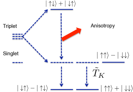
Figure S1: Low energy states of the system. One of the four states, $|\!\uparrow\downarrow\rangle+|\!\uparrow\downarrow\rangle$, is lifted due to the anisotropy of $K^{z}$ and another state, $|\!\uparrow\uparrow\rangle-|\!\downarrow\downarrow\rangle$, has higher energy due to its decoupling in Eq. (S8). The remaining doublet forms a two-dimensional low-energy space onto which we project via a Schrieffer-Wolff transformation.

At the critical $K\!=\!K_{c}(J)$ Eq. (S8) can be projected onto the Hilbert space of these two lowest energy states through a Schrieffer-Wolff transformation. First, a new set of local fermionic operators is defined,

$$d^{\dagger}d|\Omega\rangle=0\ \to\ |\Omega\rangle=(|\uparrow\uparrow\rangle+|\downarrow\downarrow\rangle)/\sqrt{2},\quad d^{\dagger}d|\Omega^{\prime}\rangle=|\Omega^{\prime}\rangle\ \to\ |\Omega^{\prime}\rangle=(|\uparrow\downarrow\rangle-|\downarrow\uparrow\rangle)/\sqrt{2}.$$ (S9)

Then, the fermionic fields are rotated by $\tilde{\psi}_{\beta}(x)\!=\!\psi_{\beta}(x)e^{-i\pi d^{\dagger}d}$ to ensure the anti-commutation relations. Projecting onto this low-energy two-dimensional subspace yields

$$H_{1}=\sum_{\beta=\left\{c,s,sf,cf,\varphi\right\}}H^{0}_{\beta}+\tilde{J}[\tilde{\psi}_{sf}(0)-\tilde{\psi}_{sf}^{\dagger}(0)](d+d^{\dagger})-(K-K_{c})d^{\dagger}d,$$ (S10)

where

$$\tilde{J}=\frac{J}{\sqrt{2\pi\alpha}}\left[1+\frac{J}{4\pi\alpha(K_{c}+{\tilde{T}}_{K})}\right].$$ (S11)

To validate the Schrieffer-Wolff transformation above, $K-K_{c}\ll\tilde{J}$ must be satisfied such that those two ground states are approximately degenerate. $\tilde{T}_{K}$ here is the Kondo temperature that results from the leads screening the doublet described by $d$ and $d^{\dagger}$. The $d^{\dagger}d$ term of Eq. (S10) is a relevant perturbation (since it breaks the degeneracy between the two states of Fig. S1). Hence, for $K\!\neq\!K_{c}$ the system is driven away from the two-impurity Kondo fixed point.

II.3 C.   The charge transport operator

All the steps that lead to Eq. (S10) now must be applied to $H_{2}\!=\!H^{0}_{\varphi}+H_{LR}$. We start by disregarding the dissipative terms. Carrying out bosonization, unitary transformation, and refermionization as in section II.1, we obtain

$$H_{LR} = V_{LR}\left\{[\psi^{\dagger}_{cf}(0)+\psi_{cf}(0)](-S_{L}^{-}S^{z}_{R}+S^{z}_{L}S^{-}_{R}-S^{+}_{L}S^{z}_{R}+S^{z}_{L}S^{+}_{R})\right.$$ (S12c)

$$+\;[\psi^{\dagger}_{cf}(0)\psi^{\dagger}_{sf}(0)-\psi^{\dagger}_{sf}(0)\psi_{cf}(0)]S^{-}_{L}S^{+}_{R}+{\rm h.c.}$$

$$+\left.[\psi_{sf}(0)-\psi^{\dagger}_{sf}(0)][\psi_{cf}(0)+\psi^{\dagger}_{cf}(0)]S^{z}_{L}S^{z}_{R}\right\}.$$

To carry out the Schrieffer-Wolff transformation, we first note how each of the local operators in this expression acts on the low energy doublet of local degrees of freedom:

$$(-S_{L}^{-}S^{z}_{R}+S^{z}_{L}S^{-}_{R}-S^{+}_{L}S^{z}_{R}+S^{z}_{L}S^{+}_{R})(|\uparrow\uparrow\rangle+|\downarrow\downarrow\rangle)/\sqrt{2}=(|\uparrow\downarrow\rangle-|\downarrow\uparrow\rangle)/\sqrt{2},$$ (S13)

$$(-S_{L}^{-}S^{z}_{R}+S^{z}_{L}S^{-}_{R}-S^{+}_{L}S^{z}_{R}+S^{z}_{L}S^{+}_{R})(|\uparrow\downarrow\rangle-|\downarrow\uparrow\rangle)/\sqrt{2}=(|\uparrow\uparrow\rangle+|\downarrow\downarrow\rangle)/\sqrt{2},$$

$$(S_{L}^{-}S_{R}^{+})(|\uparrow\uparrow\rangle+|\downarrow\downarrow\rangle)/\sqrt{2}=0,$$ (S14)

$$(S_{L}^{-}S_{R}^{+})(|\uparrow\downarrow\rangle-|\downarrow\uparrow\rangle)/\sqrt{2}=|\downarrow\uparrow\rangle/\sqrt{2},$$

$$(S_{L}^{z}S_{R}^{z})(|\uparrow\uparrow\rangle+|\downarrow\downarrow\rangle)/\sqrt{2}=\frac{(|\uparrow\uparrow\rangle+|\downarrow\downarrow\rangle)}{4\sqrt{2}},$$ (S15)

$$(S_{L}^{z}S_{R}^{z})(|\uparrow\downarrow\rangle-|\downarrow\uparrow\rangle)/\sqrt{2}=\frac{(|\uparrow\downarrow\rangle-|\downarrow\uparrow\rangle)}{4\sqrt{2}},$$

Eq. (S13) shows that the local operator appearing in Eq. (S12c), $-S_{L}^{-}S^{z}_{R}+S^{z}_{L}S^{-}_{R}-S^{+}_{L}S^{z}_{R}+S^{z}_{L}S^{+}_{R}$, acts on the doublet as $(d+d^{\dagger})$. Turning to Eq. (S12c), we see from (S14) that $S_{L}^{-}S_{R}^{+}$ is proportional to $d^{\dagger}d$. Notice that the lead operators that couple to it have scaling dimension one, and we will see that $d^{\dagger}d$ has scaling dimension 1/2 around the critical point [see the first paragraph after Eq. (7) of the main text]. Thus, the first order projection of $S_{L}^{-}S_{R}^{+}$ is RG irrelevant, and we need consider only higher order projections. One can check that

$$\hat{Q}S^{z}_{-}(1-\hat{Q})S^{-}_{L}S^{+}_{R}(1-\hat{Q})S^{x}_{+}\hat{Q}=\frac{1}{2}d^{\dagger}=\hat{Q}S^{z}_{-}(1-\hat{Q})S^{-}_{R}S^{+}_{L}(1-\hat{Q})S^{x}_{+}\hat{Q},$$ (S16)

$$\hat{Q}S^{x}_{+}(1-\hat{Q})S^{-}_{L}S^{+}_{R}(1-\hat{Q})S^{z}_{-}\hat{Q}=\frac{1}{2}d=\hat{Q}S^{x}_{+}(1-\hat{Q})S^{-}_{R}S^{+}_{L}(1-\hat{Q})S^{z}_{-}\hat{Q},$$

where $\hat{Q}$ is the projection operator onto the local doublet. In calculating the associated lead operator, one finds cancellations such that (S12c) corresponds to an operator proportional to $(d+d^{\dagger})[\psi^{\dagger}_{cf}(0)+\psi_{cf}(0)]$. Finally, the transformation of (S12c) is similar to that of (S12c), yielding a term in first-order of form $(d^{\dagger}d-1/2)$ and in second-order again $(d+d^{\dagger})[\psi^{\dagger}_{cf}(0)+\psi_{cf}(0)]$.

The last step in this derivation is to recall that $\tilde{\psi}_{\beta}(x)\!=\!\psi_{\beta}(x)e^{-i\pi d^{\dagger}d}$; this changes the operator $(d+d^{\dagger})$ to $(d-d^{\dagger})$. Thus finally, the effective low-energy Hamiltonian for charge transport between the leads is

$$\tilde{H}_{LR}=\tilde{V}_{LR}[\tilde{\psi}^{\dagger}_{cf}(0)+\tilde{\psi}_{cf}(0)](d-d^{\dagger}),$$ (S17)

where

$$\tilde{V}_{LR}=V_{LR}\left[1+\frac{J^{2}}{8(K_{c}+\tilde{T}_{k})^{2}(2\pi\alpha)^{5/2}}\right]$$ (S18)

is the renormalized tunneling strength. As a reminder, if we start with the simplified tunneling Hamiltonian $\hat{H}_{LR}$ as mentioned in the main text, we will end with an effective Hamiltonian that shares the form of Eq. (S17) but with different $\tilde{V}_{LR}$. That is why we claim that the simplified $\hat{H}_{LR}$ catches the physics around the $K=K_{c}$ critical point.

In order to introduce dissipation (in the following section), it is convenient to express the Hamiltonian in bosonic variables, so we use the bosonization identity Eq. (S3) again. The bosonic fields thus introduced are not the same as those of Section II.1 because of the Jordan-Wigner string operator used in obtaining Eq. (S17). Nevertheless, we use the same notation for these fields in order to avoid complicating the notation. Combining all the terms, we see that the Hamiltonian is

$$H= \sum_{\beta=\left\{c,s,cf,sf,\varphi\right\}}\!\!\!H^{0}_{\beta}+2i\tilde{J}\frac{F_{sf}}{\sqrt{2\pi\alpha}}\sin\left[\phi_{sf}(0)\right](d+d^{\dagger})+2\tilde{V}_{LR}\frac{F_{cf}}{\sqrt{2\pi\alpha}}\cos[\phi_{cf}(0)](d-d^{\dagger})$$ (S19)

$$\qquad\qquad-(K-K_{c})d^{\dagger}d.$$

As in the case of the $K-K_{c}$ term, the $\tilde{V}_{LR}$ term is a relevant operator that drives the system away from the two-impurity Kondo fixed point. As mentioned in previous text, $K-K_{c}$ is a small quantity such that two ground states are approximately degenerate.

II.4 D.   Introducing dissipation

The environmental noise enters through the field $\varphi$. The charge shift operator $e^{i\sqrt{2r}\varphi(0)}$ naturally couples with the lead field representing charge transfer, namely $\phi_{cf}$. Since $\varphi$ is unaffected by the transformations of the previous section, it can be introduced by replacing $\phi_{cf}$ by $\phi_{cf}+\sqrt{2r}\varphi$ in the tunneling Hamiltonian. When $r\neq 0$, we cannot apply the refermionization procedure and are thus forced to work with the bosonic Hamiltonian,

$$H= \sum_{\beta=\left\{c,s,cf,sf,\varphi\right\}}\!\!\!\!\!\!H^{0}_{\beta}+2i\tilde{J}\frac{F_{sf}}{\sqrt{2\pi\alpha}}\sin\left[\phi_{sf}(0)\right](d+d^{\dagger})+2\tilde{V}_{LR}\frac{F_{cf}}{\sqrt{2\pi\alpha}}\cos[\phi_{cf}(0)+\sqrt{2r}\varphi(0)](d-d^{\dagger})$$ (S20)

$$-(K-K_{c})d^{\dagger}d.$$

For $K\!=\!K_{c}$, this is Eq. (7) of the main text.

III III.   Conductance at the Intermediate Fixed Points

III.1 A.   Conductance at zero temperature

Conductance is naturally related to scattering states via, e.g., the Landauer-Büttiker approach Yu. V. Nazarov and Blanter (2009). Following Refs. Sela and Affleck (2009); Malecki et al. (2010, 2011), we use here the scattering states

$$\Psi_{j\sigma}(x)=\theta(x)\psi_{j\sigma}(x)+\sum_{j^{\prime}}\theta(-x)s_{jj^{\prime}}\psi_{j^{\prime}\sigma}(x),$$ (S21)

where $\theta(x)$ refers to an incoming fermionic state and $\theta(-x)$ refers to the scattered state. The $j$ and $j^{\prime}$ subscripts label the leads and allow us to write the scattering matrix

$$s=\left(\begin{array}[]{cc}\cos 2\delta&-i\sin 2\delta\\ -i\sin 2\delta&\cos 2\delta\end{array}\right),$$ (S22)

where $\delta\!=\!\frac{1}{2}\arg\Big{(}\sqrt{T_{\delta K}/T_{K}}+i\sqrt{T_{\rm noise}^{LR}/T_{K}}\;\Big{)}$ is the scattering phase shift Sela and Affleck (2009); Malecki et al. (2010, 2011). The crossover temperatures $T_{\delta K}$ and $T_{\rm noise}^{LR}$ are defined in the main text, and $T_{K}$ is the Kondo temperature associated with the bare dot-lead coupling.

At IFP₂, the phase shift is $\delta\!=\!\pi/4$. This has a strong consequence on the process that transfers two electrons simultaneously between the two leads, $\Psi^{\dagger}_{L\uparrow}\Psi^{\dagger}_{L\downarrow}\Psi_{R\uparrow}\Psi_{R\downarrow}$ Sela and Affleck (2009); Malecki et al. (2010, 2011). Using Eq. (S21), one finds that this process can be written as

$$\Psi^{\dagger}_{L,\uparrow}\Psi^{\dagger}_{L,\downarrow}\Psi_{R,\uparrow}\Psi_{R,\downarrow}(x)\theta(x)+\Psi^{\dagger}_{L,\uparrow}\Psi^{\dagger}_{L,\downarrow}\Psi_{R,\uparrow}\Psi_{R,\downarrow}(x)\theta(-x).$$ (S23)

This shows that the “incoming” state coincides exactly with the “outgoing” state. This perfect transmission implies that there is zero shot noise during this scattering process Yu. V. Nazarov and Blanter (2009), which in turn implies that charge transport processes will not be affected by dissipation Levy Yeyati et al. (2001); Safi and Saleur (2004). Thus, we expect perfect conductance at zero temperature.

III.2 B.   Low temperature conductance

Refs. (Gogolin et al., 2004; Kane and Fisher, 1992) show that the behavior of the linear conductance can be calculated by perturbation theory improved by RG. At low temperatures, the result is $G\propto T^{2(\chi-1)}$, where $\chi$ is the scaling dimension of the leading irrelevant operator.

For $r>1/2$, IFP₁ is the intermediate fixed point. The leading irrelevant operator has scaling dimension $(1+2r)/2$. Thus, near IFP₁ the temperature dependence of the conductance is $G\propto T^{2r-1}$.

For $r<1/2$, IFP₂ is the intermediate fixed point. The leading irrelevant operator is obtained by a duality transformation on the charge transport operator (Gogolin et al., 2004; Kane and Fisher, 1992). The scaling dimension of the dual operator is $2/(1+2r)$ , and therefore the conductance is $1-G\propto T^{2\frac{1-2r}{1+2r}}$ .

IV IV.   Boundary contribution to the zero temperature entropy

The boundary sine-Gordon model is given by the Hamiltonian

$$H=\int_{0}^{\infty}\frac{dx}{8\pi}\left\{(\partial_{x}\Phi)^{2}+\Pi^{2}(x)\right\}+\lambda\cos\left[\frac{\sqrt{g^{*}}}{2}\Phi(0)\right],$$ (S24)

where $g^{*}$ is known as the compactification ratio and the field $\Phi$ and $\Pi$ are periodic variables. The ground state degeneracy, $g(\Phi)$, of this model was evaluated in Refs. Wong and Affleck (1994); Oshikawa and Affleck (1997) for the two conformally invariant boundary conditions,

$$g_{D}(\Phi) = \frac{1}{\sqrt[4]{g^{*}}},$$ (S25)

$$g_{N}(\Phi) = \frac{\sqrt[4]{g^{*}}}{\sqrt{2}},$$ (S26)

where $D$ stands for Dirichlet and $N$ for Neumann. The model can be rewritten with a single chiral bosonic field by analytic continuation.

In the main text, the chiral bosonic fields $\tilde{\varphi}$, $\phi_{c}$, $\phi_{s}$ and $\phi_{sf}$ have $g^{*}\!=\!1$, whereas $\phi_{cf}$ has $g^{*}\!=\!1+2r$. The local degrees of freedom also contribute to the ground state degeneracy with $g_{\rm dots}\!=\!2$ .

We can now apply these known results to the two main fixed points discussed in the manuscript.

• IFP₁: $\phi_{sf}$ has a Neumann boundary condition, while $\tilde{\varphi}$, $\phi_{c}$, $\phi_{s}$, and $\tilde{\phi}_{cf}$ have Dirichlet boundary conditions. Hence, the total ground state degeneracy is

  $$g_{{\rm IFP}_{1}} = g(\tilde{\varphi})g(\phi_{c})g(\phi_{s})g(\tilde{\phi}_{cf})g(\phi_{sf})g_{\rm dots}$$ (S27)

  $$= \sqrt[4]{\frac{4}{1+2r}}\;.$$

• IFP₂: $\phi_{sf}$ and $\tilde{\phi}_{cf}$ have Neumann boundary condition, while $\tilde{\varphi}$, $\phi_{c}$, and $\phi_{s}$ have Dirichlet boundary condition. The total ground state degeneracy for this case is

$$g_{{\rm IFP}_{2}} = \sqrt[4]{1+2r}\;.$$ (S28)

References

- Mebrahtu et al. (2012) H. T. Mebrahtu, I. V. Borzenets, Dong E. Liu, Huaixiu Zheng, Yu. V. Bomze, A. I. Smirnov, H. U. Baranger, and G. Finkelstein, “Quantum phase transition in a resonant level coupled to interacting leads,” Nature 488, 61–64 (2012).
- Mebrahtu et al. (2013) H. T. Mebrahtu, I. V. Borzenets, H. Zheng, Yu. V. Bomze, A. I. Smirnov, S. Florens, H. U. Baranger, and G. Finkelstein, “Observation of Majorana quantum critical behavior in a resonant level coupled to a dissipative environment,” Nat. Phys. 9, 732–737 (2013), arXiv:1212.3857.
- Hewson (1993) A. C. Hewson, The Kondo Problem to Heavy Fermions (Cambridge University Press, New York, 1993).
- Jayatilaka et al. (2011) F. W. Jayatilaka, M. R. Galpin, and D. E. Logan, “Two-channel Kondo physics in tunnel-coupled double quantum dots,” Phys. Rev. B 84, 115111 (2011).
- Gan (1995) Junwu Gan, “Solution of the two-impurity Kondo model: Critical point, Fermi-liquid phase, and crossover,” Phys. Rev. B 51, 8287–8309 (1995).
- Gogolin et al. (2004) A. O. Gogolin, A. A. Nersesyan, and A. M. Tsvelik, Bosonization and Strongly Correlated Systems (Cambridge University Press, Cambridge, 2004).
- Yu. V. Nazarov and Blanter (2009) Yu. V. Nazarov and Y. M. Blanter, Quantum Transport: Introduction to Nanoscience (Cambridge University Press, Cambridge, 2009).
- Sela and Affleck (2009) E. Sela and I. Affleck, “Resonant pair tunneling in double quantum dots,” Phys. Rev. Lett. 103, 087204 (2009).
- Malecki et al. (2010) J. Malecki, E. Sela, and I. Affleck, “Prospect for observing the quantum critical point in double quantum dot systems,” Phys. Rev. B 82, 205327 (2010).
- Malecki et al. (2011) J. Malecki, E. Sela, and I. Affleck, “Erratum: Prospect for observing the quantum critical point in double quantum dot systems [Phys. Rev. B 82, 205327 (2010)],” Phys. Rev. B 84, 159907(E) (2011).
- Levy Yeyati et al. (2001) A. Levy Yeyati, A. Martin-Rodero, D. Estève, and C. Urbina, “Direct link between Coulomb blockade and shot noise in a quantum-coherent structure,” Phys. Rev. Lett. 87, 046802 (2001).
- Safi and Saleur (2004) I. Safi and H. Saleur, “One-channel conductor in an Ohmic environment: Mapping to a Tomonaga-Luttinger liquid and full counting statistics,” Phys. Rev. Lett. 93, 126602 (2004).
- Kane and Fisher (1992) C. L. Kane and M. P. A. Fisher, “Transmission through barriers and resonant tunneling in an interacting one-dimensional electron gas,” Phys. Rev. B 46, 15233–15262 (1992).
- Wong and Affleck (1994) E. Wong and I. Affleck, “Tunneling in quantum wires: A boundary conformal field theory approach,” Nucl. Phys. B 417, 403–438 (1994).
- Oshikawa and Affleck (1997) M. Oshikawa and I. Affleck, “Boundary conformal field theory approach to the critical two-dimensional Ising model with a defect line,” Nucl. Phys. B 495, 533–582 (1997).
- Note (1) Ref.\tmspace+.1667emGogolin et al. (2004) p. 397.