Equilibrium and Sudden Events in Chemical Evolution

Abstract

We present new analytic solutions for one-zone (fully mixed) chemical evolution models and explore their implications. In contrast to existing analytic models, we incorporate a realistic delay time distribution for Type Ia supernovae (SNIa) and can therefore track the separate evolution of $\alpha$-elements produced by core collapse supernovae (CCSNe) and iron peak elements synthesized in both CCSNe and SNIa. Our solutions allow constant, exponential, or linear-exponential ($te^{-t/\tau_{\rm sfh}}$) star formation histories, or combinations thereof. In generic cases, $\alpha$ and iron abundances evolve to an equilibrium at which element production is balanced by metal consumption and gas dilution, instead of continuing to increase over time. The equilibrium absolute abundances depend principally on supernova yields and the outflow mass loading parameter $\eta$, while the equilibrium abundance ratio $[\alpha/{\rm Fe}]$ depends mainly on yields and secondarily on star formation history. A stellar population can be metal-poor either because it has not yet evolved to equilibrium or because high outflow efficiency makes the equilibrium abundance itself low. Systems with ongoing gas accretion develop metallicity distribution functions (MDFs) that are sharply peaked, while “gas starved” systems with rapidly declining star formation, such as the conventional “closed box” model, have broadly peaked MDFs. A burst of star formation that consumes a significant fraction of a system’s available gas and retains its metals can temporarily boost $[\alpha/{\rm Fe}]$ by 0.1-0.3 dex, a possible origin for rare, $\alpha$-enhanced stars with intermediate age and/or high metallicity. Other sudden transitions in system properties can produce surprising behavior, including backward evolution of a stellar population from high metallicity to low metallicity. While one-zone models omit mixing processes that may play an important role in chemical evolution, they provide a useful guide and flexible tool for interpreting multi-element surveys of the Milky Way and its neighbors. An Appendix provides a user’s guide for calculating enrichment histories, $[\alpha/{\rm Fe}]$ tracks, and MDFs in a wide variety of scenarios.

1. Introduction

The elemental abundances of stars provide essential clues to the star formation and assembly history of the Milky Way and other galaxies. One of the most useful “clocks” for tracing these histories is the ratio of $\alpha$-elements, which are produced in massive, short-lived stars that explode as core collapse supernovae (CCSNe), to iron peak elements, which are produced by both CCSNe and Type Ia supernovae (SNIa). Old metal-poor stars in the stellar halo and thick disk have enhanced $[\alpha/{\rm Fe}]$, while disk stars with near-solar iron abundance ($[{\rm Fe}/{\rm H}]\approx 0$) typically have solar abundance ratios as well ($[\alpha/{\rm Fe}]\approx 0$). A standard theoretical account might be that the enhanced $[\alpha/{\rm Fe}]$ characteristic of CCSN yields is driven towards solar $[\alpha/{\rm Fe}]$ as SNIa iron enrichment becomes important, and thereafter the iron abundance increases at fixed $[\alpha/{\rm Fe}]$ because of continuing enrichment from both classes of supernovae. However, the behavior of simple one-zone chemical evolution models is rather different: by the time that $[\alpha/{\rm Fe}]$ approaches zero, the iron abundance $[{\rm Fe}/{\rm H}]$ has also approached an approximate “equilibrium” value in which new enrichment is balanced by dilution and depletion of existing metals, so that a given model produces only a narrow range of $[{\rm Fe}/{\rm H}]$ when $[\alpha/{\rm Fe}]\approx 0$ (B. Andrews et al. 2016, in preparation, hereafter AWSJ).

This paper focuses on the phenomenon of equilibrium abundances and on the departures from equilibrium that can arise from bursts of star formation or other sudden changes. Over the past decade, theoretical discussions of the “mass-metallicity” relation — the correlation between the stellar mass and gas-phase oxygen abundance of galaxies — have concluded that the oxygen abundance of a galaxy’s interstellar medium (ISM) is controlled by an equilibrium among fresh gas accretion, star formation, and outflows (e.g., Dalcanton 2007; Finlator & Davé 2008; Peeples & Shankar 2011; Lilly et al. 2013). This account has early roots in the work of Larson (1972), who shows that, in the instantaneous recycling approximation, ISM abundances in a galaxy with continuous infall approach an equilibrium determined by nucleosynthetic yields.

It is less obvious that equilibrium is a useful concept for describing iron abundances, since SNIa provide enrichment over long timescales not tied to the current star formation rate. However, observational studies of the evolution of the SNIa rate and the relative rates in star-forming and passive galaxies now indicate that a large fraction of SNIa explode within 1-3 Gyr of the birth of their stellar progenitors (Scannapieco & Bildsten, 2005; Maoz & Mannucci, 2012; Maoz et al., 2012), in agreement with predictions of binary population synthesis models (Greggio, 2005). The dominance of relatively “prompt” SNIa makes equilibrium approximations relevant even for iron abundances, though the different timescale of CCSN and SNIa enrichment remains crucial to understanding the evolution of abundance ratios.

Our discussion relies mainly on analytic approximations, though we test their results against numerical calculations that avoid the simplifying assumptions needed for analytic solutions. Relative to existing analytic models of chemical evolution, the distinctive feature of our approach is that we do not assume instantaneous recycling for SNIa enrichment but instead adopt an exponential form for the delay time distribution that allows analytic solutions of the resulting differential equations for interesting families of star formation histories. We do assume instantaneous recycling for CCSN enrichment and for the return of envelope material from evolved stars, but incorporating realistic time evolution for SNIa allows us to calculate evolution in the $[\alpha/{\rm Fe}]-[{\rm Fe}/{\rm H}]$ plane and to make more realistic calculations of $[{\rm Fe}/{\rm H}]$ evolution and metallicity distribution functions. Our choices of parameters for our calculations are largely guided by the discussion of AWSJ, who examine a broader range of models and a broader range of chemical evolution results. For definiteness, we focus on oxygen as our representative $\alpha$ element, but our results translate trivially to other elements whose production is dominated by CCSNe.

The phenomena discussed here are necessarily incorporated into most existing numerical chemical evolution models, as they have similar physical ingredients. However, the analytic discussion and the focus on equilibrium provide physical insights into the behavior of these models, and they suggest new ways to think about phenomena now being revealed by large scale Galactic chemical evolution studies. As surveys like SEGUE (Yanny et al., 2009), APOGEE (Majewski et al., 2016), Gaia-ESO (Gilmore et al., 2012), and GALAH (De Silva et al., 2015) extend measurements of $\alpha$ and iron abundances over much of the Milky Way, flexible models that allow rapid explorations of a large parameter space are a useful tool for developing interpretations. They are also useful for modeling the stellar populations of other galaxies and the relation of those populations to gas phase abundances, and potentially for population synthesis modeling of galaxy spectra. Radial mixing of stellar populations and radial flows of enriched gas are both likely to play important roles in the chemical evolution of disk galaxies like the Milky Way (e.g., Schönrich & Binney 2009; Bilitewski & Schönrich 2012; Pezzulli & Fraternali 2016), and both processes violate the assumptions of one-zone models in which metals produced by stars are either ejected from the system or retained locally. However, fully understanding the behavior of one-zone models is important for evaluating the empirical case for mixing processes, and mixtures of one-zone models may provide a useful approximate description of more complex scenarios.

Section 2.1 gives a brief high-level overview of our models in the broader context of chemical evolution calculations. Section 2.2 introduces our basic notation and evolution equations for oxygen and iron mass, and §§2.3 and 2.4 show how these equations lead to equilibrium abundances for constant or exponentially declining star formation histories. Section 3 derives the full time evolution solutions for these cases and for linear-exponential star formation histories, then discusses metallicity distribution functions and the relation of our calculations to traditional analytic models of chemical evolution. This section concludes with illustrations of behavior for a variety of model parameters and tests against numerical solutions. Section 4 considers the impact of an instantaneous burst of star formation on abundances and abundance ratios, then shows how to stitch together our previous analytic solutions for cases where model parameters change suddenly from one set of values to another. These cases allow an interesting variety of behaviors. Section 5 considers a variety of extensions of our results, including more complex time histories of SNIa or star formation, metal-enriched infall, and elements that have both CCSN and SNIa contributions. Section 6 summarizes many of the insights from our results in qualitative terms. Some readers may prefer to start with the illustrations in §3.6, jump to the qualitative conclusions in §6, then go back as needed to the analytic modeling that leads to them. Tables 1 and 2 provide a guide to the notation used in the paper and the sections where the principal analytic results appear. Appendix B provides a guide for readers who want to use our results to compute enrichment histories, $[\alpha/{\rm Fe}]-[{\rm Fe}/{\rm H}]$ tracks, and distribution functions of metallicity or abundance ratios.

2. Equilibrium Abundances

2.1. Context

Before diving into notation and equations, it is useful to place our calculations in the broader context of chemical evolution models. Classic reviews of the subject include Tinsley (1980) and the monographs of Pagel (1997) and Matteucci (2001, 2012). Key elements of any chemical evolution model include a gas accretion history, a star formation law, an outflow prescription, and nucleosynthetic yields as a function of time. In one-zone models (Schmidt, 1959, 1963), abundances in the gas phase are assumed to be homogeneous throughout the model volume, and all stars form with the current abundances of the ISM. In our models we generally assume that the star formation rate is proportional to the gas mass, with the star formation efficiency as a free but constant parameter. This assumption, sometimes referred to in the literature as a “linear Schmidt law” (e.g., Recchi et al. 2008), is arguably the least desirable requirement of our solutions, since observations imply that the star formation efficiency declines with decreasing total (atomic + molecular) gas surface density (Schmidt, 1959; Kennicutt, 1998). As in most models, we assume that the gas outflow rate is a constant multiple of the star formation rate, specified by a mass loading parameter. We explicitly specify a model’s star formation history, which may be constant, exponentially declining, or the product of a linear rise and an exponential decline. With these assumptions, the gas accretion history follows implicitly from the star formation history once the star formation efficiency and mass loading are specified (see eq. 9 below). This choice to define the functional form of the star formation rate rather than the gas accretion rate differs from most models, but if the star formation rate is simply related to the gas supply then these two histories usually track each other fairly closely.

Nearly all analytic models of chemical evolution rely on the instantaneous recycling approximation, that the elements synthesized by newly formed stars are immediately returned and mixed into the star-forming ISM. We adopt this approximation for elements produced by CCSNe, which come from stars with $M>8M_{\odot}$ and lifetimes less than 40 Myr. The key insight that underlies much of this paper is that analytic solutions for SNIa enrichment are possible if the delay time distribution (DTD) is assumed to be an exponential in time (following a minimum delay), or a sum of exponentials. Even for CCSN products, instantaneous recycling may be a poor approximation if the metals in SN ejecta are locked up in a warm or hot phase of the ISM and return only slowly to the cold, star-forming phase (see, e.g., Schönrich & Binney 2009). We ignore this possibility here, though we note that our solutions could be easily adapted to this case if one assumed an exponential form for this gas return. Likewise, our DTD for SNIa enrichment should be understood as representing the time for SNIa products to return to the star-forming phase of the ISM, which may differ from the time for the SNIa explosions themselves. Our analytic solutions require assuming that nucleosynthetic yields are independent of stellar metallicity. With the yield sources adopted by AWSJ (and described below), metallicity independence is a good approximation for oxygen and other $\alpha$-elements, and for iron. However, the supernova yields are uncertain, and population averaged yields could in any case become metallicity dependent if the mass ranges of stars that explode as CCSNe changes with metallicity.

Our standard solutions apply to models with parameters that remain fixed throughout the time evolution, and that have the smooth star formation histories described above. However, in §4 we show how to combine solutions to create models with a sharp transition in accretion history. The most well known example of a (numerical) chemical evolution model with a sharp transition in accretion history is the “two infall” scenario of Chiappini et al. (1997), which posits distinct infall episodes for the formation of the Milky Way’s halo-thick disk and thin disk, respectively. Some numerical models incorporate accretion histories motivated by cosmological simulations Colavitti et al. (2008), which typically transition from rapid to slow accretion, somewhat analogous to the two infall model.

Models of disk galaxies are frequently built as a sequence of annular zones, each of which evolves independently with its own gas accretion history (e.g., Matteucci & Francois 1989). Such a model could be created as a sequence of our solutions, with parameters that depend on Galactocentric radius. However, there are processes that can redistribute stars and metals from one annulus to another. One of these is radial mixing of stars (Sellwood & Binney, 2002; Roškar et al., 2008; Bird et al., 2012), which is invoked to explain the observed dispersion between metallicity and stellar age (Edvardsson et al., 1993; Wielen et al., 1996) and could have a large impact on metallicity gradients and distribution functions (Schönrich & Binney, 2009). These effects can be modeled crudely by after-the-fact convolutions of a simple annular-zone model (e.g., Hayden et al. 2015). A second mixing process arises because gas accreted from the halo should have angular momentum below that of local circular orbits in the disk (Fraternali & Binney, 2008), driving radial flows that carry metals inward from the radius at which they are produced. Numerical and analytic models that include such radial gas flows are discussed by Spitoni & Matteucci (2011), Bilitewski & Schönrich (2012) and Pezzulli & Fraternali (2016). Large scale galactic winds could provide a third redistribution mechanism that carries metals from small radii to large radii, if some enriched gas is not ejected entirely from the halo but instead returns as a galactic fountain. We provide solutions with enriched infall of constant metallicity (§5.2), but we do not address this more general case.

2.2. Evolution equations

Our analytic models of chemical evolution assume that the star-forming ISM is always fully mixed, that CCSNe and SNIa are the only sources of new metal production, and that CCSNe redistribute their metals to the ISM instantaneously. AGB stars are a source of some heavy elements, most notably nitrogen and $s$-process neutron capture elements, but they make a negligible contribution to the production of oxygen and other $\alpha$-elements. They do return the metals they were born with, however, and to enable analytic solutions we assume that this return of birth-metals happens instantaneously. For the delay time distribution (DTD) of SNIa, we will usually assume an exponential form (Schönrich & Binney, 2009) with a minimum delay time $t_{D}$,

$$R(t)=\begin{cases}R_{0}e^{-(t-t_{D})/\tau_{\rm Ia}}&t\geq t_{D}~{},\\ 0&t<t_{D}~{},\end{cases}$$ (1)

which proves analytically convenient. Here $R(t)dt$ is the number of SNIa in the time interval $t\rightarrow t+dt$ per unit mass of stars formed at time $t=0$; $R_{0}$ has units of $M_{\odot}^{-1}\,{\rm yr}^{-1}$. With $\tau_{\rm Ia}=1.5\,{\rm Gyr}$, equation (1) roughly tracks the predictions of population synthesis models (Greggio 2005; see Fig. 6 of AWSJ for a comparison). As discussed in §5.1, our analytic results generalize easily to a DTD that is a sum of exponentials, which can be used to approximate other forms such as a power-law DTD (Maoz & Mannucci, 2012; Maoz et al., 2012). Note that population synthesis models and supernova statistics both address the DTD for supernova explosions, but what matters for chemical evolution is the time for SNIa elements to return to the star-forming ISM, which may be longer if the supernova ejecta are initially deposited in a warm or hot phase.

We define the dimensionless yield parameters:

• $m_{\rm O}^{\rm cc}$, the mass of newly produced oxgyen returned to the ISM by CCSNe per unit mass of star formation,

• $m_{\rm Fe}^{\rm cc}$, the mass of newly produced iron returned to the ISM by CCSNe per unit mass of star formation, and

• $m_{\rm Fe}^{\rm Ia}$, mass of newly produced iron returned to the ISM by SNIa per unit mass of star formation.

With the fiducial model assumptions of AWSJ, a Kroupa (2001) initial mass function (IMF) and the CCSN yields of Chieffi & Limongi (2004) and Limongi & Chieffi (2006), the core collapse quantities are $m_{\rm O}^{\rm cc}=0.015$ and $m_{\rm Fe}^{\rm cc}=0.0012$: for every $100M_{\odot}$ of star formation with a Kroupa IMF (truncated outside $0.1-100M_{\odot}$), CCSNe produce an average of $1.5M_{\odot}$ of oxygen and $0.12M_{\odot}$ of iron. (These numbers are slightly metallicity-dependent, and our values here are for $Z\approx 0.1Z_{\odot}$.) If the average mass of iron from an individual SNIa is $K_{\rm Fe}^{\rm Ia}$, then

$$m_{\rm Fe}^{\rm Ia}\equiv K_{\rm Fe}^{\rm Ia}\int_{0}^{\infty}R(t)dt=K_{\rm Fe}^{\rm Ia}R_{0}\tau_{\rm Ia},$$ (2)

where the second equality holds for an exponential DTD. (The notation $K_{\rm Fe}^{\rm Ia}$ is chosen here only to reduce confusion with variables used elsewhere in the paper.) For the AWSJ fiducial model, with $R_{0}=2.2\times 10^{-3}M_{\odot}^{-1}\,\,{\rm yr}^{-1}$ (based on Maoz & Mannucci 2012) and $K_{\rm Fe}^{\rm Ia}=0.77M_{\odot}$ (based on the W70 model of Iwamoto et al. 1999), the time-integrated yield is $m_{\rm Fe}^{\rm Ia}=0.0017$. Note that one can think of $m_{\rm O}^{\rm cc}$, $m_{\rm Fe}^{\rm cc}$, and $m_{\rm Fe}^{\rm Ia}$ as having units of “solar masses per solar mass.”

We define

• $\eta=\dot{M}_{\rm outflow}/\dot{M}_{*}$, the mass loading factor, to be the ratio of gas mass ejected from the ISM by stellar feedback to the gas mass being incorporated into stars, and

• $r$, the recycling parameter, to be the fraction of mass formed into stars that is returned from the envelopes of CCSN progenitors and asymptotic giant branch (AGB) stars at its original metallicity.

In most theoretical models of galaxy formation and chemical evolution, reproducing the observed stellar masses and metallicities of galaxies requires substantial outflows, with time-averaged mass loading factors $\eta\approx 1-10$. The characteristic value of $\eta$ likely varies with galaxy mass and evolutionary state, and in any given galaxy it may vary with time and location. For a Kroupa IMF, the recycled fraction is $r(t)=0.37$, 0.40, and 0.45 after 1, 2, and 10 Gyr, respectively. The quantities $m_{\rm O}^{\rm cc}$ and $m_{\rm Fe}^{\rm cc}$ refer to the “net yields” of CCSNe, while the “absolute yields” include the recycling of the progenitor’s original metals, which is encompassed here under $r$. For our analytic solutions we must assume instantaneous recycling and a single value of $r$, and we adopt $r=0.4$ for a Kroupa IMF based on comparing our analytic results to those of numerical calculations that include time-dependent recycling (see §3.7). While the timescale for envelope return from AGB stars is comparable to the delay timescales for SNIa, the supernovae are a primary source of new iron while the AGB stars are merely returning the metals they were born with, so it is useful to have full time evolution of SNIa even if the AGB return is approximated as instantaneous.

We define the characteristic timescales

• $\tau_{*}=M_{g}/\dot{M}_{*}$, the star formation efficiency (SFE) timescale, to be the ratio of the current ISM gas mass $M_{g}$ to the instantaneous star formation rate $\dot{M}_{*}$, and

• $\tau_{\rm dep}=\tau_{*}/(1+\eta-r)$, the gas depletion timescale, to be the net rate at which gas is being depleted by the combination of star formation and outflows.

The SFE timescale is more observationally accessible than the gas depletion timescale because $\eta$ is usually difficult to determine. The observations of Leroy et al. (2008) suggest a typical $\tau_{*}\approx 2\,{\rm Gyr}$ for the molecular ISM, over a wide range of star formation rate and gas surface density, though the corresponding timescale for the molecular+atomic ISM will be longer. With our instantaneous approximation, CCSNe and AGB stars return mass to the ISM at a rate $r\dot{M}_{*}$, making the net depletion timescale $\tau_{*}/(1+\eta-r)$ rather than $\tau_{*}/(1+\eta)$. We note that terminology in the literature is not universal, and that some papers define the gas depletion timescale (or gas consumption timescale) to be the quantity we call $\tau_{*}$, rather than what we call $\tau_{\rm dep}$. Note also that because of recycling, the mass in stars and stellar remnants at a given time is

$$M_{*}(t)=(1-r)\int_{0}^{t}\dot{M}_{*}(t^{\prime})dt^{\prime}~{}.$$ (3)

With these definitions and assumptions, the injection rate of oxygen mass and iron mass into the ISM is

$$\dot{M}_{\rm O,in} = m_{\rm O}^{\rm cc}\dot{M}_{*}+rZ_{\rm O}\dot{M}_{*}~{},$$ (4)

$$\dot{M}_{\rm Fe,in} = m_{\rm Fe}^{\rm cc}\dot{M}_{*}+m_{\rm Fe}^{\rm Ia}\langle\dot{M}_{*}\rangle_{\rm Ia}+rZ_{\rm Fe}\dot{M}_{*}~{},$$ (5)

where $Z_{\rm O}=M_{\rm O}/M_{g}$ and $Z_{\rm Fe}=M_{\rm Fe}/M_{g}$ are the mass-weighted oxygen and iron abundances of the ISM and $\langle\dot{M}_{*}\rangle_{\rm Ia}$ is the time-averaged star formation rate (SFR) weighted by the SNIa rate. Specifically, as shown in Appendix A

$$\langle\dot{M}_{*}(t)\rangle_{\rm Ia}\equiv{\int_{0}^{t}\dot{M}_{*}(t^{\prime})R(t-t^{\prime})dt^{\prime}\over\int_{0}^{\infty}R(t^{\prime})dt^{\prime}}~{}.$$ (6)

To compute the full time derivatives of oxygen and iron mass, we must also take account of the consumption of ISM metals by star formation and outflow, obtaining:

$$\dot{M}_{\rm O} = m_{\rm O}^{\rm cc}\dot{M}_{*}-(1+\eta-r)\dot{M}_{*}Z_{\rm O}~{},$$ (7)

$$\dot{M}_{\rm Fe} = m_{\rm Fe}^{\rm cc}\dot{M}_{*}+m_{\rm Fe}^{\rm Ia}\langle\dot{M}_{*}\rangle_{\rm Ia}-(1+\eta-r)\dot{M}_{*}Z_{\rm Fe}~{}.$$ (8)

By approximating recycling as instantaneous, and occurring at the current abundance $Z_{\rm O}$ or $Z_{\rm Fe}$, we are able to include it by simply using $1+\eta-r$ instead of $1+\eta$ in these equations. In physical terms, the impact of recycling is the same as replacing $\eta$ with an “effective” value $\eta-r$ (which may be negative) because some gas and metals are immediately returned to the system. With full time-dependent AGB recycling there would be a source term that depends on the metallicity at earlier times, leading to integro-differential equations that would defy analytic solution except in special circumstances.

The evolution of $M_{g}(t)$ is specified implicitly in our models through a star formation history and the SFE timescale, with $M_{g}(t)=\tau_{*}\dot{M}_{*}(t)$. This in turn determines the rate at which abundances are diluted by gas infall. The time derivative of the gas supply is $\dot{M}_{g}=-(1+\eta-r)\dot{M}_{*}+\dot{M}_{\rm inf}$, where $\dot{M}_{\rm inf}$ is the infall rate. For constant $\tau_{*}$, we can set $\dot{M}_{g}=\tau_{*}\ddot{M}_{*}$ to obtain

$$\dot{M}_{\rm inf}=(1+\eta-r)\dot{M}_{*}+\tau_{*}\ddot{M}_{*}~{}.$$ (9)

Our approximation of instantaneous recycling for CCSN products implicitly assumes that the CCSN elements that are not ejected in outflow become immediately available for star formation from the cold ISM. It is possible that CCSN products are instead injected into a warm phase of the ISM and cool over time to join the star-forming medium, as in, for example, the Schönrich & Binney (2009) chemical evolution model. We ignore this complication here, but we note that one could accommodate this scenario within our analytic framework if the return of CCSN elements were approximated as exponential in time (or a sum of exponentials), perhaps with a minimum delay. In this case, one would simply adapt our solutions for $M_{\rm Fe}^{\rm Ia}$ and $Z_{\rm Fe}^{\rm Ia}$ to CCSN elements with the appropriate $e-$folding and minimum delay timescales. Similarly, one could incorporate time-dependent production of AGB elements by approximating AGB enrichment as a delayed exponential.

Variable	Description	Section	Fiducial Value
$\eta$	$=\dot{M}_{\rm outflow}/\dot{M}_{*}$, outflow efficiency	§2.2	2.5
$\eta_{0}$	starting value of $\eta$ with time-dependent $\tau_{*}$	§5.5
$f_{*}$	fraction of gas converted to stars in burst	§4.1
$f_{g}$	$=M_{g}(t)/M_{i}$, gas fraction in closed/leaky box model	§3.5
$f_{\rm met}$	fraction of newly produced metals retained in burst	§4.1
$F_{\rm unp}$	fraction of gas unprocessed in burst	§4.1
$K_{\rm Fe}^{\rm Ia}$	iron mass yield per SNIa	§2.2	$0.77M_{\odot}$
$m_{\rm O}^{\rm cc}$	IMF-integrated CCSN oxygen yield	§2.2	0.015
$m_{\rm Fe}^{\rm cc}$	IMF-integrated CCSN iron yield	§2.2	0.0012
$m_{\rm Fe}^{\rm Ia}$	IMF-integrated SNIa iron yield	§2.2	0.0017
$M_{g}$	gas mass	§2.2
$M_{\rm O}$	oxygen mass	§2.2
$M_{\rm Fe}$	total iron mass	§2.2
$M_{\rm Fe}^{\rm Ia}$	iron mass from SNIa alone	§2.2
$\dot{M}_{*}$	star-formation rate	§2.2
$M_{*}$	mass of stars + stellar remnants	§2.2
$M_{\rm form}(t)$	$=\int_{0}^{t}\dot{M}_{*}(t^{\prime})dt^{\prime}=M_{*}(t)/(1-r)$	§5.3
$\langle\dot{M}_{*}\rangle_{\rm Ia}$	SFR averaged over SNIa DTD	§2.2
$\dot{M}_{\rm inf}$	infall rate	§2.2
$R(t)$	SNIa rate from population formed at $t=0$	§2.2
$r$	mass recycling parameter (CCSN + AGB)	§2.2	0.4
$r_{\rm cc}$	mass recycling parameter (CCSN only)	§4.1	0.2
$\tau_{*}$	$=M_{g}/\dot{M}_{*}$, star formation efficiency (SFE) timescale	§2.2	1 Gyr
$\tau_{*,0}$	starting value of $\tau_{*}$ with time-dependent $\tau_{*}$	§5.5
$\tau_{\rm dep}$	$=\tau_{*}/(1+\eta-r)$, gas depletion timescale	§2.2	0.323 Gyr
$\tau_{\rm dep,0}$	starting value of $\tau_{\rm dep}$ with time-dependent $\tau_{*}$	§5.5
$\tau_{\rm Ia}$	$e$-folding timescale of SNIa DTD	§2.2	1.5 Gyr
$t_{D}$	minimum delay time for SNIa	§2.2	0.15 Gyr
$\Delta t$	$=t-t_{D}$, shifted time variable	§2.3
$t_{c}$	transition time in sudden-change models	§4.2
$\tau_{\rm sfh}$	star formation history timescale, $\dot{M}_{*}\propto e^{-t/\tau_{\rm sfh}}$	§2.4	6 Gyr
$\bar{\tau}_{[X,Y]}$	$=1/(\tau_{X}^{-1}-\tau_{Y}^{-1})$, harmonic difference timescale	§2.4
$\bar{\tau}_{[{\rm Ia,sfh}]}$	$=1/(\tau_{\rm Ia}^{-1}-\tau_{\rm sfh}^{-1})$	§2.4	2 Gyr
$\bar{\tau}_{[{\rm dep,sfh}]}$	$=1/(\tau_{\rm dep}^{-1}-\tau_{\rm sfh}^{-1})$	§2.4	0.341 Gyr
$\bar{\tau}_{[{\rm dep,Ia}]}$	$=1/(\tau_{\rm dep}^{-1}-\tau_{\rm Ia}^{-1})$	§3.1	0.412 Gyr
$Z_{\rm O}$	$=M_{\rm O}/M_{g}$, oxygen abundance	§2.2
$Z_{\rm Fe}$	$=M_{\rm Fe}/M_{g}$, iron abundance	§2.2
$Z_{\rm Fe}^{\rm cc}$	$=M_{\rm Fe}^{\rm cc}/M_{g}$, CCSN iron abundance	§3.1
$Z_{\rm Fe}^{\rm Ia}$	$=M_{\rm Fe}^{\rm Ia}/M_{g}$, SNIa iron abundance	§3.1
$Z_{\rm O,eq}$	equilibrium oxygen abundance	§2.4	0.51%
$Z^{\rm cc}_{\rm Fe,eq}$	equilibrium CCSN iron abundance	§2.4	0.041%
$Z^{\rm Ia}_{\rm Fe,eq}$	equilibrium SNIa iron abundance	§2.4	0.079%
$Z_{\rm O,eqc}$	equilibrium oxygen abundance for constant SFR	§2.3
$Z_{\rm Fe,eqc}$	equilibrium iron abundance for constant SFR	§2.3
$Z_{\rm O,inf}$	oxygen abundance of enriched infall	§5.2
$Z_{\rm Fe,inf}$	iron abundance of enriched infall	§5.2
$Z_{{\rm O},\odot}$	solar oxygen abundance by mass	§3.1	0.56%
$Z_{{\rm Fe},\odot}$	solar iron abundance by mass	§3.1	0.12%
$z_{O}$	$=Z_{\rm O}/Z_{\rm O,eq}$, scaled oxygen abundance	§3.4

Table 1Variables used in the paper

Result	Location
Equilibrium abundances	§2.4, eqs. 15, 18, 27 (or eqs. 28–30)
Evolution of simple models:
Constant SFR	§3.1, eqs. 34, 35, 37
Exponential SFH	§3.2, eqs. 50, 52, 53
Lin-Exp SFH	§3.3, eqs. 56, 57, 58
Metallicity distribution functions	§3.4, eqs. 62–63
Impact of a star formation burst	§4.1, eqs. 74–76, 78, Fig. 8
Models with sudden parameter changes	§4.2, Fig. 9
Two-exponential SNIa DTD	§5.1
Enriched infall	§5.2
Stellar vs. ISM oxygen abundance	§5.3, eq. 106
Evolution of $[{\rm X}/{\rm Fe}]$	§5.4, eq. 109
Complex SFH	§5.6, eq. 117

Table 2Principal Analytic Results

2.3. Constant SFR

First consider the case of a constant $\dot{M}_{*}$, for which (see Appendix A)

$$\langle\dot{M}_{*}\rangle_{\rm Ia}=\dot{M}_{*}\left[1-e^{-(t-t_{D})/\tau_{\rm Ia}}\right]$$ (10)

at times $t\geq t_{D}$ and $\langle\dot{M}_{*}\rangle_{\rm Ia}=0$ for $t<t_{D}$. Also assume that the mass loading factor $\eta$ and SFE timescale $\tau_{*}$ are themselves not changing in time. In this case, a constant SFR corresponds to constant $M_{g}=\tau_{*}\dot{M}_{*}$, requiring that accretion and recycling from evolved stars balance the rate at which the ISM loses mass to star formation and outflow. For $t-t_{D}>\tau_{\rm Ia}$, $\langle\dot{M}_{*}\rangle_{\rm Ia}\approx\dot{M}_{*}$, and the abundance ratios can approach an equilibrium in which $\dot{M}_{\rm O}=\dot{M}_{\rm Fe}=0$. Solving equations (7)-(8) with this condition implies

$$Z_{\rm O,eqc} = m_{\rm O}^{\rm cc}/(1+\eta-r)$$ (11)

$$Z_{\rm Fe,eqc} = (m_{\rm Fe}^{\rm cc}+m_{\rm Fe}^{\rm Ia})/(1+\eta-r)~{},$$ (12)

where the “eqc” subscript denotes equilibrium for a constant star formation rate. As discussed in §3.1, the timescale to approach the equilibrium oxygen abundance is $\tau_{\rm dep}$, while the timescale to approach the equilibrium iron abundance depends on both $\tau_{\rm dep}$ and $\tau_{\rm Ia}$. The equilibrium abundances depend on the nucleosynthetic yields and the outflow rate, but they are independent of the gas depletion timescale. Furthermore, the equilibrium abundance ratio

$${Z_{\rm O,eqc}\over Z_{\rm Fe,eqc}}={m_{\rm O}^{\rm cc}\over m_{\rm Fe}^{\rm cc}+m_{\rm Fe}^{\rm Ia}},\quad\hbox{constant SFR},$$ (13)

is independent of the outflow rate.

2.4. Exponentially declining SFR

Next consider a case in which $\tau_{*}$ and $\eta$ are constant but $\dot{M}_{*}=M_{g}/\tau_{*}$ declines exponentially on a timescale $\tau_{\rm sfh}$ because accretion and recycling of gas does not keep pace with depletion of gas by star formation and outflow. (Note the distinction between $\tau_{*}$ and $\tau_{\rm sfh}$, where the latter refers to the exponential decline of the star formation history.) It is useful to rewrite equation (7) in the form

$$\dot{M}_{\rm O}=m_{\rm O}^{\rm cc}{M_{g}\over\tau_{*}}-(1+\eta-r)\left({M_{g}\over\tau_{*}}\right)\left({M_{\rm O}\over M_{g}}\right)~{}.$$ (14)

The equilibrium oxygen abundance corresponds to constant $M_{\rm O}/M_{g}$ and thus $\dot{M}_{\rm O}/M_{\rm O}=\dot{M}_{g}/M_{g}=-1/\tau_{\rm sfh}$. Applying this condition to equation (14) and solving for $M_{\rm O}/M_{g}$ yields

$$Z_{\rm O,eq}={m_{\rm O}^{\rm cc}\over 1+\eta-r-\tau_{*}/\tau_{\rm sfh}}~{}.$$ (15)

Note that the smallest physical value for $\tau_{\rm sfh}$ is $\tau_{\rm dep}=\tau_{\rm sfh}/(1+\eta-r)$, since even with no accretion the gas supply only diminishes on the depletion timescale. Equation (15) diverges as $\tau_{\rm sfh}$ approaches this critical value, but we will show in §3.2 that the timescale to reach equilibrium also diverges for $\tau_{\rm sfh}\rightarrow\tau_{\rm dep}$. Conversely, for $\tau_{\rm sfh}\rightarrow\infty$ and thus a nearly constant SFR, equation (15) yields equation (11) as a special case.

In similar fashion, we can rewrite the iron mass evolution equation as

$$\dot{M}_{\rm Fe} = m_{\rm Fe}^{\rm cc}{M_{g}\over\tau_{*}}+m_{\rm Fe}^{\rm Ia}\left({\langle\dot{M}_{*}\rangle_{\rm Ia}\over\dot{M}_{*}}\right)\left({M_{g}\over\tau_{*}}\right)$$ (16)

$$-(1+\eta-r)\left({M_{g}\over\tau_{*}}\right)\left({M_{\rm Fe}\over M_{g}}\right)~{}.$$

Setting $\dot{M}_{\rm Fe}/M_{\rm Fe}=-1/\tau_{\rm sfh}$ yields

$$Z_{\rm Fe,*}=Z^{\rm cc}_{\rm Fe,eq}+Z^{\rm Ia}_{\rm Fe,*}$$ (17)

with

$$Z^{\rm cc}_{\rm Fe,eq}={m_{\rm Fe}^{\rm cc}\over 1+\eta-r-\tau_{*}/\tau_{\rm sfh}}$$ (18)

and

$$Z^{\rm Ia}_{\rm Fe,*}={m_{\rm Fe}^{\rm Ia}\over 1+\eta-r-\tau_{*}/\tau_{\rm sfh}}{\langle\dot{M}_{*}(t)\rangle_{\rm Ia}\over\dot{M}_{*}(t)}~{}.$$ (19)

Here we have separated the iron contributions from CCSNe and SNIa, and we have used subscript $*$ instead of eq because $\langle\dot{M}_{*}(t)\rangle_{\rm Ia}/\dot{M}_{*}(t)$ itself evolves with time, so equations (17) and (19) do not yet represent a stationary equilibrium. Oxygen and iron abundances are both enhanced relative to the constant SFR case because the gas supply is declining over time and providing less dilution of supernova enrichment. The final factor in equation (19) further boosts the SNIa iron abundance because the time-averaged SFR $\langle\dot{M}_{*}\rangle_{\rm Ia}$ is higher than the instantaneous SFR, thus raising the rate of SNIa relative to CCSNe. For the abundance ratio, the first effect cancels while the second does not, yielding

$${Z_{\rm O,eq}\over Z_{\rm Fe,*}}={m_{\rm O}^{\rm cc}\over m_{\rm Fe}^{\rm cc}+m_{\rm Fe}^{\rm Ia}{\langle\dot{M}_{*}\rangle_{\rm Ia}\over\dot{M}_{*}}}~{}.$$ (20)

For an exponential SNIa DTD and an exponential SFH, Appendix A shows that

$${\langle\dot{M}_{*}(t)\rangle_{\rm Ia}\over\dot{M}_{*}(t)}=\left({\bar{\tau}_{[{\rm Ia,sfh}]}\over\tau_{\rm Ia}}\right)\,e^{t_{D}/\tau_{\rm sfh}}\left[1-e^{-\Delta t/\bar{\tau}_{[{\rm Ia,sfh}]}}\right]$$ (21)

at times $t>t_{D}$, where

$$\Delta t\equiv t-t_{D}$$ (22)

is the time interval since the commencement of SNIa explosions. Here we have introduced the notation

$$\bar{\tau}_{[X,Y]}\equiv\left({1\over\tau_{X}}-{1\over\tau_{Y}}\right)^{-1}$$ (23)

for a “harmonic difference timescale” that arises frequently in our solutions from integrating the products of exponentials of opposite sign. The limiting cases are

$$\bar{\tau}_{[X,Y]} \approx \tau_{X},\qquad\tau_{X}\ll\tau_{Y}$$ (24)

$$\bar{\tau}_{[X,Y]} \approx -\tau_{Y},\qquad\tau_{Y}\ll\tau_{X}~{}.$$ (25)

If one timescale is much smaller than the other, then it controls the rate of evolution, but if the two timescales are close then $\bar{\tau}_{[X,Y]}$ can be much longer than either one individually. While the sign of $\bar{\tau}_{[X,Y]}$ can be positive or negative, it typically appears in multiplicative combinations like that of equation (21), which yield a positive-definite value and suppress divergences for $\tau_{X}\approx\tau_{Y}$. In equation (21) we have the identification $\tau_{X}=\tau_{\rm Ia}$ and $\tau_{Y}=\tau_{\rm sfh}$. When $\Delta t\ll|\bar{\tau}_{[{\rm Ia,sfh}]}|$, which is always the case if $\tau_{\rm Ia}$ and $\tau_{\rm sfh}$ are sufficiently close, then Taylor-expanding equation (21) yields

$${\langle\dot{M}_{*}(t)\rangle_{\rm Ia}\over\dot{M}_{*}(t)}\approx\left(\Delta t\over\tau_{\rm Ia}\right)e^{t_{D}/\tau_{\rm sfh}},\qquad\Delta t\ll|\bar{\tau}_{[{\rm Ia,sfh}]}|~{}.$$ (26)

The iron abundance and oxygen-to-iron ratio typically approach the values of equation (17) and (20) on a gas depletion timescale. On the (usually longer) timescale $\bar{\tau}_{[{\rm Ia,sfh}]}$, $Z^{\rm Ia}_{\rm Fe,*}$ approaches the equilibrium value

$$Z^{\rm Ia}_{\rm Fe,eq}=\left({\bar{\tau}_{[{\rm Ia,sfh}]}\over\tau_{\rm Ia}}\right)\,e^{t_{D}/\tau_{\rm sfh}}{m_{\rm Fe}^{\rm Ia}\over 1+\eta-r-\tau_{*}/\tau_{\rm sfh}}~{}.$$ (27)

For a slowly declining star formation history with $\tau_{\rm Ia}\ll\tau_{\rm sfh}$, the harmonic difference timescale is $\bar{\tau}_{[{\rm Ia,sfh}]}\approx\tau_{\rm Ia}$, and $Z^{\rm Ia}_{\rm Fe,eq}$ is only slightly larger than $m_{\rm Fe}^{\rm Ia}/(1+\eta-r-\tau_{*}/\tau_{\rm sfh})$. Conversely, if $\tau_{\rm Ia}$ and $\tau_{\rm sfh}$ are close then the final equilibrium $Z^{\rm Ia}_{\rm Fe,eq}$ can be large, but the timescale $|\bar{\tau}_{[{\rm Ia,sfh}]}|$ for reaching it becomes long. If $\tau_{\rm sfh}$ is smaller than $\tau_{\rm Ia}$ then $\langle\dot{M}_{*}(t)\rangle_{\rm Ia}/\dot{M}_{*}(t)$ grows indefinitely (eq. 21), and the iron abundance never approaches an equilibrium because the gas supply is falling off more rapidly than the SNIa enrichment from previously formed stars. This case corresponds to negative values of $\bar{\tau}_{[{\rm Ia,sfh}]}$ and thus of $Z^{\rm Ia}_{\rm Fe,eq}$, but in our equations $Z^{\rm Ia}_{\rm Fe,eq}$ appears in multiplicative combinations that ensure a positive iron abundance.

In equations (15), (18), (19), and (27), one can readily identify the impact of yields, outflow mass loading, recycling, and the declining gas supply implied by a declining star formation history. For notational compactness and connection to subsequent results, it is useful to recognize that by substituting $\tau_{*}/\tau_{\rm dep}=1+\eta-r$ one can also express the equilibrium abundances in the form:

$$Z_{\rm O,eq} = m_{\rm O}^{\rm cc}\times\bar{\tau}_{[{\rm dep,sfh}]}/\tau_{*}~{},$$ (28)

$$Z^{\rm cc}_{\rm Fe,eq} = m_{\rm Fe}^{\rm cc}\times\bar{\tau}_{[{\rm dep,sfh}]}/\tau_{*}~{},$$ (29)

$$Z^{\rm Ia}_{\rm Fe,eq} = m_{\rm Fe}^{\rm Ia}\times(\bar{\tau}_{[{\rm dep,sfh}]}/\tau_{*})(\bar{\tau}_{[{\rm Ia,sfh}]}/\tau_{\rm Ia})e^{t_{D}/\tau_{\rm sfh}}.$$ (30)

3. Full Time Evolution

In the following subsections, we present analytic solutions to the one-zone chemical evolution equations under three different assumptions about the star formation history, with specific discussions of metallicity distribution functions and the relation to traditional analytic chemical evolution models in §§3.4 and 3.5. We present illustrative results in §3.6 , and some readers may prefer to start with those illustrations and refer back to the equations as needed. In §3.7 we compare the analytic models to numerical results that include the full time dependence of AGB recycling. Some analytic results for other cases appear in §§4 and 5. We often refer to a “fiducial” model, chosen to have physically reasonable parameter values that yield near-solar equilibrium abundances. The values of these parameters, including our adopted supernova yields and solar abundances, are listed in Table 1. Table 2 provides a “finding chart” for our principal analytic results.

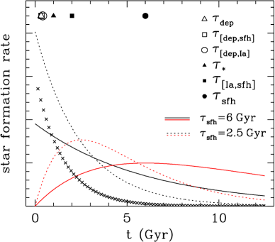
Figure 1.— Star formation histories and timescales. The solid black curve shows the SFH of our fiducial model, an exponential with $\tau_{\rm sfh}=6\,{\rm Gyr}$. The dotted black curve shows a $\tau_{\rm sfh}=2.5\,{\rm Gyr}$ exponential, used in some of our examples. Red solid and dotted curves show linear-exponential SFH cases with the same two timescales. SFR units are arbitrary, with all histories normalized to the same integral over $12.5\,{\rm Gyr}$. Crosses show the exponential SNIa DTD with $\tau_{\rm Ia}=1.5\,{\rm Gyr}$ and minimum delay time $t_{D}=0.15\,{\rm Gyr}$ assumed in most of our calculations. Points near the top axis show quantities for the fiducial model: the depletion, SFE, and SFH timescales ($\tau_{\rm dep}$, $\tau_{*}$, $\tau_{\rm sfh}$) and the three harmonic difference timescales $\bar{\tau}_{[{\rm dep,sfh}]}$, $\bar{\tau}_{[{\rm dep,Ia}]}$, $\bar{\tau}_{[{\rm Ia,sfh}]}$.

To set the scene for thinking about evolutionary behavior, Figure 1 compares star formation histories for several of the cases that we consider in our examples of §3.6, and it shows the timescales that govern chemical evolution in our fiducial model. The fiducial model adopts a $6\,{\rm Gyr}$ exponential SFH (solid black curve), SFE timescale $\tau_{*}=1\,{\rm Gyr}$, and outflow efficiency $\eta=2.5$. The solid red curve shows a linear-exponential SFH with the same $\tau_{\rm sfh}$, which rises to a broad plateau over the range $t\approx 4-11\,{\rm Gyr}$. Dotted curves show exponential and linear-exponential curves with a shorter $e$-folding timescale $\tau_{\rm sfh}=2.5\,{\rm Gyr}$. Production of CCSN elements directly tracks the SFH, while production of iron from SNIa is given by the convolution of the SFH with our fiducial DTD, an exponential with $\tau_{\rm Ia}=1.5\,{\rm Gyr}$, shown by crosses. We will see below that the evolution of CCSN abundances is governed by the harmonic difference timescale $\bar{\tau}_{[{\rm dep,sfh}]}$, while the evolution of SNIa iron depends additionally on $\bar{\tau}_{[{\rm dep,Ia}]}$ and $\bar{\tau}_{[{\rm Ia,sfh}]}$. Because of the high $\eta$ adopted in the fiducial model, the depletion time $\tau_{\rm dep}=0.323\,{\rm Gyr}$ is much shorter than $\tau_{\rm sfh}$ or $\tau_{\rm Ia}$. The first two of these timescales are therefore very close to $\tau_{\rm dep}$ itself. The longest timescale in the fiducial model is $\bar{\tau}_{[{\rm Ia,sfh}]}=2\,{\rm Gyr}$, so the iron abundance approaches equilibrium on a timescale that is much longer than that of oxygen but still short compared to the SFH timescale and the age of the Galaxy.

While a constant SFR is just the limiting case of an exponential SFH with $\tau_{\rm sfh}\rightarrow\infty$, it is useful to begin with this analytically and physically simpler case.

3.1. Constant SFR

For a constant SFR, and constant $\tau_{*}$ and $\eta$, it is straightforward to solve for the full evolution of the oxygen abundance. It is helpful to first rewrite equation (7) in the form

$$\dot{Z}_{\rm O}+{Z_{\rm O}\over\tau_{\rm dep}}={m_{\rm O}^{\rm cc}\over\tau_{*}}~{},$$ (31)

using the substitutions $\dot{M}_{*}=M_{g}/\tau_{*}$ and $Z_{\rm O}=M_{\rm O}/M_{g}$. We have used the fact that constant SFR and $\tau_{*}$ imply that $\dot{M}_{g}=0$ and thus $\dot{Z}_{\rm O}=\dot{M}_{\rm O}/M_{g}$. The general solution to a differential equation of the form

$$\dot{y}+p(t)y=f(t)$$ (32)

is

$$y(t)={1\over\mu(t)}\left[\int_{0}^{t}\mu(t^{\prime})f(t^{\prime})dt^{\prime}+C\right],\quad\mu(t)=e^{\int p(t)dt}~{},$$ (33)

where in this case we have simply $p(t)=\tau_{\rm dep}^{-1}$, $\mu(t)=e^{t/\tau_{\rm dep}}$, and $f(t)=m_{\rm O}^{\rm cc}\tau_{*}^{-1}$. Setting the integration constant $C=0$ corresponds to setting $Z_{\rm O}=0$ at $t=0$. With this initial condition, the solution is

$$Z_{\rm O}(t)={m_{\rm O}^{\rm cc}\over(1+\eta-r)}\left[1-e^{-t/\tau_{\rm dep}}\right],$$ (34)

which approaches the equilibrium abundance $Z_{\rm O,eqc}$ on a gas depletion timescale $\tau_{\rm dep}=\tau_{*}/(1+\eta-r)$. Larson (1972) derives an equivalent equation for the case $\eta=r=0$. (For further discussion of the relation to previous analytic results see §3.5.) Starting from a non-zero abundance adds a term $Z_{O,{\rm init}}e^{-t/\tau_{\rm dep}}$ to equation (34).

For iron, it is useful to consider the evolution of the core collapse and SNIa contributions separately, with the total iron abundance being simply the sum of the two. The core collapse contribution follows the same evolution as the oxygen abundance:

$$Z_{\rm Fe}^{\rm cc}(t)={m_{\rm Fe}^{\rm cc}\over(1+\eta-r)}\left[1-e^{-t/\tau_{\rm dep}}\right].$$ (35)

At times $t<t_{D}$, there is no SNIa contribution, and the abundance ratio is just determined by the CCSN yields, $Z_{\rm O}/Z_{\rm Fe}=m_{\rm O}^{\rm cc}/m_{\rm Fe}^{\rm cc}$.

For the evolution of the SNIa iron contribution, a similar set of substitutions in equation (8) yields

$$\dot{Z}_{\rm Fe}^{\rm Ia}+{Z_{\rm Fe}^{\rm Ia}\over\tau_{\rm dep}}={m_{\rm Fe}^{\rm Ia}\over\tau_{*}}{\langle\dot{M}_{*}\rangle_{\rm Ia}\over\dot{M}_{*}}={m_{\rm Fe}^{\rm Ia}\over\tau_{*}}\left[1-e^{-\Delta t/\tau_{\rm Ia}}\right]~{},$$ (36)

where the second equality uses $\langle\dot{M}_{*}\rangle_{\rm Ia}$ for an exponential SNIa DTD with constant SFR and $\Delta t=t-t_{D}$ (see equation 10). With a slightly tedious but straightforward calculation, one can use the same method to solve this differential equation with the boundary condition $Z_{\rm Fe}^{\rm Ia}=0$ at $\Delta t=0$. The result can be expressed in the form

$$\begin{split}Z_{\rm Fe}^{\rm Ia}(t)=&{m_{\rm Fe}^{\rm Ia}\over 1+\eta-r}\Big{[}1-e^{-\Delta t/\tau_{\rm dep}}-\\ &{\bar{\tau}_{[{\rm dep,Ia}]}\over\tau_{\rm dep}}\left(e^{-\Delta t/\tau_{\rm Ia}}-e^{-\Delta t/\tau_{\rm dep}}\right)\Big{]}~{},\end{split}$$ (37)

with $\bar{\tau}_{[{\rm dep,Ia}]}$ defined by equation (23), subject to the condition $\tau_{\rm dep}\neq\tau_{\rm Ia}$.

It is evident from equation (37) that the equilibrium iron abundance is reached only when $\Delta t\gg\tau_{\rm dep}$ and $\Delta t\gg\tau_{\rm Ia}$, i.e., the timescale to reach equilibrium is controlled by the longer of the gas depletion timescale and the SNIa timescale. In the limiting cases of $\tau_{\rm Ia}\ll\tau_{\rm dep}$ or $\tau_{\rm dep}\ll\tau_{\rm Ia}$, the factor $\bar{\tau}_{[{\rm dep,Ia}]}/\tau_{\rm dep}$ goes to 0 or 1 respectively, and equation (37) yields the pleasingly intuitive results

$$Z_{\rm Fe}^{\rm Ia}(t) = {m_{\rm Fe}^{\rm Ia}\over 1+\eta-r}\left[1-e^{-\Delta t/\tau_{\rm dep}}\right],\quad\tau_{\rm Ia}\ll\tau_{\rm dep},$$ (38)

$$Z_{\rm Fe}^{\rm Ia}(t) = {m_{\rm Fe}^{\rm Ia}\over 1+\eta-r}\left[1-e^{-\Delta t/\tau_{\rm Ia}}\right],\quad\tau_{\rm dep}\ll\tau_{\rm Ia}.$$ (39)

In the former case, SNIa enrichment is effectively instantaneous after $t_{D}$, so the evolution is simply a shifted version of the core collapse evolution (35) with the SNIa yield in place of the CCSN yield. In the latter case, evolution to equilibrium is controlled instead by the SNIa timescale.

For many realistic situations we expect $\tau_{\rm Ia}$ and $\tau_{\rm dep}$ to be of similar order. Equation (37) looks it could diverge for $\tau_{\rm dep}\approx\tau_{\rm Ia}$, but rearranging and Taylor expanding the exponentials shows that when $\Delta t\ll|\bar{\tau}_{[{\rm dep,Ia}]}|$ the solution approaches

$$Z_{\rm Fe}^{\rm Ia}(t)\approx{m_{\rm Fe}^{\rm Ia}\over 1+\eta-r}\left[1-e^{-\Delta t/\tau_{\rm dep}}-{\Delta t\over\tau_{\rm dep}}e^{-\Delta t/\tau_{\rm dep}}\right]~{},$$ (40)

so there is no divergence.

At early times when $\Delta t\ll\tau_{\rm dep}$ and $\Delta t\ll\tau_{\rm Ia}$, Taylor expanding all of the exponentials in equation (37) shows that $Z_{\rm Fe}^{\rm Ia}(t)=0$ to first order in $\Delta t$. Expanding to second order yields

$$Z_{\rm Fe}^{\rm Ia}(t)\approx{m_{\rm Fe}^{\rm Ia}\over 1+\eta-r}\cdot{1\over 2}{\Delta t\over\tau_{\rm Ia}}{\Delta t\over\tau_{\rm dep}},\qquad\Delta t\ll\tau_{\rm Ia},~{}\Delta t\ll\tau_{\rm dep}~{}.$$ (41)

In this sense, SNIa enrichment “turns on slowly” starting at $t=t_{D}$, so the “knee” in an $[{\rm O}/{\rm Fe}]-[{\rm Fe}/{\rm H}]$ diagram is a smooth bend rather than a discontinuous change of slope (see Fig. 2 below).

Since core collapse iron follows the same evolution as core collapse oxygen, the drop in $[{\rm O}/{\rm Fe}]$ relative to the early-time CCSN plateau is determined by the ratio of SNIa iron to core collapse iron:

$$\Delta[{\rm O}/{\rm Fe}]=-\log_{10}\left[1+Z_{\rm Fe}^{\rm Ia}(t)/Z_{\rm Fe}^{\rm cc}(t)\right]~{},$$ (42)

where we have defined

$$\Delta[{\rm O}/{\rm Fe}]\equiv[{\rm O}/{\rm Fe}]-[{\rm O}/{\rm Fe}]_{\rm plateau}$$ (43)

and

$$[{\rm O}/{\rm Fe}]_{\rm plateau}=\log_{10}\left[\frac{m_{\rm O}^{\rm cc}/m_{\rm Fe}^{\rm cc}}{Z_{\rm O,\odot}/Z_{\rm Fe,\odot}}\right]~{}.$$ (44)

The late time result, in equilibrium, is

$$\Delta[{\rm O}/{\rm Fe}]=-\log_{10}\left[1+m_{\rm Fe}^{\rm Ia}/m_{\rm Fe}^{\rm cc}\right],\quad t\gg\tau_{\rm dep}~{}.$$ (45)

The change in $[{\rm O}/{\rm Fe}]$ depends only on the iron yields, not the oxygen yields; for our adopted yields $m_{\rm Fe}^{\rm cc}=0.0012$ and $m_{\rm Fe}^{\rm Ia}=0.0017$ the drop is 0.38 dex for a constant SFR. Relative to the low metallicity plateau, the evolution of $[{\rm X}/{\rm Fe}]$ should be the same for any element X whose production is dominated by CCSNe, provided the IMF stays constant in time and the element’s yield is independent of metallicity. Departures from this behavior could be a useful diagnostic for element production mechanisms or IMF changes. We return to this point in §5.4.

For small $\Delta t$ (specifically $Z_{\rm Fe}^{\rm Ia}/Z_{\rm Fe}^{\rm cc}\ll 1$, $\Delta t\ll\tau_{\rm dep}$, and $\Delta t\ll\tau_{\rm Ia}$), we can use a Taylor expansion of equation (42) together with equations (35) and (41) to approximate the evolution of $[{\rm O}/{\rm Fe}]$ near the knee, obtaining

$$\Delta[{\rm O}/{\rm Fe}]\approx-{m_{\rm Fe}^{\rm Ia}/m_{\rm Fe}^{\rm cc}\over 2\ln 10}{(\Delta t)^{2}\over\tau_{\rm Ia}\tau_{\rm dep}}\times\left(1-e^{-t/\tau_{\rm dep}}\right)^{-1}~{},$$ (46)

with $t\approx t_{D}$. Thus, the initial turndown of the $[{\rm O}/{\rm Fe}]$ track is quadratic in $\Delta t$. The full expression based on combining equations (37) and (35) is not especially illuminating, but in the limiting cases represented by equations (38) and (39) we obtain, respectively,

$$\Delta[{\rm O}/{\rm Fe}]\approx-\log_{\rm 10}\left[1+{m_{\rm Fe}^{\rm Ia}\over m_{\rm Fe}^{\rm cc}}{\left(1-e^{-\Delta t/\tau_{\rm dep}}\right)\over\left(1-e^{-t/\tau_{\rm dep}}\right)}\right]~{}$$ (47)

for $\tau_{\rm Ia}\ll\tau_{\rm dep}$ and

$$\Delta[{\rm O}/{\rm Fe}]\approx-\log_{\rm 10}\left[1+{m_{\rm Fe}^{\rm Ia}\over m_{\rm Fe}^{\rm cc}}{\left(1-e^{-\Delta t/\tau_{\rm Ia}}\right)\over\left(1-e^{-t/\tau_{\rm dep}}\right)}\right]$$ (48)

for $\tau_{\rm dep}\ll\tau_{\rm Ia}$. In the former case, the abundance drop approaches its equilibrium value by the time $\Delta t\approx t$ (i.e., $t\gg t_{D}$), while in the latter case the approach to equilibrium depends mainly on $\Delta t/\tau_{\rm Ia}$.

3.2. Exponentially declining SFR

When considering time-dependent SFR, we assume that the time dependence is driven by a time-dependent gas supply $M_{g}(t)$, with constant $\tau_{*}$. (See §5.5 for a time-dependent $\tau_{*}$ case.) It is most straightforward to solve for the metal mass evolution itself, then divide by $M_{g}(t)$ to get the evolving abundance. In the case of oxygen, substituting $\dot{M}_{*}(t)=M_{g}(t)/\tau_{*}$ and $Z_{\rm O}=M_{\rm O}(t)/M_{g}(t)$ in equation (7) yields

$$\dot{M}_{\rm O}+{M_{\rm O}\over\tau_{\rm dep}}=m_{\rm O}^{\rm cc}{M_{g}(t)\over\tau_{*}}~{}.$$ (49)

The solution proceeds like the above solution for $Z_{\rm O}(t)$ with constant SFR, but now the driving function $f(t)$ in equation (32) is $m_{\rm O}^{\rm cc}M_{g}(t)/\tau_{*}$ instead of simply $m_{\rm O}^{\rm cc}/\tau_{*}$. For an exponential star formation history we have $M_{g}(t)=M_{g0}e^{-t/\tau_{\rm sfh}}$, and a short calculation yields the solution (assuming $\tau_{\rm sfh}\neq\tau_{\rm dep}$)

$$Z_{\rm O}(t)=Z_{\rm O,eq}\left[1-e^{-t/\bar{\tau}_{[{\rm dep,sfh}]}}\right]~{},$$ (50)

with $Z_{\rm O,eq}$ given by equation (28) and

$$\bar{\tau}_{[{\rm dep,sfh}]}\equiv\left(\tau_{\rm dep}^{-1}-\tau_{\rm sfh}^{-1}\right)^{-1}~{}.$$ (51)

This solution has the same form as equation (34) for constant SFR, but the equilibrium abundance is now the higher one from equation (15), and the timescale for approaching equilibrium is $\bar{\tau}_{[{\rm dep,sfh}]}$ rather than $\tau_{\rm dep}$. Provided there is continuing gas accretion, we expect $\tau_{\rm sfh}>\tau_{\rm dep}$, and if $\tau_{\rm sfh}\gg\tau_{\rm dep}$ then $\bar{\tau}_{[{\rm dep,sfh}]}\approx\tau_{\rm dep}$. However, if $\tau_{\rm sfh}\approx\tau_{\rm dep}$, as expected for a very low gas accretion rate, then the equilibrium abundance itself is high because $\tau_{*}/\tau_{\rm sfh}\approx 1+\eta-r$, and the timescale for reaching that abundance is long ($\bar{\tau}_{[{\rm dep,sfh}]}\gg\tau_{\rm dep}$) because the enrichment rate is evolving on the same timescale as the gas supply itself.

If gas is being swept from the system by ram pressure stripping, or by some other process not associated with star formation, then $\tau_{\rm sfh}$ can in principle be shorter than $\tau_{\rm dep}$. In this case $\bar{\tau}_{[{\rm dep,sfh}]}$ is negative, but equation (50) still yields a positive result because both the pre-factor and the factor in $[~{}]$ change sign.

For iron, it is again useful to separate the evolution of the CCSN contribution and the SNIa contribution. The former has the same behavior as oxygen,

$$Z_{\rm Fe}^{\rm cc}(t)=Z^{\rm cc}_{\rm Fe,eq}\left[1-e^{-t/\bar{\tau}_{[{\rm dep,sfh}]}}\right]~{}.$$ (52)

The solution for SNIa is somewhat tedious because there are three exponential timescales involved, $\tau_{\rm dep}$, $\tau_{\rm Ia}$, and $\tau_{\rm sfh}$, and they enter in several different combinations. The end result is

$$\begin{split}Z_{\rm Fe}^{\rm Ia}(t)=&Z^{\rm Ia}_{\rm Fe,eq}\Big{[}1-e^{-\Delta t/\bar{\tau}_{[{\rm dep,sfh}]}}\\ &-{\bar{\tau}_{[{\rm dep,Ia}]}\over\bar{\tau}_{[{\rm dep,sfh}]}}\left(e^{-\Delta t/\bar{\tau}_{[{\rm Ia,sfh}]}}-e^{-\Delta t/\bar{\tau}_{[{\rm dep,sfh}]}}\right)\Big{]}~{}.\end{split}$$ (53)

In the limit that $\tau_{\rm sfh}$ is much larger than $\tau_{\rm Ia}$ and $\tau_{\rm dep}$, the harmonic difference timescales simplify to $\bar{\tau}_{[{\rm dep,sfh}]}\approx\tau_{\rm dep}$ and $\bar{\tau}_{[{\rm Ia,sfh}]}\approx\tau_{\rm Ia}$, making equation (53) equivalent to equation (37). This is as expected, since an infinite exponential timescale is equivalent to a constant SFR. In the alternative limit that $\tau_{\rm Ia}$ and $t_{D}$ are much shorter than $\Delta t$, $\tau_{\rm dep}$, and $\tau_{\rm sfh}$, the ratio $\bar{\tau}_{[{\rm dep,Ia}]}/\bar{\tau}_{[{\rm dep,sfh}]}\rightarrow 0$, and the solution (53) approaches that for $Z_{\rm Fe}^{\rm cc}(t)$ in equation (52), except for the difference in yield. In this limit, SNIa enrichment is effectively instantaneous, so the distinction from CCSN enrichment goes away. Finally, in the limit that $\tau_{\rm dep}$ is much smaller than either $\tau_{\rm Ia}$ or $\tau_{\rm sfh}$, equation (53) approaches

$$Z_{\rm Fe}^{\rm Ia}(t)=Z^{\rm Ia}_{\rm Fe,eq}\left[1-e^{-\Delta t/\bar{\tau}_{[{\rm Ia,sfh}]}}\right]~{},$$ (54)

with the form of equation (52) but the timescale $\bar{\tau}_{[{\rm Ia,sfh}]}$. While it is not obvious by inspection, equation (53) yields a positive iron abundance even when $\bar{\tau}_{[{\rm Ia,sfh}]}$, and thus $Z^{\rm Ia}_{\rm Fe,eq}$, are negative.

3.3. Linear-Exponential SFR

For the early stages of evolution, it is useful to consider cases in which the gas supply is growing from a small initial value rather than starting at a high value and either staying constant or declining with time. For example, the functional form $te^{-t/\tau_{\rm sfh}}$ provides a better match to the predicted star formation histories of galaxies in semi-analytic models and cosmological simulations than $e^{-t/\tau_{\rm sfh}}$ (Lee et al., 2010; Simha et al., 2014), and at times $t\ll\tau_{\rm sfh}$ this form is just linear in time.

For a linear gas supply $M_{g}(t)\propto t$, our previous solution methods for oxygen abundance yield the result

$$Z_{\rm O}(t)={m_{\rm O}^{\rm cc}\over 1+\eta-r}\left[1-{\tau_{\rm dep}\over t}\left(1-e^{-t/\tau_{\rm dep}}\right)\right]~{},$$ (55)

which has the same equilibrium abundance as the constant SFR solution (eq. 34) but a different evolutionary behavior. At times $t\ll\tau_{\rm dep}$, a 2nd-order Taylor expansion shows that the abundance from equation (55) is just half that for a constant SFR model with the same parameters, because for a given $M_{g}(t)=\tau_{*}\dot{M}_{*}$ the stellar mass formed (and hence CCSN enrichment produced) is just half that formed for a constant gas supply. For oxygen, it is also straightforward to solve the evolution equations for $\dot{M}_{*}(t)\propto te^{-t/\tau_{\rm sfh}}$, with the result

$$Z_{\rm O}(t)=Z_{\rm O,eq}\left[1-{\bar{\tau}_{[{\rm dep,sfh}]}\over t}\left(1-e^{-t/\bar{\tau}_{[{\rm dep,sfh}]}}\right)\right]~{},$$ (56)

where $Z_{\rm O,eq}$ is the equilibrium abundance (28) for the exponentially declining SFH. In the limit of $\tau_{\rm sfh}\gg\tau_{\rm dep}$ this approaches the result for pure linear evolution as expected. In general, the oxygen abundance for a linear-exponential SFH is half that of an exponential SFH at early times and approaches the same final equilibrium at a slower pace. For both cases, early time evolution is sensitive to the assumption that CCSN recycling is instantaneous, and it would be altered if the CCSN products take time to rejoin the star-forming phase of the ISM.

For iron, the full solution is cumbersome, but this case is of sufficient physical interest to make the result worth reporting. The CCSN contribution follows the same behavior as oxygen, of course,

$$Z_{\rm Fe}^{\rm cc}(t)=Z^{\rm cc}_{\rm Fe,eq}\left[1-{\bar{\tau}_{[{\rm dep,sfh}]}\over t}\left(1-e^{-t/\bar{\tau}_{[{\rm dep,sfh}]}}\right)\right]~{}.$$ (57)

The solution for SNIa iron involves all three combinations of the depletion, SNIa, and SFH timescales:

$$\begin{split}Z_{\rm Fe}^{\rm Ia}(t)=&Z^{\rm Ia}_{\rm Fe,eq}{\bar{\tau}_{[{\rm Ia,sfh}]}\over t}\times\\ &\bigg{[}{\Delta t\over\bar{\tau}_{[{\rm Ia,sfh}]}}+{\bar{\tau}_{[{\rm dep,Ia}]}\over\bar{\tau}_{[{\rm dep,sfh}]}}e^{-\Delta t/\bar{\tau}_{[{\rm Ia,sfh}]}}+\\ &\left(1+{\bar{\tau}_{[{\rm dep,sfh}]}\over\bar{\tau}_{[{\rm Ia,sfh}]}}-{\bar{\tau}_{[{\rm dep,Ia}]}\over\bar{\tau}_{[{\rm dep,sfh}]}}\right)e^{-\Delta t/\bar{\tau}_{[{\rm dep,sfh}]}}-\\ &\left(1+{\bar{\tau}_{[{\rm dep,sfh}]}\over\bar{\tau}_{[{\rm Ia,sfh}]}}\right)\bigg{]}~{}.\end{split}$$ (58)

The equilibrium abundances in equations (57) and (58) again match those of the exponential cases, given in equations (29) and (30). One can again take the limit of small $t_{D}$ and $\tau_{\rm Ia}$ and find that the SNIa iron evolution follows that of CCSN iron, i.e., equation (58) approaches equation (57) with the substitution $m_{\rm Fe}^{\rm cc}\rightarrow m_{\rm Fe}^{\rm Ia}$. It is also illuminating to consider the limit in which $\tau_{\rm dep}$ is much smaller than both $\tau_{\rm Ia}$ and $\tau_{\rm sfh}$, in which case equation (58) becomes

$$\begin{split}Z_{\rm Fe}^{\rm Ia}(t)\approx Z^{\rm Ia}_{\rm Fe,eq}&\Big{[}{\Delta t\over t}-{\tau_{\rm dep}\over t}\left(1-e^{-t/\tau_{\rm dep}}\right)-\\ &{\bar{\tau}_{[{\rm Ia,sfh}]}\over t}\left(1-e^{-t/\bar{\tau}_{[{\rm Ia,sfh}]}}\right)\Big{]}~{},\end{split}$$ (59)

which is similar in form to equation (57) but with the additional dependence on the timescale $\bar{\tau}_{[{\rm Ia,sfh}]}$.

3.4. Metallicity distribution functions

In many cases we are interested in the distribution of stars as a function of metallicity in addition to the evolution of abundances over time. If the abundance $Z(t)$ is monotonically increasing, then the number of stars born as a function of metallicity will be

$${dN\over dZ}={dN/dt\over dZ/dt}\propto{\dot{M}_{*}\over\dot{Z}}~{}.$$ (60)

For the simplest cases, this distribution can be obtained analytically.

The oxygen abundance evolution for constant SFR can be expressed in the form

$$z_{O}(t)\equiv Z_{\rm O}(t)/Z_{\rm O,eq}=1-e^{-t/\tau_{\rm dep}}~{},$$ (61)

where $Z_{\rm O,eq}=Z_{\rm O,eqc}=m_{\rm O}^{\rm cc}/(1+\eta-r)$. From this we obtain $\dot{z_{O}}\propto(1-z_{O})$, and since $\dot{M}_{*}$ is constant we get

$${dN\over dz_{O}}\propto(1-z_{O})^{-1}~{},$$ (62)

truncated at the value of $z_{O}(t)$ given by equation (61).

For the exponentially declining SFR (eq. 50), the result is similar, but now the equilibrium abundance is that of equation (28) and we must multiply by $\dot{M}_{*}(t)\propto e^{-t/\tau_{\rm sfh}}\propto(1-z_{O})^{\bar{\tau}_{[{\rm dep,sfh}]}/\tau_{\rm sfh}}$, where we have used equation (50) to find $t=-\bar{\tau}_{[{\rm dep,sfh}]}\ln(1-z_{O})$. The result is

$${dN\over dz_{O}}\propto(1-z_{O})^{-1+\bar{\tau}_{[{\rm dep,sfh}]}/\tau_{\rm sfh}}~{}.$$ (63)

In the limit of $\tau_{\rm sfh}\gg\tau_{\rm dep}$ this approaches the constant SFR result as expected, but in general the exponentially declining SFR produces a distribution that is less sharply peaked at the equilibrium abundance, in part because it takes longer to reach equilibrium, but mostly because a smaller fraction of stars are produced at late times. Noting that $\bar{\tau}_{[{\rm dep,sfh}]}/\tau_{\rm sfh}=(\tau_{\rm sfh}/\tau_{\rm dep}-1)^{-1},$ one can see that $\tau_{\rm sfh}=2\tau_{\rm dep}$ is a critical case for which $dN/dz_{O}$ is constant up to the cutoff at $z_{O}(t)$. Note that metallicity distribution functions (MDFs) are frequently plotted as histograms in logarithmic bins of metallicity (e.g., bins of $[{\rm Fe}/{\rm H}]$), which show $dN/d\ln Z\propto Z\,dN/dZ$. Analytic expressions for the population mean metallicity corresponding to equations (62) and (63) appear in §5.3 below.

Qian & Wasserburg (2012) present analytic forms for the MDF with instantaneous recycling and enrichment using essentially the same methods that we have used here for oxygen, though with quite different notation. Unfortunately, the other cases we have considered do not allow an analytic expression for $t$ or $dz_{O}/dt$ in terms of $z_{O}$, so there is no closed form for the oxygen MDF in the linear or linear-exponential cases, or for the iron MDF once SNIa enrichment becomes important. However, it is easy to tabulate the analytic solution for $Z(t)$ with equal time steps, then sum $\dot{M}_{*}(t)$ in the desired bins of $Z$ to compute the MDF (see Appendix B).

3.5. Relation to Traditional Analytic Models

Conventional analytic models of chemical evolution adopt the instantaneous recycling approximation for all elements, both CCSN and SNIa products, so they should be comparable to our results for oxygen evolution. However, the connection to traditional analytic models has some illuminating subtleties. Binney & Merrifield (1998, §5.3) review the “closed box” (Talbot & Arnett, 1971), “leaky box” (Hartwick, 1976), and “accreting box” (Larson, 1972) models (see also the classic and still illuminating chemical evolution review of Tinsley 1980). The leaky box allows outflow but no inflow, and the closed box is the limiting case with $\eta=0$. For constant $\tau_{*}$, which is assumed in our models, the star formation rate from an initial gas mass $M_{i}$ is

$$\dot{M}_{*}(t)={M_{g}(t)\over\tau_{*}}={1\over\tau_{*}}\left[M_{i}-(1+\eta)\int_{0}^{t}dt^{\prime}\,\dot{M}_{*}(t^{\prime})\right]~{},$$ (64)

where we have set the recycling fraction $r=0$. The solution to this equation is

$$\dot{M}_{*}(t)={M_{i}\over\tau_{*}}e^{-t/\tau_{\rm dep}}~{},$$ (65)

an exponentially declining star formation history with $\tau_{\rm sfh}=\tau_{\rm dep}$. This is precisely the case that is not allowed in our analytic expressions because $\bar{\tau}_{[{\rm dep,sfh}]}$ diverges, but we can consider the limit in which $\tau_{\rm sfh}$ approaches $\tau_{\rm dep}$ from above, so that $t/\bar{\tau}_{[{\rm dep,sfh}]}\rightarrow 0$. Taylor-expanding equation (50) with expression (28) for $Z_{\rm O,eq}$ yields

$$\begin{split}Z_{\rm O}(t)&=Z_{\rm O,eq}\left[1-e^{-t/\bar{\tau}_{[{\rm dep,sfh}]}}\right]\\ &\approx m_{\rm O}^{\rm cc}{\bar{\tau}_{[{\rm dep,sfh}]}\over\tau_{*}}\times{t\over\bar{\tau}_{[{\rm dep,sfh}]}}=m_{\rm O}^{\rm cc}{t\over\tau_{*}}~{}.\end{split}$$ (66)

Defining $f_{g}(t)=M_{g}(t)/M_{i}=e^{-t/\tau_{\rm dep}}$ and substituting $\tau_{*}=(1+\eta)\tau_{\rm dep}$ leads to the conventional expression for the leaky box model,

$$Z_{\rm O}(t)=-{m_{\rm O}^{\rm cc}\over 1+\eta}\ln f_{g}(t)~{},$$ (67)

where the quantity $m_{\rm O}^{\rm cc}/(1+\eta)$ is usually referred to as the “effective yield.”

Next consider our expression (63) for the oxygen MDF. In the leaky box limit $\tau_{\rm sfh}\rightarrow\tau_{\rm dep}$ and $\bar{\tau}_{[{\rm dep,sfh}]}\rightarrow\infty$,

$$z_{O}={Z_{\rm O}\over Z_{\rm O,eq}}={Z_{\rm O}\over m_{\rm O}^{\rm cc}}{\tau_{*}\over\bar{\tau}_{[{\rm dep,sfh}]}}={Z_{\rm O}(1+\eta)\over m_{\rm O}^{\rm cc}}{\tau_{\rm dep}\over\bar{\tau}_{[{\rm dep,sfh}]}}\ll 1~{},$$ (68)

i.e., $Z_{\rm O}$ is always $\ll Z_{\rm O,eq}$ because the latter diverges. Defining $q=\bar{\tau}_{[{\rm dep,sfh}]}/\tau_{\rm sfh}\approx\bar{\tau}_{[{\rm dep,sfh}]}/\tau_{\rm dep}$ allows us to approximate

$${dN\over dZ_{\rm O}}\propto(1-y)^{-1+\bar{\tau}_{[{\rm dep,sfh}]}/\tau_{\rm sfh}}\approx\left(1-{Z_{\rm O}(1+\eta)/m_{\rm O}^{\rm cc}\over q}\right)^{q}~{}.$$ (69)

Applying the $n\rightarrow\infty$ limit $(1-x/n)^{n}\approx e^{-x}$ yields the final result

$${dN\over dZ_{\rm O}}\propto\exp\left[-{Z_{\rm O}\over m_{\rm O}^{\rm cc}/(1+\eta)}\right]~{},$$ (70)

an exponentially declining MDF with effective yield $m_{\rm O}^{\rm cc}/(1+\eta)$. This again matches the conventional leaky box result. Although expression (50) for $Z_{\rm O}(t)$ applies for the constant $\tau_{*}$ assumed in our modeling, the expressions (67) and (70) apply to a no-inflow box regardless of the star formation history.

For constant $\tau_{*}$, the “accreting box” model with constant gas mass is identical to our constant SFR model with $\eta=r=0$. At time $t$, the total mass is

$$M_{t}(t)=M_{g}+\int_{0}^{\infty}\dot{M}_{*}(t^{\prime})dt^{\prime}=M_{g}(1+t/\tau_{*})~{}.$$ (71)

Equation (5.5.8) of Binney & Merrifield (1998) is, in our notation,

$$Z_{\rm O}=m_{\rm O}^{\rm cc}\left[1-\exp\left(1-{M_{t}\over M_{g}}\right)\right]~{},$$ (72)

which in combination with equation (71) yields $Z_{\rm O}=m_{\rm O}^{\rm cc}(1-e^{-t/\tau_{*}})$, equivalent to our equation (34) for $\eta=r=0$. The closed box and leaky box scenarios are fuel-starved, and they have falling $dN/dZ$ because they form a small fraction of their stars at late times. The accreting box scenario, by contrast, has a rising $dN/dZ$.

While the notation and focus is different, our oxygen results overlap those of classic analytic models based on the instantaneous recycling approximation, such as the work of Lynden-Bell (1975), Pagel & Patchett (1975), Tinsley (1975), and Tinsley & Larson (1978). Many of these papers focus on the metallicity distribution function and the relation between metallicity and gas fraction, while here we focus on time evolution. More similar in formulation is the work of, e.g., Recchi et al. (2008) and Spitoni (2015), who build on analytic models from Matteucci (2001) to examine a variety of enriched infall scenarios, of which only the simplest case is considered here (see §5.2). In these papers, our assumption of constant SFE timescale $\tau_{*}$ is described as a “linear Schmidt law.” Qian & Wasserburg’s (2012) formulation is also similar to ours and yields similar results for oxygen evolution and the corresponding MDF. Our analytic results for iron evolution with an exponential SNIa DTD are, to our knowledge, new, and they underlie most of the key findings of this paper.

3.6. Illustrations

We now illustrate the behavior of our analytic solutions for a variety of parameter choices. Unless otherwise specified, all calculations in this section adopt yield parameters $m_{\rm O}^{\rm cc}=0.015$, $m_{\rm Fe}^{\rm cc}=0.0012$, $m_{\rm Fe}^{\rm Ia}=0.0017$ and recycling fraction $r=0.4$. These population-averaged yields correspond to those computed by AWSJ for a Kroupa (2001) IMF with mass limits $0.1-100M_{\odot}$ and the SN yields of Chieffi & Limongi (2004) and Iwamoto et al. (1999, the W70 model). We discuss the choice of recycling fraction further in §3.7. As a fiducial case for comparison to others we adopt outflow parameter $\eta=2.5$, SFE timescale $\tau_{*}=1\,{\rm Gyr}$, an exponentially declining SFH with $\tau_{\rm sfh}=6\,{\rm Gyr}$, and SNIa parameters $\tau_{\rm Ia}=1.5\,{\rm Gyr}$ and $t_{D}=0.15\,{\rm Gyr}$. These are the same parameters as in the fiducial model of AWSJ. We use the solar photospheric abundance scale of Lodders (2003), corresponding to solar mass fractions of 0.0056 for oxygen and 0.0012 for iron (8.69 and 7.47 on the conventional $12+\log(X/H)$ number density scale). Note that there are significant uncertainties in supernova yields, photospheric solar abundances, and corrections for diffusion to connect photospheric abundances to proto-solar abundances, which can easily affect predicted values of $[{\rm O}/{\rm Fe}]$ and $[{\rm Fe}/{\rm H}]$ at the 0.1-dex level or larger, though potential corrections typically take the form of constant offsets in these logarithmic quantities.

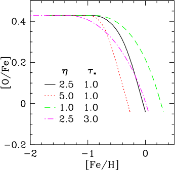
Figure 2.— Tracks in the $[{\rm O}/{\rm Fe}]-[{\rm Fe}/{\rm H}]$ plane for our fiducial model, which has $\eta=2.5$, $\tau_{*}=1\,{\rm Gyr}$, $\tau_{\rm sfh}=6\,{\rm Gyr}$, $\tau_{\rm Ia}=1.5\,{\rm Gyr}$, and $t_{D}=0.15\,{\rm Gyr}$ (black curve), and for alternative models that have a higher outflow rate ($\eta=5$, red dotted curve, lower equilibrium abundance), a lower outflow rate ($\eta=1.0$, green dashed curve, higher equilibrium abundance), or a longer SFE timescale ($\tau_{*}=3\,{\rm Gyr}$, magenta dot-dashed curve, with a “knee” at lower $[{\rm Fe}/{\rm H}]$).

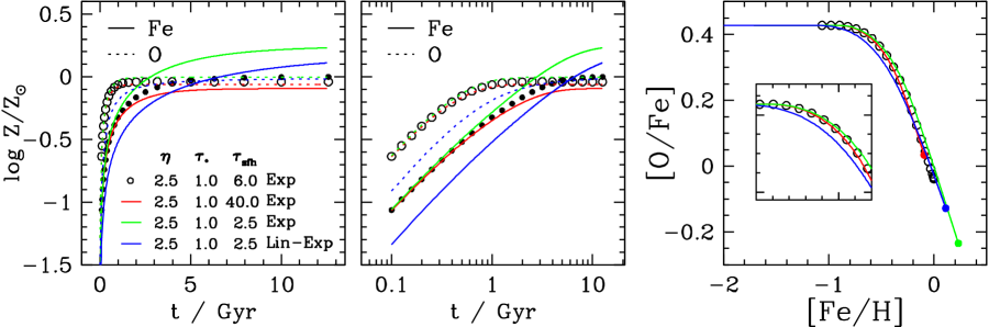
Figure 3.— Abundance evolution (left two panels, with linear time axis on the left and logarithmic time axis in the middle) and $[{\rm O}/{\rm Fe}]-[{\rm Fe}/{\rm H}]$ tracks (right panel) for the fiducial model and three variants. In the left and middle panels, dotted and solid curves show oxygen and iron abundances, respectively; the fiducial model is represented by open and filled circles for visual clarity. In the right panel, the fiducial model is represented by open circles, and filled circles on the other three tracks mark the abundances reached at $t=12.5\,{\rm Gyr}$. The alternative models have $\tau_{\rm sfh}=40\,{\rm Gyr}$, approximating a constant SFR (red curves), a rapidly declining SFH with $\tau_{\rm sfh}=2.5\,{\rm Gyr}$ (green curves), and a model with $\tau_{\rm sfh}=2.5\,{\rm Gyr}$ but a linear-exponential SFH (blue curves). The inset in the right panel presents a magnified view of the knee in the $[{\rm O}/{\rm Fe}]-[{\rm Fe}/{\rm H}]$ tracks. All models have $\tau_{\rm Ia}=1.5\,{\rm Gyr}$ and $t_{D}=0.15\,{\rm Gyr}$.

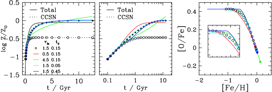
Figure 4.— Similar to Fig. 3, but comparing the fiducial model (circles) to models with different SNIa delay timescales ($\tau_{\rm Ia}=0.5\,{\rm Gyr}$, red curves; $\tau_{\rm Ia}=4.5\,{\rm Gyr},$ green curves) or different SNIa minimum delay times ($t_{D}=0.05\,{\rm Gyr}$, cyan curves; $t_{D}=0.45\,{\rm Gyr}$, blue curves). In the left and middle panels, the open circles and dotted curve show the iron abundance from CCSNe only, which is the same in all six models, while filled circles and solid curves show the total iron abundance including SNIa.

Figure 2 reproduces one of the key results from AWSJ (cf. their figure 3): the end-point of $[{\rm O}/{\rm Fe}]-[{\rm Fe}/{\rm H}]$ tracks is determined principally by the value of $\eta$, while the location of the knee in $[{\rm O}/{\rm Fe}]$ vs. $[{\rm Fe}/{\rm H}]$ is determined principally by the SFE timescale. With $\eta=2.5$ we obtain approximately solar equilibrium abundances for an exponential SFH with $\tau_{\rm sfh}=6\,{\rm Gyr}$, in agreement with AWSJ. Raising (lowering) $\eta$ lowers (raises) the equilibrium value of $[{\rm Fe}/{\rm H}]$ without changing the initial or final values of $[{\rm O}/{\rm Fe}]$. Our adopted CCSN yields produce $[{\rm O}/{\rm Fe}]=+0.43$ on the low-metallicity plateau, and these models end with $[{\rm O}/{\rm Fe}]\approx-0.05$. Tripling $\tau_{*}$ (i.e., lowering the SFE by a factor of three) shifts the location of the knee from $[{\rm Fe}/{\rm H}]\approx-0.8$ to $[{\rm Fe}/{\rm H}]\approx-1.2$ because CCSN have produced less enrichment by the time SNIa enrichment starts to drive down $[{\rm O}/{\rm Fe}]$. Figure 2 shows good qualitative and quantitative agreement with the full numerical results from AWSJ. In AWSJ the equilibrium $[{\rm O}/{\rm Fe}]$ depends slightly (at the 0.05 dex level) on $\eta$, in contrast to the results here. In tests with the numerical code we find that this difference arises from the metallicity dependence of CCSN oxygen yields (ignored in our calculation here), which are reduced at the lower equilibrium metallicity of the $\eta=5$ model.

In Figure 3 we investigate the dependence of chemical enrichment histories on the star formation history. The left and middle panels compare the oxygen and iron evolution for our fiducial model parameters to several alternative models, with time plotted linearly on the left and logarithmically in the middle. The logarithmic time axis provides a better view of early-time evolution, but it can give a misleading visual impression of slow approach to equilibrium by compressing the late-time evolution. The right panel shows the corresponding $[{\rm O}/{\rm Fe}]-[{\rm Fe}/{\rm H}]$ tracks. (See Fig. 1) for the star formation histories themselves.) Starting with the fiducial model, we see that oxygen rises to its equilibrium abundance quickly, on a timescale $\tau_{\rm dep}=\tau_{*}/(1+\eta-r)=0.323\,{\rm Gyr}$, while the iron evolution is controlled by the longer SNIa timescale ($\tau_{\rm Ia}=1.5\,{\rm Gyr}$). Changing to a nearly constant SFR (red curves, with $\tau_{\rm sfh}=40\,{\rm Gyr}$) does not change the early-time behavior, but it slightly lowers the equilibrium oxygen abundance as expected from equation (28). The reduction in the equilibrium iron abundance is larger than for oxygen because at late times a constant SFR yields $\langle\dot{M}_{*}\rangle_{\rm Ia}/\dot{M}_{*}=1$ while the $\tau_{\rm sfh}=6\,{\rm Gyr}$ model has $\langle\dot{M}_{*}\rangle_{\rm Ia}/\dot{M}_{*}\approx\bar{\tau}_{[{\rm Ia,sfh}]}/\tau_{\rm Ia}=2$. As a result, the long-$\tau_{\rm sfh}$ model has a higher equilibrium $[{\rm O}/{\rm Fe}]$, as evident in the right panel.

Green curves show a model with a much more rapid cutoff in star formation, $\tau_{\rm sfh}=2.5\,{\rm Gyr}$. Oxygen evolution is almost unchanged relative to the fiducial model, except for a slight increase in the equilibrium abundance. However, moving $\tau_{\rm sfh}$ closer to $\tau_{\rm Ia}$ increases the harmonic difference timescale $\bar{\tau}_{[{\rm Ia,sfh}]}$ from $2\,{\rm Gyr}$ (fiducial model) to $3.75\,{\rm Gyr}$. The equilibrium iron abundance is therefore substantially higher (eq. 30), but the approach to this equilibrium is much slower. Physically, the high abundance arises because the SNIa iron ejecta are deposited into a rapidly declining gas supply. At $t=12.5\,{\rm Gyr}$, this model has $[{\rm Fe}/{\rm H}]=0.25$ and $[{\rm O}/{\rm Fe}]=-0.25$. Blue curves show the $te^{-t/\tau_{\rm sfh}}$ model, with the same $2.5\,{\rm Gyr}$ timescale. The oxygen abundance is a factor of two lower at early times when the SFR is linearly growing rather than constant, but it approaches the same equilibrium abundance at late times. The iron abundance similarly starts a factor of two below that of the exponential model, and the approach to equilibrium is now very slow, approximately $\propto(1-\bar{\tau}_{[{\rm Ia,sfh}]}/t)$ at late times (see eq. 59). In contrast to the other models plotted, this model remains significantly below the equilibrium abundance at $t=12.5\,{\rm Gyr}$, though it does asymptotically approach the abundance of the exponential SFH model if extended further in time. Except for the endpoints, the $[{\rm O}/{\rm Fe}]-[{\rm Fe}/{\rm H}]$ tracks of all of these models are similar, though the knee for the linear-exponential model is shifted to lower $[{\rm Fe}/{\rm H}]$ because of the slower early enrichment. The model differences here parallel those found in the numerical calculations of AWSJ (their fig. 3).

Figure 4 focuses on the role of the SNIa timescales $\tau_{\rm Ia}$ and $t_{D}$, with other parameters fixed to those of the fiducial model. In the left and middle panels, open circles show the CCSN iron contribution, which is unaffected by the SNIa parameters. In the fiducial model, the total iron (filled circles) begins to depart significantly from the CCSN iron at $t\approx 1\,{\rm Gyr}$, eventually settling to an equilibrium that is 0.5-dex higher. Decreasing or increasing $\tau_{\rm Ia}$ by a factor of three (red and green curves, respectively) shifts the $[{\rm O}/{\rm Fe}]-[{\rm Fe}/{\rm H}]$ knee towards lower or higher $[{\rm Fe}/{\rm H}]$ as expected. For $\tau_{\rm Ia}=4.5\,{\rm Gyr}$, $\bar{\tau}_{[{\rm Ia,sfh}]}$ becomes large (18 Gyr, vs. 2 Gyr for the fiducial model), producing a slow approach to a high equilibrium iron abundance as in the short-$\tau_{\rm sfh}$ model of Figure 3. For $\tau_{\rm Ia}=0.5\,{\rm Gyr}$ the approach to equilbrium is rapid; even though $\tau_{\rm Ia}\approx\tau_{\rm dep}$ in this case, making $\bar{\tau}_{[{\rm dep,Ia}]}$ long, this does not lead to slow evolution (see eq. 40 and associated discussion). Changing $t_{D}$ by a factor of three with fixed $\tau_{\rm Ia}$ does change the onset of the knee in $[{\rm O}/{\rm Fe}]-[{\rm Fe}/{\rm H}]$, but the curves have nearly converged by the time they have dropped $\sim 0.1$-dex below the plateau, and changes to $\tau_{\rm Ia}$ have a larger overall impact on the tracks. We note, however, that the minimum delay time has a larger impact for a $t^{-1.1}$ DTD because the SNIa rate in the power-law model diverges at early times (see §5.1).

Figure 5 plots metallicity distribution functions for the four models shown in Figure 3. The upper left panel shows the distribution of $[{\rm O}/{\rm H}]$, which for exponential SFH models follows equation (63), while the other panels show distributions of $[{\rm Fe}/{\rm H}]$ with a logarithmic or linear $y$-axis. Here the MDF is the fraction of stars born in bins of 0.05-dex in metallicity, proportional to $dN/d\log Z\propto Z\,dN/dZ$. The MDF of the fiducial model rises linearly at early times and is sharply peaked at the equilibrium abundance, for both oxygen and iron. (For $t\ll\tau_{\rm dep}$, the SFR is nearly constant, making $Z\propto t$ and $Z\,dN/dZ\propto Z$.) The peak for iron is less sharp because the timescale for SNIa enrichment is longer, but $\tau_{\rm Ia}$ is still short compared to $\tau_{\rm sfh}=6\,{\rm Gyr}$. For the $\tau_{\rm sfh}=40\,{\rm Gyr}$ model, the equilibrium abundances are lower and the peaks are even sharper.

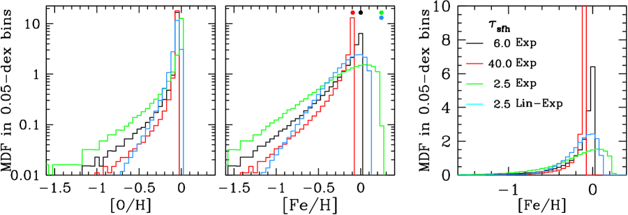
Figure 5.— Metallicity distribution functions (MDFs), computed as the fraction of stars formed in 0.05-dex bins of $[{\rm O}/{\rm H}]$ or $[{\rm Fe}/{\rm H}]$ by $t=12.5\,{\rm Gyr}$ and normalized to unit integral, for the four models shown in Fig. 3. The left and middle panels show the MDFs for oxygen and iron, respectively, while the right panel repeats the iron MDF with a linear vertical axis scale. Note that histograms binned in $[{\rm O}/{\rm H}]$ or $[{\rm Fe}/{\rm H}]$ approximate $Z\,dN/dZ$ rather than $dN/dZ$. In the middle plot, colored dots mark the equilibrium $[{\rm Fe}/{\rm H}]$ of the four models. All models have $\eta=2.5$, $\tau_{*}=1\,{\rm Gyr}$, $\tau_{\rm Ia}=1.5\,{\rm Gyr}$, $t_{D}=0.15\,{\rm Gyr}$.

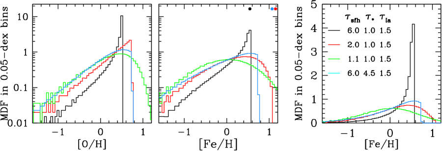
Figure 6.— MDFs as in Fig. 5 for an alternative set of models, all with outflow rate $\eta$ and recycling fraction $r$ set to zero. Black histograms show a model with the same $\tau_{*}=1\,{\rm Gyr}$ and $\tau_{\rm sfh}=6\,{\rm Gyr}$ as our fiducial model, while other curves show models with shorter SFH timescales ($\tau_{\rm sfh}=2\,{\rm Gyr}$, red histograms; $\tau_{\rm sfh}=1.1\,{\rm Gyr}$, green histograms) or a longer SFE timescale ($\tau_{*}=4.5\,{\rm Gyr}$, blue histograms). All models have $\tau_{\rm Ia}=1.5\,{\rm Gyr}$ and $t_{D}=0.15\,{\rm Gyr}$.

Shortening $\tau_{\rm sfh}$ to 2.5 Gyr makes only moderate difference to the oxygen MDF, as this timescale is still much larger than $\tau_{\rm dep}=\tau_{*}/(1+\eta-r)=0.323\,{\rm Gyr}$. However, the peak of the iron MDF changes substantially in this case, in part because of the higher equilibrium abundance, but also because SNIa can still provide significant iron enrichment after the SFR has declined, producing a much softer cutoff of the MDF. The linear-exponential model with the same $\tau_{\rm sfh}$ has the same equilibrium iron abundance as the exponential model, but, as shown previously in Figure 3, it does not reach this abundance by $t=12.5\,{\rm Gyr}$. Its MDF therefore turns over significantly before that of the exponential model. Both the oxygen and iron MDFs rise quadratically at early times because $Z\propto t$, $\dot{M}_{*}\propto t$, and thus $Z\,dN/dZ\propto t^{2}\propto Z^{2}$.

Figure 6 shows MDFs for cases that illustrate a variety of behaviors, where we have set $\eta=r=0$ for simplicity of interpretation. With $\tau_{*}=1\,{\rm Gyr}$ and $\tau_{\rm sfh}=6\,{\rm Gyr}$, the oxygen and iron MDFs are similar to those of our fiducial model except for the $\sim 0.4$-dex increase in equilibrium abundance that results from eliminating outflows. Setting $\tau_{\rm sfh}=2\,{\rm Gyr}=2\tau_{*}$ corresponds to the critical case of constant $dN/dz_{O}$ in equation (63), producing an oxygen MDF that rises linearly until a sharp cutoff at $[{\rm O}/{\rm H}]=0.5$, the enrichment level achieved by $t=12.5\,{\rm Gyr}$. The iron MDF of this model exhibits a smooth turnover instead of a sharp cutoff because of the longer timescale of SNIa, which allows them to produce significant iron even after the star formation rate has fallen substantially. A model with $\tau_{\rm sfh}=3\,{\rm Gyr}=2\tau_{\rm Ia}$ (not shown) produces an iron MDF that is almost linearly rising to a sharp cutoff, similar to the oxygen MDF for $\tau_{\rm sfh}=2\tau_{*}$.

Reducing $\tau_{\rm sfh}$ to $1.1\,{\rm Gyr}=1.1\tau_{*}$ corresponds nearly to a conventional closed box model, which has $\tau_{\rm sfh}=\tau_{*}$ as discussed in §3.5. The form of the oxygen MDF is very close to the closed box form $dN/d\ln Z_{\rm O}\propto Z_{\rm O}\exp(-Z_{\rm O}/m_{\rm O}^{\rm cc})$, where the turnover scale corresponds to $[{\rm O}/{\rm H}]=0.43$ for our adopted values of $m_{\rm O}^{\rm cc}$ and the solar oxygen abundance. In contrast to the other cases we have examined, the iron MDF in this model is nearly symmetric in $[{\rm Fe}/{\rm H}]$, and extremely broad. The substantial change of behavior relative to the previous model arises because $\tau_{\rm sfh}$ has crossed the critical threshold $\tau_{\rm sfh}=\tau_{\rm Ia}$. For this model (and any model with $\tau_{\rm sfh}<\tau_{\rm Ia}$) the equilibrium abundance (eq. 30) is negative, and it no longer represents a late time asymptotic value. Instead, the iron abundance grows exponentially at late times on the timescale $|\bar{\tau}_{[{\rm Ia,sfh}]}|$ because the exponentially declining SNIa enrichment is deposited into a gas supply that is declining exponentially on a still shorter timescale.

The final model in Figure 6 has $\tau_{\rm sfh}=6\,{\rm Gyr}$ but a low star formation efficiency, with $\tau_{*}=4.5\,{\rm Gyr}$. With $\tau_{\rm sfh}/\tau_{*}=1.33$, the oxygen MDF of this model is close to that of the closed box model except that it cuts off sharply at $[{\rm O}/{\rm H}]=0.5$, the abundance reached at $t=12.5\,{\rm Gyr}$. Because the depletion timescale is now much longer than $\tau_{\rm Ia}$, the iron MDF is similar to the oxygen MDF, as SNIa are approximately “instantaneous” compared to the chemical evolution timescale.

The cases in Figures 5 and 6 illustrate several general points about the MDFs of one-zone models. When the depletion time is short and the SFH timescale is long, the MDF is usually sharply peaked near the equilibrium abundance, with a strong negative skewness, as in our fiducial model. Many plausible chemical evolution models fall in this regime of parameter space. A rapidly declining star formation history (short $\tau_{\rm sfh}$) can produce a gentler cutoff and less asymmetry of the MDF. The transition between regimes arises at $\tau_{\rm sfh}\approx 2\tau_{\rm dep}$ for oxygen and $\tau_{\rm sfh}\approx 2\tau_{\rm Ia}$ for iron. A linear-exponential SFH model approaches equilibrium more slowly than an exponential SFH model, so its abundances can remain significantly below equilibrium even at $t\approx 12.5\,{\rm Gyr}$. Inefficient star formation, with long $\tau_{\rm dep}$, can change the shape of MDFs by approaching the regime of $\tau_{\rm sfh}\approx\tau_{\rm dep}$ and by truncating evolution before equilibrium is reached.

In disk galaxies like the Milky Way, radial migration of stars and flows of enriched gas may also play critical roles in shaping MDFs (e.g., Schönrich & Binney 2009; Bilitewski & Schönrich 2012; Pezzulli & Fraternali 2016). A solid understanding of the MDFs of one-zone models is essential background for interpreting constraints on these more complex processes.

3.7. Numerical Tests

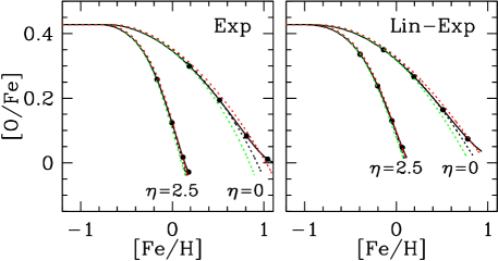
Figure 7.— Tracks in $[{\rm O}/{\rm Fe}]-[{\rm Fe}/{\rm H}]$ for a numerical calculation with continuous AGB recycling (solid curves) and the analytic results with recycling parameters of $r=0.3$, 0.4, and 0.5 (green, black, and red dotted curves), assuming an exponential (left panel) or linear-exponential (right panel) star formation history. In each panel the left set of curves has the parameters of the fiducial model and the right set of curves has the same parameters but no outflow. Points on the solid curves mark $t=1$, 2, 4, and 8 Gyr; curves end at $t=12.5\,{\rm Gyr}$.

To check our analytic solutions and test the impact of our limiting assumptions, we have written a code that numerically integrates the equations for the evolution of oxygen and iron mass for an arbitrary star formation history and mass outflow history. Using this code, we have numerically confirmed our analytic solutions for the time-evolution of the oxygen and iron abundances with a constant, exponential, or linear-exponential SFH. We have also confirmed analytic results that appear later in the paper for evolution with sudden parameter changes (§4.2), with a time-dependent $\tau_{*}$ (§5.5), or with a star formation history that is the sum of exponentials or linear-exponentials (§5.6). With this numerical code we can also relax two of the assumptions needed to allow our analytic solutions: instantaneous return of metals incorporated into stars, and an exponential SNIa DTD.

Figure 7 compares $[{\rm O}/{\rm Fe}]-[{\rm Fe}/{\rm H}]$ tracks from our analytic calculations assuming instantaneous recycling of birth metals to numerical results that incorporate continuous recycling. Specifically, we adopt our usual Kroupa IMF and assume that a star of mass $M$ returns a mass $M-M_{\rm rem}$ of gas to the ISM at its birth metallicity after a time $t=10\,{\rm Gyr}(M/M_{\odot})^{-3.5}$, where the remnant mass is $1.44M_{\odot}$ for stars with $M>8M_{\odot}$ and $0.394M_{\odot}+0.109M$ for $M<8M_{\odot}$ based on Kalirai et al. (2008). While this simple lifetime formula becomes inaccurate at high masses, recycling is fast there in any case, so for our purposes we care mainly about the behavior in the range $M\sim 0.8-2M_{\odot}$. Stars above $8M_{\odot}$ also return newly synthesized oxygen and iron with our standard net yields, as in our analytic calculations.

In each panel of Figure 7 (exponential SFH on the left and linear-exponential on the right, with $\tau_{\rm sfh}=6\,{\rm Gyr}$), the left set of curves shows results for our fiducial outflow rate $\eta=2.5$, which yields near-solar equilibrium abundances. The parameter combination that appears in our analytic solutions is $1+\eta-r$, so with $\eta=2.5$ setting $r=0.3$, 0.4, or 0.5 makes little difference (three dotted curves). Since recycling is a small effect in any case, it is unsurprising that agreement with the continuous recycling result (solid curve) is nearly perfect. The right set of curves sets $\eta=0$ to maximize the impact of recycling. The instantaneous curve with $r=0.4$ (equal to the Kroupa IMF recycling fraction after $2\,{\rm Gyr}$) agrees well with the continuous recycling calculation up to $t=4\,{\rm Gyr}$, but at later times the full calculation yields higher $[{\rm Fe}/{\rm H}]$ and slightly higher $[{\rm O}/{\rm Fe}]$ because of the greater return of metals from stars formed at earlier times. We conclude that our approximation of instantaneous return of birth metals is generally accurate for models that produce near-solar abundances but can fail at the $0.1-0.2$ dex level for models with low outflow efficiency and declining star formation histories.

We investigate the effects of a power-law SNIa DTD in §5.1 below, where we show that this form can be well approximated by a sum of two exponentials, which remains soluble by our techniques.

4. Sudden Events

4.1. Bursts of Star Formation

For a constant SFR, reaching an equilibrium abundance ratio $[{\rm O}/{\rm Fe}]$ requires $\langle\dot{M}_{*}\rangle_{\rm Ia}=\dot{M}_{*}$ so that oxygen and iron are being added to the system at an equal rate. For declining SFR, equilibrium requires $\langle\dot{M}_{*}(t)\rangle_{\rm Ia}/\dot{M}_{*}(t)$ to reach a constant ratio. A burst of star formation — i.e., an increase of $\dot{M}_{*}$ well above its recent trend — will boost $\dot{M}_{*}$ relative to $\langle\dot{M}_{*}\rangle_{\rm Ia}$ and therefore increase CCSN enrichment relative to SNIa enrichment, driving the system to higher $[{\rm O}/{\rm Fe}]$. The “system” here could be an entire dwarf galaxy if the ISM is well mixed throughout. However, it could also be a single molecular cloud, or the kpc-scale star-forming region around a spiral arm. The defining element of the system is the scale over which newly produced metals are retained and mixed into the gas supply. Gilmore & Wyse (1991) highlighted the potential influence of bursty star formation histories on the $[\alpha/{\rm Fe}]$ ratios of dwarf galaxies, though they emphasized the effect of depressed $[\alpha/{\rm Fe}]$ during quiescent phases (see the black curve in Fig. 9 below) rather than enhanced $[\alpha/{\rm Fe}]$ in the bursts themselves.

In this section we consider the impact of an instantaneous burst that converts a fraction $f_{*}$ of the system’s remaining gas into stars. (There are some subtleties to the meaning of “instantaneous,” as discussed below.) This burst of star formation could be induced by a rapid influx of gas, in which case the abundances of the pre-existing gas would be diluted before the burst takes place. For a simple, well defined model, starting from gas mass $M_{g}$ and abundances $Z_{\rm O}$ and $Z_{\rm Fe}$, we (1) convert a fraction $f_{*}$ of the initial gas supply into stars, (2) eject an amount of gas ${\eta^{\prime}}f_{*}M_{g}$ in an outflow at the pre-burst metallicity, and (3) retain a fraction $f_{\rm met}$ of the CCSN ejecta, including their newly produced metals, their original metals, and their original hydrogen and helium. We use primes to distinguish post-burst from pre-burst quantities; thus ${\eta^{\prime}}$ may differ from the outflow parameter $\eta$ that characterized the preceding evolution.

We require $(1+{\eta^{\prime}})f_{*}\leq 1$ so that we do not use up more than 100% of the original gas supply. Of the gas that does not participate in star formation, the fraction ejected is ${\eta^{\prime}}f_{*}M_{g}/[(1-f_{*})M_{g}]={\eta^{\prime}}f_{*}/(1-f_{*})$. If the SN ejecta are well mixed into the ISM before the outflow occurs, then we expect $f_{\rm met}=1-{\eta^{\prime}}f_{*}/(1-f_{*})$. However, in two extreme limits, all CCSN ejecta could escape without entraining much gas, yielding $f_{\rm met}=0$ regardless of ${\eta^{\prime}}$, or the metals could be captured in dense gas around the supernovae while stellar winds or radiation pressure eject the lower density gas of the system, yielding $f_{\rm met}=1$. Note that even for $f_{\rm met}=1$, the pre-burst metals swept up in the outflow are still ejected.

For notational convenience, we define

$$F_{\rm unp}=1-(1+{\eta^{\prime}})f_{*}~{},$$ (73)

the fraction of the pre-existing gas supply that is “unprocessed,” neither formed into stars nor ejected in the associated outflow. The relation between post-burst and pre-burst gas mass, oxygen mass, and iron mass is:

$${M_{g}^{\prime}} = F_{\rm unp}M_{g}+r_{\rm cc}M_{g}f_{*}f_{\rm met}$$ (74)

$${M_{\rm O}^{\prime}} = F_{\rm unp}M_{\rm O}+r_{\rm cc}M_{\rm O}f_{*}f_{\rm met}+m_{\rm O}^{\rm cc}M_{g}f_{*}f_{\rm met}$$ (75)

$${M_{\rm Fe}^{\prime}} = F_{\rm unp}M_{\rm Fe}+r_{\rm cc}M_{\rm Fe}f_{*}f_{\rm met}+m_{\rm Fe}^{\rm cc}M_{g}f_{*}f_{\rm met}.$$ (76)

In each equation, the first term represents the initial gas that remains after star formation and outflow, and the second term represents the return of gas from CCSN ejecta. The quantity $r_{\rm cc}$ is analogous to our previously used recycling parameter $r$ but includes only the contribution from massive stars that produce CCSNe. For a Kroupa IMF and all stars with $M\geq 8M_{\odot}$ exploding as CCSNe, $r_{\rm cc}=0.20$. The final terms in equations (75) and (76) represent the oxygen and iron newly synthesized by CCSNe. The factor $f_{\rm met}$ appears in the second terms of these equations because we assume that all CCSN ejecta are retained with efficiency $f_{\rm met}$, not just the newly synthesized metals within those ejecta.

In the limit that $f_{\rm met}=0$ the abundances are unchanged, because the outflow carries gas at the pre-burst metallicity. In the opposite limit that $F_{\rm unp}\rightarrow 0$, we obtain

$${Z_{\rm O}^{\prime}}={{M_{\rm O}^{\prime}}\over{M_{g}^{\prime}}}\approx{Z_{\rm O}}{r_{\rm cc}+m_{\rm O}^{\rm cc}Z_{\rm O}^{-1}\over r_{\rm cc}}=Z_{\rm O}+{m_{\rm O}^{\rm cc}\over r_{\rm cc}}~{},$$ (77)

with an analogous result for iron. Here we have used the substitution $M_{g}=Z_{\rm O}^{-1}M_{\rm O}=Z_{\rm Fe}^{-1}M_{\rm Fe}$. Note that $m_{\rm O}^{\rm cc}/r_{\rm cc}$ is the mass fraction of newly synthesized oxygen in CCSN ejecta.

The most interesting impact is on the abundance ratio of the ISM following the burst:

$${{Z_{\rm O}^{\prime}}\over{Z_{\rm Fe}^{\prime}}}={Z_{\rm O}\over Z_{\rm Fe}}{\left[F_{\rm unp}+r_{\rm cc}f_{*}f_{\rm met}+m_{\rm O}^{\rm cc}Z_{\rm O}^{-1}f_{*}f_{\rm met}\right]\over\left[F_{\rm unp}+r_{\rm cc}f_{*}f_{\rm met}+m_{\rm Fe}^{\rm cc}Z_{\rm Fe}^{-1}f_{*}f_{\rm met}\right]}~{}.$$ (78)

If the pre-existing metals (first two terms) dominate over the newly produced metals, then the abundance ratio is essentially unchanged. However, if the final terms dominate then ${Z_{\rm O}^{\prime}}/{Z_{\rm Fe}^{\prime}}\rightarrow m_{\rm O}^{\rm cc}/m_{\rm Fe}^{\rm cc}$, returning the abundance ratio to the CCSN plateau.

Figure 8.— Post-burst iron abundance (left) or $[{\rm O}/{\rm Fe}]$ (right) as a function of the fraction $f_{*}$ of the initial gas mass that is converted to stars during the burst. Black curves show the case in which all gas and metals are retained. Red and green curves show cases with an outflow of mass-loading parameter ${\eta^{\prime}}=1$, starting from solar or $0.3\times$solar abundances, respectively. In these cases the maximum $f_{*}$ is $1/(1+{\eta^{\prime}})=0.5$. Solid curves assume that metals and recycled gas from CCSN are ejected with the same efficiency as pre-existing gas, while dotted curves show the case in which all CCSN ejecta are retained. Black curves have been shifted slightly downward, as they would otherwise be obscured by the solid red curve.

Figure 8 shows abundance changes as a function of $f_{*}$. Black curves show an example in which all gas and metals are retained by the system, ${\eta^{\prime}}=0$ and $f_{\rm met}=1$. Starting from solar abundances, converting 50% of the gas into stars boosts $[{\rm Fe}/{\rm H}]$ by 0.15 dex and $[{\rm O}/{\rm Fe}]$ by 0.2 dex. As the conversion efficiency approaches 100%, the abundance ratio approaches the CCSN plateau value $m_{\rm O}^{\rm cc}/m_{\rm Fe}^{\rm cc}$, corresponding to $[{\rm O}/{\rm Fe}]=+0.43$ for our adopted yields and solar abundance scale. Solid red curves show a case with outflow parameter ${\eta^{\prime}}=1$ and $f_{\rm met}=1-{\eta^{\prime}}f_{*}/(1-f_{*})$, i.e., SN metals are ejected with the same efficiency as the overall outflow. In this situation the change of abundances is determined by $f_{*}$ independent of ${\eta^{\prime}}$, so the red curve lies on top of the black curve, but it extends only to the maximum allowed $f_{*}=1/(1+{\eta^{\prime}})=0.5$, where the $[{\rm O}/{\rm Fe}]$ enhancement is 0.25 dex. If all metals are retained ($f_{\rm met}=1$, dotted red curves) then the impact on abundances rises sharply as $f_{*}$ approaches 0.5. Green curves show cases with ${\eta^{\prime}}=1$ starting from abundances of $0.3\times$ solar. Here the burst has a much larger impact, with a $0.35-0.45$ dex boost in $[{\rm O}/{\rm Fe}]$ as $f_{*}$ approaches 0.5, because the newly produced metals are more important compared to the pre-existing metals.

The takeaway message from Figure 8 is that once a population has evolved to roughly solar $[{\rm O}/{\rm Fe}]$, a burst of star formation can readily boost $[{\rm O}/{\rm Fe}]$ by $\sim 0.1-0.3$ dex if it consumes a significant fraction of the available gas and the metals produced by the CCSNe are retained. Gas with low $[{\rm Fe}/{\rm H}]$, perhaps because of dilution by a recent accretion event that triggers the burst, is more susceptible to such a boost. The quantities in Figure 8 represent the post-burst gas phase abundances after CCSN enrichment, so if the star formation is truly instantaneous then all stars in the burst are born with the pre-burst abundances. However, if the star formation extends over a $\sim 40\,{\rm Myr}$ time span comparable to the lives of $8M_{\odot}$ stars, and metals are efficiently mixed, then stars will be born with the whole range of abundances from the initial to the final values. For our calculation here to be reasonably accurate, the timescale of the “burst” need only be short compared to the $\sim 1\,{\rm Gyr}$ timescale on which SNIa enrichment becomes important.

Individual molecular clouds are usually thought to form stars quite inefficiently, with $f_{*}$ of a few percent (Murray, 2011). Furthermore, CCSN ejecta may frequently escape their parent molecular clouds, making $f_{\rm met}$ low. However, the occasional molecular cloud that forms stars with unusually high efficiency and traps its supernova ejecta in dense surroundings could produce some stars with significantly enhanced $[{\rm O}/{\rm Fe}]$. This “cloud burst” phenomenon is a possible explanation for the rare population of $\alpha$-enhanced stars with intermediate ages found in the SDSS-III APOGEE survey (Martig et al., 2015; Chiappini et al., 2015) and in local samples (Haywood et al., 2015). While low star formation efficiency and metal loss may keep these effects small on the scale of individual molecular clouds, they could have a larger impact on the $\sim\hbox{kpc}$ scale of a spiral arm passage, where the CCSN products of many molecular clouds may be trapped and mixed much more rapidly than SNIa enrichment occurs.

Boosting of CCSN abundances by starbursts could play a significant role in the chemical evolution of dwarf galaxies, which frequently show evidence of bursty star formation histories (Weisz et al., 2014). However, the time resolution of inferred star formation histories is usually too coarse to determine whether the starbursts are short compared to $\tau_{\rm Ia}$. The impact on the galaxy depends critically on what happens to the eventual SNIa metals associated with a burst. If these are retained by the galaxy’s star-forming gas, or return to it after fountaining into the halo, then the CCSN metals produced in a burst may only “catch up” with the SNIa metals from a previous burst, and some inter-burst stars could even be born with substantial deficits of $\alpha$ elements (as emphasized by Gilmore & Wyse 1991). Investigation of these issues requires more detailed models of dwarf galaxy evolution, but the distribution of $[\alpha/{\rm Fe}]$ ratios may set interesting constraints on timescales of starbursts and the physics of dwarf galaxy outflows.

The scatter in $[\alpha/{\rm Fe}]$ at fixed $[{\rm Fe}/{\rm H}]$ is hard to constrain precisely because of the difficulty of subtracting observational errors. However, recent studies suggest that this scatter is $<0.05$ dex rms once one separates the high-$\alpha$ (“thick disk”) and low-$\alpha$ (“thin disk”) sequences (Ramírez et al. 2013; Bertran de Lis et al. 2016, submitted; P. Kempski et al., in preparation). Reversing the arguments above, one can use this small observed scatter to set limits on the stochasticity of star formation and metal mixing in the Milky Way and other galaxies.

4.2. Sudden Changes of Model Parameters

The methods employed in §3 can be extended to calculate evolution that incorporates a sudden change in model parameters at a time $t_{c}$. We consider cases in which the star formation history is $\dot{M}_{*}(t)=\dot{M}_{*,1}e^{-t/\tau_{\rm sfh1}}$ for $t\leq t_{c}$, with SFE timescale and outflow parameters $\tau_{*,1}$ and $\eta_{1}$, and $\dot{M}_{*}(t)=\dot{M}_{*,2}e^{-t_{2}/\tau_{\rm sfh2}}$ for $t>t_{c}$, with corresponding parameters $\tau_{*,2}$ and $\eta_{2}$, where $t_{2}\equiv t-t_{c}$ represents time since the transition. We assume that the yields and SNIa timescale $\tau_{\rm Ia}$ stay constant, though it will be obvious from the solutions below how one would incorporate changes in these parameters as well.

It is useful to imagine that stars formed prior to $t_{c}$ produce distinct isotopes from those formed after $t_{c}$. With this artificial assumption, it is obvious that one can separately calculate the evolution of the elements produced by the two separate phases of star formation, then add them together to get the total elemental abundance. Mathematically, this split works because the differential equations for the evolution of oxygen and iron mass are linear.

Before $t_{c}$, the time evolution is simply given by the previous results from §3.2 with the appropriate parameters. At time $t_{c}$ the oxygen mass is

$$M_{\rm O,c}=Z_{\rm O}(t_{c})M_{g}(t_{c})~{},$$ (79)

with $Z_{\rm O}(t_{c})$ evaluated from equation (50) and $M_{g}(t_{c})=\tau_{*,1}\dot{M}_{*,1}e^{-t/\tau_{\rm sfh1}}$. After $t_{c}$, this abundance evolves according to equation (49) but with the source term on the right hand side set to zero, with the solution

$$M_{\rm O,1}(t_{2})=M_{\rm O,c}e^{-t_{2}/\tau_{\rm dep2}}~{}.$$ (80)

If we assume that $M_{g}(t)$ is continuous across $t_{c}$, then the post-$t_{c}$ star formation history requires $M_{g}(t_{2})=M_{g}(t_{c})e^{-t_{2}/\tau_{\rm sfh2}}$. In combination with equation (79), this implies

$$\begin{split}Z_{\rm O,1}(t_{2})&=Z_{\rm O}(t_{c})e^{-t_{2}/\tau_{\rm dep2}}/e^{-t_{2}/\tau_{\rm sfh2}}\\ &=Z_{\rm O}(t_{c})e^{-t_{2}/\bar{\tau}_{[{\rm dep2,sfh2}]}}~{}.\end{split}$$ (81)

Comparing (80) and (81) we see that while the pre-$t_{c}$ oxygen mass evolves on the timescale $\tau_{\rm dep2}$, the corresponding abundance evolves on the longer timescale $\bar{\tau}_{[{\rm dep2,sfh2}]}$.

For stars forming after $t_{c}$, the oxygen evolution equation is identical to the original exponential SFR case but with time variable $t_{2}$ rather than $t$. The solution is therefore equation (50) with the substitution $t\rightarrow t_{2}$ and post-$t_{c}$ values of the parameters:

$$Z_{\rm O,2}(t_{2})=Z_{\rm O,eq2}\left[1-e^{-t_{2}/\bar{\tau}_{[{\rm dep2,sfh2}]}}\right]~{}.$$ (82)

The full solution for $t>t_{c}$ is

$$Z_{\rm O}(t_{2})=Z_{\rm O,1}(t_{2})+Z_{\rm O,2}(t_{2}).$$ (83)

This result makes intuitive sense: the oxygen abundance evolves from its original value at $t_{c}$ to the post-$t_{c}$ equilibrium abundance on the timescale $\bar{\tau}_{[{\rm dep2,sfh2}]}$.

For iron we must consider three separate contributions. The first is iron produced before $t_{c}$, by either CCSNe or SNIa. After $t_{c}$ this component evolves exactly like pre-$t_{c}$ oxygen, so

$$Z_{\rm Fe,1}(t_{2})=Z_{\rm Fe}(t_{c})e^{-t_{2}/\bar{\tau}_{[{\rm dep2,sfh2}]}}~{}.$$ (84)

The second is iron produced by stars that form after $t_{c}$. This follows the usual evolution for an exponential star formation history but with time variable $t_{2}$, thus following equations (52) and (53) with $t\rightarrow t_{2}$, $\Delta t\rightarrow\Delta t_{2}=t_{2}-t_{D}$, and post-$t_{c}$ values for all of the other parameters:

$$\begin{split}Z_{\rm Fe,2}(t_{2})=&Z^{\rm cc}_{\rm Fe,eq2}\left[1-e^{-t/\bar{\tau}_{[{\rm dep2,sfh2}]}}\right]+\\ &Z^{\rm Ia}_{\rm Fe,eq2}\Big{[}1-e^{-\Delta t_{2}/\bar{\tau}_{[{\rm dep2,sfh2}]}}-{\bar{\tau}_{[{\rm dep2,Ia}]}\over\bar{\tau}_{[{\rm dep2,sfh2}]}}\times\\ &\left(e^{-\Delta t_{2}/\bar{\tau}_{[{\rm Ia,sfh2}]}}-e^{-\Delta t_{2}/\bar{\tau}_{[{\rm dep2,sfh2}]}}\right)\Big{]}~{}.\end{split}$$ (85)

The new case is SNIa iron from stars that form before $t_{c}$ but explode after $t_{c}$. For this third contribution the governing equation is

$$\dot{M}_{\rm Fe}+{M_{\rm Fe}\over\tau_{\rm dep2}}=m_{\rm Fe}^{\rm Ia}\langle\dot{M}_{*}(t)\rangle_{\rm Ia}$$ (86)

with

$$\langle\dot{M}_{*}(t)\rangle_{\rm Ia}=\dot{M}_{*,1}\tau_{\rm Ia}^{-1}\int_{0}^{t_{c}}e^{-{t^{\prime}/\tau_{\rm sfh1}}}e^{-(t-t^{\prime}-t_{D})/\tau_{\rm Ia}}dt^{\prime}~{}.$$ (87)

(Compare to equation A6; here we have assumed $t>t_{c}+t_{D}$ in setting the integration limit to $t_{c}$ rather than $t-t_{D}$.) Evaluating the integral gives

$$\langle\dot{M}_{*}(t)\rangle_{\rm Ia}=\dot{M}_{*,1}{\bar{\tau}_{[{\rm Ia,sfh1}]}\over\tau_{\rm Ia}}\left[e^{t_{c}/\bar{\tau}_{[{\rm Ia,sfh1}]}}-1\right]e^{-(t-t_{D})/\tau_{\rm Ia}}~{}.$$ (88)

With the substitution $t_{2}=t-t_{c}$, equation (86) can now be written in the form

$$\dot{M}_{\rm Fe}+{M_{\rm Fe}\over\tau_{\rm dep2}}=Ke^{-t_{2}/\tau_{\rm Ia}}$$ (89)

with

$$K=m_{\rm Fe}^{\rm Ia}\dot{M}_{*,1}{\bar{\tau}_{[{\rm Ia,sfh1}]}\over\tau_{\rm Ia}}\left[e^{t_{c}/\bar{\tau}_{[{\rm Ia,sfh1}]}}-1\right]e^{-(t_{c}-t_{D})/\tau_{\rm Ia}}~{}.$$ (90)

This equation is solved by the usual technique with the boundary condition that $M_{\rm Fe}$ from this contribution starts from zero at $t=t_{c}$. After some manipulation, and dividing by $M_{g}(t_{2})=M_{g}(t_{c})e^{-t_{2}/\tau_{\rm sfh2}}$, one gets

$$\begin{split}Z_{\rm Fe,3}(t_{2})=&Z_{\rm Fe,eq1}^{\rm Ia}\left[1-e^{-t_{c}/\bar{\tau}_{[{\rm Ia,sfh1}]}}\right]e^{t_{D}/\bar{\tau}_{[{\rm Ia,sfh1}]}}\times\\ &{\bar{\tau}_{[{\rm dep2,Ia}]}\over\bar{\tau}_{[{\rm dep1,sfh1}]}}\left[e^{-t_{2}/\bar{\tau}_{[{\rm Ia,sfh2}]}}-e^{-t_{2}/\bar{\tau}_{[{\rm dep2,sfh2}]}}\right]~{},\end{split}$$ (91)

where $Z_{\rm Fe,eq1}^{\rm Ia}$ is the equilibrium abundance of equation (30) evaluated with the pre-$t_{c}$ parameters. For small values of $t_{2}$, Taylor expansion in the final factor gives

$$\begin{split}Z_{\rm Fe,3}(t_{2})\approx&Z_{\rm Fe,eq1}^{\rm Ia}\left[1-e^{-t_{c}/\bar{\tau}_{[{\rm Ia,sfh1}]}}\right]\times\\ &e^{t_{D}/\bar{\tau}_{[{\rm Ia,sfh1}]}}{t_{2}\over\bar{\tau}_{[{\rm dep1,sfh1}]}}~{},\end{split}$$ (92)

which is linear in $t_{2}$ as expected. The full solution for $t>t_{c}$ is

$$Z_{\rm Fe}(t_{2})=Z_{\rm Fe,1}(t_{2})+Z_{\rm Fe,2}(t_{2})+Z_{\rm Fe,3}(t_{2})~{}.$$ (93)

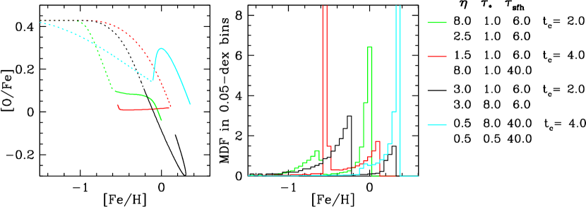
Figure 9.— Tracks in $[{\rm O}/{\rm Fe}]$ vs. $[{\rm Fe}/{\rm H}]$ (left) and iron MDFs (middle) for models with sudden parameter changes, at time $t_{c}$. Parameters before and after $t_{c}$ are listed in the legend at right. In the left panel, dotted and solid lines denote pre-$t_{c}$ and post-$t_{c}$ evolution, respectively. Green curves show a model with a sharp decrease in outflow efficiency $\eta$ and corresponding increase in equilibrium abundance. Red curves show the reverse case, an increase in $\eta$ that drives down the equilibrium abundance. Black curves show a model that transitions from high star formation efficiency ($\tau_{*}=1\,{\rm Gyr}$) to low star formation efficiency ($\tau_{*}=8\,{\rm Gyr}$). Cyan curves show the reverse transition, from $\tau_{*}=8\,{\rm Gyr}$ to $\tau_{*}=0.5\,{\rm Gyr}$.

We can summarize these results as follows. After a sudden change of parameters, the oxygen abundance evolves from its value at $t_{c}$ to the new equilibrium value on the timescale $\bar{\tau}_{[{\rm dep2,sfh2}]}$. The iron abundance has three contributions: exponential decay of $Z_{\rm Fe}(t_{c})$ on the timescale $\bar{\tau}_{[{\rm dep2,sfh2}]}$, growing iron with post-$t_{c}$ parameters that follows the usual behavior for exponential SFR evolution with time variable $t_{2}$, and a contribution from delayed pre-$t_{c}$ SNIa that grows linearly at small $t_{2}$ and then decays exponentially as governed by equation (91). Different choices for parameter changes allow a rich variety of behaviors.

Our assumption that the gas mass is continuous at $t_{c}$ implies that the star formation rate changes discontinuously:

$${\dot{M}_{*}(t_{c}+\epsilon)\over\dot{M}_{*}(t_{c}-\epsilon)}={\tau_{*,1}\over\tau_{*,2}}~{}.$$ (94)

If we instead assume that the gas supply is instantaneously diluted by a factor $D$ at $t_{c}$, so that $M_{g}(t_{c}+\epsilon)/M_{g}(t_{c}-\epsilon)=D$, then the right hand side of this equation is multiplied by $D$. In this case the contributions from pre-$t_{c}$ stars, i.e., the terms $Z_{\rm O,1}$, $Z_{\rm Fe,1}$, and $Z_{\rm Fe,3}$, are divided by $D$, while the contributions $Z_{O,2}$ and $Z_{\rm Fe,2}$ from post-$t_{c}$ stars are unchanged.

Figure 9 presents $[{\rm O}/{\rm Fe}]-[{\rm Fe}/{\rm H}]$ tracks and iron MDFs for several models with sudden parameter changes. Specific parameter values have been chosen partly with regard to keeping the model curves visually distinguishable. Green curves show a model that transitions from high outflow efficiency ($\eta=8$) to our fiducial outflow efficiency ($\eta=2.5$) at $t_{c}=2\,{\rm Gyr}$. The model track progresses rapidly to $[{\rm O}/{\rm Fe}]=0.1$ at $[{\rm Fe}/{\rm H}]\approx-0.6$, but after the change of $\eta$ and the corresponding increase of equilibrium abundance, it turns sharply towards higher $[{\rm Fe}/{\rm H}]$, maintaining approximately constant $[{\rm O}/{\rm Fe}]$. The final downturn comes about $1.5\,{\rm Gyr}$ after the transition, when SNIa enrichment from post-$t_{c}$ star formation drives the model to its final equilibrium abundances of $[{\rm O}/{\rm Fe}]\approx[{\rm Fe}/{\rm H}]\approx 0$, the same as in our fiducial model. The majority of stars are formed close to this final equilibrium. As discussed by AWSJ and Nidever et al. (2014, their Fig. 16), a transition from high-$\eta$ to low-$\eta$ is one of the only ways to create a one-zone model that exhibits substantial growth of $[{\rm Fe}/{\rm H}]$ at near-solar $[{\rm O}/{\rm Fe}]$.

Red curves illustrate the reverse case of a model that approaches equilibrium at low outflow efficiency ($\eta=1.5$) and slightly super-solar $[{\rm Fe}/{\rm H}]$, then tracks backward to low $[{\rm Fe}/{\rm H}]$ at near-constant $[{\rm O}/{\rm Fe}]$ because of an increase in outflow efficiency. The final small uptick, again coming $\approx 1.5\,{\rm Gyr}$ after $t_{c}$, arises because we have also increased $\tau_{\rm sfh}$ from $6\,{\rm Gyr}$ to $40\,{\rm Gyr}$ (i.e., to near-constant SFR), and the latter case leads to higher equilibrium $[{\rm O}/{\rm Fe}]$. If we maintained $\tau_{\rm sfh}=6\,{\rm Gyr}$, the curve would instead downtick to solar $[{\rm O}/{\rm Fe}]$. Progression from high metallicity to low metallicity goes against conventional intuition about chemical evolution, but it is perfectly reasonable if outflow efficiency changes from low to high at late times, which could occur if decreasing gas densities make it easier to drive outflows. However, we have not found a model that produces steadily decreasing $[{\rm Fe}/{\rm H}]$ together with steadily increasing $[{\rm O}/{\rm Fe}]$, resembling the $[\alpha/{\rm Fe}]$ locus for thin disk stars found by, e.g., Adibekyan et al. (2012), Hayden et al. (2015), and Bertran de Lis et al. (2015).

Black curves show a model in which $\eta$ and $\tau_{\rm sfh}$ remain constant but the star formation efficiency changes from high ($\tau_{*}=1\,{\rm Gyr}$) to low ($\tau_{*}=8\,{\rm Gyr}$). After the transition, the model overshoots its original equilibrium, evolving to sub-solar $[{\rm O}/{\rm Fe}]\approx-0.25$ because oxygen enrichment at the low post-$t_{c}$ star formation efficiency is too slow to balance the SNIa iron enrichment coming from pre-$t_{c}$ stars. Since the depletion of this iron is also relatively slow, the model also reaches super-solar $[{\rm Fe}/{\rm H}]\approx+0.25$. The loop upward towards higher $[{\rm O}/{\rm Fe}]$ commences a couple of Gyr after $t_{c}$, but it is a slow change because of the relatively long depletion time, $\tau_{\rm dep}=\tau_{*}/(1+\eta-r)=2.2\,{\rm Gyr}$. In contrast to the other three models in Figure 9, this model has not yet converged to its final (near-solar) equilibrium abundances by the end of the calculation at $t=12.5\,{\rm Gyr}$.

Cyan curves show the opposite transition, from low star formation efficiency ($\tau_{*}=8\,{\rm Gyr}$, $\tau_{\rm dep}=7.3\,{\rm Gyr}$) to high star formation efficiency ($\tau_{*}=0.5\,{\rm Gyr}$, $\tau_{\rm dep}=0.45\,{\rm Gyr}$). The pre-$t_{c}$ evolution has a slow decline in $[{\rm O}/{\rm Fe}]$ characteristic of long-$\tau_{\rm dep}$ models. Although the SFR is nearly constant ($\tau_{\rm sfh}=40\,{\rm Gyr}$) before $t_{c}$ and after $t_{c}$, there is a discontinuous factor of 16 jump in $\dot{M}_{*}$ at the transition (eq. 94). The result is a sudden upward boost of $[{\rm O}/{\rm Fe}]$ like those in the instantaneous burst calculations of §4.1. This trend reverses within a Gyr because of the short post-$t_{c}$ depletion time, and the model quickly evolves to the equilibrium abundances of its post-$t_{c}$ parameters.

The first three of these models produce bimodal MDFs, with one peak corresponding to pre-$t_{c}$ parameters and one to post-$t_{c}$ parameters. Each of these peaks individually has the characteristic form typically seen in Figure 5. For the second (red curve) model, the low metallicity peak corresponds to stars formed after $t_{c}$ and the smaller, high metallicity peak to stars formed before the transition when the equilibrium abundance was high. For the final (cyan curve) model, the two peaks merge into a single distribution because of the low pre-$t_{c}$ star formation efficiency.

5. Extensions

There are a variety of ways that our analytic results can be extended to accommodate interesting cases.

5.1. Two-exponential SNIa Delay Time Distribution

The exponential form of the SNIa DTD is essential to allowing the analytic solutions for iron evolution derived in §3. While this form is reasonably consistent with existing empirical constraints and with the predictions of population synthesis models, it produces fewer supernovae at early times and late times compared to the $t^{-1.1}$ power-law DTD favored by Maoz & Mannucci (2012). Fortunately, it is trivial to generalize the solutions to a DTD that is the sum of two exponential functions with different normalizations and timescales. One simply imagines (purely for convenience) that these two exponentials correspond to two different populations of SNIa that produce distinguishable isotopes of iron: the solution for each population individually is the same as before, and one sums the iron from the two components to obtain the total. Mathematically, the ability to do this follows from the linearity of the governing differential equation.

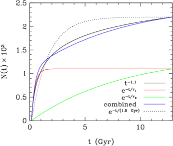
Figure 10.— Cumulative number of SNIa per solar mass of star formation (multiplied by $10^{3}$) as a function of time for our fiducial, $1.5\,{\rm Gyr}$ exponential DTD (dotted black), for a $t^{-1.1}$ power law DTD (solid black), and for the sum of two exponential DTDs with timescales of 0.5 and $5.0\,{\rm Gyr}$ (blue; individual contributions in red and green, respectively). All cases have a minimum delay time $t_{D}=0.15\,{\rm Gyr}$ and are normalized to produce $2.2\times 10^{-3}$ SNIa per solar mass over $12.5\,{\rm Gyr}$.

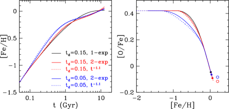
Figure 11.— Evolution of [Fe/H] (left) and tracks in in [O/Fe] vs. [Fe/H] (right) for our fiducial model (black), which has an exponential SNIa DTD, for $t^{-1.1}$ power-law DTDs with minimum delay times $t_{D}=0.15\,{\rm Gyr}$ (red dotted) and $t_{D}=0.05\,{\rm Gyr}$ (blue dotted), and for the matched double-exponential DTDs described in the text (red and blue solid). Except for the DTD, all models have the same parameters as the fiducial model. Filled circles mark the final ($t=12.5\,{\rm Gyr}$) [O/Fe] values for the single- and double-exponential models, and horizontally offset open circles mark the final [O/Fe] values for the power-law DTD models.

Figure 10 compares the cumulative number of SNIa as a function of time from the $t^{-1.1}$ power-law and from a sum of two exponentials with timescales of $0.5\,{\rm Gyr}$ and $5\,{\rm Gyr},$ with a minimum delay time $t_{d}=0.15\,{\rm Gyr}$ in each case. The power-law DTD is normalized to produce $2.2\times 10^{-3}$ SNIa per solar mass of star formation over $12.5\,{\rm Gyr}$, and the two exponentials are individually normalized to produce $1.1\times 10^{-3}$ SNIa per solar mass over the same interval. The two-exponential model approximates the result of the power-law model more closely than our single $1.5\,{\rm Gyr}$ exponential, though it still produces a larger fraction of its SNIa at intermediate times and fewer at early and late times. For a minimum delay of $t_{d}=0.05\,{\rm Gyr}$ (not shown), we obtain comparable agreement by summing two exponentials with timescales of $0.25\,{\rm Gyr}$ and $3.5\,{\rm Gyr}$, again normalized to produce equal numbers of SNIa over $12.5\,{\rm Gyr}$.

Figure 11 compares $[{\rm Fe}/{\rm H}]$ enrichment histories and $[{\rm O}/{\rm Fe}]-[{\rm Fe}/{\rm H}]$ tracks for our fiducial model to numerically calculated results for a $t^{-1.1}$ DTD and to analytic results for the matching two-exponential DTDs described above. For a $0.15\,{\rm Gyr}$ minimum delay time, the $[{\rm Fe}/{\rm H}]$ enrichment is nearly identical between the single-exponential and power-law DTD at early times, with modest differences at $t>2\,{\rm Gyr}$. The most noticeable difference in the $[{\rm O}/{\rm Fe}]-[{\rm Fe}/{\rm H}]$ track is a decrease in the final $[{\rm O}/{\rm Fe}]$, from $-0.05$ for the fiducial model to $-0.12$ for the power-law DTD. The double-exponential DTD reproduces the results of the power-law DTD quite accurately, with a maximum difference in $[{\rm Fe}/{\rm H}]$ (and thus in $[{\rm O}/{\rm Fe}]$, since CCSN enrichment is unchanged) of about 0.02 dex.

With a single-exponential DTD, changing the minimum delay time from $0.15\,{\rm Gyr}$ to $0.05\,{\rm Gyr}$ has only a small impact on the $[{\rm O}/{\rm Fe}]-[{\rm Fe}/{\rm H}]$ track, as shown previously in Figure 4. However, changing $t_{D}$ has a much bigger impact for a $t^{-1.1}$ DTD because the early-time divergence of the SNIa rate is only truncated by the minimum delay time. For $t_{D}=0.05\,{\rm Gyr}$ the knee of the $[{\rm O}/{\rm Fe}]-[{\rm Fe}/{\rm H}]$ track begins at lower $[{\rm Fe}/{\rm H}]$, and the shape of the downturn is more gently curved. The matched double-exponential DTD model again recovers the behavior of the power-law DTD model quite accurately, with a maximum difference of about 0.025 dex. The final $[{\rm O}/{\rm Fe}]$ value is again below that of the single-exponential model, but it is above that of the $t_{d}=0.15\,{\rm Gyr}$ power-law model because normalizing to the same number of SNIa over $12.5\,{\rm Gyr}$ implies fewer SNIa at late times for a smaller $t_{d}$.

5.2. Enriched infall

We have previously assumed that infalling gas has primordial composition, with no metals. We can relax this assumption using equation (9) for the infall rate. In the case of an exponential star formation history the result is particularly simple. Here we have $\ddot{M}_{*}=-\dot{M}_{*}/\tau_{\rm sfh}$, implying

$$\begin{split}\dot{M}_{\rm inf}&=\dot{M}_{*}(1+\eta-r-\tau_{*}/\tau_{\rm sfh})\\ &=\dot{M}_{*}\tau_{*}/\bar{\tau}_{[{\rm dep,sfh}]}~{}.\end{split}$$ (95)

If the oxygen abundance of the infalling gas is $Z_{\rm O,inf}$, then equation (49) for oxygen evolution can be revised to

$$\begin{split}\dot{M}_{\rm O}+{M_{\rm O}\over\tau_{\rm dep}}&=m_{\rm O}^{\rm cc}\dot{M}_{*}+Z_{\rm O,inf}\dot{M}_{\rm inf}\\ &=m_{\rm O}^{\rm cc}\dot{M}_{*}+Z_{\rm O,inf}\dot{M}_{*}\tau_{*}/\bar{\tau}_{[{\rm dep,sfh}]}\\ &=m_{\rm O}^{\rm cc}\dot{M}_{*}(1+Z_{\rm O,inf}/Z_{\rm O,eq})~{},\end{split}$$ (96)

where the last equality substitutes $Z_{\rm O,eq}$ from equation (28). Thus, enriched infall has exactly the same effect as increasing the CCSN oxygen yield by a factor of $1+Z_{\rm O,inf}/Z_{\rm O,eq}$. The analogous argument for iron implies that enriched infall is equivalent to increasing the CCSN iron yield (but not the SNIa yield) by $1+Z_{\rm Fe,inf}/Z^{\rm cc}_{\rm Fe,eq}$. In many circumstances we expect $Z_{\rm inf}\ll Z_{\rm eq}$, in which case enriched infall has little impact.

For a linear-exponential SFH, enriched infall will be more important at early times because the initial gas supply is low. This case may also be solvable with our analytic approach, but we have not investigated it.

Analytic solutions for a variety of enriched infall histories are described by Spitoni (2015), including solutions with galactic fountains and exchange of metals between neighboring galaxies. These analytic models adopt a “linear Schmidt law,” equivalent to our assumption of constant $\tau_{*}$.

5.3. Oxygen Budget

Peeples et al. (2014) present a global account of the metal budget in and around low redshift star-forming galaxies (for earlier work along similar lines see, e.g., Ferrara et al. 2005; Gallazzi et al. 2008; Zahid et al. 2012). Integral field (IFU) spectroscopic surveys are beginning to allow spatially resolved accounting within individual galaxies (e.g., Belfiore et al. 2016). It is useful to connect our analytic results for oxygen MDFs (§3.4) to this type of accounting.

With our assumptions, the total mass of oxygen produced by a system and returned to the ISM by time $t$ is

$$M_{\rm O,prod}=m_{\rm O}^{\rm cc}M_{\rm form}$$ (97)

where

$$M_{\rm form}=\int_{0}^{t}\dot{M}_{*}(t)dt$$ (98)

is the total mass of stars that the system has formed. The mass of these metals that is currently locked up in the system’s stars is

$$M_{\rm O,stars}=\langle Z_{\rm O}\rangle M_{*}=\langle Z_{\rm O}\rangle M_{\rm form}(1-r)$$ (99)

where

$$\langle Z_{\rm O}\rangle=\int_{0}^{\infty}Z_{\rm O}{dN\over dZ_{\rm O}}dZ_{\rm O}\left[\int_{0}^{\infty}{dN\over dZ_{\rm O}}dZ_{\rm O}\right]^{-1}$$ (100)

is the mean oxygen abundance of the stellar population. If the abundance increases monotonically in time, then the upper limit of the integral is, in practice, $Z_{\rm O}(t)$. If gas ejected by feedback is well mixed, so that it always has the same oxygen abundance as the gas that is forming into stars, then the mean metallicity of the ejected gas is the same as the mean metallicity of the stars, making the ejected oxygen mass

$$M_{\rm O,ej}=\eta\langle Z_{\rm O}\rangle M_{\rm form}=\eta M_{\rm O,stars}/(1-r)~{}.$$ (101)

Finally, the oxygen mass currently in the ISM depends on the current oxygen abundance rather than the mean abundance,

$$M_{\rm O,ISM}=Z_{\rm O}(t)M_{g}(t)=Z_{\rm O}(t)\tau_{*}\dot{M}_{*}(t)~{}.$$ (102)

For a constant SFR, it is straightforward to evaluate the mean of equation (62) to find $\langle Z_{\rm O}\rangle=\langle z_{O}(t)\rangle Z_{\rm O,eqc}$ with

$$\langle z_{O}(t)\rangle=1-z_{O}(t)\tau_{\rm dep}/t~{},$$ (103)

where $z_{O}(t)=1-e^{-t/\tau_{\rm dep}}$ is the current scaled abundance. Substituting in the above equations and using the definition (11) of $Z_{\rm O,eqc}$ yields

$$M_{\rm O,stars}+M_{\rm O,ej}+M_{\rm O,ISM}=M_{\rm O,prod}$$ (104)

as expected.

For an exponential SFH

$$M_{\rm form}=\int_{0}^{t}\dot{M}_{*,0}e^{-t^{\prime}/\tau_{\rm sfh}}dt^{\prime}=\tau_{\rm sfh}\dot{M}_{*,0}\left(1-e^{-t/\tau_{\rm sfh}}\right)~{}.$$ (105)

Evaluating the mean of equation (63) requires some manipulation, with the end result

$$\begin{split}\langle z_{O}(t)\rangle&={\tau_{\rm dep}\over\bar{\tau}_{[{\rm dep,sfh}]}}\left[1-{\bar{\tau}_{[{\rm dep,sfh}]}\over\tau_{\rm sfh}}{e^{-t/\tau_{\rm sfh}}\over 1-e^{-t/\tau_{\rm sfh}}}z_{O}(t)\right]\\ &={\tau_{\rm dep}\over\bar{\tau}_{[{\rm dep,sfh}]}}\left[1-{\bar{\tau}_{[{\rm dep,sfh}]}\dot{M}_{*}(t)\over M_{\rm form}}z_{O}(t)\right]~{}.\end{split}$$ (106)

The sum of oxygen in stars plus oxygen ejected is

$$M_{\rm O,stars}+M_{\rm O,ej}=Z_{\rm O,eq}\langle z_{O}(t)\rangle M_{\rm form}\left[(1-r)+\eta\right]~{},$$ (107)

and with the substitutions $\tau_{\rm dep}(1+\eta-r)=\tau_{*}$ and $Z_{\rm O,eq}=m_{\rm O}^{\rm cc}\bar{\tau}_{[{\rm dep,sfh}]}/\tau_{*}$ one can again demonstrate the closed accounting loop of equation (104). Equation (106) is useful in its own right, relating the mean metallicity of a stellar population to the current metallicity of the ISM under the assumptions of an exponential SFH, constant $\tau_{*}$, and instantaneous recycling and enrichment. In the limit of $\tau_{\rm sfh}\gg t$ and $\tau_{\rm sfh}\gg\tau_{\rm dep}$, equation (106) approaches equation (103) for a constant SFR.

5.4. Intermediate Elements

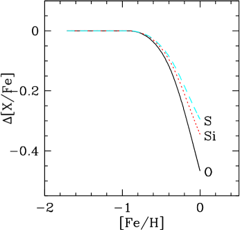
Figure 12.— Tracks in the $[{\rm X}/{\rm Fe}]-[{\rm Fe}/{\rm H}]$ plane for our fiducial model model parameters ($\eta=2.5$, $\tau_{*}=1\,{\rm Gyr}$, $\tau_{\rm sfh}=6\,{\rm Gyr}$, $\tau_{\rm Ia}=1.5\,{\rm Gyr}$, and $t_{D}=0.15\,{\rm Gyr}$) for oxygen (black solid), silicon (red dotted), and sulfur (cyan dashed), based on equation (109). Because silicon and sulfur have increasingly significant contributions from SNIa, they exhibit smaller drops in $[{\rm X}/{\rm Fe}]$ between the CCSN plateau ($\Delta[{\rm X}/{\rm Fe}]=0$ in this figure) and the late-time equilibrium.

In our calculations, we treat oxygen as an “idealized” $\alpha$-element, produced only by CCSNe, with a metallicity independent yield. Based on comparison to the more complete calculations in AWSJ, this idealization is good at the $\approx 0.05$ dex level. For a given star formation history, the evolution of $[{\rm O}/{\rm Fe}]$ relative to the early-time, CCSN plateau is governed by equation (42) and thus by the ratio $Z_{\rm Fe}^{\rm Ia}(t)/Z_{\rm Fe}^{\rm cc}(t)$. The value of $[{\rm O}/{\rm Fe}]$ at the plateau depends on CCSN yields and solar abundances as described by equation (44). As noted in §3.1, any other idealized $\alpha$-element should follow exactly the same track relative to its own early-time plateau. In particular, with the yields adopted by AWSJ, Mg production is also dominated almost entirely by CCSNe with metallicity-independent yield, so it should follow a nearly identical track to oxygen.

Moving up the periodic table, Si and S are $\alpha$-elements with increasingly significant predicted contributions from SNIa, though their production is still dominated by CCSN. For metallicity independent yields $m_{\rm X}^{\rm cc}$ and $m_{\rm X}^{\rm Ia}$ of an element X, the evolution of the relative abundance can be expressed in terms of the iron evolution and the relative yields:

$$\begin{split}{Z_{\rm X}(t)\over Z_{\rm Fe}(t)}&={Z_{\rm Fe}^{\rm cc}(t)m_{\rm X}^{\rm cc}/m_{\rm Fe}^{\rm cc}+Z_{\rm Fe}^{\rm Ia}(t)m_{\rm X}^{\rm Ia}/m_{\rm Fe}^{\rm Ia}\over Z_{\rm Fe}^{\rm cc}(t)+Z_{\rm Fe}^{\rm Ia}(t)}\\ &={m_{\rm X}^{\rm cc}\over m_{\rm Fe}^{\rm cc}}\times{1+{m_{\rm X}^{\rm Ia}/m_{\rm X}^{\rm cc}\over m_{\rm Fe}^{\rm Ia}/m_{\rm Fe}^{\rm cc}}Z_{\rm Fe}^{\rm Ia}(t)/Z_{\rm Fe}^{\rm cc}(t)\over 1+Z_{\rm Fe}^{\rm Ia}(t)/Z_{\rm Fe}^{\rm cc}(t)}~{}.\\ \end{split}$$ (108)

The plateau value of the abundance ratio is just $m_{\rm X}^{\rm cc}/m_{\rm Fe}^{\rm cc}$, so in combination with equation (42) we can write

$$\Delta[{\rm X}/{\rm Fe}]=\Delta[{\rm O}/{\rm Fe}]+\log_{\rm 10}\left[1+{m_{\rm X}^{\rm Ia}/m_{\rm X}^{\rm cc}\over m_{\rm Fe}^{\rm Ia}/m_{\rm Fe}^{\rm cc}}{Z_{\rm Fe}^{\rm Ia}(t)\over Z_{\rm Fe}^{\rm cc}(t)}\right]~{},$$ (109)

which as expected yields $\Delta[{\rm X}/{\rm Fe}]=\Delta[{\rm O}/{\rm Fe}]$ for any element with $m_{\rm X}^{\rm Ia}=0$, and yields $\Delta[{\rm X}/{\rm Fe}]=0$ for iron. Figure 12 shows relative abundance tracks for Si and S compared to the oxygen track, for the parameters of our fiducial model. Based on the IMF-integrated yields computed by AWSJ and the W70 model yield of Iwamoto et al. (1999), we have adopted $m_{\rm Si}^{\rm cc}=0.0013$ and $m_{\rm Si}^{\rm Ia}=0.24m_{\rm Si}^{\rm cc}=0.00031$ for silicon and $m_{\rm S}^{\rm cc}=0.00056$ and $m_{\rm S}^{\rm Ia}=0.36m_{\rm S}^{\rm cc}=0.00020$ for sulfur. Because of the increasing contribution of SNIa, the drops between the plateau and the equilibrium are successively smaller. For our adopted yields and the solar photospheric abundance values of Lodders (2003), the implied values of the plateau are $[{\rm O}/{\rm Fe}]_{\rm plateau}=+0.43$, $[{\rm Si}/{\rm Fe}]_{\rm plateau}=+0.26$, and $[{\rm S}/{\rm Fe}]_{\rm plateau}=+0.21$. If we used the Lodders (2003) recommended proto-solar abundances (corrected for diffusion) rather than photospheric abundances, then all of these values would drop by 0.07 dex.

Our prediction of similar $\Delta[{\rm X}/{\rm Fe}]$ for oxygen and magnesium and progressively lower values for Si and S is not in good agreement with observations. For example, the plateau values of $[{\rm Mg}/{\rm Fe}]$ and $[{\rm Si}/{\rm Fe}]$ found for solar neighborhood stars by Adibekyan et al. (2012) are approximately $+0.3$ and $+0.2$, but analyzing the same sample Bertran de Lis et al. (2015) find $[{\rm O}/{\rm Fe}]$ values for thick disk stars as high as $+0.5-0.8$. The compilation of $[{\rm S}/{\rm Fe}]$ values by Kacharov et al. (2015) (their Fig. 6), for individual stars and star clusters, suggests a plateau at $+0.4$. These discrepancies could reflect systematic errors in the observational abundances, which are difficult to place on a consistent scale across a wide range of $[{\rm Fe}/{\rm H}]$. Alternatively they could indicate a breakdown of our assumptions, particularly the assumption that the IMF-averaged yields are independent of metallicity. The yields of different elements are strongly dependent on stellar mass, so even if the yield at fixed stellar mass is metallicity independent, the IMF-averaged yield could vary if the IMF itself depends on metallicity or if the mass range of stars that explode as CCSNe changes with metallicity. Homogeneous analyses of large data sets such as APOGEE, Gaia-ESO, and GALAH should clarify whether there is indeed a discrepancy with observations to be explained.

5.5. Time-Dependent $\tau_{*}$

Perhaps the least desirable restriction of our analytic solutions is the requirement of constant SFE timescale $\tau_{*}$. While observations are consistent with a constant SFE for molecular gas in typical galaxies (Leroy et al., 2008), the non-linear form of the Kennicutt-Schmidt law (Schmidt, 1959; Kennicutt, 1998) implies that the SFE decreases with decreasing total (atomic + molecular) gas surface density. For one-zone models with declining star formation histories, therefore, a $\tau_{*}$ that increases with time would represent this situation more accurately.

Unfortunately constant $\tau_{*}$, or more precisely constant $\tau_{\rm dep}$, has a special place in allowing analytic solutions to our evolution equations. These generically have the form

$$\dot{M}(t)+{M(t)\over\tau_{\rm dep}}=mF(t)~{},$$ (110)

where the forcing function is $F(t)=\dot{M}_{*}(t)$ for CCSN products and $F(t)=\langle\dot{M}_{*}(t)\rangle_{\rm Ia}$ for SNIa products. Our analytic solution methods require analytic expressions for $\mu(t)=\exp[\int dt/\tau_{\rm dep}]$ and for $\int\mu(t)F(t)dt$. For constant $\tau_{\rm dep}$, $\int\mu(t)F(t)dt=\int e^{t/\tau_{\rm dep}}F(t)dt$ is analytic for interesting choices of $F(t)$, including ones involving an exponential DTD for SNIa. If $\tau_{\rm dep}$ is a function of $t$, then the integral is analytic only in special cases.

One such case is

$$\tau_{*}(t)=\tau_{*,0}(1+t/\tau_{\rm dep,0})$$ (111)

and thus

$$\tau_{\rm dep}(t)=\tau_{\rm dep,0}(1+t/\tau_{\rm dep,0})~{},$$ (112)

a depletion timescale that grows linearly from a starting value $\tau_{\rm dep,0}$, reaching double its initial value after $\tau_{\rm dep,0}$ and approaching $\tau_{\rm dep}(t)\approx t$ at late times. This case yields $\mu(t)=1+t/\tau_{\rm dep,0}$ and allows analytic solutions for both the oxygen mass and the iron mass as a function of time. We assume constant $\eta$ and $r$, so the gas mass at a given time is $M_{g}(t)=\dot{M}_{*}(t)\tau_{*}(t)=\dot{M}_{*}(t)\tau_{*,0}(1+t/\tau_{\rm dep,0})$. For an exponential star formation history, our usual solution methods yield, after some calculation,

$$\begin{split}Z_{\rm O}(t)=&{m_{\rm O}^{\rm cc}\over 1+\eta-r}\left({\tau_{\rm sfh}\over\tau_{\rm dep,0}}\right)\left(1+{t\over\tau_{\rm dep,0}}\right)^{-2}e^{t/\tau_{\rm sfh}}\times\\ &\left[\left(1+{\tau_{\rm sfh}\over\tau_{\rm dep,0}}\right)\left(1-e^{-t/\tau_{\rm sfh}}\right)-{t\over\tau_{\rm dep,0}}e^{-t/\tau_{\rm sfh}}\right]~{},\end{split}$$ (113)

and

$$\begin{split}Z_{\rm Fe}^{\rm Ia}(t)=&{m_{\rm Fe}^{\rm Ia}\over 1+\eta-r}\left({\bar{\tau}_{[{\rm Ia,sfh}]}\over\tau_{\rm Ia}}\right)\left(1+{t\over\tau_{\rm dep,0}}\right)^{-2}e^{t/\tau_{\rm sfh}}\times\\ &{1\over\tau_{\rm dep,0}}\Bigg{[}\left(1+{t\over\tau_{\rm dep,0}}\right)\left(\tau_{\rm Ia}e^{-\Delta t/\tau_{\rm Ia}}-\tau_{\rm sfh}e^{-\Delta t/\tau_{\rm sfh}}\right)+\\ &{1\over\tau_{\rm dep,0}}\left(\tau_{\rm Ia}^{2}e^{-\Delta t/\tau_{\rm Ia}}-\tau_{\rm sfh}^{2}e^{-\Delta t/\tau_{\rm sfh}}\right)-\\ &{1\over\tau_{\rm dep,0}}(\tau_{\rm Ia}-\tau_{\rm sfh})(t_{D}+\tau_{\rm dep,0}+\tau_{\rm Ia}+\tau_{\rm sfh})\Bigg{]}~{},\end{split}$$ (114)

where the latter expression is for $t>t_{D}$ only and $Z_{\rm Fe}^{\rm Ia}=0$ at $t\leq t_{D}$. These expressions are not particularly intuitive, and they do not asymptotically approach an equilibrium value like our expressions for constant $\tau_{\rm dep}$. Nonetheless, the behavior for realistic parameter values is not radically different from that of our previous solutions.

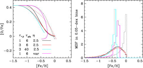
Figure 13.— Tracks in $[{\rm O}/{\rm Fe}]-[{\rm Fe}/{\rm H}]$ (left) and iron MDFs (right) for models with time-dependent SFE timescale $\tau_{*}$. Solid black and red curves show models with $\tau_{*}=\tau_{*,0}(1+t/\tau_{\rm dep,0})$ for $\tau_{*,0}=1$ and $3\,{\rm Gyr}$, respectively, and other parameters equal to those of our fiducial model. Dotted curves in the left panel show two corresponding models with constant $\tau_{*}=\tau_{*,0}$, and the dotted histogram in the right panel shows the MDF of the fiducial ($\tau_{*}=1\,{\rm Gyr}$) model. Cyan curves show a model with $\tau_{*,0}=3\,{\rm Gyr}$ and a long $\tau_{\rm sfh}$ that implies a nearly constant SFR. Magenta curves show a model in which $\eta(t)$ varies simultaneously with $\tau_{*}(t)$ in a way that keeps $\tau_{\rm dep}$ constant, following equations (115) and (116) with $q=2$ and $H(t)$ rising linearly from zero to one over 12.5 Gyr.

Figure 13 shows $[{\rm O}/{\rm Fe}]-[{\rm Fe}/{\rm H}]$ tracks and iron MDFs for three example cases. The first (black curves) has our fiducial model parameters but the time-dependent $\tau_{\rm dep}$ of equation (112), with $\tau_{\rm dep,0}=\tau_{*,0}/(1+\eta-r)=0.323\,{\rm Gyr}$. Compared to the constant $\tau_{*}$ case (dotted curves) the $[{\rm O}/{\rm Fe}]$ abundance ratio turns down at lower $[{\rm Fe}/{\rm H}]$ because $\tau_{*}$ has already grown by a factor $\sim 5$ by the time SNIa enrichment becomes important. At late times, the model track turns rightward to increasing $[{\rm Fe}/{\rm H}]$ at nearly solar $[{\rm O}/{\rm Fe}]$ because the depletion timescale starts to exceed the SFH timescale. The abundances at $t=12.5\,{\rm Gyr}$ are similar to those of the fiducial model. Increasing $\tau_{*,0}$ from $1\,{\rm Gyr}$ to $3\,{\rm Gyr}$ (red curves) shifts the knee to lower $[{\rm Fe}/{\rm H}]$ but makes little difference at late times, when the model has again approached $\tau_{\rm dep}\approx t$. The cyan curve shows the same case but with a nearly constant SFR ($\tau_{\rm sfh}=40\,{\rm Gyr}$), which eliminates the rightward turn in the $[{\rm O}/{\rm Fe}]-[{\rm Fe}/{\rm H}]$ track. Note that the SFE timescales of these models at $t=12.5\,{\rm Gyr}$ are $\tau_{*}\approx t(1+\eta-r)\approx 40\,{\rm Gyr}$, so the SFE at late times is extremely low.

MDFs for the two $\tau_{\rm sfh}=6\,{\rm Gyr}$ models qualitatively resemble the closed/leaky box form, which we found previously for “gas starved” models in which $\tau_{\rm sfh}$ is comparable to $\tau_{\rm dep}$. In both classes of models, the star formation rate declines substantially over a time interval in which the metallicity continues to grow, producing a smooth turnover rather than a sharp cutoff in $[{\rm Fe}/{\rm H}]$. The $\tau_{\rm sfh}=40\,{\rm Gyr}$ model, on the other hand, has a sharply peaked MDF, similar in form to that of our fiducial (constant $\tau_{\rm dep}$) model but shifted down in $[{\rm Fe}/{\rm H}]$ by 0.5-dex.

Because it is $\tau_{\rm dep}$ that enters our mass evolution equations, not $\tau_{*}$ directly, another way to allow time-dependent $\tau_{*}$ is to introduce a time-dependent $\eta$ that compensates to keep $\tau_{\rm dep}$ constant. For example, we can take

$$\tau_{*}(t)=\tau_{*,0}[1+qH(t)]~{},$$ (115)

where $q$ is a constant and $H(t)$ is a function that goes from 0 to 1 with an arbitrary time-dependence. If we simultaneously require

$$\begin{split}\eta(t)&=[1+qH(t)]{\tau_{*,0}/\tau_{\rm dep}}-1+r\\ &=\eta_{0}+qH(t)(1+\eta_{0}-r)\end{split}$$ (116)

then $\tau_{\rm dep}$ is constant and our standard solutions for $M_{\rm O}(t)$, $M_{\rm Fe}^{\rm cc}(t)$, and $M_{\rm Fe}^{\rm Ia}(t)$ apply. Compared to these standard solutions, however, the gas supply $M_{g}(t)=\tau_{*}(t)\dot{M}_{*}(t)$ at a given time is larger by a factor $\tau_{*}(t)/\tau_{*,0}=1+qH(t)$ and the abundances are lower by the same factor, with the abundance ratios unchanged. This behavior is pleasantly simple and holds for arbitrary $H(t)$, but it must be seen as the combined effect of raising $\tau_{*}$ and raising $\eta$, not either alone. Magenta curves in Figure 13 show a case in which $\tau_{*}$ rises linearly from $1\,{\rm Gyr}$ to $3\,{\rm Gyr}$ over the $12.5\,{\rm Gyr}$ span of the calculation. The $[{\rm O}/{\rm Fe}]-[{\rm Fe}/{\rm H}]$ track loops back to low $[{\rm Fe}/{\rm H}]$ after approaching solar $[{\rm O}/{\rm Fe}]$, similar to the model in Figure 9 for which a sudden increase in $\eta$ drives down the equilibrium abundance, though the increase here is steady rather than sudden. This model produces a sharply peaked MDF like that of our typical constant $\tau_{*}$ models, though the shape depends on the adopted $qH(t)$.

There may be other combinations of $\tau_{\rm dep}(t)$ and $\dot{M}_{*}(t)$ that yield analytic results for interesting illustrative cases, at least for oxgyen. Achieving analytic results for iron with a realistic SNIa DTD is harder because the $\mu(t)F(t)$ integral must still be analytic when the forcing function is $\langle\dot{M}_{*}(t)\rangle_{\rm Ia}$.

5.6. Generic sum of star formation histories

Returning to models with constant $\tau_{*}$ and $\eta$, we can combine results we have derived previously for constant, exponential, or linear-exponential star formation histories to derive solutions for more complex histories. Suppose that we have a solution to the generic evolution equation (110) for the forcing functions associated with a star formation history $\dot{M}_{*,1}(t)$ yielding a solution $M_{1}(t)$, where $M_{1}$ could refer to the oxygen, CCSN iron, or SNIa iron mass. Now consider a second solution $M_{2}(t)$ for a second star formation history $\dot{M}_{*,2}(t)$ with the same $\tau_{*}$ and $\eta$ (both constant in time). Linearity tells us that for the star formation history $\dot{M}_{*}(t)=\dot{M}_{*,1}(t)+\dot{M}_{*,2}(t)$ we can add the two forcing terms on the right hand side of equations (110) and get a solution with $M(t)=M_{1}(t)+M_{2}(t)$. Our solutions have the generic form $Z(t)=Z_{\rm eq}G(t)$ (e.g., equations 50, 53, 56, 58), implying $M(t)=Z_{\rm eq}G(t)\dot{M}_{*}(t)\tau_{*}$. To get the abundance for the combined star formation history we must add the two element masses and divide by the total gas mass $M_{g}(t)=\tau_{*}[\dot{M}_{*,1}(t)+\dot{M}_{*,2}(t)]$, obtaining

$$Z(t)={\dot{M}_{*,1}(t)Z_{\rm eq,1}G_{1}(t)+\dot{M}_{*,2}(t)Z_{\rm eq,2}G_{2}(t)\over\dot{M}_{*,1}(t)+\dot{M}_{*,2}(t)}~{}.$$ (117)

The solution for the combined star formation history is thus an average of the two individual solutions weighted by their contribution to the current star formation rate.

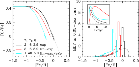
Figure 14.— Tracks in $[{\rm O}/{\rm Fe}]-[{\rm Fe}/{\rm H}]$ (left) and iron MDFs (right) for models in which the star formation history (SFH) is a sum of two components. All models have $\tau_{*}=1\,{\rm Gyr},$ $\tau_{\rm Ia}=1.5\,{\rm Gyr}$, $t_{D}=0.15\,{\rm Gyr}$. Solid black curves show an SFH that is the sum of two exponentials with timescales $\tau_{\rm sfh}=2\,{\rm Gyr}$ and $6\,{\rm Gyr}$. Red curves show an SFH with the same two timescales but a linear-exponential form. Cyan curves show the sum of a $1\,{\rm Gyr}$ linear-exponential and a nearly constant ($\tau_{\rm sfh}=40\,{\rm Gyr}$) exponential. Dotted black curves show the track and resulting MDF for a pure $2\,{\rm Gyr}$ exponential. The inset in the right panel shows the star formation histories. Values of $\eta$, indicated in the legend, have been chosen to maintain visual clarity.

Figure 14 shows $[{\rm O}/{\rm Fe}]-[{\rm Fe}/{\rm H}]$ tracks and iron MDFs for three examples of this class. In contrast to the models in Figure 9, all parameters are fixed throughout the evolution of each of these models, even though the star formation history is the sum of components with different timescales. The star formation histories themselves are shown in the inset of the right hand panel. In all cases we have chosen normalizations so that the integral (over $12.5\,{\rm Gyr}$) of the long timescale component is twice that of the short timescale component.

We have previously seen that for smooth star formation histories the shapes of tracks depend mainly on the outflow mass-loading and SFE timescale ($\eta$ and $\tau_{*}$), with little dependence on $\dot{M}_{*}(t)$, but the star formation history has a stronger impact on the MDF. Solid black curves in Figure 14 show a star formation history that is the sum of two exponentials with $\tau_{\rm sfh}=2\,{\rm Gyr}$ and $6\,{\rm Gyr}$, while the dotted curves show results for a single $\tau_{\rm sfh}=2\,{\rm Gyr}$ exponential for reference. The two models follow nearly identical tracks at early times, but the combined model stops at the near-solar equilibrium abundances characteristic of $\tau_{\rm sfh}=6\,{\rm Gyr}$ while the $\tau_{\rm sfh}=2\,{\rm Gyr}$ model continues on to sub-solar $[{\rm O}/{\rm Fe}]$ and super-solar $[{\rm Fe}/{\rm H}]$. The MDF of the $\tau_{\rm sfh}=2\,{\rm Gyr}$ model has the smooth cutoff characteristic of gas-starved models, expected because $\tau_{\rm sfh}<2\tau_{\rm Ia}$ (see §3.5). The combined model, on the other hand, has a sharply peaked MDF because of its longer $\tau_{\rm sfh}$ at late times.

Red curves show a similar case, but for linear-exponential histories instead of exponential histories. The overall behavior is similar to that of the combined exponential model, but the abundances are slightly lower because of the slower approach to equilibrium. (We have also increased $\eta$ from 2.5 to 3.0 to keep better visual separation of the models; results for $\eta=2.5$ are shifted slightly towards those of the combined exponential model.) Cyan curves show a more extreme example with a star formation history that begins with a sharply peaked, $\tau_{\rm sfh}=1\,{\rm Gyr}$, linear-exponential burst followed by a nearly constant SFR ($\tau_{\rm sfh}=40\,{\rm Gyr}$ exponential). Here we have adopted $\eta=5$ to keep visual separation from the other two models. The rapid early burst produces fast enrichment, and after reaching slightly sub-solar $[{\rm O}/{\rm Fe}]$ the model track loops back to the equilibrium abundances of the constant SFR model. The combination of two components with very different timescales makes a clear imprint on the MDF, which has a linear rise followed by a sharp peak.

6. Conclusions

Our main analytic results apply to one-zone models with metallicity-independent stellar yields and constant values of the governing parameters, in particular the star formation efficiency timescale $\tau_{*}$ and the outflow efficiency $\eta$. Crucially, our incorporation of a realistic DTD for Type Ia supernovae (either exponential or a sum of exponentials approximating a power law) allows us to compute the separate evolution of $\alpha$ and iron-peak elements. Realistic galaxies are more complex than these one-zone models, but our calculations provide a number of insights that are useful to understanding more general chemical evolution scenarios. The descriptions below continue to use oxygen as a representative $\alpha$ element, but our conclusions about oxygen also apply to other elements whose production is dominated by CCSNe and whose yields have weak metallicity dependence. We list our principal conclusions in several broad categories, then briefly discuss future applications of our results.

Equilibrium abundances

1. Under fairly general conditions, the abundances in a one-zone model with constant parameters evolve to an equilibrium in which the production of new metals is balanced by the combination of dilution and loss of metals to star formation and outflows. If the star formation rate is approximately constant, then oxygen approaches equilibrium on the gas depletion timescale $\tau_{\rm dep}=\tau_{*}/(1+\eta-r)$, while iron approaches equilibrium on the gas depletion or SNIa timescale ($\tau_{\rm Ia}\approx 1.5\,{\rm Gyr}$), whichever is longer.

2. At early times ($t\ll\tau_{\rm Ia}$) the $[{\rm O}/{\rm Fe}]$ ratio is determined by CCSN yields, $Z_{\rm O}/Z_{\rm Fe}=m_{\rm O}^{\rm cc}/m_{\rm Fe}^{\rm cc}$. For constant SFR, the equilibrium abundances at late times are $Z_{\rm O}=m_{\rm O}^{\rm cc}/(1+\eta-r)$ and $Z_{\rm Fe}=(m_{\rm Fe}^{\rm cc}+m_{\rm Fe}^{\rm Ia})/(1+\eta-r)$, with strong dependence on $\eta$. The equilibrium abundance ratio is $Z_{\rm O}/Z_{\rm Fe}=m_{\rm O}^{\rm cc}/(m_{\rm Fe}^{\rm cc}+m_{\rm Fe}^{\rm Ia})$, depending only on yields. Declining star formation histories lead to higher equilibrium abundances and lower equilibrium $[{\rm O}/{\rm Fe}]$.

3. Elevated $[{\rm O}/{\rm Fe}]$ ratios are a sign that the iron abundance, at least, has not yet reached equilibrium. Conversely, models with approximately solar or sub-solar $[{\rm O}/{\rm Fe}]$ are usually close to equilibrium in $[{\rm Fe}/{\rm H}]$. It is difficult to construct a model with constant parameters that shows significant increase in $[{\rm Fe}/{\rm H}]$ after reaching near-solar $[{\rm O}/{\rm Fe}]$; an extremely long gas depletion timescale is required.

4. A population can be low metallicity either because it has not had time to evolve to equilibrium or because the equilibrium abundance itself is low. Different factors may dominate in different situations, and both may be important in some cases. For example, gas rich dwarf galaxies may be metal poor because of low star formation efficiencies (large $\tau_{*}$), so that they remain below equilibrium, and dwarf spheroidal galaxies may have had their star formation truncated before reaching equilibrium. However, when star formation is vigorous the timescale for achieving equilibrium can be short, and many high-redshift galaxies may be low metallicity not because they are young but because they have high outflow rates that keep their equilibrium abundances low. Metallicity gradients in galaxies could arise from slower star formation (departure from equilibrium) or higher outflow efficiency (low equilibrium abundance) at larger radii. Mixing processes, not included in our models, may also play an important role in regulating gradients (e.g., Schönrich & Binney 2009; Bilitewski & Schönrich 2012; Pezzulli & Fraternali 2016).

Effect of star formation history

5. The behavior of one-zone models can be significantly different if the star formation rate is declining on a timescale $\tau_{\rm sfh}$ that is comparable to the depletion timescale $\tau_{\rm dep}$ or, for iron, to the SNIa timescale $\tau_{\rm Ia}$. A value of $\tau_{\rm sfh}\approx\tau_{\rm dep}$ arises when the system is “gas starved,” i.e., when the rate of gas accretion is much lower than the rate of gas depletion. In these cases the equilibrium abundances become large because metals are deposited in a rapidly declining gas supply, but the timescale to reach equilibrium becomes long.

6. Models with exponential ($\dot{M}_{*}\propto e^{-t/\tau_{\rm sfh}}$) and linear-exponential ($\dot{M}_{*}\propto te^{-t/\tau_{\rm sfh}}$) star formation histories have the same equilibrium abundances, but the early-time abundances are a factor of two lower for linear-exponential histories, and the approach to equilibrium is considerably slower. In either case, a more rapidly declining star formation history (shorter $\tau_{\rm sfh}$) leads to lower $[{\rm O}/{\rm Fe}]$ at equilibrium because the delayed SNIa enrichment, which comes from an earlier time when star formation was more rapid, is more important compared to ongoing CCSN enrichment.

Metallicity distribution functions

7. When $\tau_{\rm sfh}\gg\tau_{\rm dep}$ and $\tau_{\rm sfh}\gg\tau_{\rm Ia}$, a generic situation for a system with ongoing gas accretion, metallicity distribution functions (MDFs) are sharply peaked near the equilibrium abundance. The limiting case of constant SFR has $dN/dZ_{\rm O}\propto(1-Z_{\rm O}/Z_{\rm O,eq})^{-1}$ up to the current abundance $Z_{\rm O}(t)$. For oxygen, $\tau_{\rm sfh}=2\tau_{\rm dep}$ is a critical case with constant $dN/dZ_{\rm O}$, and shorter $\tau_{\rm sfh}$ produces declining $dN/dZ_{\rm O}$. The traditional “closed box” or “leaky box” scenarios represent the limiting case of no gas accretion, yielding $\tau_{\rm sfh}=\tau_{\rm dep}$, and this produces an exponential MDF $dN/dZ_{\rm O}\propto\exp[-Z_{\rm O}(1+\eta)/m_{\rm O}^{\rm cc}]$. However, these scenarios do not capture the typical behavior for star-forming systems with continuing accretion.

8. Similar considerations apply to iron MDFs, but here the relevant comparison timescale is usually $\tau_{\rm Ia}$ rather than $\tau_{\rm dep}$. A system with rapid accretion and rapid depletion can produce a rising $dN/dZ_{\rm O}$ and a declining $dN/dZ_{\rm Fe}$ if the timescales are such that $2\tau_{\rm dep}\lesssim\tau_{\rm sfh}\lesssim 2\tau_{\rm Ia}$. While the MDF shapes of $\alpha$-elements and iron-peak elements should typically be similar in form, cases where they differ can provide a distinctive diagnostic of enrichment timescales.

9. At early times ($t\ll\tau_{\rm dep}$ and $t\ll\tau_{\rm Ia}$) and low metallicities, exponential star formation histories produce constant $dN/dZ$ and linear-exponential star formation histories produce $dN/dZ\propto Z$, given our assumptions of constant $\tau_{*}$ and metallicity-independent yields. This behavior is sensitive to our assumption of instantaneous recycling of CCSN products.

Starbursts and sudden changes

10. Bursts of star formation, on the scale of an entire galaxy or of an individual molecular cloud or star-forming region, boost the rate of CCSN enrichment relative to SNIa enrichment. If the CCSN products are retained by the system, then a burst that converts a significant fraction of the available gas into stars can easily boost $[{\rm O}/{\rm Fe}]$ by 0.1-0.3 dex. The low observed scatter in $[{\rm O}/{\rm Fe}]$ at fixed $[{\rm Fe}/{\rm H}]$ (along either the “thick disk” or “thin disk” sequences) sets limits on the importance of this time-varying enrichment effect. In typical molecular clouds, it is probably small because of low conversion efficiency, and perhaps because the CCSN metals are lost before they can be incorporated into new stars. However, molecular clouds vary in their properties, and occasional systems that form stars efficiently and retain their metals could be a source of rare $\alpha$-enhanced stars at intermediate ages (Martig et al., 2015; Chiappini et al., 2015; Haywood et al., 2015). Bursty star formation histories in dwarf galaxies could have a significant impact on their $[{\rm O}/{\rm Fe}]$ distributions, relative to smooth star formation histories with the same time-averaged behavior (Gilmore & Wyse, 1991).

11. A rapid change from efficient star formation (short $\tau_{*}$) to inefficient star formation (long $\tau_{*}$) can lead to a substantial drop in $[{\rm O}/{\rm Fe}]$, as iron deposition exceeds oxygen deposition. Conversely, a rapid change from low efficiency to high efficiency leads to a temporary boost in $[{\rm O}/{\rm Fe}]$.

12. One can produce an evolutionary sequence that has increasing $[{\rm Fe}/{\rm H}]$ at low $[{\rm O}/{\rm Fe}]$ by decreasing $\eta$, and thus raising the equilibrium abundance itself, after the population has already evolved to an initial equilibrium. Alternatively, by increasing the outflow efficiency at late times, one can construct an evolutionary track that reaches solar $[{\rm O}/{\rm Fe}]$ and $[{\rm Fe}/{\rm H}]$ and then moves backward to lower $[{\rm Fe}/{\rm H}]$ at constant $[{\rm O}/{\rm Fe}]$ because of the reduction in equilibrium abundance. This backward evolution scenario allows a single evolutionary track to produce a bimodal distribution in the $[{\rm O}/{\rm Fe}]$-$[{\rm Fe}/{\rm H}]$ plane.

Intermediate elements

13. In any one-zone model, all “idealized” $\alpha$ elements, by which we mean elements produced entirely by CCSNe with a metallicity-independent yield, follow the same track in $[{\rm X}/{\rm Fe}]$ vs. $[{\rm Fe}/{\rm H}]$, described by equation (42). In particular, the drop between the CCSN plateau and the eventual equilibrium $[{\rm X}/{\rm Fe}]$ is the same for all such elements. When an observed element does not show this behavior, it indicates that there is another significant source (SNIa or AGB production), or that the IMF-averaged yield is metallicity dependent, or that the observational estimates of the abundance are systematically biased; any one of these would be an interesting conclusion. Elements like sulfur that have a subdominant but non-negligible contribution from SNIa should show intermediate behavior, as described by equation (109). Detailed comparisons of the $[{\rm X}/{\rm Fe}]$ tracks of different $\alpha$-elements should provide significant insights on their production mechanisms. Even when yields have weak metallicity dependence at a fixed stellar mass, the IMF-averaged yield could change with metallicity either because the IMF itself changes or because the mass ranges of stars that explode as CCSNe (instead of collapsing to black holes) change with metallicity.

Applications

Beyond these insights, we expect our analytic solutions to have significant practical utility for modeling observations. The key equations are (50), (52), (53) for oxygen, CCSN iron, and SNIa iron evolution with an exponential star formation history and the corresponding equations (56), (57), and (58) for linear-exponential star formation histories. Section 4.2 and §5 describe a variety of ways to extend these results, including more complex star formation histories, double-exponential DTDs for SNIa, models with discontinuous parameter changes, and $\alpha$-elements with significant SNIa contributions. Analytic solutions enable rapid explorations of parameter space, zeroing in on regions of observational or physical interest that merit detailed numerical modeling. They are useful for characterizing degeneracies among parameters, to better understand whether a fit to data is unique or one among many. In more quantitative terms, their speed of calculation makes them useful for statistical modeling of data sets via likelihood methods, Markov Chain Monte Carlo sampling, or related techniques (e.g., Kirby et al. 2013). While most systems of interest are more complicated than a one-zone model, some may be usefully approximated by mixtures of one-zone models, or by a one-zone model whose geometry and kinematics change over time to represent heating or contraction.

These models are aimed principally at the interpretation of resolved stellar populations with star-by-star abundance measurements. They may also be useful for modeling gas phase abundances and connecting them to underlying stellar populations, an application of growing importance in the era of large IFU surveys such as CALIFA (Sánchez et al., 2012), SAMI (Croom et al., 2012), and MaNGA (Bundy et al., 2015). They can also be incorporated into population synthesis models of galactic spectral energy distributions, tying a distribution of stellar metallicities to an inferred history of star formation. They can be used as an approximate tool for post-processing numerical simulations to make chemical evolution predictions in simulations that do not explicitly track multi-element enrichment.

The high-fiber revolution that transformed the study of large scale structure is now transforming our knowledge of the multi-element distributions of stellar populations in the Milky Way and its neighbors. These rich data sets, often augmented by phase space information from astrometry and age information from asteroseismology, offer many clues to the history of our Galaxy. One of the challenges in interpreting these clues is evaluating the uniqueness of successful models, especially in light of systematic uncertainties in element yields and the observed abundances themselves. Flexible approximate models can play a valuable role in mapping out the variety of routes to a given final state and identifying the observational features that may best distinguish competing scenarios.

Appendix B provides a step-by-step guide to using our analytic results for computing enrichment histories, $[\alpha/{\rm Fe}]$ tracks, and MDFs.

We are grateful to Ralph Schönrich and Jennifer Johnson for several years worth of invaluable education about chemical evolution modeling. We thank Evan Kirby, Molly Peeples, Ralph Schönrich, and Philipp Kempski for numerous helpful comments on an earlier version of the manuscript. This work was supported by NSF grant AST-1211853.

Appendix A A. SNIa Enrichment

Define the SNIa rate $R(\nu)$ such that $R(\nu)d\nu$ is the number of SNIa per unit mass of stars formed that explode in the time interval $\nu\rightarrow\nu+d\nu$ following the formation of a population at time $\nu=0$. The units of $R(\nu)$ are $M_{\odot}^{-1}\,{\rm yr}^{-1}$. We use the variable $\nu$ to avoid confusion with time $t$ in a continuously forming stellar population.

As already noted in equation (2), we define the population averaged SNIa iron yield to be

$$m_{\rm Fe}^{\rm Ia}\equiv K_{\rm Fe}^{\rm Ia}\int_{0}^{\infty}R(\nu)d\nu~{},$$ (A1)

where $K_{\rm Fe}^{\rm Ia}$ is the mean mass of iron ejected per SNIa. This expression implicitly assumes that the integral converges to a finite value, which it does for an exponential DTD. For a form of the DTD for which the integral does not converge, such as $R(\nu)\propto\nu^{-1}$, one can simply cut off the integral at some time larger than the age of the universe, with no loss of generality in our equations.

For a star formation history $\dot{M}_{*}(t)$, the rate at which SNIa inject iron to the ISM is

$$\dot{M}_{\rm Fe}^{\rm Ia}(t)=K_{\rm Fe}^{\rm Ia}\int_{0}^{t}\dot{M}_{*}(t^{\prime})R(t-t^{\prime})dt^{\prime}=m_{\rm Fe}^{\rm Ia}\langle\dot{M}_{*}(t)\rangle_{\rm Ia}$$ (A2)

where $\langle\dot{M}_{*}(t)\rangle_{\rm Ia}$ is given by equation (A4). For a DTD that is zero prior to $t_{D}$ and exponential thereafter, $R(\nu)=R_{0}e^{-(\nu-t_{D})/\tau_{\rm Ia}}$, implying

$$\int_{0}^{\infty}R(\nu)d\nu=R_{0}\tau_{\rm Ia}$$ (A3)

and

$$\langle\dot{M}_{*}(t)\rangle_{\rm Ia}=\tau_{\rm Ia}^{-1}\int_{0}^{t-t_{D}}\dot{M}_{*}(t^{\prime})e^{-(t-t^{\prime}-t_{D})/\tau_{\rm Ia}}dt^{\prime}~{},$$ (A4)

where the upper limit is set to $t-t_{D}$ because the SNIa rate is zero for more recent star formation. For the case of a constant SFR, evaluating this integral yields

$$\langle\dot{M}_{*}(t)\rangle_{\rm Ia}=\dot{M}_{*}\left[1-e^{-\Delta t/\tau_{\rm Ia}}\right]~{},\quad{\rm constant~{}SFR}~{},$$ (A5)

with $\Delta t\equiv t-t_{D}$.

For an exponentially declining star formation history, $\dot{M}_{*}(t)=\dot{M}_{*,0}e^{-t/\tau_{\rm sfh}}$,

$$\langle\dot{M}_{*}(t)\rangle_{\rm Ia}=\dot{M}_{*,0}\tau_{\rm Ia}^{-1}\int_{0}^{t-t_{D}}e^{-t^{\prime}/\tau_{\rm sfh}}e^{-(\Delta t-t^{\prime})/\tau_{\rm Ia}}dt^{\prime}~{}.$$ (A6)

Since $e^{-\Delta t/\tau_{\rm Ia}}$ is independent of $t^{\prime}$ it can be factored out of the integral, yielding

$$\langle\dot{M}_{*}(t)\rangle_{\rm Ia}=\dot{M}_{*,0}\tau_{\rm Ia}^{-1}e^{-\Delta t/\tau_{\rm Ia}}\int_{0}^{t-t_{D}}e^{-t^{\prime}/\tau_{\rm sfh}}e^{t^{\prime}/\tau_{\rm Ia}}dt^{\prime}~{}.$$ (A7)

Using the notation (23) allows the integrand to be written $e^{t^{\prime}/\bar{\tau}_{[{\rm Ia,sfh}]}}$, and evaluating the integral yields

$$\langle\dot{M}_{*}(t)\rangle_{\rm Ia} = \dot{M}_{*,0}\left({\bar{\tau}_{[{\rm Ia,sfh}]}\over\tau_{\rm Ia}}\right)e^{-\Delta t/\tau_{\rm Ia}}\left[e^{\Delta t/\bar{\tau}_{[{\rm Ia,sfh}]}}-1\right]$$ (A8)

$$= \dot{M}_{*,0}\left({\bar{\tau}_{[{\rm Ia,sfh}]}\over\tau_{\rm Ia}}\right)\left[e^{-\Delta t/\tau_{\rm sfh}}-e^{-\Delta t/\tau_{\rm Ia}}\right]~{},$$ (A9)

where the second equality uses $\tau_{\rm Ia}^{-1}-\bar{\tau}_{[{\rm Ia,sfh}]}^{-1}=\tau_{\rm sfh}^{-1}$. From here we can factor out $e^{-\Delta t/\tau_{\rm sfh}}$ and use the substitution $\dot{M}_{*,0}e^{-\Delta t/\tau_{\rm sfh}}=\dot{M}_{*}(t)e^{t_{D}/\tau_{\rm sfh}}$ to write

$$\langle\dot{M}_{*}(t)\rangle_{\rm Ia}=\dot{M}_{*}(t)e^{t_{D}/\tau_{\rm sfh}}{\bar{\tau}_{[{\rm Ia,sfh}]}\over\tau_{\rm Ia}}\left[1-e^{-\Delta t/\bar{\tau}_{[{\rm Ia,sfh}]}}\right]~{},\quad{\rm exponential~{}SFH}~{},$$ (A10)

which in turn leads to equation (21).

This example illustrates several of the features that arise throughout our calculations, in particular the appearance and behavior of harmonic difference timescales. While $\bar{\tau}_{[{\rm Ia,sfh}]}$ can be positive or negative, the factor in $[...]$ always has the same sign as $\bar{\tau}_{[{\rm Ia,sfh}]}$, forcing $\langle\dot{M}_{*}(t)\rangle_{\rm Ia}$ to be positive. Note that for $\tau_{\rm Ia}\approx\tau_{\rm sfh}$, and thus large $\bar{\tau}_{[{\rm Ia,sfh}]}$, Taylor-expanding the exponential yields

$$\langle\dot{M}_{*}(t)\rangle_{\rm Ia}=\dot{M}_{*}(t)e^{t_{D}/\tau_{\rm sfh}}{\Delta t\over\tau_{\rm Ia}}~{}.$$ (A11)

Thus, the result does not diverge even as $\tau_{\rm Ia}\rightarrow\tau_{\rm sfh}$ and $\bar{\tau}_{[{\rm Ia,sfh}]}\rightarrow\infty$.

For $\dot{M}_{*}(t)\propto te^{-t/\tau_{\rm sfh}}$ the procedure is similar, but the integral that enters is $\int xe^{x}dx$ rather than $\int e^{x}dx$, leading to combinations of linear and exponential terms. The result can be expressed

$${\langle\dot{M}_{*}\rangle_{\rm Ia}\over\dot{M}_{*}}=e^{t_{D}/\tau_{\rm sfh}}\left({\bar{\tau}_{[{\rm Ia,sfh}]}\over\tau_{\rm Ia}}\right){\bar{\tau}_{[{\rm Ia,sfh}]}\over t}\left[{\Delta t\over\bar{\tau}_{[{\rm Ia,sfh}]}}+e^{-\Delta t/\bar{\tau}_{[{\rm Ia,sfh}]}}-1\right]~{},\quad\hbox{{\rm linear-exponential~{}SFH}}.$$ (A12)

Appendix B B. A User’s Guide

Our analytic results provide a flexible tool for computing $[{\rm O}/{\rm Fe}]-[{\rm Fe}/{\rm H}]$ tracks, age-metallicity and age-$[{\rm O}/{\rm Fe}]$ relations, and MDFs for comparisons to observational data or as inputs for population synthesis or theoretical models. Here we provide a step-by-step guide for such calculations, which can be implemented easily in a plotting package such as sm, or any programming language. We begin with the most straightforward case of a single-exponential SNIa DTD and model parameters $\eta$, $\tau_{*}$, and $\tau_{\rm sfh}$ that are fixed throughout the evolution. We then summarize how to implement the two-exponential DTDs of §5.1, which approximate a $t^{-1.1}$ power-law, and how to implement models with sudden parameter changes, like those of §4.

Set the physical parameters

• Choose values for the supernova yield parameters $m_{\rm O}^{\rm cc}$, $m_{\rm Fe}^{\rm cc}$, and $m_{\rm Fe}^{\rm Ia}$. The default values listed in Table 1 are reasonable choices, based on the assumptions described in §2.2.

• Choose a value of the mass recycling parameter $r$. Our fiducial value $r=0.4$ is a good choice for a Kroupa IMF, and results are only weakly sensitive to this parameter.

• Choose values for the solar oxygen and iron abundance. To convert from the conventional shifted number density scale $x_{i}\equiv 12+\log(X_{i}/H)$ to mass fractions use

  $$\log Z_{{\rm O},\odot} = (x_{\rm O}-12)+\log(16)+\log(0.71)=-2.25+(x_{\rm O}-8.69)~{},$$ (B1)

  $$\log Z_{{\rm Fe},\odot} = (x_{\rm Fe}-12)+\log(55.85)+\log(0.71)=-2.93+(x_{\rm Fe}-7.47)~{},$$ (B2)

  where we have adopted a solar hydrogen mass fraction of 0.71 and an atomic weight of 55.85 for iron.

• Choose values for the SNIa DTD timescale $\tau_{\rm Ia}$ and the minimum delay time $t_{D}$. Our fiducial values are $\tau_{\rm Ia}=1.5\,{\rm Gyr}$ and $t_{D}=0.15\,{\rm Gyr}$.

Choose model parameters and compute equilibrium abundances

• Specify values of the mass-loading parameter $\eta$, the star formation efficiency timescale $\tau_{*}$, and the $e$-folding timescale for the star formation rate, $\tau_{\rm sfh}$.

• Calculate the depletion timescale $\tau_{\rm dep}=\tau_{*}/(1+\eta-r)$. Calculate the harmonic difference timescales $\bar{\tau}_{[{\rm dep,sfh}]}$, $\bar{\tau}_{[{\rm dep,Ia}]}$, and $\bar{\tau}_{[{\rm Ia,sfh}]}$ from equation (23). If you will be exploring many parameter values, it may be useful to multiply $\tau_{*}$, $\tau_{\rm sfh}$, and $\tau_{\rm Ia}$ by numbers that are very slightly different from one to avoid exact equalities that lead to undefined values of the harmonic difference timescales. As discussed in the text, abundance results are convergent and physical even near limits where one of these timescales diverges.

• Compute the equilibrium abundances $Z_{\rm O,eq}$, $Z^{\rm cc}_{\rm Fe,eq}$, and $Z^{\rm Ia}_{\rm Fe,eq}$ from equations (28)-(30).

Compute time evolution and MDF

• Choose an exponential or linear-exponential star formation history. By setting $\tau_{\rm sfh}$ to a large value, one can also use these cases to approximate a constant SFR or linearly rising SFR, respectively.

• Compute $Z_{\rm O}(t)$ and $Z_{\rm Fe}(t)=Z_{\rm Fe}^{\rm cc}(t)+Z_{\rm Fe}^{\rm Ia}(t)$ using equations (50), (52), and (53) for an exponential SFH or equations (56), (57), and (58) for a linear-exponential SFH. These can be converted to $[{\rm O}/{\rm H}]=\log(Z_{\rm O}/Z_{{\rm O},\odot})$, $[{\rm Fe}/{\rm H}]=\log(Z_{\rm Fe}/Z_{{\rm Fe},\odot})$, and $[{\rm O}/{\rm Fe}]=[{\rm O}/{\rm H}]-[{\rm Fe}/{\rm H}]$.

• To compute an iron MDF, first choose bins for $[{\rm Fe}/{\rm H}]$. Then compute $Z_{\rm Fe}(t)$ with a constant time spacing and add a quantity proportional to $\dot{M}_{*}(t)$, and hence to the number of stars formed during the time interval, to the $[{\rm Fe}/{\rm H}]$ bin in which $Z_{\rm Fe}(t)$ falls. The resulting histogram can be multiplied by a constant to normalize it to unit integral. Short time spacings (e.g., $0.002\,{\rm Gyr}$) may be necessary to get accurate and smooth results at low metallicity.

• Distributions of $[{\rm O}/{\rm Fe}]$ and $[{\rm O}/{\rm H}]$ can be computed in the same way as the iron MDF. Equations (62) and (63) provide analytic forms for the oxygen MDF for a constant or exponential SFH, respectively.

• To model a more general star formation history that is a sum of exponentials and/or linear-exponentials, follow equation (117).

Two-exponential DTD

To approximate a $t^{-1.1}$ DTD with a minimum delay time of $t_{D}=0.15\,{\rm Gyr}$, we recommend a sum of two exponential DTDs with timescales of $\tau=0.5\,{\rm Gyr}$ and $5\,{\rm Gyr}$. Proceed as before, but compute and add two values of $Z_{\rm Fe}^{\rm Ia}(t)$ to get the total SNIa iron contribution, multiplying the value of $m_{\rm Fe}^{\rm Ia}$ by $(0.478,0.522)$ for $\tau=(0.5,5)$ so that each exponential is normalized to produce half of the SNIa iron over $12.5\,{\rm Gyr}$ (see footnote in §5.1). Note that the harmonic difference timescales and $Z^{\rm Ia}_{\rm Fe,eq}$ must be computed separately for the two exponentials.

For a minimum delay time of $t_{D}=0.05\,{\rm Gyr}$, we recommend a sum of two exponential DTDs with $\tau=(0.25,3.5)\,{\rm Gyr}$ and $m_{\rm Fe}^{\rm Ia}$ multiplied by $(0.493,0.507)$. Experimentation along the lines illustrated in Figure 10 can be carried out to find exponential combinations for other minimum delay times or other functional forms of the DTD.

Sudden Parameter Changes

Section 4 describes how to calculate a model in which parameters ($\tau_{*}$, $\eta$, $\tau_{\rm sfh}$) change from one value to another at a transition time $t_{c}$. For times $t<t_{c}$, proceed as before, and record the values of $Z_{\rm O}(t_{c})$ and $Z_{\rm Fe}(t_{c})$ for subsequent use. For times $t>t_{c}$, compute quantities $\tau_{\rm dep2}$, $\bar{\tau}_{[{\rm Ia,sfh2}]}$, $\bar{\tau}_{[{\rm dep2,sfh2}]}$, and $\bar{\tau}_{[{\rm dep2,Ia}]}$ using the the post-$t_{c}$ parameter values. Compute the corresponding equilibrium abundances. Defining $t_{2}=t-t_{c}$, compute the contributions $Z_{\rm O,1}(t_{2})$ and $Z_{\rm O,2}(t_{2})$ from equations (81) and (82) and sum them to get $Z_{\rm O}(t_{2})$. For iron, compute and sum the values of $Z_{\rm Fe,1}(t_{2})$, $Z_{\rm Fe,2}(t_{2})$, and $Z_{\rm Fe,3}(t_{2})$ from equations (84), (85), and (91), respectively.

References

- Adibekyan et al. (2012) Adibekyan, V. Z., Sousa, S. G., Santos, N. C., et al. 2012, A&A, 545, A32
- Belfiore et al. (2016) Belfiore, F., Maiolino, R., & Bothwell, M. 2016, MNRAS, 455, 1218
- Bertran de Lis et al. (2015) Bertran de Lis, S., Delgado Mena, E., Adibekyan, V. Z., Santos, N. C., & Sousa, S. G. 2015, A&A, 576, A89
- Bilitewski & Schönrich (2012) Bilitewski, T., & Schönrich, R. 2012, MNRAS, 426, 2266
- Binney & Merrifield (1998) Binney, J., & Merrifield, M. 1998, Galactic Astronomy
- Bird et al. (2012) Bird, J. C., Kazantzidis, S., & Weinberg, D. H. 2012, MNRAS, 420, 913
- Bundy et al. (2015) Bundy, K., Bershady, M. A., Law, D. R., et al. 2015, ApJ, 798, 7
- Chiappini et al. (1997) Chiappini, C., Matteucci, F., & Gratton, R. 1997, ApJ, 477, 765
- Chiappini et al. (2015) Chiappini, C., Anders, F., Rodrigues, T. S., et al. 2015, A&A, 576, L12
- Chieffi & Limongi (2004) Chieffi, A., & Limongi, M. 2004, ApJ, 608, 405
- Colavitti et al. (2008) Colavitti, E., Matteucci, F., & Murante, G. 2008, A&A, 483, 401
- Croom et al. (2012) Croom, S. M., Lawrence, J. S., Bland-Hawthorn, J., et al. 2012, MNRAS, 421, 872
- Dalcanton (2007) Dalcanton, J. J. 2007, ApJ, 658, 941
- De Silva et al. (2015) De Silva, G. M., Freeman, K. C., Bland-Hawthorn, J., et al. 2015, MNRAS, 449, 2604
- Edvardsson et al. (1993) Edvardsson, B., Andersen, J., Gustafsson, B., et al. 1993, A&A, 275, 101
- Ferrara et al. (2005) Ferrara, A., Scannapieco, E., & Bergeron, J. 2005, ApJ, 634, L37
- Finlator & Davé (2008) Finlator, K., & Davé, R. 2008, MNRAS, 385, 2181
- Fraternali & Binney (2008) Fraternali, F., & Binney, J. J. 2008, MNRAS, 386, 935
- Gallazzi et al. (2008) Gallazzi, A., Brinchmann, J., Charlot, S., & White, S. D. M. 2008, MNRAS, 383, 1439
- Gilmore & Wyse (1991) Gilmore, G., & Wyse, R. F. G. 1991, ApJ, 367, L55
- Gilmore et al. (2012) Gilmore, G., Randich, S., Asplund, M., et al. 2012, The Messenger, 147, 25
- Greggio (2005) Greggio, L. 2005, A&A, 441, 1055
- Hartwick (1976) Hartwick, F. D. A. 1976, ApJ, 209, 418
- Hayden et al. (2015) Hayden, M. R., Bovy, J., Holtzman, J. A., et al. 2015, ApJ, 808, 132
- Haywood et al. (2015) Haywood, M., Di Matteo, P., Snaith, O., & Lehnert, M. D. 2015, A&A, 579, A5
- Iwamoto et al. (1999) Iwamoto, K., Brachwitz, F., Nomoto, K., et al. 1999, ApJS, 125, 439
- Kacharov et al. (2015) Kacharov, N., Koch, A., Caffau, E., & Sbordone, L. 2015, ArXiv e-prints, arXiv:1503.02691
- Kalirai et al. (2008) Kalirai, J. S., Hansen, B. M. S., Kelson, D. D., et al. 2008, ApJ, 676, 594
- Kennicutt (1998) Kennicutt, Jr., R. C. 1998, ApJ, 498, 541
- Kirby et al. (2013) Kirby, E. N., Cohen, J. G., Guhathakurta, P., et al. 2013, ApJ, 779, 102
- Kroupa (2001) Kroupa, P. 2001, MNRAS, 322, 231
- Larson (1972) Larson, R. B. 1972, Nature Physical Science, 236, 7
- Lee et al. (2010) Lee, S.-K., Ferguson, H. C., Somerville, R. S., Wiklind, T., & Giavalisco, M. 2010, ApJ, 725, 1644
- Leroy et al. (2008) Leroy, A. K., Walter, F., Brinks, E., et al. 2008, AJ, 136, 2782
- Lilly et al. (2013) Lilly, S. J., Carollo, C. M., Pipino, A., Renzini, A., & Peng, Y. 2013, ApJ, 772, 119
- Limongi & Chieffi (2006) Limongi, M., & Chieffi, A. 2006, ApJ, 647, 483
- Lodders (2003) Lodders, K. 2003, ApJ, 591, 1220
- Lynden-Bell (1975) Lynden-Bell, D. 1975, Vistas in Astronomy, 19, 299
- Majewski et al. (2016) Majewski, S. R., Schiavon, R. P., Frinchaboy, P. M., et al. 2016, ArXiv e-prints, arXiv:1509.05420
- Maoz & Mannucci (2012) Maoz, D., & Mannucci, F. 2012, PASA, 29, 447
- Maoz et al. (2012) Maoz, D., Mannucci, F., & Brandt, T. D. 2012, MNRAS, 426, 3282
- Martig et al. (2015) Martig, M., Rix, H.-W., Silva Aguirre, V., et al. 2015, MNRAS, 451, 2230
- Matteucci (2001) Matteucci, F., ed. 2001, Astrophysics and Space Science Library, Vol. 253, The chemical evolution of the Galaxy
- Matteucci (2012) Matteucci, F. 2012, Chemical Evolution of Galaxies, doi:10.1007/978-3-642-22491-1
- Matteucci & Francois (1989) Matteucci, F., & Francois, P. 1989, MNRAS, 239, 885
- Murray (2011) Murray, N. 2011, ApJ, 729, 133
- Nidever et al. (2014) Nidever, D. L., Bovy, J., Bird, J. C., et al. 2014, ApJ, 796, 38
- Pagel (1997) Pagel, B. E. J. 1997, Nucleosynthesis and Chemical Evolution of Galaxies, 392
- Pagel & Patchett (1975) Pagel, B. E. J., & Patchett, B. E. 1975, MNRAS, 172, 13
- Peeples & Shankar (2011) Peeples, M. S., & Shankar, F. 2011, MNRAS, 417, 2962
- Peeples et al. (2014) Peeples, M. S., Werk, J. K., Tumlinson, J., et al. 2014, ApJ, 786, 54
- Pezzulli & Fraternali (2016) Pezzulli, G., & Fraternali, F. 2016, MNRAS, 455, 2308
- Qian & Wasserburg (2012) Qian, Y.-Z., & Wasserburg, G. J. 2012, Proceedings of the National Academy of Science, 109, 4750
- Ramírez et al. (2013) Ramírez, I., Allende Prieto, C., & Lambert, D. L. 2013, ApJ, 764, 78
- Recchi et al. (2008) Recchi, S., Spitoni, E., Matteucci, F., & Lanfranchi, G. A. 2008, A&A, 489, 555
- Roškar et al. (2008) Roškar, R., Debattista, V. P., Quinn, T. R., Stinson, G. S., & Wadsley, J. 2008, ApJ, 684, L79
- Sánchez et al. (2012) Sánchez, S. F., Kennicutt, R. C., Gil de Paz, A., et al. 2012, A&A, 538, A8
- Scannapieco & Bildsten (2005) Scannapieco, E., & Bildsten, L. 2005, ApJ, 629, L85
- Schmidt (1959) Schmidt, M. 1959, ApJ, 129, 243
- Schmidt (1963) —. 1963, ApJ, 137, 758
- Schönrich & Binney (2009) Schönrich, R., & Binney, J. 2009, MNRAS, 396, 203
- Sellwood & Binney (2002) Sellwood, J. A., & Binney, J. J. 2002, MNRAS, 336, 785
- Simha et al. (2014) Simha, V., Weinberg, D. H., Conroy, C., et al. 2014, ArXiv e-prints, arXiv:1404.0402
- Spitoni (2015) Spitoni, E. 2015, MNRAS, 451, 1090
- Spitoni & Matteucci (2011) Spitoni, E., & Matteucci, F. 2011, A&A, 531, A72
- Talbot & Arnett (1971) Talbot, Jr., R. J., & Arnett, W. D. 1971, ApJ, 170, 409
- Tinsley (1975) Tinsley, B. M. 1975, ApJ, 197, 159
- Tinsley (1980) —. 1980, Fund. Cosmic Phys., 5, 287
- Tinsley & Larson (1978) Tinsley, B. M., & Larson, R. B. 1978, ApJ, 221, 554
- Weisz et al. (2014) Weisz, D. R., Dolphin, A. E., Skillman, E. D., et al. 2014, ApJ, 789, 147
- Wielen et al. (1996) Wielen, R., Fuchs, B., & Dettbarn, C. 1996, A&A, 314
- Yanny et al. (2009) Yanny, B., Rockosi, C., Newberg, H. J., et al. 2009, AJ, 137, 4377
- Zahid et al. (2012) Zahid, H. J., Dima, G. I., Kewley, L. J., Erb, D. K., & Davé, R. 2012, ApJ, 757, 54