On the Deuterium-to-Hydrogen Ratio of the Interstellar Medium

Abstract

Observational studies show that the global deuterium-to-hydrogen ratio $({\rm D}/{\rm H})$ in the local interstellar medium (ISM) is about 90% of the primordial ratio predicted by big bang nucleosynthesis. The high $({\rm D}/{\rm H})_{\rm ISM}$ implies that only a small fraction of interstellar gas has been processed through stars, which destroy any deuterium they are born with. Using analytic arguments for one-zone chemical evolution models that include accretion and outflow, I show that the deuterium abundance is tightly coupled to the abundance of core collapse supernova (CCSN) elements such as oxygen. These models predict that the ratio of the ISM deuterium abundance to the primordial abundance is $X_{\rm D}/X_{\rm D}^{\rm P}\approx(1+rZ_{\rm O}/m_{\rm O}^{\rm cc})^{-1}$, where $r$ is the recycling fraction, $Z_{\rm O}$ is the ISM oxygen mass fraction, and $m_{\rm O}^{\rm cc}$ is the population averaged CCSN yield of oxygen. Using values $r=0.4$ and $m_{\rm O}^{\rm cc}=0.015$ appropriate to a Kroupa (2001) initial mass function and recent CCSN yield calculations, solar oxygen abundance corresponds to $X_{\rm D}/X_{\rm D}^{\rm P}\approx 0.87$, consistent with observations. This approximation is accurate for a wide range of parameter values, and physical arguments and numerical tests suggest that it should remain accurate for more complex chemical evolution models. The good agreement with the upper range of observed $({\rm D}/{\rm H})_{\rm ISM}$ values supports the long-standing suggestion that sightline-to-sightline variations of deuterium are a consequence of dust depletion, rather than a low global $({\rm D}/{\rm H})_{\rm ISM}$ enhanced by localized accretion of primordial composition gas. This agreement limits deviations from conventional yield and recycling values, including models in which most high mass stars collapse to form black holes without expelling their oxygen in supernovae, and it implies that Galactic outflows eject ISM hydrogen as efficiently as they eject CCSN metals.

1. Introduction

Most of the atoms of our everyday world were once inside a star. As astronomers, we are accustomed to explaining this remarkable fact in our undergraduate classes and popular lectures. Most atoms in the local interstellar medium (ISM), by contrast, were never inside a star. We know this because the deuterium-to-hydrogen ratio $({\rm D}/{\rm H})$ measured from absorption lines through the ISM approaches 90% of the primordial $({\rm D}/{\rm H})$ ratio (Linsky et al., 2006), and stars destroy 100% of the deuterium they are born with. Everyday objects are of course biased towards heavy elements, but even so, this stark difference between the history of atoms on earth and those in the ISM may seem surprising at first glance.

In fact, as discussed in some detail by Tosi et al. (1998), Romano et al. (2006), and Steigman et al. (2007), chemical evolution models that reproduce other aspects of the local stellar and ISM abundances typically give good agreement with the observed ISM $({\rm D}/{\rm H})$. In this paper I argue that the $({\rm D}/{\rm H})$ ratio should be closely tied to the ISM oxygen abundance, and that for roughly solar oxygen abundance the $({\rm D}/{\rm H})$ ratio should be 85-90% of its primordial value. This conclusion is consistent with previous findings about ISM deuterium, and it implies that they are robust to many details of the assumed chemical evolution model My analysis makes use of an analytic formalism for chemical evolution presented by Weinberg, Andrews, & Freudenburg (2017, hereafter WAF). Because this paper focuses on oxygen as a metallicity tracer, it avoids the more complicated aspects of the WAF formalism that are connected to SNIa elements. The modeling approach can be seen as a generalization of the one originally introduced by Larson (1972).

The $({\rm D}/{\rm H})$ ratio measured from UV absorption spectroscopy shows large variations from sightline to sightline through the local ISM (Linsky et al., 2006). This variation most likely reflects variable depletion onto dust grains (Draine, 2006; Linsky et al., 2006), a point I return to in §3. Linsky et al. (2006) estimate a global $({\rm D}/{\rm H})$ in the ISM of $(2.31\pm 0.24)\times 10^{-5}$, which is ($90\pm 10$)% of the value $(2.58\pm 0.13)\times 10^{-5}$ predicted by big bang nucleosynthesis (BBN) for the baryon density implied by cosmic microwave background observations (Cyburt et al. 2016; see also Nollett & Steigman 2014; Coc et al. 2015).

Before proceeding to a more careful derivation, it is worth giving an order-of-magnitude argument that explains this result. For a Kroupa (2001) initial mass function (IMF) truncated at $0.1$ and $100M_{\odot}$, and the supernova yields of Chieffi & Limongi (2004) and Limongi & Chieffi (2006), core collapse supernovae produce an average of $1.5M_{\odot}$ of oxygen for every $100M_{\odot}$ of star formation (WAF; Andrews et al. 2017). For the same initial mass of stars, the total mass of gas returned from SN ejecta and the envelopes of AGB stars is $40M_{\odot}$ after 2 Gyr and $45M_{\odot}$ after 10 Gyr. If the ISM consisted entirely of material that had been through stars, then the predicted oxygen abundance would be approximately $1.5M_{\odot}/45M_{\odot}=3.3\%$ by mass. Using the photospheric scale of Lodders (2003), the solar oxygen abundance is 0.56% by mass, about 1/6 of this value. Therefore, if the ISM oxygen abundance is approximately solar, the material returned from stars must have been diluted by five times as much unprocessed gas. The analysis in the next section treats inflow and outflow more explicitly and leads to the same conclusion.

2. Evolution of $[{\rm O}/{\rm H}]$ and $({\rm D}/{\rm H})$

The WAF formalism applies to a one-zone model in which stars form from a reservoir of gas that is fully mixed at all times. The star formation rate is $\dot{M}_{*}(t)=M_{g}(t)/\tau_{*}$ where $M_{g}(t)$ is the gas mass at time $t$ and the star formation efficiency (SFE) timescale $\tau_{*}$ is assumed constant in time to allow analytic solutions. For the analytic calculations in this paper I adopt an exponential star formation history (SFH), $\dot{M}_{*}(t)=\dot{M}_{*,0}e^{-t/\tau_{\rm sfh}}$, which approaches a constant star formation rate (SFR) in the limit of long $\tau_{\rm sfh}$. Star formation is assumed to drive outflows with a constant mass-loading factor $\eta=\dot{M}_{\rm out}/\dot{M}_{*}$.

2.1. Oxygen

In the instantaneous recycling approximation, the evolution equation for the total mass of oxygen in the ISM is

$$\dot{M}_{\rm O}=m_{\rm O}^{\rm cc}\dot{M}_{*}-Z_{\rm O}\dot{M}_{*}-Z_{\rm O}\eta\dot{M}_{*}+Z_{\rm O}r\dot{M}_{*}$$ (1)

where $Z_{\rm O}(t)$ is the current ISM oxygen abundance by mass. The first term represents enrichment by core collapse supernovae (CCSNe) with an IMF-averaged yield of $m_{\rm O}^{\rm cc}$, i.e., for each solar mass of star formation $m_{\rm O}^{\rm cc}$ solar masses of oxygen are produced by massive stars and returned to the ISM. I adopt $m_{\rm O}^{\rm cc}=0.015$ based on the IMF and yield assumptions described in §1. The second term represents depletion of oxygen already in the ISM into stars. The third term represents depletion by outflow, with mass-loading factor $\eta$. Producing solar abundances at late times requires $\eta\approx 2.5$ (WAF). The fourth term represents recycling of the oxygen stars were originally born with, where $r$ is the fraction of mass formed into stars that is returned to the ISM by supernovae and by the winds of evolved stars. For a Kroupa (2001) IMF the recycled fraction is $r(t)=0.37$, 0.40, and 0.45 after 1, 2, and 10 Gyr, respectively. The approximation in equation (1) treats this recycling as instantaneous with a single effective value of $r$, and WAF show that for $r=0.4$ this approximation reproduces numerical results with full time-dependent recycling quite accurately.

The gas mass in the ISM is depleted by star formation and outflow and replenished by recycling and infall, with time derivative

$$\dot{M}_{g}(t)=-(1+\eta-r)\dot{M}_{*}+\dot{M}_{\rm inf}(t)~{}.$$ (2)

In the absence of accretion, star formation and outflow with $\dot{M}_{*}(t)=M_{g}(t)/\tau_{*}$ would deplete the gas supply on an $e$-folding timescale

$$\tau_{\rm dep}=\tau_{*}/(1+\eta-r)~{}.$$ (3)

More generally, the infall rate $\dot{M}_{\rm inf}(t)$ is determined implicitly by the adopted SFE timescale and star formation history. For constant $\tau_{*}$ one can set $\dot{M}_{g}=\tau_{*}\ddot{M}_{*}$, and with an exponential SFH yielding $\ddot{M_{*}}=-\dot{M}_{*}/\tau_{\rm sfh}$ one obtains

$$\dot{M}_{\rm inf}=(1+\eta-r-\tau_{*}/\tau_{\rm sfh})\dot{M}_{*}~{}.$$ (4)

I assume below that infalling gas has primordial composition, i.e., no oxygen and the BBN value of $({\rm D}/{\rm H})$.

For an exponential SFH, equation (1) can be rewritten

$$\dot{M}_{\rm O}+{M_{\rm O}\over\tau_{\rm dep}}=m_{\rm O}^{\rm cc}\dot{M}_{*,0}e^{-t/\tau_{\rm sfh}}~{}.$$ (5)

One can apply a standard solution method for this type of differential equation,

$$M_{\rm O}(t)={1\over\mu(t)}\left[\int_{0}^{t}\mu(t^{\prime})f(t^{\prime})dt^{\prime}\right]~{},$$ (6)

where $\mu(t)=e^{t/\tau_{\rm dep}}$, $f(t)$ is the driving term on the r.h.s. of equation (5), and an arbitrary integration constant has been set to zero to satisfy the boundary condition $M_{\rm O}=0$ at $t=0$. The result is

$$M_{\rm O}(t)=m_{\rm O}^{\rm cc}\dot{M}_{*,0}\bar{\tau}\left(e^{-t/\tau_{\rm sfh}}-e^{-t/\tau_{\rm dep}}\right)~{},$$ (7)

where I have introduced the notation

$$\bar{\tau}=\left({1\over\tau_{\rm dep}}-{1\over\tau_{\rm sfh}}\right)^{-1}$$ (8)

for a “harmonic difference timescale” composed of the gas depletion and SFH timescales. (In WAF, where there are several such timescales, this particular quantity is denoted $\bar{\tau}_{[{\rm dep,sfh}]}$.) To get the oxygen abundance, one divides $M_{\rm O}(t)$ by $M_{g}(t)=\tau_{*}\dot{M}_{*}(t)$, and with the notation (8) one can express the result as

$$\begin{split}Z_{\rm O}(t)&=m_{\rm O}^{\rm cc}{\bar{\tau}\over\tau_{*}}\left(1-e^{-t/\bar{\tau}}\right)\\ &=Z_{\rm O,eq}\left(1-e^{-t/\bar{\tau}}\right)~{}.\end{split}$$ (9)

Here $Z_{\rm O,eq}$ is the “equilibrium” oxygen abundance approached at times $t\gg\bar{\tau}$:

$$Z_{\rm O,eq}=m_{\rm O}^{\rm cc}{\bar{\tau}\over\tau_{*}}={m_{\rm O}^{\rm cc}\over 1+\eta-r-\tau_{*}/\tau_{\rm sfh}}~{}.$$ (10)

Once the ISM reaches this equilibrium abundance, enrichment from further star formation is balanced by dilution from infall and depletion by star formation and outflow.

2.2. Deuterium

The deuterium mass in the ISM changes because of accretion, which brings in gas at the primordial deuterium abundance, and because of star formation and outflows, which consume gas at the current ISM abundance. The evolution equation is

$$\dot{M}_{\rm D}=X_{\rm D}^{\rm P}\dot{M}_{\rm inf}-X_{\rm D}(1+\eta)\dot{M}_{*}~{}.$$ (11)

In contrast to oxygen evolution, there is no recycling term because any deuterium that enters a star is destroyed before being returned to the ISM. Using $X_{\rm D}\dot{M}_{*}=X_{\rm D}M_{g}/\tau_{*}=M_{\rm D}/\tau_{*}$ and equation (4) for the infall rate with an exponential SFH yields

$$\dot{M}_{\rm D}+{1+\eta\over\tau_{*}}M_{\rm D}=X_{\rm D}^{\rm P}(1+\eta-r-\tau_{*}/\tau_{\rm sfh})\dot{M}_{*,0}e^{-t/\tau_{\rm sfh}}~{}.$$ (12)

This equation can be solved by the same technique used previously for oxygen, with the boundary condition that $M_{\rm D}=X_{\rm D}^{\rm P}M_{g}$ at $t=0$. After some manipulation, the result can be expressed in the form

$$X_{\rm D}(t)=X_{\rm D}^{\rm P}(1+C)^{-1}\left[1+Ce^{-rt/\tau_{*}}e^{-t/\bar{\tau}}\right]$$ (13)

with the constant

$$C={r\over 1+\eta-r-\tau_{*}/\tau_{\rm sfh}}=r{Z_{\rm O,eq}\over m_{\rm O}^{\rm cc}}~{},$$ (14)

where $Z_{\rm O,eq}$ is the equilibrium oxygen abundance of equation (10). For $r=0$, equation (13) yields $X_{\rm D}=X_{\rm D}^{\rm P}$ at all times, which is as expected because in this case all hydrogen in the ISM is primordial by definition. The solution (13) can be verified by direct substitution into equation (12), noting that the r.h.s. of (12) can be written as $X_{\rm D}^{\rm P}\dot{M}_{*}(t)\times(r/C)$.

At $t=0$, equation (13) yields $X_{\rm D}=X_{\rm D}^{\rm P}$ as expected. However, once $t$ becomes large compared to either $\tau_{*}/r$ or $\bar{\tau}$, then $X_{\rm D}$ approaches an equilibrium value

$$X_{\rm D,eq}=X_{\rm D}^{\rm P}(1+C)^{-1}={X_{\rm D}^{\rm P}\over 1+rZ_{\rm O,eq}/m_{\rm O}^{\rm cc}}~{}.$$ (15)

Continuing infall leads to an equilibrium in which the loss of deuterium to star formation and outflow is balanced by accretion of primordial composition gas. Equation (15) is the principal mathematical result of this paper, showing the relation between ISM deuterium and oxygen abundances in equilibrium, and the dependence of this relation on the physical parameters $X_{\rm D}^{\rm P}$, $r$, and $m_{\rm O}^{\rm cc}$.

2.3. Evolutionary Tracks

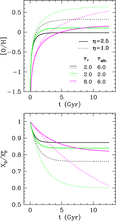
Figure 1.— Evolution of $[{\rm O}/{\rm H}]=\log_{10}Z_{\rm O}/Z_{{\rm O},\odot}$ (top) and the deuterium abundance (bottom, scaled to the primordial value) for a selection of one-zone models. Solid curves represent models with outflow mass loading factor $\eta=2.5$, while dotted curves adopt a lower $\eta=1.0$ that leads to super-solar oxygen abundance. Black curves show a typical SFE timescale ($\tau_{*}=2\,{\rm Gyr}$) and slowly declining SFH ($\tau_{\rm sfh}=6\,{\rm Gyr}$). Green curves show the same SFE but a rapidly falling SFH ($\tau_{\rm sfh}=2\,{\rm Gyr}$). Magenta curves show a model with inefficient star formation ($\tau_{*}=8\,{\rm Gyr}$) and slowly declining SFH ($\tau_{\rm sfh}=6\,{\rm Gyr}$).

Figure 1 plots the evolution of the oxygen and deuterium abundances for a variety of parameter choices. The solid black curves shows a case with an SFE timescale $\tau_{*}=2\,{\rm Gyr}$ typical of that found for molecular gas in star-forming galaxies (Leroy et al., 2008), a slowly declining star formation history with $\tau_{\rm sfh}=6\,{\rm Gyr}$, and a mass-loading parameter $\eta=2.5$ chosen to yield $Z_{\rm O,eq}$ near solar. With a depletion timescale of $0.65\,{\rm Gyr}$ (eq. 3), the oxygen abundance rises quickly to its equilibrium value, and deuterium declines to the corresponding equilibrium within $2\,{\rm Gyr}$. The solid green curves have $\tau_{\rm sfh}=2\,{\rm Gyr}$, which raises $Z_{\rm O,eq}$ because of the more rapidly declining gas supply. The equilibrium deuterium abundance is correspondingly lower. Magenta solid curves show a model with much lower star formation efficiency, $\tau_{*}=8\,{\rm Gyr}$. Here the approach to equilibrium is much slower, though both oxygen and deuterium are nearly constant after $t=10\,{\rm Gyr}$.

Dotted curves show the same cases but with a lower mass-loading factor $\eta=1.0$. Here the equilibrium oxygen abundances are higher because more of the metals produced by stars are retained, and the equilibrium deuterium abundances are lower because a larger fraction of the ISM consists of stellar ejecta. The lower outflow rate also lengthens the gas depletion time, and for $\tau_{*}=8\,{\rm Gyr}$ the abundances have not yet reached their equilibrium values by $t=12.5\,{\rm Gyr}$.

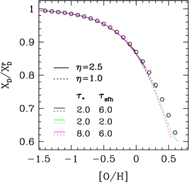
Figure 2.— Deuterium abundance, scaled to the primordial value, as a function of oxygen abundance $[{\rm O}/{\rm H}]$, for the models plotted in Fig. 1. Circles show the approximate formula $X_{\rm D}/X_{\rm D}^{\rm P}=1/(1+rZ_{\rm O}/m_{\rm O}^{\rm cc})$, where $r$ is the recycling fraction ($r=0.4$ in these models), $Z_{\rm O}$ is the ISM oxygen abundance by mass, and $m_{\rm O}^{\rm cc}$ is the IMF-averaged oxygen yield of CCSNe. The models represented by the green and magenta dotted curves have not reached equilibrium by $t=12.5\,{\rm Gyr}$; if they are extended further in time then they converge to the locus shown by the circles.

Figure 2 plots the evolution of these models in the plane of $X_{\rm D}/X_{\rm D}^{\rm P}$ vs. $[{\rm O}/{\rm H}]$. Remarkably, they are nearly superposed on a universal curve. Circles show the obvious generalization of equation (15),

$$X_{\rm D}={X_{\rm D}^{\rm P}\over 1+rZ_{\rm O}/m_{\rm O}^{\rm cc}}~{},$$ (16)

which simply assumes that the equilibrium relation also applies at earlier times. This formula describes the model results very well, though it slightly overpredicts $X_{\rm D}$ for super-solar $[{\rm O}/{\rm H}]$. I have tried other values of $r$ and $m_{\rm O}^{\rm cc}$ and find equally good agreement with equation (16).

Why does a formula derived for equilibrium abundances hold so well for systems that have not yet reached equilibrium? The mathematical answer is not obvious, but the ansatz of equation (16) is closely connected to the approximate argument given in the introduction. Suppose that the ISM consisted of a mix of primordial gas, with zero oxygen abundance, and gas that had been through stars precisely once, with oxygen abundance $m_{\rm O}^{\rm cc}/r$. The overall ISM oxygen abundance in this case would be $Z_{\rm O}=f_{\rm rec}m_{\rm O}^{\rm cc}/r=(1-f_{\rm prim})m_{\rm O}^{\rm cc}/r$, where $f_{\rm rec}$ and $f_{\rm prim}=1-f_{\rm rec}$ are the mass fractions of recycled and primordial material, respectively. The deuterium abundance is $X_{\rm D}^{\rm P}f_{\rm prim}$, and substituting for $f_{\rm prim}$ gives

$$X_{\rm D}\approx X_{\rm D}^{\rm P}(1-rZ_{\rm O}/m_{\rm O}^{\rm cc})~{},$$ (17)

which is equal to equation (16) at first order in $rZ_{\rm O}/m_{\rm O}^{\rm cc}$. Equation (17) is approximate because some gas in the recycled component has been through stars more than once, making the oxygen abundance in this component higher than $m_{\rm O}^{\rm cc}/r$, and it is somewhat less accurate than equation (16) at super-solar $[{\rm O}/{\rm H}]$. Nonetheless, the accuracy of equation (16) appears to be rooted in fairly basic accounting, and it becomes exact in the limit of equilibrium.

2.4. Metal-Enriched Winds

Equation (1) implicitly assumes that the gas ejected in winds has the current ISM abundance $Z_{\rm O}(t)$. If winds are driven by energy or momentum input from supernovae and massive stars, then it is possible that the metallicity of ejected material is higher than that of the ambient ISM, In the extreme limit, CCSN ejecta could escape from the galaxy without entraining ISM gas at all. The relation between ISM oxygen and deuterium abundances can set constraints on the degree of metal-enhancement in winds.

If the metallicity (specifically, the oxygen abundance) of ejected material is higher than that of ambient ISM gas by a factor

$$\xi_{\rm enh}={Z_{\rm wind}\over Z_{\rm ism}}~{},$$ (18)

then the third term on the r.h.s. of equation (1) is multiplied by $\xi_{\rm enh}$ while other terms are unchanged. The solution for oxygen evolution is the same as before except that $\eta$ is replaced by $\eta\xi_{\rm enh}$, the effective mass-loading factor for oxygen ejection, in both the equilibrium abundance (eq. 10) and the depletion timescale (eq. 3). Thus, for $\xi_{\rm enh}>1$ and a given $\eta$, oxygen evolves to a lower equilibrium abundance and reaches that equilibrium more quickly.

Deuterium evolution depends on the overall mass outflow rate, independent of $\xi_{\rm enh}$, so equation (13) and the first equality of equation (14) are unchanged. However, metal-enhanced winds alter the relation between the equilibrium deuterium and oxygen abundances to

$$X_{\rm D,eq}={X_{\rm D}^{\rm P}\over 1+\beta rZ_{\rm O,eq}^{\prime}/m_{\rm O}^{\rm cc}}$$ (19)

where $Z_{\rm O,eq}^{\prime}$ represents the equilibrium oxygen abundance in the metal-enhanced case and

$$\beta={1+\eta\xi_{\rm enh}-r-\tau_{*}/\tau_{\rm sfh}\over 1+\eta-r-\tau_{*}/\tau_{\rm sfh}}~{}.$$ (20)

For $\xi_{\rm enh}>1$, the deuterium abundance at a given oxygen abundance is lower. Physically, this lower $X_{\rm D,eq}$ arises because the mass loading factor $\eta$ required to produce the specified oxygen abundance is lower, and lower outflow implies correspondingly lower accretion at fixed SFR. Reduced accretion in turn implies that a larger fraction of the ISM consists of recycled stellar material, depleted in deuterium.

Figure 3 illustrates the magnitude of this effect, where I have adopted $\tau_{*}=2.0\,{\rm Gyr}$ and $\tau_{\rm sfh}=6.0\,{\rm Gyr}$. For each value of $\xi_{\rm enh}$, the value of $\eta$ is chosen to yield a solar equilibrium abundance (solid curve) or $[{\rm O}/{\rm H}]_{\rm eq}=-0.2$ (dotted curve) or +0.1 (dashed curve). The equilibrium deuterium abundance decreases with increasing $\xi_{\rm enh}$, as implied by equation (19). For example, achieving solar oxygen abundance in the standard case of $Z_{\rm wind}=Z_{\rm ISM}$ requires $\eta=2.4$, with an equilibrium $X_{\rm D,eq}/X_{\rm D}^{\rm P}=0.87$. However, with a metal-enhancement factor $\xi_{\rm enh}=2$, the required value of $\eta$ is 1.2, and the implied $X_{\rm D,eq}/X_{\rm D}^{\rm P}=0.79$. Unfortunately, dust depletion uncertainties make precise determinations of $({\rm D}/{\rm H})_{\rm ISM}$ challenging, but this value is probably at the lower limit of the acceptable range from Linsky et al. (2006). Metal enhancement with $\xi_{\rm enh}\geq 3$, implying $X_{\rm D,eq}/X_{\rm D}^{\rm P}\leq 0.73$, would be difficult to reconcile with the observed deuterium abundance. There is no obvious physical mechanism for producing metal-depleted outflows ($\xi_{\rm enh}<1$), but if they occurred they would lead to higher $X_{\rm D}$ at a given $[{\rm O}/{\rm H}]$.

Figure 3.— Ratio of equilibrium deuterium abundance to the primordial abundance as a function of the enhancement factor $\xi_{\rm enh}=Z_{\rm wind}/Z_{\rm ISM}$, the ratio of wind metallicity to ISM metallicity. Solid, dotted, and dashed curves show cases in which the equilibrium oxygen abundance is solar, $[{\rm O}/{\rm H}]=-0.2$, and $[{\rm O}/{\rm H}]=+0.1$, respectively. All cases assume $\tau_{*}/\tau_{\rm sfh}=1/3$.

2.5. Numerical Examples

The analytic solutions here apply to a restricted class of models, so to investigate other cases I have written a simple numerical code that integrates the governing differential equations (1) and (11). Figure 4 compares three different models to a fiducial analytic model with constant SFE timescale $\tau_{*}=2\,{\rm Gyr}$, an exponential star formation history with $\tau_{\rm sfh}=6\,{\rm Gyr}$, and $\eta=2.5$. Observed star formation laws (Schmidt, 1959; Kennicutt, 1998) show a non-linear relation between SFR surface density and total gas surface density, approximately $\Sigma_{\rm SFR}\propto\Sigma_{g}^{1.5}$. If we think of a one-zone chemical evolution model as representing an annulus of the Galactic disk, we might therefore expect the SFE timescale to grow as the gas surface density decreases, with $\tau_{*}\propto M_{g}^{-0.5}$. Red curves show a numerical model with this SFE scaling and the same exponential star formation history. The predicted evolutionary track of $X_{\rm D}/X_{\rm D}^{\rm P}$ vs. $[{\rm O}/{\rm H}]$ is indistinguishable from that of the constant $\tau_{*}$ model and in excellent agreement with equation (16).

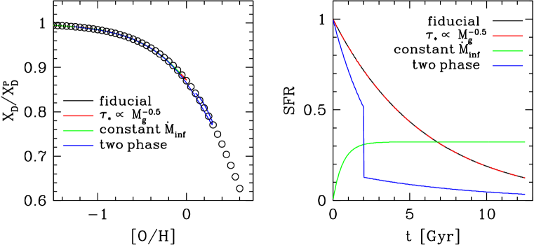
Figure 4.— Evolutionary tracks of $X_{\rm D}/X_{\rm D}^{\rm P}$ vs. $[{\rm O}/{\rm H}]$ (left) for models with star formation histories shown in the right panel. Black curves show our fiducial exponential model with constant $\tau_{*}$, red curves a model with the same star formation history and “Schmidt Law” $\tau_{*}$ scaling, green curves a model with constant mass infall rate, and blue curves a model in which star formation parameters and $\eta$ change suddenly at $t=2\,{\rm Gyr}$ (see text). Evolutionary tracks are nearly indistinguishable and agree well with equation (16) shown by open circles, but one can see that the two phase model loops back to lower $[{\rm O}/{\rm H}]$ and higher $X_{\rm D}/X_{\rm D}^{\rm P}$ after $\eta$ changes from 1 to 2.

Green curves show a model with constant $\tau_{*}=2\,{\rm Gyr}$ and a constant mass infall rate of $1M_{\odot}\,{\rm yr}^{-1}$, again with $\eta=2.5$. With zero initial gas mass, the star formation rate of this model rises linearly at early times and asymptotes to an equilibrium value of $\dot{M}_{*}=\dot{M}_{\rm inf}/(1+\eta-r)$. Despite the very different star formation history (as shown in the right panel), the track of this model in the $X_{\rm D}$-$[{\rm O}/{\rm H}]$ plane is indistinguishable from those of the exponential models. Blue curves show a model with a sharp transition of parameters at $t=2\,{\rm Gyr}$, from efficient early star formation with low outflow mass loading ($\tau_{*}=1\,{\rm Gyr}$, $\tau_{\rm sfh}=3\,{\rm Gyr}$, $\eta=1$) to slower star formation and higher outflow efficiency ($\tau_{*}=4\,{\rm Gyr}$, $\tau_{\rm sfh}=8\,{\rm Gyr}$, $\eta=2$) at later times. Because of the low initial $\eta$, this model first evolves to super-solar $[{\rm O}/{\rm H}]$ and $X_{\rm D}/X_{\rm D}^{\rm P}\approx 0.78$. After the transition to higher $\eta$, it loops back to a new equilibrium at lower $[{\rm O}/{\rm H}]$ and higher $X_{\rm D}/X_{\rm D}^{\rm P}$, approximately but not exactly reversing its original evolutionary track.

Although these examples are not exhaustive, they suggest that the behavior of equation (16) applies to a wide range of models, provided that outflows eject gas at the ISM metallicity.

2.6. Supernova Yields and the IMF

The key parameters influencing the relation between oxygen abundance and deuterium abundance are the oxygen yield $m_{\rm O}^{\rm cc}$ and the recycling fraction $r$. For a Kroupa (2001) IMF truncated at $0.1M_{\odot}$ and $100M_{\odot}$, the solar metallicity supernova yields of Limongi & Chieffi (2006) yield $m_{\rm O}^{\rm cc}=0.017$ assuming that all stars above $8M_{\odot}$ explode as CCSNe (see Andrews et al. 2017 for details of the IMF-averaged yield calculation). However, the predicted oxygen production is a steeply increasing function of progenitor mass, and if the most massive stars collapse to form black holes instead of exploding then the IMF-averaged yield can be significantly reduced. The left panel of Figure 5 shows the predicted value of $X_{\rm D}/X_{\rm D}^{\rm P}$ at solar $[{\rm O}/{\rm H}]$, computed from equation (16), assuming that all stars with $M>M_{\rm SN,max}$ collapse to form black holes and release no oxygen. I have used the recycling fraction $r=0.4$, appropriate for a Kroupa (2001) IMF after 2 Gyr, and I have ignored the small impact of black hole formation on $r$ under the assumption that massive stars still return most of the mass they were born with. For a cutoff $M_{\rm SN,max}<37M_{\odot}$ the predicted $X_{\rm D}/X_{\rm D}^{\rm P}$ falls below 0.8, in tension with the Linsky et al. (2006) ISM estimates.

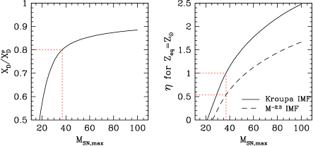
Figure 5.— (Left) Influence of the upper mass cutoff for supernovae on the predicted deuterium abundance at solar metallicity, computed for a Kroupa (2001) IMF with the oxygen yields of Limongi & Chieffi (2006). A value $M_{\rm SN,max}=37M_{\odot}$ yields $X_{\rm D}/X_{\rm D}^{\rm P}=0.8$, the $1\sigma$ lower bound on the ISM deuterium abundance from Linsky et al. (2006). (Right) The value of $\eta$ required to yield solar oxygen abundance at equilibrium, as a function of $M_{\rm SN,max}$. The solid curve shows results for a Kroupa (2001) IMF and the dashed curve for an $M^{-2.3}$ power-law IMF that extends down to $0.1M_{\odot}$. A $37M_{\odot}$ supernova cutoff corresponds to $\eta=1.0$ or 0.54 in these two cases. Changing the IMF at low masses (below the main sequence turnoff) does not influence the predicted $Y_{D}$ because it has canceling effects on $m_{\rm O}^{\rm cc}$ and $r$.

The right panel of Figure 5 shows the value of $\eta$ required to produce $Z_{\rm O,eq}=Z_{\rm O,\odot}$,

$$\eta={m_{\rm O}^{\rm cc}\over Z_{\rm O,\odot}}+r-1-\tau_{*}/\tau_{\rm sfh}~{},$$ (21)

assuming $r=0.4$ and $\tau_{*}/\tau_{\rm sfh}=1/3$ as in the fiducial model. As $m_{\rm O}^{\rm cc}$ decreases with decreasing $M_{\rm SN,max}$, the required value of $\eta$ also drops. However, values of $M_{\rm SN,max}$ that imply $\eta\lesssim 1$ also imply $X_{\rm D}/X_{\rm D}^{\rm P}\lesssim 0.8$, so one cannot eliminate the need for outflows by reducing the oxygen yield without running afoul of the deuterium constraint.

The Kroupa (2001) IMF scales as $M^{-2.3}$ for $M>0.5M_{\odot}$ and as $M^{-1.3}$ for $M=0.1-0.5M_{\odot}$. A pure $M^{-2.3}$ power law IMF has more low mass stars, increasing the total mass of the stellar population by a factor $\approx 1.3$ for the same number of high mass stars. (A Salpeter [1955] IMF has a slightly steeper, $M^{-2.35}$ slope.) The dashed curve in Figure 5 shows the value of $\eta$ implied by equation (21) after reducing both $m_{\rm O}^{\rm cc}$ and $r$ by this factor of 1.3. Adding low mass stars does not change the $X_{\rm D}/X_{\rm D}^{\rm P}$ results shown in the left panel because the changes to $m_{\rm O}^{\rm cc}$ and $r$ cancel in equation (16). A bottom-heavy IMF reduces the level of outflow required to achieve a solar ISM oxygen abundance, but reducing $\eta$ to zero is still not possible without an observationally unacceptable level of deuterium depletion. A bottom-heavy IMF of this sort also conflicts with the observed stellar populations of the local disk (Kroupa, 2001; Chabrier, 2003) and with the dynamical mass-to-light ratios of spiral galaxies (Bell & de Jong, 2001).

3. Implications

The results in §2 agree with those of more sophisticated models of galactic chemical evolution (GCE), which generally yield ISM deuterium abundances only moderately below the primordial abundance when they are tuned to reproduce observations of the solar neighborhood (e.g., Tosi et al. 1998; Romano et al. 2006; Steigman et al. 2007; Lagarde et al. 2012). The simplicity of the arguments leading to equations (15) and (16) implies that this behavior should be robust to details of the GCE model, and it shows that the most important assumptions are likely those that affect the oxygen yield $m_{\rm O}^{\rm cc}$ and the recycling fraction $r$. The numerical examples illustrated in Figure 4 provide further support for the robustness of this prediction. A mixture of gas from zones that individually obey equation (16) will also follow equation (16) if $rZ_{\rm O}/m_{\rm O}^{\rm cc}\ll 1$ (allowing a linear Taylor expansion) and the level of deuterium depletion is therefore small in each zone. However, a mixture of high-metallicity, heavily depleted gas with low-metallicity, low depletion gas would initially lie above this locus (high deuterium abundance relative to $[{\rm O}/{\rm H}]$), then return to it as further star formation drove the system toward equilibrium. It is thus likely but not guaranteed that equation (16) will remain accurate in more sophisticated GCE models that incorporate ingredients such as radial gas flows and fountain recycling.

The close links predicted between oxygen and deuterium abundances strengthen arguments (Draine, 2006; Linsky et al., 2006; Steigman et al., 2007) that sightline-to-sightline variations of $({\rm D}/{\rm H})$ absorption are caused by depletion of deuterium onto dust, as originally proposed by Jura (1982). This explanation requires a large fraction of the available sites on polycyclic aromatic hydrocarbon (PAH) molecules to be occupied by deuterium rather than hydrogen, but the energy differences associated with the heavier deuterium nucleus permit this preferential outcome in the cool ISM, and reaction rates appear high enough to achieve it (Draine, 2006). Producing factor-of-two variations in $({\rm D}/{\rm H})$ by differential astration, on the other hand, would induce enormous variations in $({\rm O}/{\rm H})$, since it would require a much larger fraction of the ISM on low $({\rm D}/{\rm H})$ sightlines to be comprised of stellar ejecta. The alternative of setting the mean ISM $({\rm D}/{\rm H})$ to $\sim 1-1.5\times 10^{-5}$ and producing high $({\rm D}/{\rm H})$ by localized infall of primordial gas would require a major revision of oxygen yields to avoid overproducing oxygen. With our adopted $m_{\rm O}^{\rm cc}=0.015$, reaching $({\rm D}/{\rm H})=1.0\times 10^{-5}$ implies $[{\rm O}/{\rm H}]=+1.0$, and $({\rm D}/{\rm H})=1.5\times 10^{-5}$ implies $[{\rm O}/{\rm H}]=+0.7$.

Many studies have used $({\rm D}/{\rm H})$ in low metallicity, extragalactic Lyman-$\alpha$ absorption systems to estimate the primordial $({\rm D}/{\rm H})$ ratio and thereby constrain the mean baryon density (e.g., Cooke et al. 2014 and references therein). The baryon density inferred from observations of the cosmic microwave background (Hinshaw et al., 2013; Planck Collaboration et al., 2016) agrees well with that inferred from $({\rm D}/{\rm H})$ observations, an important cosmological consistency test that constrains non-standard BBN models (Cyburt et al., 2016; Nollett & Steigman, 2015). Equation (16) implies that evolutionary corrections to $({\rm D}/{\rm H})$ should be small in systems with sub-solar oxygen abundance, and there is no need to seek out ultra-low metallicity systems to eliminate these corrections. The primary reason to concentrate on low metallicity sightlines for cosmological $({\rm D}/{\rm H})$ studies is to reduce uncertainties associated with dust depletion. Dvorkin et al. (2016), using more sophisticated chemical evolution models based on cosmologically motivated infall rates, reach similar conclusions about the small impact of deuterium depletion in damped Lyman-$\alpha$ systems and the tight expected correlation between oxygen and deuterium abundance.

Like deuterium, ${}^{3}{\rm He}$ is produced in BBN at fairly high abundance, $(^{3}{\rm He}/{\rm H})_{\rm P}\approx 10^{-5}$ (Cyburt et al., 2016). In contrast to deuterium, ${}^{3}{\rm He}$ can be produced in stars as well as destroyed (Iben, 1967; Truran & Cameron, 1971; Rood et al., 1976; Dearborn et al., 1996), so even the sign of evolutionary corrections is not obvious without detailed modeling. The arguments presented here suggest that the magnitude of ${}^{3}{\rm He}$ destruction should be small because most ISM gas has not been processed by stars at all. Observations indicate an ISM ${}^{3}{\rm He}$ abundance that is not far from the BBN value (Gloeckler & Geiss, 1996; Bania et al., 2002). In concert with minimal destruction, this small amount of evolution implies that production of ${}^{3}{\rm He}$ by stellar nucleosynthesis must be small. As discussed in detail by Lagarde et al. (2012), this result is a challenge to conventional stellar evolution models but is well explained by models that incorporate thermohaline mixing.

The robustness of the $({\rm D}/{\rm H})$ prediction to detailed assumptions implies that deuterium observations provide only limited constraints on standard GCE models; most models that produce solar $[{\rm O}/{\rm H}]$ should predict $({\rm D}/{\rm H})$ that matches current observations within their uncertainties. However, if dust depletion uncertainties can be controlled, then precise $({\rm D}/{\rm H})$ measurements could provide a useful test of yield and recycling values, especially if deuterium can be mapped over a wide enough range of metallicity to demonstrate the behavior predicted by equation (16). As shown in Figure 5, the constraint $X_{\rm D}/X_{\rm D}^{\rm P}\geq 0.8$ is already enough to challenge otherwise plausible scenarios in which most stars above $30M_{\odot}$ collapse to black holes instead of releasing oxygen in supernovae (see discussions by, e.g., Pejcha & Thompson 2015; Sukhbold et al. 2016).

As discussed in §2.4, the prediction of equations (15) and (16) is violated in models where outflows preferentially drive out CCSN ejecta while retaining the AGB ejecta returned over longer timescales. This scenario allows more return of deuterium-depleted hydrogen for a given amount of oxygen, so it predicts lower $({\rm D}/{\rm H})$ as a function of $[{\rm O}/{\rm H}]$. The agreement of observed abundances with simple predictions disfavors metal-enhanced winds with $\xi_{\rm enh}\gtrsim 2$. Models in which radiation pressure ejects galactic dust with minimal gas entrainment (e.g., Aguirre et al. 2001) could also violate $({\rm D}/{\rm H})$ constraints, though here one must take account of the potentially high fraction of deuterium residing in ejected dust.

The analytic models presented here adopt the instantaneous recycling approximation, and models in which the SFR or outflow efficiency change rapidly compared to the $\sim 1\,{\rm Gyr}$ timescale of AGB recycling could lead to significantly different $({\rm D}/{\rm H})$ predictions. For example, even with constant $\eta$ and $\xi_{\rm enh}=1$, a 100 Myr starburst could eject most of the oxygen produced by its supernovae while allowing deuterium-depleted gas to return from AGB envelopes after the burst has ended. Consistent with this picture, the models of Dvorkin et al. (2016) that incorporate extreme early star formation predict lower $({\rm D}/{\rm H})$ than their smoother models. We leave numerical investigation of bursty models with continuous AGB recycling to future work.

Theoretical models of galaxy formation require feedback from star formation to reproduce observed galaxy properties, and vigorously star-forming galaxies at low and high redshift show abundant evidence of outflowing gas. However, there is little direct observational evidence of winds in “normal” star-forming galaxies like the Milky Way at $z=0$. chemical evolution models suggest that outflows with substantial mass-loading factors are required to produce near-solar metallicity ISM abundances, as illustrated in Figure 5. The high observed deuterium abundance in the local ISM closes off two of the most obvious loopholes in this argument: low IMF-averaged oxygen yields and outflows that eject a large fraction of supernova metals with little entrainment of the ambient ISM.

The robust link between oxygen and deuterium abundances should also inform the lectures that we give to our introductory astronomy astronomy students. In the H₂O molecules that make up 2/3 of our body mass, every oxygen atom was born in the nuclear furnace of a stellar interior. But the hydrogen atoms? 90% of them come straight from the big bang.

References

- Aguirre et al. (2001) Aguirre, A., Hernquist, L., Katz, N., Gardner, J., & Weinberg, D. 2001, ApJ, 556, L11
- Andrews et al. (2017) Andrews, B. H., Weinberg, D. H., Schönrich, R., & Johnson, J. A. 2017, ApJ, 835, 224
- Balser et al. (2011) Balser, D. S., Rood, R. T., Bania, T. M., & Anderson, L. D. 2011, ApJ, 738, 27
- Bania et al. (2002) Bania, T. M., Rood, R. T., & Balser, D. S. 2002, Nature, 415, 54
- Bell & de Jong (2001) Bell, E. F., & de Jong, R. S. 2001, ApJ, 550, 212
- Bensby et al. (2014) Bensby, T., Feltzing, S., & Oey, M. S. 2014, A&A, 562, A71
- Bodenheimer (1966) Bodenheimer, P. 1966, ApJ, 144, 103
- Cavichia et al. (2014) Cavichia, O., Mollá, M., Costa, R. D. D., & Maciel, W. J. 2014, MNRAS, 437, 3688
- Chabrier (2003) Chabrier, G. 2003, ApJ, 586, L133
- Chieffi & Limongi (2004) Chieffi, A., & Limongi, M. 2004, ApJ, 608, 405
- Coc et al. (2015) Coc, A., Petitjean, P., Uzan, J.-P., et al. 2015, Phys. Rev. D, 92, 123526
- Cooke et al. (2014) Cooke, R. J., Pettini, M., Jorgenson, R. A., Murphy, M. T., & Steidel, C. C. 2014, ApJ, 781, 31
- Cyburt et al. (2016) Cyburt, R. H., Fields, B. D., Olive, K. A., & Yeh, T.-H. 2016, Reviews of Modern Physics, 88, 015004
- Dearborn et al. (1996) Dearborn, D. S. P., Steigman, G., & Tosi, M. 1996, ApJ, 465, 887
- Draine (2006) Draine, B. T. 2006, in Astronomical Society of the Pacific Conference Series, Vol. 348, Astrophysics in the Far Ultraviolet: Five Years of Discovery with FUSE, ed. G. Sonneborn, H. W. Moos, & B.-G. Andersson, 58
- Dvorkin et al. (2016) Dvorkin, I., Vangioni, E., Silk, J., Petitjean, P., & Olive, K. A. 2016, MNRAS, 458, L104
- Edvardsson et al. (1993) Edvardsson, B., Andersen, J., Gustafsson, B., et al. 1993, A&A, 275, 101
- Feuillet et al. (2016) Feuillet, D. K., Bovy, J., Holtzman, J., et al. 2016, ApJ, 817, 40
- Finlator & Davé (2008) Finlator, K., & Davé, R. 2008, MNRAS, 385, 2181
- Gloeckler & Geiss (1996) Gloeckler, G., & Geiss, J. 1996, Nature, 381, 210
- Hinshaw et al. (2013) Hinshaw, G., Larson, D., Komatsu, E., et al. 2013, ApJS, 208, 19
- Iben (1967) Iben, Jr., I. 1967, ApJ, 147, 624
- Jura (1982) Jura, M. 1982, in NASA Conference Publication, Vol. 2238, NASA Conference Publication, ed. Y. Kondo, 54–60
- Kennicutt (1998) Kennicutt, Jr., R. C. 1998, ApJ, 498, 541
- Kroupa (2001) Kroupa, P. 2001, MNRAS, 322, 231
- Lagarde et al. (2012) Lagarde, N., Romano, D., Charbonnel, C., et al. 2012, A&A, 542, A62
- Larson (1972) Larson, R. B. 1972, Nature, 236, 21
- Leroy et al. (2008) Leroy, A. K., Walter, F., Brinks, E., et al. 2008, AJ, 136, 2782
- Limongi & Chieffi (2006) Limongi, M., & Chieffi, A. 2006, ApJ, 647, 483
- Linsky et al. (2006) Linsky, J. L., Draine, B. T., Moos, H. W., et al. 2006, ApJ, 647, 1106
- Lodders (2003) Lodders, K. 2003, ApJ, 591, 1220
- Marconi et al. (1994) Marconi, G., Matteucci, F., & Tosi, M. 1994, MNRAS, 270, 35
- Matteucci & Greggio (1986) Matteucci, F., & Greggio, L. 1986, A&A, 154, 279
- Mazzitelli & Moretti (1980) Mazzitelli, I., & Moretti, M. 1980, ApJ, 235, 955
- Mollá & Díaz (2005) Mollá, M., & Díaz, A. I. 2005, MNRAS, 358, 521
- Nollett & Steigman (2014) Nollett, K. M., & Steigman, G. 2014, Phys. Rev. D, 89, 083508
- Nollett & Steigman (2015) —. 2015, Phys. Rev. D, 91, 083505
- Peeples & Shankar (2011) Peeples, M. S., & Shankar, F. 2011, MNRAS, 417, 2962
- Pejcha & Thompson (2015) Pejcha, O., & Thompson, T. A. 2015, ApJ, 801, 90
- Pilyugin (1993) Pilyugin, L. S. 1993, A&A, 277, 42
- Planck Collaboration et al. (2016) Planck Collaboration, Ade, P. A. R., Aghanim, N., et al. 2016, A&A, 594, A13
- Recchi et al. (2008) Recchi, S., Spitoni, E., Matteucci, F., & Lanfranchi, G. A. 2008, A&A, 489, 555
- Romano et al. (2006) Romano, D., Tosi, M., Chiappini, C., & Matteucci, F. 2006, MNRAS, 369, 295
- Rood et al. (1976) Rood, R. T., Steigman, G., & Tinsley, B. M. 1976, ApJ, 207, L57
- Rudolph et al. (2006) Rudolph, A. L., Fich, M., Bell, G. R., et al. 2006, ApJS, 162, 346
- Salpeter (1955) Salpeter, E. E. 1955, ApJ, 121, 161
- Schmidt (1959) Schmidt, M. 1959, ApJ, 129, 243
- Spitoni (2015) Spitoni, E. 2015, MNRAS, 451, 1090
- Spitoni & Matteucci (2011) Spitoni, E., & Matteucci, F. 2011, A&A, 531, A72
- Spitoni et al. (2017) Spitoni, E., Vincenzo, F., & Matteucci, F. 2017, A&A, 599, A6
- Steigman et al. (2007) Steigman, G., Romano, D., & Tosi, M. 2007, MNRAS, 378, 576
- Sukhbold et al. (2016) Sukhbold, T., Ertl, T., Woosley, S. E., Brown, J. M., & Janka, H.-T. 2016, ApJ, 821, 38
- Tosi et al. (1998) Tosi, M., Steigman, G., Matteucci, F., & Chiappini, C. 1998, ApJ, 498, 226
- Truran & Cameron (1971) Truran, J. W., & Cameron, A. G. W. 1971, Ap&SS, 14, 179
- van de Voort et al. (2017) van de Voort, F., Quataert, E., Faucher-Giguère, C.-A., et al. 2017, ArXiv e-prints, arXiv:1704.08254
- Weinberg et al. (2017) Weinberg, D. H., Andrews, B. H., & Freudenburg, J. 2017, ApJ, 837, 183
- Zahid et al. (2012) Zahid, H. J., Dima, G. I., Kewley, L. J., Erb, D. K., & Davé, R. 2012, ApJ, 757, 54