The Hunt for Planet Nine: Atmosphere, Spectra, Evolution, and Detectability

Abstract

We investigate the physical characteristics of the Solar System’s proposed Planet Nine using modeling tools with a heritage in studying Uranus and Neptune. For a range of plausible masses and interior structures, we find upper limits on the intrinsic $T_{\rm eff}$, from $\sim$35-50 K for masses of 5-20 $M_{\oplus}$, and we also explore lower $T_{\rm eff}$ values. Possible planetary radii could readily span from 2.7 to 6 $R_{\oplus}$ depending on the mass fraction of any H/He envelope. Given its cold atmospheric temperatures, the planet encounters significant methane condensation, which dramatically alters the atmosphere away from simple Neptune-like expectations. We find the atmosphere is strongly depleted in molecular absorption at visible wavelengths, suggesting a Rayleigh scattering atmosphere with a high geometric albedo approaching 0.75. We highlight two diagnostics for the atmosphere’s temperature structure, the first being the value of the methane mixing ratio above the methane cloud. The second is the wavelength at which cloud scattering can be seen, which yields the cloud-top pressure. Surface reflection may be seen if the atmosphere is thin. Due to collision-induced opacity of H₂ in the infrared, the planet would be extremely blue (instead of red) in the shortest wavelength WISE colors if methane is depleted, and would, in some cases, exist on the verge of detectability by WISE. For a range of models, thermal fluxes from $\sim 3-5$ $\mu$m are $\sim$ 20 orders of magnitude larger than blackbody expectations. We report a search of the AllWISE Source Catalog for Planet Nine, but find no detection.

1. Introduction

Recently, Batygin & Brown (2016) have found that the orbits of long period Kuiper Belt Objects cluster in their arguments of perihelion and also in physical space in the solar system. They suggest that dynamical perturbations arising from a relatively small giant planet of perhaps 10 $M_{\oplus}$, on an eccentric orbit with a semi-major axis distance of perhaps $a\sim$ 700 AU, can explain this clustering.

The formation, evolution, and detectability of this possible “Planet Nine” has been the target of intense study (de la Fuente Marcos & de la Fuente Marcos, 2016; Malhotra et al., 2016; Li & Adams, 2016; Linder & Mordasini, 2016; Cowan et al., 2016; Fienga et al., 2016; Ginzburg et al., 2016; Brown & Batygin, 2016; Kenyon & Bromley, 2016; Bromley & Kenyon, 2016; Mustill et al., 2016; Holman & Payne, 2016). To date, studies that have included discussion of the atmosphere, emission, or cooling history of the planet have focused on Planet Nine as a blackbody. This is certainly a valid starting point, especially since nothing is yet known about this possible object. Yet a straightforward, but more detailed look at the planet yields a better understanding of the planet’s atmosphere, evolution, and spectra that cannot come out of simple analysis. For instance, the spectra of the solar system’s giant planets differ strongly from blackbodies.

Planet Nine, if it exists, may have a mass between that of Earth and Uranus. Exoplanets in this mass range are extremely common (Borucki et al., 2011). Should Planet Nine be detected, the characterization of the planet would either confirm or refute studies such as the one we present here, and could serve as a proxy for the physical and atmospheric properties of the as-yet largely unstudied worlds that are among the most common outcomes of the planetary formation process.

In this Letter we first investigate the cooling history of the Planet Nine, over a wide range of possible masses from 5–50 $M_{\oplus}$. Here we assume a planet that has at least some H/He atmosphere, in analogy with Uranus and Neptune as well as the thousands of sub-Neptune exoplanets that suggest a non-negligible H/He envelope (Lopez & Fortney, 2014). We draw connections between the cooling history of Planet Nine and our incomplete understanding of the thermal evolution of Uranus and Neptune. With fluxes from the planet’s interior and from the Sun then reasonably well-bounded, we can begin to estimate the atmospheric temperature structure. We assess the condensation of methane, atmospheric opacity sources, and the spectrum of the planet from optical to thermal infrared wavelengths, focusing on novel and at times counter-intuitive behavior at very low temperature ($\sim 30-40$ K). Finally, we apply these findings to a revised assessment of the detectability of Planet Nine and report on a new search of the WISE catalog.

2. Thermal Evolution

2.1. Method

In order to estimate the possible radius and intrinsic luminosity of Planet Nine we have run Neptune-like thermal evolution models, where we varied several structure parameters around those appropriate for Neptune. These models are somewhat similar to those of Linder & Mordasini (2016), although we make different choices about particular compositions to investigate. Here we assume planet masses between 5 and 50 $M_{\oplus}$ ($M_{\rm Nep}=17.15$ $M_{\oplus}$) and two compositionally different layers consisting of a H/He envelope atop a core that is either ice-rich (2$\,:\,$1 ice$\,:\,$rock) or ice-poor (1$\,:\,$4 ice$\,:\,$rock). We varied the core mass fraction within 0.1–0.3 for the most massive models, representing a sub-Saturn mass gas giant, 0.30–0.84 for a 15$M_{\oplus}$ series of models, and 0.6–0.9 for the least massive models of 5–8 $M_{\oplus}$, representing a sub-Neptune. For reference, constraints from Neptune suggest $\sim$ 0.76–0.90 ice/rock by mass (Helled et al., 2011; Nettelmann et al., 2013), and detailed modeling suggests a ice-enriched H/He envelope atop very ice/rock rich deep interior (Hubbard et al., 1995; Helled et al., 2011; Nettelmann et al., 2013). Like Nettelmann et al. (2013) we represent the warm fluid ices in the interior by the water equation of state (EOS) H₂O-REOS.1, H/He the updated H/He-REOS.3 tables of Becker et al. (2014), and for the rock EOS Hubbard & Marley (1989).

We followed the thermal evolution of Planet Nine at 1000 AU, corresponding to a zero-albedo equilibrium temperature of 9 K. We explored a range of incident fluxes but found that is yielded little impact on the thermal evolution. For the upper boundary condition, the radiative atmosphere, we applied an analytic description (Guillot et al., 1995) of to the non-gray Graboske et al. (1975) model atmosphere grid, which relates the 1-bar temperature (and hence the specific entropy of the interior adiabat) and surface gravity to the $T_{\rm eff}$. For the constant of proportionality between the 1-bar temperature and the $T_{\rm eff}$ we use $K=1.50$ based on Neptune. We assume a hot start initial condition (e.g. Marley et al., 2007) and then adiabatic cooling thereafter. At all points in the evolutionary history we track the evolution of the intrinsic luminosity and radius. See Nettelmann et al. (2013) for further modeling details.

2.2. Results

Our modelling results for Planet Nine are summarized in Table 1. We recover the strong influence of the assumed H/He mass fraction on the resulting radius, as it is well known from mass-radius relations for warm exoplanets (e.g., Fortney et al., 2007; Lopez & Fortney, 2014). In particular, the radius of Planet Nine may reach from 2.7 to 4.4 $R_{\oplus}$ if its mass is within 5–8 $M_{\oplus}$, or from 3.6 to 6.7 $R_{\oplus}$ if 15–20 $M_{\oplus}$ (Neptune: 3.9 $R_{\oplus}$), and further to 6.4–8.3 $R_{\oplus}$ if 35–50 $M_{\oplus}$. Intrinsic temperatures range from the Uranian upper limit of $T_{\rm int}\sim 40K$ if $M\leq 12$$M_{\oplus}$to sub-Saturn like values of $T_{\rm int}\sim 60$ K for $M=50$ $M_{\oplus}$. As expected, we find $T_{\rm int}$ to rise with planet mass, but, surprisingly, to decrease with H/He content. The latter behavior results from the larger energy that can be radiated away from a larger surface area, and from the low internal temperatures along the H/He adiabats at $\sim 1$ Mbar pressures.

On the whole, we find excellent agreement with the findings of Linder & Mordasini (2016). We agree that the planet’s luminosity is likely strongly dominated by intrinsic flux, rather than re-radiated solar energy. Specifically, they suggest a $T_{\rm eff}$ of 47 K for a 10 $M_{\oplus}$ planet model with a 1:1 ice:rock core and 1.4 $M_{\oplus}$ envelope, which suggests an agreement within a few Kelvin for our cooling models, based on our Table 1.

These results should be taken with significant caution. While adiabatic cooling models can reproduce the current intrinsic flux from Neptune, they significantly overestimate the flux from within Uranus, which has been an outstanding problem for decades (Hubbard et al., 1995; Fortney & Nettelmann, 2010). Therefore these $T_{\rm int}$ and $T_{\rm eff}$ values should be taken as upper limits. Below, when modeling the atmosphere we examine $T_{\rm int}$ values down to 20 K, lower than that predicted by our evolutionary calculations.

Planet	Core	H/He Env.	I:R	Planet	$T_{\rm eff}$	$T_{\rm 1bar}$	$T_{\rm int}$
Mass ($M_{\oplus}$)	Mass	Mass	Ratio	Radius ($R_{\oplus}$)	(K)	(K)	(K)
5	3	2	2:1	4.12	36.7	51.6	36.5
5	4.5	0.5	2:1	2.94	42.2	54.6	41.7
5	4.5	0.5	1:4	2.71	38.9	48.1	36.8
8	5	3	2:1	4.44	39.5	55.4	39.2
8	7	1	2:1	3.44	46.2	59.7	47.2
8	7	1	1:4	3.17	42.6	52.5	40.8
10	5	5	2:1	5.09	40.3	55.3	40.1
10	9	1	2:1	3.46	48.3	60.9	47.8
10	9	1	1:4	3.16	45.1	54.3	42.2
12	5	7	2:1	5.57	41.4	57.1	41.2
12	10	2	2:1	3.93	46.1	58.2	45.7
12	10	2	1:4	3.64	44.6	52.3	42.8
15	5	10	2:1	6.16	43.2	62.4	42.8
15	13	2	2:1	3.92	48.7	60.0	48.2
15	13	2	1:4	3.63	46.8	55.6	45.0
20	5	15	2:1	6.74	46.2	63.1	46.1
20	15	5	2:1	4.72	50.6	63.7	50.2
20	15	5	1:4	4.48	50.2	62.0	49.1
35	5	30	2:1	7.76	53.5	73.5	53.5
35	15	20	2:1	6.60	57.5	76.2	57.3
35	15	20	1:4	6.44	57.1	74.8	56.6
50	5	45	2:1	8.33	59.5	81.0	59.3
50	15	35	2:1	7.50	63.3	84.3	63.2
50	15	35	1:4	7.37	62.8	83.0	62.5

Note. — Results of thermal evolution models for planets at 4.5 Gyr.

3. Atmosphere and Spectra

With these upper limits on the flux from the planet’s interior, we can begin to assess the state of the planet’s atmosphere. To model the pressure–temperature (P–T) profile, chemical abundances, and spectrum of the planet we use a model atmosphere code with a long heritage, including Titan (McKay et al., 1989), Uranus (Marley & McKay, 1999), and also a wide array of brown dwarfs (Marley et al., 1996; Morley et al., 2014) and exoplanets (Fortney et al., 2008; Marley et al., 2012). The predicted chemical equilibrium abundances follow the methods of Visscher et al. (2010).

For the initial exploration of this paper we choose five values for the intrinsic flux, $T_{\rm int}$, of 20, 30, 40, 50, and 60 K. There are also some additional modeling choices and constraints, which have caveats. At these cold temperatures, methane (CH₄) condenses out and leaves the gas phase. In our normal modeling efforts of relatively warmer objects, for instance water condensation into clouds in cool brown dwarfs, we calculate the vapor pressure of water above any cloud, to self-consistently determine the gaseous water mixing ratio at any P–T point (e.g., Morley et al., 2014). Given the large uncertainties for this possible planet, here we take a simpler path. We choose an opacity grid calculated at solar metallicity, but deplete these opacities by various factors to simulate the loss of methane. We also use an opacity database that is only complete above 75 K for most molecules (and 100 K for H₂) (Freedman et al., 2014), such that the details of the calculated spectra should be taken with some caution. However, our main findings below are insensitive to these caveats.

At a fiducial distance of 622 AU (motivated by Fienga et al. 2016), we present atmospheric P–T profiles in Figure 1a. The most important conclusion from these models is that for a wide range of parameter space the planet is cold enough that most gaseous methane has condensed out of the planet’s atmosphere, leaving behind a nearly pure H/He atmosphere above a methane cloud that could exist in a location between a few tenths of a bar to hundreds of bars. The vapor pressure (and hence mole fraction) of methane above the cloud is independent of metallicity and is directly tied to the atmospheric temperature structure, such that a determination of the methane mole fraction would serve as a “thermometer” of the visible atmosphere.

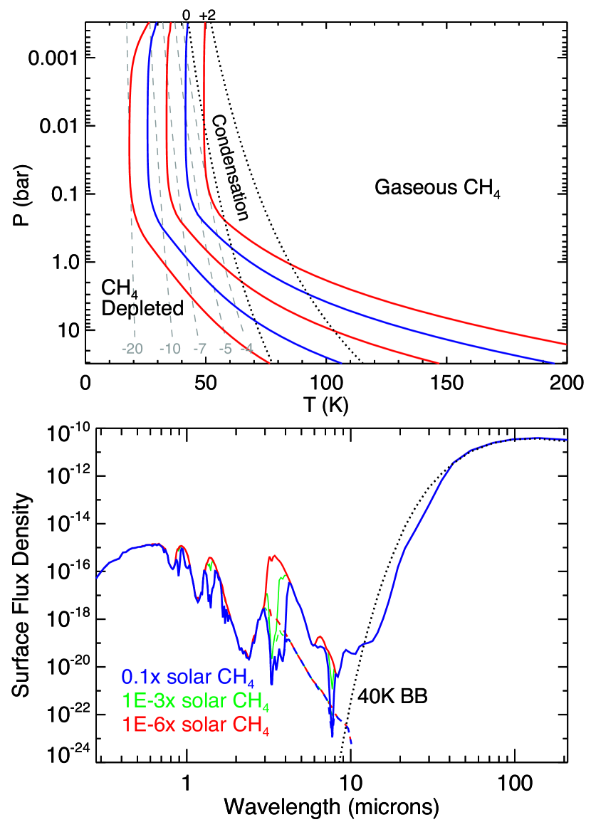
Figure 1.— Top: Model P–T profiles for Planet Nine, assuming solar flux at 622 AU, with methane (CH₄) depleted to 0.1$\times$ the solar abundance. The five profiles assume $T_{\rm int}$=60, 50, 40, 30, and 20 K, right to left, and do not include cloud opacity. In dotted black curves are condensation curves for two abundances of methane: 100$\times$ solar (+2) and solar (0). To the right, methane is found in the gas phase, while to the left, the mixing ratio of gaseous methane is severely depleted, following the iso-abundance curves in gray, showing gaseous CH₄ mixing ratio. A cloud of condensed methane will form in this intermediate region. Bottom: Model spectra (erg s^-1 cm^-2 Hz^-1, at the top of the atmosphere) from the optical to far infrared for three $T_{\rm int}$$=40$ K nominal models at 622 AU and with thick atmospheres and no surface. The dramatic change in spectra due to methane condensation is shown, as methane is depleted at 0.1, 10^-3, and 10${}^{-6}\times$ solar. In the most depleted model, all absorption features are due to H₂ CIA opacity. The scattered light component is shown as dashed curves. A 40 K blackbody is shown as the black dotted curve. Note the tremendous enhancement in thermal fluxes above blackbody values at $\sim$3-5 $\mu$m.

The spectra of these cold atmospheres with and without methane opacity are shown in Figure 1b for a $T_{\rm int}$$=40$ K model, representing the expected upper-limit of the flux from a 10 $M_{\oplus}$model. The optical spectrum is nearly feature-free, except for H₂ CIA opacity at 0.8 $\mu$m and possibly methane, if present. The profiles differ by a factor of $10^{5}$ in the methane abundance, which is allowed given the wide-range potential P–T profiles. In the mid-infrared, H₂ CIA and methane are the dominant absorbers, and the presence or absence of methane dramatically alters the spectra. In particular the thermal fluxes from $\sim 3-5$ $\mu$m are enhanced by around 20 orders of magnitude compared to blackbody expectations. All absorption features in the red model spectrum are due to H₂ CIA. In addition, the loss of methane opacity shifts a prominent flux maximum from 4+ $\mu$m to $\sim 3-3.5$ $\mu$m, which dramatically alters the flux ratio in the two shortest WISE and Spitzer bands. Tabulated thermal infrared magnitudes are given in Table 2.

Our previously mentioned uncertain opacities at low temperature lead to some qualifications on our conclusions. A strong enhancement of flux from 3-5$\mu$m is robust. The large H₂ CIA opacities at tens of microns, with a pronounced minimum at 3-4 $\mu$m, is a generic outcome at any temperature (e.g. Sharp & Burrows, 2007, Figure 15), which forces flux into these opacities windows, as is well understood in brown dwarf and giant planet atmospheres. However, quantitatively, the shape of the emitted spectra certainly do depend on specifics of the absorption coefficients. An addition, we do not include the effects of the hypothesized, and potentially optically thick (at least at short wavelengths) CH₄ cloud, given the large uncertainties on its location and optical properties. This could depress the 3-5 $\mu$m flux compared to the cloud-free case, which emerges from deep, hotter atmospheric layers. Even with potentially dramatic flux enhancements, given the faintness of the planet in the mid-infared, we expect that in the near future a detection in the optical is the most likely, and we next turn to what information may be gleaned from an optical spectrum.

$T_{\rm eff}$	CH4	u	g	r	i	z	Y	VR	Y	J	H	K	L’	M’	W1	W2	W3	W4
(K)	abund
20	10-1	22.3	22.0	21.4	22.4	22.1	23.0	21.5	23.4	24.4	23.9	31.0	29.4	29.9	27.6	29.3	35.5	26.4
20	10-3	22.3	22.0	21.3	22.3	21.3	21.9	21.5	22.4	23.9	23.4	30.9	28.1	29.9	27.1	29.3	36.4	29.6
20	10-6	22.3	22.0	21.3	22.3	21.2	21.8	21.5	22.3	23.8	23.4	30.9	27.1	29.9	26.0	29.3	36 .3	29.6
30	10-1	22.3	22.0	21.4	22.4	22.2	23.0	21.5	23.3	24.3	24.0	30.8	29.5	29.7	27.4	29.0	31.9	19.8
30	10-3	22.3	22.0	21.3	22.2	21.3	21.8	21.4	22.3	23.8	23.5	30.7	27.9	29.7	26.9	28.9	31.9	19.8
30	10-6	22.3	22.0	21.3	22.2	21.2	21.8	21.4	22.2	23.7	23.5	30.7	26.4	29.7	25.6	28.9	31.9	19.8
40	10-1	22.3	22.0	21.4	22.3	22.2	22.9	21.5	23.3	24.3	24.1	30.6	26.0	23.9	27.6	23.2	25.4	14.2
40	10-3	22.3	22.0	21.3	22.2	21.4	21.9	21.4	22.3	23.9	23.7	30.6	22.4	23.9	23.9	22.8	25.4	14.2
40	10-6	22.3	22.0	21.3	22.2	21.3	21.8	21.4	22.3	23.8	23.6	30.6	20.5	23.9	20.5	22.8	25.4	14.2
50	10-1	22.3	22.0	21.4	22.3	22.3	23.0	21.5	23.3	24.4	24.5	30.5	21.1	17.7	28.0	17.6	20.0	10.6
50	10-3	22.3	22.0	21.3	22.1	21.5	22.0	21.4	22.4	24.0	23.9	30.5	17.3	17.7	19.0	17.2	20.0	10.6
50	10-6	22.3	22.0	21.3	22.1	21.4	21.9	21.4	22.3	24.0	23.9	30.5	15.8	17.7	16.1	17.2	20.0	10.6
60	10-1	22.3	22.0	21.4	22.2	22.5	23.1	21.5	23.4	24.6	24.9	30.4	18.0	13.5	27.5	13.7	15.9	8.1

Note. — Apparent magnitudes at 622 AU (see Fienga et al., 2016), using the described cloud-free atmosphere models and the radius of Neptune. The first seven filters are for DECcam (u to VR), the next five or MKO filters, while the last four are for WISE (W1 to W4). L’ band and redder are dominated by thermal emission, which is dominated by intrinsic flux and therefore does not depend on the orbital separation, while shorter wavelength bands are dominated by solar reflection. Therefore these thermal vs. reflected magnitudes will change as a function of orbital distance in different ways.

4. Optical Characterization

Because any atmosphere of Planet Nine will be cold and may be relatively “clean” compared to solar system analogs, the reflection spectrum may well have some counter-intuitive characteristics, which we discuss below. In Figure 2 we present a notional geometric albedo spectrum of a planet such as modeled here to help motivate early characterization efforts.

The geometric albedo of an infinitely deep Rayleigh scattering albedo is 0.75 at all wavelengths. (See Marley et al., 1999, for a discussion of the various forms of albedo and limiting cases.) Thus the scattered light spectrum from a deep, mostly $\rm H_{2}-He$ atmosphere would primarily be a mirror of that of the sun. At UV wavelengths, however, Raman scattering by $\rm H_{2}$ becomes important (e.g., Marley et al., 1999; Oklopčić et al., 2016) and will depress the geometric albedo (to as low as $\sim 0.6$). But at longer wavelengths where the Rayleigh cross section is high and Raman less important, $\sigma_{\rm Ray}\approx{\sigma_{0}}\lambda^{-4}$ (where $\sigma_{0}=8.14\times 10^{-17}$ with $\lambda$ in nm), is large and the photochemical hazes that darken the UV and blue spectra of solar system giants will likely be sparse or absent (owing to the faint UV flux and the paucity of methane). If there is, however, a bright $\rm CH_{4}$ cloud deck then we would expect the geometric albedo to transition from the pure Rayleigh value in the blue to a value controlled by Mie scattering from the cloud deck at a wavelength $\lambda_{\rm R}$ where the column two-way Rayleigh scattering optical depth, averaged over the disk, is about 1: $2\tau_{\rm Ray}/{\bar{\mu}}\approx 1$. Assuming hydrostatic equilibrium in an approximately isothermal atmosphere and setting $\bar{\mu}=0.5$ we have

$$\lambda_{\rm R}=\Bigl{(}{4\sigma_{0}{P_{c}}\over mg}\Bigr{)}^{1/4},$$ (1)

where $m$ is the mean molecular weight of the atmosphere and $g$ is the gravity, yielding $\lambda_{\rm R}$ in nm. For a cloudtop at 10 bar and $g=800\,\rm cm^{2}/s)$, $\lambda_{\rm R}=400\,\rm nm$. Whether the cloud is brighter or darker than the overlying Rayleigh atmosphere depends on its column mass, particle size, and vertical abundance profile. Thus Figure 2 illustrates both a brighter and darker cloud influencing the spectra at $\lambda>\lambda_{\rm R}$. Regardless, a break in the slope of the scattered light spectrum thus provides a measure of the cloud top altitude, which helps to constrain the atmosphere’s thermal profile (see Figure 1a).

We also expect (Figure 1b) that there may well be some absorption features evident in a reflected light spectrum of the planet, including pressure-induced absorption features from $\rm H_{2}-H_{2}$ and $\rm H_{2}-He$ at $\sim~{}0.8\,\rm\mu m$. The depth of the features will depend upon the column of gas above the cloud. For deep, cloudless atmospheres these features could be quite deep and broad. Finally gaseous CH₄ absorption above the cloud deck will produce the usual “giant planet” methane bands, although given the low temperatures and the expected small column above the cloud it is may that in the optical only the strongest band, at $0.889\,\rm\mu m$ will be prominent. The colder the atmosphere, the deeper the cloud, the redder $\lambda_{\rm R}$, and the lower the mixing ratio of gaseous methane in the observable atmosphere. The use of the CH₄ mixing ratio as a “atmospheric thermometer” could be complicated since the mixing ratio will be a strong function of temperature (and hence, depth) in the atmosphere (Figure 1a). This could necessitate the detection multiple bands of CH₄ (into the near IR). These bands would be of different inherent strengths, which would become optically thick at different atmospheric depths, which could yield a full picture of the CH₄ mixing ratio with depth.

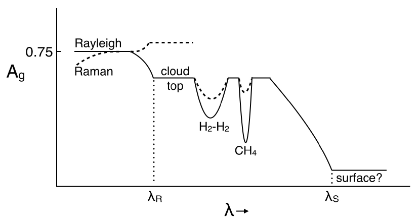
Figure 2.— Notional geometric albedo spectrum across the optical to near infrared illustrates the expected key influences on the reflected light spectrum. For a deep H₂ atmosphere most atmospheric opacity is due to Rayleigh scattering, but since the cross-section falls off as $\lambda^{-4}$, one sees progressively deeper at redder wavelengths. At some wavelength $\lambda_{\rm R}$ one sees photons that reflect off of the top of the CH₄ cloud, which could be brighter (dashed) or darker than a purely Rayleigh scattering atmosphere. The band depths due to H₂ and CH₄ depend, as illustrated by the dashed lines, on the column density above the cloud and the gravity. At even longer wavelengths, Mie cloud opacity lessens, and there could be reflection from a planetary surface beyond $\lambda_{\rm S}$. At the bluest wavelengths Raman scattering by H₂ molecules may be important, reducing the geometric albedo below the pure Rayleigh limit of 0.75.

If there is a solid surface, then at some wavelength, $\lambda_{\rm S}$, the scattered light albedo will be dominated by the properties of the surface. For Mie scattering particles the extinction cross section drops precipitously for wavelengths greater than about 10 times the mean particle radius. Thus for a cloud consisting of submicron particles, near-infrared flux may penetrate both the cloud and the scattering gas, assuming the surface pressure is not too great. The windows through which the deep atmosphere of Venus and the surface of Titan are glimpsed through haze and gas are examples of this effect. The wavelength of such a break at which the surface becomes detectable, if observed, provides a measure of the surface pressure $\lambda_{\rm S}\propto P_{\rm s}^{1/4}$.

5. Detectability

With its expected eccentricity of order $e=0.6$, and a posited semi-major axis of order $a=700\,{\rm AU}$, Planet Nine’s reflected light visual magnitude would vary by a factor of $((1+e)/(1-e))^{4}=256$ over the course of its orbit. As a consequence, its detectability is strongly influenced by its current radial distance from the Sun, which, as a function of true anomaly, $\nu$, is given by

$$r_{P9}=\frac{a(1-e^{2})}{(1+e\cos\nu)}\,.$$ (2)

Planet Nine’s V-band magnitude, therefore, is

$$V_{P9}=7.8+5\log_{10}\left[\left(\frac{R_{\rm P9}}{R_{\rm Nep}}\right)^{2}\left(\frac{A_{\rm P9}}{A_{\rm Nep}}\right)\left(\frac{r_{P9}}{29\,{\rm AU}}\right)^{4}\right]\,,$$ (3)

where $V_{\rm N}=7.8$ is Neptune’s visual magnitude at opposition, and Neptune’s geometric albedo is taken as $A_{\rm Nep}=0.41$.

As a concrete illustration, consider the fiducial 10 $M_{\oplus}$ Planet Nine candidate proposed by Batygin & Brown (2016), in conjunction with the orbital location obtained by Fienga et al. (2016) that provides the maximum reduction of the Cassini residuals. These assumptions lead to orbital elements: $a=700\,{\rm AU}$, $e=0.6$, $i=30^{\circ}$, $\omega=150^{\circ}$, $\Omega=113^{\circ}$, and $\nu=118^{\circ}$, where $i$ is the inclination to the ecliptic, $\omega$ is the argument of perihelion, and $\Omega$ is the longitude of the planet’s ascending node. These elements correspond to a sky position of R.A.$\,\sim 2\,{\rm hr}$, Dec$\,\sim-20^{\circ}$ in the constellation Cetus, and imply a current distance $r_{\rm P9}=622\,{\rm AU}$. In addition, if we adopt a Neptune-like envelope mass fraction of $f_{\rm env}=M_{\rm atm}/M_{\rm pl}=0.1$, our structural model suggests $R_{\rm P9}=3.46\,R_{\oplus}$. Drawing on the results of §4, we adopt a geometric albedo $A_{\rm P9}=0.75$, which generates a current visual magnitude V=21.6. In the event that it has these parameters, Planet Nine would be detectable in the optical by the ongoing Dark Energy Survey, which is sensitive in the relevant sky location to $r<23.8$ (Brown & Batygin, 2016).

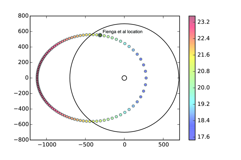
Figure 3.— Planet Nine orbit with the position of the planet shown at 100 equally spaced time intervals. Color is tied to expected V magnitude, as computed with the atmospheric models of the previous section. The 700 AU semi-major axis is indicated by the black solid line. The best-fit location derived by Fienga et al. (2016) is shown as a black dot.

If considered as a 40K blackbody radiator, Planet Nine’s thermal spectrum peaks at $\lambda\sim 70\,\mu{\rm m}$, rendering its detection difficult, but potentially possible, with present-day space-based instrumentation and survey coverage.

Ginzburg et al. (2016) adopt a primarily analytic approach to infer the current planetary surface temperature from the mass and composition of the planet. Using a two-component model for the core-envelope structure of the planet, they show that some of the mass-composition parameter space (assuming a black body spectrum) is accessible to the NASA WISE Mission’s W4 (22 $\mu$m) bandpass, and find that for a bulk composition with $f_{\rm env}=M_{\rm atm}/M_{\rm pl}=0.1$, and $R_{\rm pl}=1.2~{}R_{\rm Nep}$, Planet Nine is potentially detectable by WISE at an $r_{P9}\sim a\sim$700 AU distance.

The models delineated in Table 2 indicate that Planet Nine might be much brighter in the W1 (3.4 $\mu$m) WISE band than its effective temperature would otherwise suggest. Our extremal case, with $T_{\rm eff}=50~{}{\rm K}$ and $10^{-6}\,{\rm CH_{4}}$ abundance, predicts W1=16.1, which exceeds the WISE All-Sky 5$\sigma$ sensitivity limit of W1=16.5 (Wright et al., 2010) for static object flux measurements obtained by co-adding individual source frame images. For W1 and W2, these limits were substantially improved (for stationary sources) through the incorporation of post-cryo NEOWISE observations as well as by data processing improvements (Mainzer et al., 2011). On the other hand, an object that moves significantly between epochs would contribute all of its flux to a given catalogued point source during a single epoch. For example, if P9 with intrinsic W1=16.11 were to contribute to half of the frames in a co-added two-epoch image, its reported W1 would be $\sim$0.75 magnitudes fainter than its true W1.

At the nominal Fienga et al. (2016) location of R.A.$\,\sim 2\,{\rm hr}$, Dec$\,\sim-20^{\circ}$, Planet Nine’s total annual parallax shift would be of order $\pi=663{{}^{\prime\prime}}$, and its yearly positional shift on the sky arising from its orbital motion would be of order $\sigma\sim 60{{}^{\prime\prime}}\,{\rm yr^{-1}}$. These displacements combine to yield a maximum sky motion of $\delta\lesssim 6{{}^{\prime\prime}}\,{\rm day^{-1}}$. Given WISE’s sun-synchronous geocentric orbit and Planet Nine’s current nominal angular parameters ($i=30^{\circ}$, $\Omega=113^{\circ}$, and $\nu=118^{\circ}$), its expected angular sky motion at the epochs of observation would be $\dot{\pi}\sim 0.12^{\prime\prime}{\,\rm hr}^{-1}$, or $\Delta\pi=2.3^{\prime\prime}$ over the 4/5th day observing sequence that is expected at Planet Nine’s current ecliptic latitude. This estimate for $\Delta\pi$ is smaller than WISE’s W1 FWHM resolution of 6.1^′′. As a consequence, any WISE detection of Planet Nine in the AllWISE point source catalog should register as a series of several fully separated W1-detected (and possibly W2-detected) objects lying within a roughly one square arc minute region of the sky. These separate appearances of Planet Nine, in turn, will each be drawn from roughly twelve single-exposure images taken during a $\sim$4/5 day period covered by overlapping scans; for further details see Wright et al. (2010).

We filtered the AllWISE Source Catalog for objects with $0~{}{\rm h}<{\rm RA}<4~{}{\rm h}$ and $-30^{\circ}<{\rm Dec}<0^{\circ}$, having W1$>$16, W2$>$17 (or null), W3$>20$ (or null), and W4$>$10 (or null). This screen produced a single match: J005009.06 -315732.2 (J005), which has W1=16.972 and W2=17.032, and which was observed by WISE on 5 individual image frames. The WISE catalog reports that J005’s W1 timestamps span a single 2-day period from HJD 2455542.53 through 2455546.16. Based on the foregoing discussion, a single-source detection built up over 4 days is at best marginally consistent with Planet Nine’s expected sky movement. The J005 object is not, furthermore, paired with any sources having similar photometry in the near vicinity and at separate epochs. Moreover, J005’s W2 single-frame detection epochs range over a 6-month span from HJD 2455365.12 to HJD 2455546.16, implying that it is a transiently detected, yet nonetheless stationary object or noise source. J005 can therefore confidently be rejected from consideration as a Planet Nine candidate. While we believe it is exceedingly unlikely that Planet Nine can be located in the AllWISE Source Catalog, it is unlikely yet nonetheless possible that it makes an appearance in the AllWISE Reject Table. We are currently sifting this 428,787,253-line database for candidates.

6. Conclusions

We have modeled several aspects of the thermal evolution and atmospheric structure and spectra of the possible Planet Nine. Like others, we find a planetary $T_{\rm eff}$ of perhaps $35-50$ K, depending on mass, but we caution that these are upper limits. The atmosphere could well be in a temperature range of significant condensation of methane. The loss of this important “giant planet” opacity source can dramatically alter both the reflection and emission spectra away from expectations based on Uranus and Neptune, with the notable effect of causing Planet Nine to appear “blue” rather than “red” in the WISE bands.

Our models suggest that the reflection spectrum, due to a mix of Rayleigh scattered sunlight, cloud scattering, and absorption due to H₂ and CH₄ opacity could provide rich diagnostics of the temperature structure, possible cloud location, and even surface pressure of the atmosphere. Let the hunt continue.

References

- Batygin & Brown (2016) Batygin, K., & Brown, M. E. 2016, AJ, 151, 22
- Becker et al. (2014) Becker, A., Lorenzen, W., Fortney, J. J., et al. 2014, ApJS, 215, 14
- Borucki et al. (2011) Borucki, W. J., Koch, D. G., Basri, G., et al. 2011, ApJ, 728, 117
- Bromley & Kenyon (2016) Bromley, B. C., & Kenyon, S. J. 2016, ArXiv e-prints, arXiv:1603.08010
- Brown & Batygin (2016) Brown, M. E., & Batygin, K. 2016, ArXiv e-prints, arXiv:1603.05712
- Cowan et al. (2016) Cowan, N. B., Holder, G., & Kaib, N. A. 2016, ApJ, 822, L2
- de la Fuente Marcos & de la Fuente Marcos (2016) de la Fuente Marcos, C., & de la Fuente Marcos, R. 2016, MNRAS, 459, L66
- Fienga et al. (2016) Fienga, A., Laskar, J., Manche, H., & Gastineau, M. 2016, A&A, 587, L8
- Fortney et al. (2008) Fortney, J. J., Lodders, K., Marley, M. S., & Freedman, R. S. 2008, ApJ, 678, 1419
- Fortney et al. (2007) Fortney, J. J., Marley, M. S., & Barnes, J. W. 2007, ApJ, 659, 1661
- Fortney & Nettelmann (2010) Fortney, J. J., & Nettelmann, N. 2010, Space Sci. Rev., 152, 423
- Freedman et al. (2014) Freedman, R. S., Lustig-Yaeger, J., Fortney, J. J., et al. 2014, ApJS, 214, 25
- Ginzburg et al. (2016) Ginzburg, S., Sari, R., & Loeb, A. 2016, ApJ, 822, L11
- Graboske et al. (1975) Graboske, H. C., Olness, R. J., Pollack, J. B., & Grossman, A. S. 1975, ApJ, 199, 265
- Guillot et al. (1995) Guillot, T., Chabrier, G., Gautier, D., & Morel, P. 1995, ApJ, 450, 463
- Helled et al. (2011) Helled, R., Anderson, J., Podolak, M., & G., S. 2011, ApJ, 726, A15
- Holman & Payne (2016) Holman, M. J., & Payne, M. J. 2016, ArXiv e-prints, arXiv:1603.09008
- Hubbard & Marley (1989) Hubbard, W. B., & Marley, M. S. 1989, Icarus, 78, 102
- Hubbard et al. (1995) Hubbard, W. B., Podolak, M., & Stevenson, D. J. 1995, in Neptune and Triton, ed. Cruishank (University of Arizona, Tucson), 109–138
- Kenyon & Bromley (2016) Kenyon, S. J., & Bromley, B. C. 2016, ArXiv e-prints, arXiv:1603.08008
- Li & Adams (2016) Li, G., & Adams, F. C. 2016, ApJ, 823, L3
- Linder & Mordasini (2016) Linder, E. F., & Mordasini, C. 2016, A&A, 589, A134
- Lopez & Fortney (2014) Lopez, E. D., & Fortney, J. J. 2014, ApJ, 792, 1
- Mainzer et al. (2011) Mainzer, A., Bauer, J., Grav, T., et al. 2011, ApJ, 731, 53
- Malhotra et al. (2016) Malhotra, R., Volk, K., & Wang, X. 2016, ArXiv e-prints, arXiv:1603.02196
- Marley et al. (2007) Marley, M. S., Fortney, J. J., Hubickyj, O., Bodenheimer, P., & Lissauer, J. J. 2007, ApJ, 655, 541
- Marley et al. (1999) Marley, M. S., Gelino, C., Stephens, D., Lunine, J. I., & Freedman, R. 1999, ApJ, 513, 879
- Marley & McKay (1999) Marley, M. S., & McKay, C. P. 1999, Icarus, 138, 268
- Marley et al. (2012) Marley, M. S., Saumon, D., Cushing, M., et al. 2012, ApJ, 754, 135
- Marley et al. (1996) Marley, M. S., Saumon, D., Guillot, T., et al. 1996, Science, 272, 1919
- McKay et al. (1989) McKay, C. P., Pollack, J. B., & Courtin, R. 1989, Icarus, 80, 23
- Morley et al. (2014) Morley, C. V., Marley, M. S., Fortney, J. J., et al. 2014, ApJ, 787, 78
- Mustill et al. (2016) Mustill, A. J., Raymond, S. N., & Davies, M. B. 2016, MNRAS, arXiv:1603.07247
- Nettelmann et al. (2013) Nettelmann, N., Helled, R., Fortney, J. J., & Redmer, R. 2013, Planet. Space Sci., 77, 143
- Oklopčić et al. (2016) Oklopčić, A., Hirata, C. M., & Heng, K. 2016, ArXiv e-prints, arXiv:1605.07185
- Sharp & Burrows (2007) Sharp, C. M., & Burrows, A. 2007, ApJS, 168, 140
- Visscher et al. (2010) Visscher, C., Lodders, K., & Fegley, Jr., B. 2010, ApJ, 716, 1060
- Wright et al. (2010) Wright, E. L., Eisenhardt, P. R. M., Mainzer, A. K., et al. 2010, AJ, 140, 1868