Ultrafast many-body interferometry of impurities coupled to a Fermi sea
Abstract
The fastest possible collective response of a quantum many-body system is related to its excitations at the highest possible energy. In condensed-matter systems, the corresponding timescale is typically set by the Fermi energy. Taking advantage of fast and precise control of interactions between ultracold atoms, we report on the observation of ultrafast dynamics of impurities coupled to an atomic Fermi sea. Our interferometric measurements track the non-perturbative quantum evolution of a fermionic many-body system, revealing in real time the formation dynamics of quasiparticles and the quantum interference between attractive and repulsive states throughout the full depth of the Fermi sea. Ultrafast time-domain methods to manipulate and investigate strongly interacting quantum gases open up new windows on the dynamics of quantum matter under extreme non-equilibrium conditions.
Non-equilibrium dynamics of fermionic systems is at the heart of many problems in science and technology, from the physics of neutron stars and heavy ion collisions to the operation of electronic devices. The wide range of energy scales, spanning the low energies of excitations near the Fermi surface up to high energies of excitations from deep within the Fermi sea, challenges our understanding of the quantum dynamics in such fundamental systems. The Fermi energy sets the shortest response time for the collective response of a fermionic many-body system through the Fermi time , where is the reduced Planck constant. In a metal, i.e. a Fermi sea of electrons, is in the range of a few electronvolts, which corresponds to on the order of 100 attoseconds. Dynamics in condensed matter systems on this timescale can be recorded by attosecond streaking techniques Krausz and Ivanov (2009) and the initial applications were demonstrated by probing photoelectron emission from a surface Pazourek et al. (2015). However, despite these spectacular advances, the direct observation of the coherent evolution of a fermionic many-body system on the Fermi timescale has remained beyond reach.
In atomic quantum gases, the fermions are much heavier and the densities far lower, which brings into the experimentally accessible range of typically a few microseconds. Furthermore, the powerful techniques of atom interferometry Cronin et al. (2009) now offer the exciting opportunity to probe and manipulate the real-time coherent evolution of a fermionic quantum many-body system. Such techniques have been successfully used, e.g. to measure bosonic Hanbury-Brown-Twiss correlations Simon et al. (2011), demonstrate topological bands Atala et al. (2013), probe quantum and thermal fluctuations in low-dimensional condensates Gring et al. (2012); Hadzibabic et al. (2006), and to measure demagnetization dynamics of a fermionic gas Koschorreck et al. (2013); Bardon et al. (2014). Impurities coupled to a quantum gas provide a novel and unique probe of the many-body state. Strikingly, they allow direct access to the system’s wave function when the internal states of the impurities are manipulated using a Ramsey atom-interferometric technique Goold et al. (2011); Knap et al. (2012).
We employ dilute 40K atoms in a 6Li Fermi sea to measure the response of the sea to a suddenly introduced impurity. For near-resonant interactions, we observe coherent quantum many-body dynamics involving the entire 6Li Fermi sea. We also observe in real time the formation dynamics of the repulsive and attractive impurity quasiparticles. In the limit of low impurity concentration, our experiments confirm that an elementary Ramsey sequence is equivalent to linear-response frequency-domain spectroscopy. We demonstrate that our time-domain approaches allow us to prepare, control, and measure many-body interacting states.
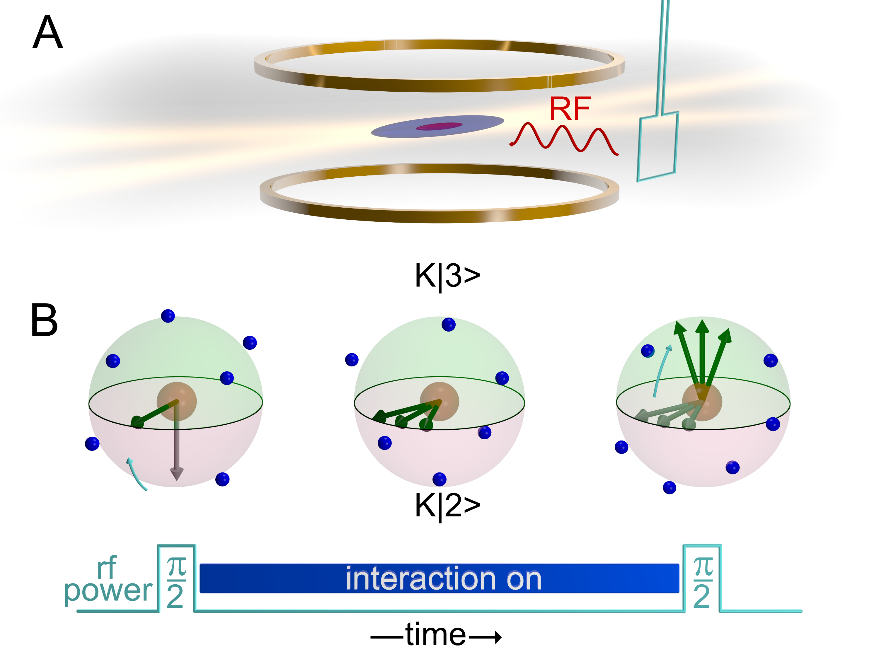
Our system consists of a small sample of typically 40K impurity atoms immersed in a Fermi sea of 3 6Li atoms Cetina et al. (2015); sup . The mixture is held in an optical dipole trap (Fig. 1A) at a temperature of nK after forced evaporative cooling. Because of the Li Fermi pressure and a more than two times stronger optical potential for K, the K impurities are concentrated in the central region of the large Li cloud. Here they experience a nearly homogeneous environment with an effective Fermi energy of K sup , where is Boltzmann’s constant. The corresponding Fermi time s sets the natural time scale for our experiments. The degeneracy of the Fermi sea is characterized by . The concentration of K in the Li sea remains low, with , where () is the average of the Li (K) number density sampled by the K atoms sup .
The interaction between the impurity atoms in the internal state K (third-to-lowest Zeeman sublevel) and the Li atoms (always kept in the lowest Zeeman sublevel) is controlled using a rather narrow sup interspecies Feshbach resonance near a magnetic field of 154.7 G Naik et al. (2011); Cetina et al. (2015). We quantify the interaction with the Fermi sea by the dimensionless parameter , where is the Li Fermi wavenumber with the Li mass, and is the -wave interspecies scattering length. While slow control of is realized in a standard way by variations of the magnetic field, fast control is achieved using an optical resonance shifting technique Cetina et al. (2015). The latter permits sudden changes of by up to about within a time shorter than ns.
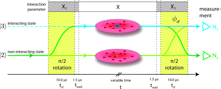
Our interferometric probing method is based on a two-pulse Ramsey scheme (Fig. 1B), following the suggestions of Refs. Goold et al. (2011); Knap et al. (2012). The sequence starts with the impurity atoms prepared in the spin state K (second-to-lowest Zeeman sublevel), for which the background interaction with the Fermi sea can be neglected. A first, 10-s-long, radio-frequency (rf) -pulse drives the K atoms into a coherent superposition between this non-interacting initial state and the state K under weakly interacting conditions (interaction parameter with ). Using the optical resonance shifting technique Cetina et al. (2015), the system is then rapidly quenched into the strongly interacting regime (). After an evolution time , the system is quenched back into the regime of weak interactions and a second -pulse is applied. The population difference in the two impurity states is measured as a function of the phase of the rf pulse Cetina et al. (2015). The contrast and the phase of the resulting sinusoidal signal is finally determined as a function of . In the limit of low impurity concentration, the complex function can be interpreted as the overlap of the interacting and the non-interacting components of the system’s wavefunction Goold et al. (2011). The squared amplitude is then equivalent to the common definition of a Loschmidt echo Loschmidt (1876); Jalabert and Pastawski (2001).
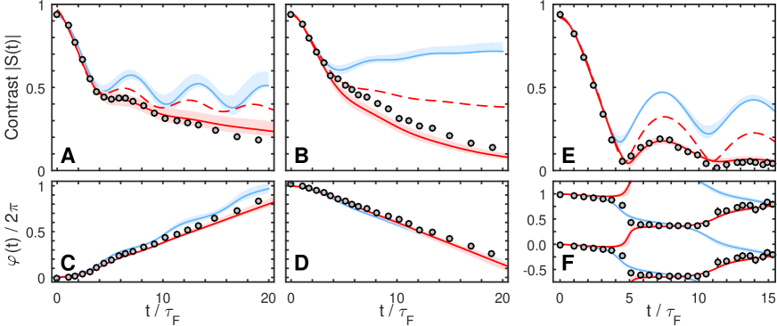
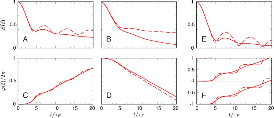
We first consider the interaction conditions where polaronic quasiparticles are known to exist Massignan et al. (2014). Figures 2A-D show the evolution of the contrast and the phase measured in the repulsive and the attractive polaron regimes, where and , respectively. For short evolution times of up to about , we observe both contrast signals to exhibit a similar initial parabolic transient, which is typical of a Loschmidt echo Jalabert and Pastawski (2001). For longer times, this connects to an exponential decay of the contrast and a linear evolution of the phase. In Ref. Cetina et al. (2015), we showed that the long-time decay of the contrast in this regime can be interpreted in terms of quasiparticle scattering. Here, the linear phase evolution corresponds to the energy shift of the quasiparticle state, for which we obtain for the repulsive case in Fig. 2C and for the attractive case in Fig. 2D. Remarkably, while the long-time behavior reflects the quasiparticle properties, the observed initial transient reveals the ultrafast real-time dynamics of the quasiparticle formation.
On resonance, for the strongest possible interactions, the quasiparticle picture breaks down. Here our measurements, displayed in Fig. 2E and 2F for = 0.08(5), reveal the striking quantum dynamics of a strongly interacting fermionic system forced into an extreme non-equilibrium state. The contrast shows pronounced oscillations reaching zero, while the phase exhibits plateaus. The revivals of the contrast indicate partially reversible entanglement between the internal state of the impurity and the Fermi sea Goold et al. (2011). This process involves the whole Fermi sea and occurs on the fastest timescale available to the collective dynamics of a fermionic system.
To further interpret our measurements we employ two different theoretical approaches: the truncated basis method (TBM) sup and the functional determinant approach (FDA) Knap et al. (2012). The TBM models our full experimental procedure assuming zero temperature and considering only single particle-hole excitations. This approximation, known as the Chevy ansatz Chevy (2006), has been successfully used to predict the properties of quasiparticles in cold gases Massignan et al. (2014). The predictions of the TBM are represented by the blue lines in Fig. 2. This method accurately describes the initial transient, as well as the period of the oscillations of on resonance. While the zero-temperature TBM calculation naturally overestimates the contrast in the thermally dominated regime (), it accurately reproduces the observed linear phase evolution and thus the quasiparticle energy. The FDA is an exact solution for a fixed impurity at arbitrary temperatures taking into account the non-perturbative creation of infinitely many particle-hole pairs. The FDA calculation is represented by the solid red lines in Fig. 2. We see remarkable agreement with our experimental results, which indicates that the effects of impurity motion remain small in our system. This observation can be explained by the fact that our impurity is sufficiently heavy so that the effects of its recoil with energies of about sup are masked by thermal fluctuations. To identify the effect of temperature, we performed a corresponding FDA calculation for and show the results as the dashed lines in Fig. 2. Here, we see a slower decay of , which follows a power law at long times sup under the idealizing assumption of infinitely heavy impurities.
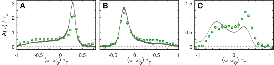
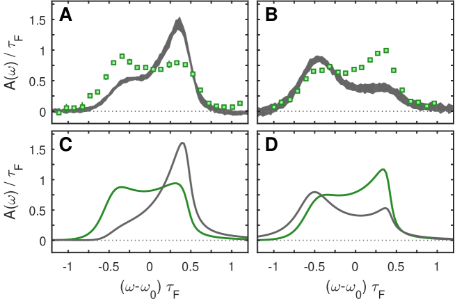
Time-domain and frequency-domain methods are closely related, as is well known in spectroscopy. In the limit of low impurity density, where the interactions between the impurities can be neglected, is predicted to be proportional to the inverse Fourier transform of the linear excitation spectrum of the impurity Nozières and de Dominicis (1969). To benchmark our interferometric method, we measure using rf spectroscopy similar to our earlier work Kohstall et al. (2012), but with great care to ensure linear response sup . The measured excitation spectra are shown in Fig. 3. In the repulsive and attractive polaron regimes, we observe the characteristic structure of a peak on top of a broad pedestal Massignan et al. (2014). While the peak determines the long-time evolution of the quasiparticle, the pedestal is associated with the rapid dynamics related to the emergence of many-body correlations. For resonant interactions, the rf response is broad and nearly symmetric about , implying that the zero crossings of are accompanied by jumps in its phase by , as is seen in Fig. 2E and 2F. Based on the observed spectral response, we interpret the oscillations of in Figs. 2E and 2F as arising from simultaneous excitations of the two branches of our many-body system corresponding to the two humps in the rf spectrum.
A detailed comparison of our time- and frequency-domain measurements reveals the powerful capability of our approach to prepare and control many-body states. This is revealed in Fig. 3, where we show the Fourier transform of the data from Fig. 2 as the gray curves. We observe that time-domain measurements where the rf pulses are applied in the presence of weakly repulsive interactions (Fig. 3A) emphasize the upper branch of the many-body system while in the attractive case (Fig. 3B,C), the lower branch is emphasized. We explain this observation by the action of the rf pulses to prepare weakly interacting polaron states sup . Compared to the non-interacting initial state used in the frequency-domain spectroscopy, these polarons have an increased wavefunction overlap with the corresponding strongly interacting repulsive and attractive branches, leading to the observed shift in the spectral weight. Our measurements demonstrate that the control over the initial state of many particles can be used to precisely manipulate quantum dynamics in the strongly interacting regime. This unique capability of time-domain techniques opens up a wide range of applications, including the study of the dynamical behavior near the phase transition from a polaronic to a molecular system Massignan et al. (2014) and the creation of specific excitations of a Fermi sea down to individual atoms Dubois et al. (2013).
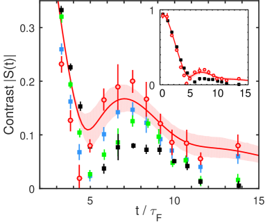
Our interpretation of the results in Figs. 2 and 3 relies on the assumption that our fermionic impurities are sufficiently dilute so that any interactions between them can be neglected. We can extend our experiments into a complex many-body regime where the impurities interact both with the Fermi sea and with each other, by increasing the impurity concentration sup . Figure 4 shows the time-dependent contrast measured for and 0.20, 0.33, and 0.53. An extrapolation of the data to zero concentration (open red circles) lies close to the data points for 0.20, which is the typical concentration in our measurements, and agrees with the FDA calculation. This confirms that the physics that we access in the measurements with a small sample of fermionic impurities is close to that of a single impurity, which we posit to be a consequence of the fermionic nature of the impurities. When the impurity concentration is increased, we find that the contrast for is decreased and the period of the revivals of is prolonged. We interpret this as arising from effective interactions between the impurities induced by the Fermi sea Mora and Chevy (2010); Yu et al. (2010). Such interactions between fermionic impurities are predicted to lead to novel quantum phases Zwerger (2012).
Our results demonstrate the power of many-body interferometry to study ultrafast processes in strongly interacting Fermi gases in real time, including the formation dynamics of quasiparticles and the extreme non-equilibrium dynamics arising from quantum interference between different many-body branches. Of particular interest is the prospect of observing Anderson’s orthogonality catastrophe Knap et al. (2012); sup by further cooling the Li Fermi sea Hart et al. (2015) while pinning the K atoms in a deep species-selective optical latticeLeBlanc and Thywissen (2007).
Acknowledgements
We thank M. Baranov, F. Schreck, G. Bruun, N. Davidson and R. Folman for stimulating discussions. We acknowledge support by the Austrian Science Fund FWF within the SFB FoQuS (F40-P04). R. S. was supported by the NSF through a grant for the Institute for Theoretical Atomic, Molecular, and Optical Physics at Harvard University and the Smithsonian Astrophysical Observatory. M. K. acknowledges support from Technical University of Munich - Institute for Advanced Study, funded by the German Excellence Initiative and the European Union FP7 under grant agreement 291763. E. D. acknowledges support from Harvard-MIT CUA, NSF Grant No. DMR-1308435, AFOSR Quantum Simulation MURI, the ARO-MURI on Atomtronics, and support from Dr. Max Rössler, the Walter Haefner Foundation, the ETH Foundation, and the Simons Foundation.
Supplementary Materials
S1 Theoretical description
In this section, we summarize the approaches that we developed to theoretically model the results of our interferometric Ramsey experiments. We first discuss the microscopic model that we use to describe the narrow Feshbach resonance of the Li-K mixture, and then we outline how we calculate the time evolution of the system within two approaches: the Truncated Basis Method (TBM) and the Functional Determinant Approach (FDA). In this section, we assume that a ‘perfect quench’ is performed, where the impurity is initially non-interacting with the Fermi sea and there are no interactions during the radio-frequency (rf) pulses. A discussion of the role played by interactions during the rf pulses is deferred to Section S3.
S1.1 Narrow Feshbach resonance model for Li-K mixtures
In our experiment, the K impurities are concentrated in the central region of the Li Fermi gas where they experience a nearly uniform Li environment (see Section S5.A). Hence we consider in our model K impurities that are immersed in a Li Fermi gas of uniform density. The Li-K mixture is prepared at magnetic fields near a closed-channel dominated Feshbach resonance between the Li and K states that occurs near G. The narrow character of this resonance is a consequence of the limited strength of the coupling of atoms in the open channel to a closed-channel molecular state. To describe this system we use the two-channel Hamiltonian
| (1) |
where the first line defines the non-interacting Hamiltonian . Here, is the total system volume, () creates (annihilates) a Li fermion with momentum and single-particle energy , and () creates (annihilates) a K impurity atom in the K state with dispersion , where we define . The closed-channel molecule is created (annihilated) by (). It has the dispersion , and a bare energy relative to the scattering threshold, . Here is the differential magnetic moment between the open and closed channels, and denotes the threshold crossing of the bare molecular state Chin et al. (2010).
Close to the Feshbach resonance, the scattering length diverges and the interaction between the K impurities and the Li atoms is predominantly mediated by exchange of the closed-channel molecule. We therefore neglect the background scattering potential in the open channel Naik et al. (2011). The strength of the coupling between the open and closed channels is given by , and we take a form factor , which accounts for the finite extent of the closed-channel wave function .
The parameters of the model , , , and are fully determined by known experimental parameters. First, the differential magnetic moment has recently been measured to be 2.35(2) MHz/G Cetina et al. (2015). Second, close to resonance, the scattering length may be parametrized as
| (2) |
where is the center of the Feshbach resonance with width G and background scattering length Naik et al. (2011). To connect with our model, we consider the on-shell two-body scattering amplitude , which for the Hamiltonian (1) is given by Schmidt et al. (2012)
| (3) |
where is the reduced mass and is the relative scattering wave vector. Using the low energy expansion , with the effective range, we thus identify
| (4) | ||||
| (5) |
where is the range parameter of the Feshbach resonance Bruun and Pethick (2004); Petrov (2004). Comparing Eqs. (2) and (4) yields
| (6) | ||||
| (7) |
Equation (6) relates , and thus the coupling constant , to the known experimental parameters. The extent of the closed-channel wave function in turn follows by comparing Eq. (7) to the theoretical prediction from quantum defect theory Góral et al. (2004); Szymańska et al. (2005), , where and is the van der Waals length Naik et al. (2011). Thus we obtain . Finally, was obtained in Ref. Cetina et al. (2015), allowing the determination of .
S1.2 Truncated Basis Method
To model a mobile impurity as in the experiment, we consider an approximate wave function for the zero-momentum impurity that incorporates the scattering of a single particle out of the Fermi sea:
| (8) |
Here, the first term on the right hand side describes the product state of the impurity K atom at zero momentum and the ground state of the non-interacting Li Fermi sea , where is the Fermi momentum, which is related to the Fermi energy by . The last two terms correspond, respectively, to the impurity binding a Li atom to form a closed-channel molecule, and the impurity exciting a particle out of the Fermi sea, in both cases leaving a hole behind. When using the TBM, we focus on zero temperature in order to capture the purely quantum evolution of the impurity. For convenience, within this model we also take , which formally requires taking the bare crossing to keep finite. This approximation is justified, as exceeds by about two orders of magnitude.
Truncated wave functions of the form (8) have been used extensively in the study of Fermi polarons in ultracold atomic gases, starting with the work of Chevy Chevy (2006). While most of the previous work has focused on equilibrium properties, recently it has been proposed that these wave functions may be extended to dynamical problems using a variational approach to obtain the equations of motion Parish and Levinsen (2013), for instance to calculate the decay rate of excited states.
Here, we adapt the use of truncated wave functions for the Fermi polaron to the calculation of the dynamical response of the impurity to an interaction quench. For a perfect quench and at zero temperature, the quantity measured in experiment corresponds to the overlap between the interacting and non-interacting states of the system, i.e., we have Goold et al. (2011); Knap et al. (2012)
| (9) |
Here is the initial non-interacting state of energy , and is the state after a quench at time from zero to finite impurity interactions with the Fermi sea. Formally expanding in a complete set of states for the single impurity problem, the Ramsey signal (9) then becomes
| (10) |
where is an eigenstate of the interacting Hamiltonian with energy . However, this requires one to solve the entire problem which is generally not possible for a mobile impurity. Thus, within the Truncated Basis Method (TBM), we restrict the Hilbert space to wave functions of the form (8) and diagonalize the Hamiltonian within this truncated basis. As we shall see, this truncation permits an extremely accurate description of the initial quantum dynamics of the impurity.
For small , we expand to find
| (11) |
with the Fermi time. This reveals that the short-time dephasing dynamics of is completely determined by the two-body properties, which are captured exactly by the TBM. As we will see below, the TBM describes the impurity behavior also beyond the two-body timescale since higher order correlations and multiple particle-hole excitations take longer to build up. Indeed, for a mobile impurity and for sufficiently weak attraction where the attractive polaron is the ground state, the TBM correctly describes the long-time behavior . Here, is the polaron residue (squared overlap with the non-interacting state) and is the polaron energy, which are both accurately determined using a wave function of the form (8) Vlietinck et al. (2013).
With the TBM we consider zero temperature in order to isolate the quantum dynamics of the impurity. To better model the experiment, in principle one can extend the TBM to finite temperature by taking the initial state to be a statistical thermal distribution involving multiple impurity momenta. However, a more convenient approach at finite temperature is described in the next section.
S1.3 Functional Determinant Approach
At times substantially exceeding , the full description of the impurity dynamics requires the inclusion of multiple particle-hole pair excitations as well as the effect of finite temperature, both of which present a theoretical challenge. In order to study and describe both effects, we employ the Functional Determinant Approach (FDA) Levitov et al. (1996); Levitov and Lesovik (1993); Klich (2003); Knap et al. (2012).
In the FDA the impurity is treated as an infinitely heavy object. In this limit, the FDA provides an exact solution of the dynamical many-body problem at arbitrary temperatures and times. The justification of the infinite mass approximation, which will be discussed in more detail in Section S2, is rooted in two observations. First, in our experiment, the mass of the K impurities is much larger than that of the Li atoms (mass ratio ) which constitute the surrounding Fermi gas. Therefore, the recoil energy gained by the K impurities due to the scattering with a Li atom is small. We estimate the typical recoil momentum by averaging over all possible scattering processes on the Fermi surface, yielding . From that we obtain an estimate for the typical recoil energy , which determines a typical time scale , up to which one expects recoil to have a minimal effect on the many-body quantum dynamics, cf. Section S2.2. Second, at times exceeding the thermal time scale , which in our experiment is given by , thermal effects due to the averaging over various statistical realizations become relevant. The resulting thermal fluctuations disrupt the coherent quantum propagation of the impurity, and hence, for times , mask the effect of recoil Rosch (1999).
To a good approximation, we may thus take the limit of infinite impurity mass, which admits the mapping of Eq. (1) onto the bilinear Hamiltonian
| (12) |
Here, is the creation operator of the localized closed channel molecule and the interaction is described by the annihilation of a Li atom converting the empty impurity molecular state into an occupied one. By taking the limit we obtain a modified reduced mass , which differs by a factor of from the experimental one. This needs to be taken into account when identifying the microscopic parameters. To ensure, in particular, that the off-diagonal coupling in Eq. (12) remains of the same strength as in the experiment, a reduced resonance parameter has been used, which we do for all data shown in the main text. Using these identifications, the model Eq. (12) also accurately describes the short-time dynamics as given by Eq. (11), cf. Fig. 2 in the main text.
The calculation of time-resolved, many-body expectation values such as Eq. (9) at arbitrary temperature presents a theoretical challenge. However, for the model (12), we are able to calculate the time-resolved Ramsey response in an exact way using the FDA Klich (2003); Knap et al. (2012). This is based on the observation that for bilinear Hamiltonians thermal expectation values in the many-body Fock space can be reduced to determinants in the single-particle space by virtue of the identity
| (13) |
Here are many-body operators, are their single-particle counterparts, is the many-body density matrix describing the state of the system, and is the occupation operator defined in the single-particle space, with the fermion chemical potential. A specific example for Eq. (13) is the perfect quench Ramsey response, which at finite temperature is given by Knap et al. (2012)
| (14) |
Here, is the free Hamiltonian of the Li Fermi gas and is the Hamiltonian in the presence of impurity scattering given in Eq. (12), while and are their single-particle counterparts. A numerical evaluation of Eq. (14) then only requires a calculation of the single particle orbitals and energies in order to obtain the single-particle determinant.
S2 Role of physical processes on different time scales
The combination of both our theoretical approaches allows us to accurately model the physics at various time scales in our experiment. Making use of the fact that the FDA and the TBM differ distinctly in their treatment of multiple particle-hole excitations, the impurity mass, and finite temperature, we can use a comparison of their predictions to determine the role of these processes and effects in the many-body non-equilibrium dynamics of our experiment. To keep the analysis transparent, in this section we still assume that a perfect quench is performed.
S2.1 Multiple particle-hole excitations
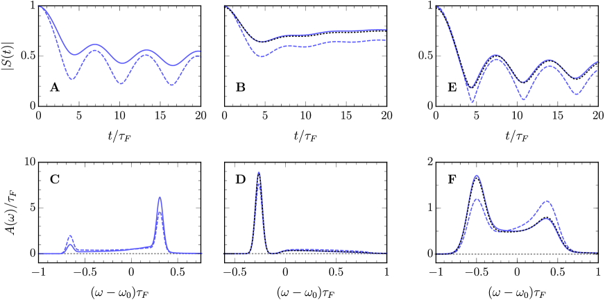
In order to analyze the role of multiple particle-hole excitations, we first consider the limit of a fixed (infinitely heavy) impurity at zero temperature. In this scenario, the FDA yields the exact solution of the impurity problem. Since, in this case, the TBM only differs from the FDA by its neglect of multiple particle-hole excitations, a comparison of the predictions of the two methods allows us to isolate the effect of these excitations.

In Fig. 5 we display the predictions for the Ramsey response using the two theoretical approaches. We find that both theoretical predictions agree extremely well at short times. In particular, for both the amplitude and phase of , our results imply that multiple particle-hole excitations start to influence our observables at a time scale of around , and only become prominent beyond . Thus, at shorter time scales, multiple particle-hole excitations can be neglected when predicting the results of the Ramsey measurements.
We note that the fixed impurity scenario is a worst-case scenario for the TBM: At , the infinitely heavy impurity is subject to the orthogonality catastrophe with an associated power-law decay of the Ramsey contrast at long times Anderson (1967). This decay, which arises due to an infinite number of particle-hole fluctuations and which leads to a vanishing quasiparticle weight, is exactly incorporated in the FDA. By contrast, in the long-time limit, the TBM predicts the saturation of to a constant value (see Fig. 5), corresponding to a spurious finite residue. However, for a mobile impurity at zero temperature, recoil becomes relevant. These recoil effects lead to the absence of the orthogonality catastrophe Rosch (1999), and thus to an increased accuracy of the TBM in the case of finite impurity mass.
Generally, one expects that the relevant time scale for multiple particle-hole excitations is closely related to the Fermi time . As discussed above, we find that such excitations become relevant for a description of only at around or beyond. This observation can be understood in a twofold way. First, in the equilibrium case it was found that contact interactions in the Fermi polaron problem lead to an approximate cancellation of terms involving identical fermions, thus suppressing the emergence of multiple particle-hole fluctuations Combescot and Giraud (2008). Our observation may hence be interpreted as a generalization of these findings to the non-equilibrium case. Second, the spectrum of the Fermi polaron problem features a dominant contribution involving the excitation of fermions from the bottom of the Fermi sea to the Fermi surface Knap et al. (2012). As discussed in Ref. Knap et al. (2012), these excitations manifest themselves as oscillations with period in the Ramsey contrast . Such a bottom of the band excitation is also present in the truncated wavefunction (8), and indeed the remarkable agreement of the TBM with the exact solution from the FDA up to the time suggests that this effect can be captured by single-particle hole excitations.
S2.2 Impurity mass

As discussed in the main text, our experimental findings are well described by the static impurity approximation, although the impurity has finite mass. To quantify the effect of the finite impurity mass, we study here the case of zero temperature. This allows us to isolate the effect of finite impurity recoil from the influence of thermal fluctuations, which will become dominant beyond times , as discussed in the section below. In order to estimate at which time scale recoil becomes important, we make use of the capability of the TBM to describe impurities of arbitrary mass. Furthermore, our analysis in Sec. S2.1 shows that the TBM yields highly accurate results for the short-time dynamics of . Accordingly, in Fig. 6 we display the Ramsey response for a static impurity and for the experimentally relevant impurity mass, both calculated within the TBM. We see that for both amplitude and phase, the impurity motion only results in a small difference in the Ramsey signal at times . Physically, this time scale corresponds to the effective recoil time associated with Li collisions on K atoms, which we estimated in Sec. S1.3 to be , in agreement with our findings here. At times exceeding , we find that the dynamics is indeed affected by the finite impurity mass. However, at such times, thermal fluctuations dominate the behavior in experiment, as we now discuss.
S2.3 Temperature
At long times, the time evolution reduces to a simple exponential decoherence of . The time scale at which this crossover to exponential decay takes place is given by the thermal time scale . In our experiment, where , this corresponds to and, hence, we observe both regimes within the dynamical range probed in our experiment.
In this section, we use finite-temperature FDA calculations to gauge the role of temperature in the impurity dynamics. To this end we compare the results for the Ramsey signal at zero and finite temperature for the experimentally realized parameters. The results are shown in Fig. 7. We indeed find that at times the time evolution at finite temperature starts to deviate from the purely quantum behavior. Finite temperature leads to an exponential decoherence of the Ramsey signal and has the consequence that thermal fluctuations dominate over the impurity motion at times Rosch (1999). Hence they mask the effect of impurity recoil as discussed in Sec. S1.3.
Overall, the conditions in our experiment give rise to three competing time scales. Multiple particle hole excitations become relevant for our measurement of at around , the recoil time is , and the thermal scale is set by . A comparison of these scales reveals the reason for the remarkable agreement between the FDA and experiment: Recoil is only weakly probed at short times , while its effect is washed out by the thermal fluctuations at long times .
S3 Role of interaction during finite-length rf pulses
In this section, we analyze the role of the ‘imperfect’ interaction quench in our experiments, where residual interactions are present during the rf pulses. Furthermore, we discuss how our findings pave the way towards the use of our experimental techniques to exert control over many-body states in real time.
S3.1 Idealized versus realized Ramsey scenario
Thus far, we have assumed the idealized scenario of a perfect two-pulse Ramsey scheme. In this case, the initial spin state of the impurity (K in the experiment) is non-interacting with the Li Fermi sea and there are no interactions during the applied rf pulses.Each pulse then yields a perfect rotation on the Bloch sphere, e.g., the initial state K is transformed into the spin-state superposition . For such a perfect Ramsey sequence, the measured Ramsey signal gives the overlap between the time-evolved interacting and non-interacting states of the system Goold et al. (2011); Knap et al. (2012), yielding Eqs. (9) and (14) for zero and finite temperature, respectively. In this idealized scenario, the Fourier transform of corresponds to the excitation spectrum of the system in linear response Mahan (1990),
| (15) |
where is the frequency of the applied field.
In our experiments, however, residual interactions are present during the pulses, which take a finite time to be completed. As shown in the illustration of our experimental sequence in Fig. 8, the state K can already interact with the Li cloud during the rotation, which potentially affects the observed dynamics of the system. Specifically, this stage of the experiment is performed at a detuning from the Feshbach resonance which corresponds to a weak interaction strength between the impurities and the Fermi sea (cf. Section S3.2 and Fig. 8). After preparing the superposition state of the impurity spin, we quench the system to strong interactions (interaction parameter ) by optically shifting the Feshbach resonance Cetina et al. (2015). We previously focussed on the complex non-equilibrium dynamics resulting from the strong interactions during the time . In the following, we analyze the effect of the residual interaction during the finite-duration spin rotations. In particular, we investigate the impact of these weak interactions during the rf pulses on the Ramsey response and the spectrum as obtained from the Fourier transform Eq. (15).
S3.2 Modelling of rf pulses within TBM
In this section, we extend our modelling of the zero-temperature impurity dynamics within the TBM to directly simulate the entire experimental procedure, as illustrated in Fig. 8. In order to model the rf pulses, we explicitly include both K and K spin states, as well as the rf field. This modifies the Hamiltonian, Eq. (1), to with the additional term
| (16) |
Here, we have used the rotating wave approximation. corresponds to the strength of the rf field, is the variable phase of the second rf pulse, and creates a particle in the state K with momentum . Note that in the original two-channel Hamiltonian (1). The interactions during the rf pulses cause a shift in the transition frequency between the K and K states from the bare transition frequency to , where is the polaron energy at interaction parameter . As described in Sec. S5.B, we account for this shift by adjusting the frequency of our rf pulses to .
According to the last term in Eq. (16), the shift in the frequency of the rf source from to causes the observed signal to accumulate an additional phase during the interaction time . To account for this, we introduce the phase . We then determine and the phase by noting that the Ramsey signal corresponds to a sine-wave function of plus an offset, i.e., it takes the form with a real, -independent function. This mirrors the experimental procedure, where , , and appear as fit-parameters for the Ramsey signal, see Sec. S5.B.
Within the TBM, we determine the approximate eigenstates and eigenvalues of within the more general class of truncated wavefunctions:
To model the experimental quench sequence illustrated in Fig. 8, we apply a series of time evolution operators to the initial state consisting of a K atom and the Li Fermi sea. At the end of the sequence we then extract the number of K atoms in states K and K, respectively. We include explicitly the rf pulses, the wait times, and the interaction time during which the system is strongly interacting. The results of this procedure are displayed in Fig. 2 of the main text. Here, we account for slight additional experimental decoherence by scaling the prediction for as described in Section S.5C.
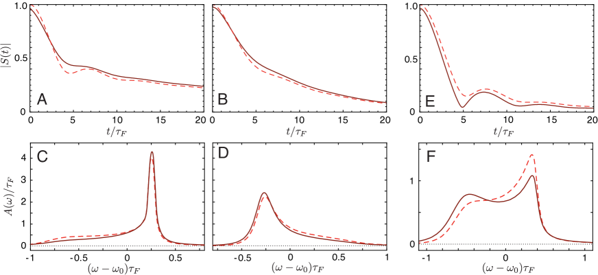
In the upper panels of Fig. 9 we compare the Ramsey response obtained by simulating the actual experimental sequence (solid line) with that of the perfect quench scenario (dashed line). We see that the residual interactions in experiment can indeed influence the quantum evolution of the impurity. The difference in the responses can be straightforwardly explained by assuming that the main effect of is to produce a weakly interacting initial state. Specifically, for weak attractive interactions , the Ramsey response can be approximated as
| (17) |
where is the ground state of the Hamiltonian (1) at interaction parameter , and is the corresponding polaron residue. Note that we cannot formally construct a similar expression for the repulsive case , since the repulsive polaron is a metastable state, involving multiple eigenstates of the Hamiltonian.
Referring to Fig. 9, the excellent agreement between the approximation (17) and the full Ramsey signal provides strong evidence that the residual interactions produce a weakly attractive initial state. This is further supported by the spectrum shown in the bottom panels, where we see that the residual interactions enhance the attractive polaron peaks for and . A similar enhancement of the repulsive polaron peak is observed for . Hence we conclude that the explicit modelling of the impurity dynamics using the full Hamiltonian is not essential for the description of the dynamics during the initial spin rotation and instead one can fully describe the time evolution using the Hamiltonian (1).
S3.3 Modelling of experimental procedure at finite temperature within FDA
The interplay between the residual interactions and finite temperature presents a further theoretical challenge. In the following, we use the FDA to simulate the experimental protocol (Fig. 8) at finite temperature. To achieve this, we exploit the finding from Sec. S3.2 that the detailed dynamics of the rf-driven oscillations between the K and K states can be ignored when calculating . Thus, we assume that the initial rotation effectively produces a spin superposition , independently of the residual interaction of the impurity in the state K with the Fermi sea. To account for the dynamics due to the weak interaction , we then let the system evolve under this interaction for a hold time , which models the dynamics at weak interaction as the result of a sudden switch-on of this interaction at the midpoint of the pulses. After the hold time , the final quench to the strong interactions is performed. For the measurement of the Ramsey contrast, this sequence is reversed. Theoretically, this yields the modified time-dependent overlap
| (18) |
where and denote the Hamiltonian (1) at interaction strength and , respectively. Using the FDA, the expression Eq. (18) is evaluated exactly according to Eq. (13) at the experimental temperature. As can be inferred from Eq. (18), this simplified model of the experimental protocol corresponds to a sequence of interaction quenches.
In the upper panel of Fig. 10 we compare the result for at the experimental temperatures obtained for the experimental sequence (solid lines) to the result for an idealized, i.e., perfect quench, Ramsey sequence (dashed lines). Similarly to the case of zero temperature, we see that the time evolution at has an experimentally observable effect on the dynamics. In particular, it generates an additional decoherence of the Ramsey signal already at , as well as an enhancement of the oscillations in for resonant interactions – see Fig. 10E.
For the calculation of the FDA results shown in Fig. 2 of the main text we use the same procedure as described above. We account for slight additional experimental decoherence by scaling the prediction for as described in Section S.5C. We also note that the phase of the Ramsey signal , as determined from Eq. (18), differs from the experimentally measured phase due to the detuning of the rf frequency from . They are related by . Similar to the previous section and to the experiment, we take .
As outlined in Section S3.1, in the idealized Ramsey scenario the Fourier transform of is equivalent to the rf absorption in linear response, cf. (15) Knap et al. (2012). Similarly to our analysis in Sec. S3.2, we now study the effect of the residual interactions on the spectral decomposition of . To this end we compare the two signals for the perfect quench with the result obtained for the experimental sequence as modelled by Eq. (18). We show the comparison of the spectra obtained in the idealized (dashed) and experimentally realized scenario (solid) in the lower panel of Fig. 10. As for our results discussed above, we find only a small difference between the two finite-temperature spectra. Therefore, in agreement with the experimental observation, cf. Fig. 3 in the main paper, under the condition of we see that the weak interactions during the rf pulses have an observable but small effect on the predicted spectra.
In accordance with the results from the TBM shown in Fig. 9, we find from the evaluation of Eq. (18) that weak interactions lead to a small shift of spectral weight into the corresponding dominant polaron branches. This shift of spectral weight is also observed experimentally, see Fig. 3 of the main text.
S3.4 Stronger interactions during rf pulses: illustration of quantum state preparation
The shift of spectral weight towards the attractive or repulsive branches of the spectrum, cf. Figs. 9 and 10, may be interpreted as follows: The residual interactions present during the initial impurity spin rotation serve to produce an interacting many-body quantum state. As such, this procedure can be viewed as an adiabatic preparation of an attractive or repulsive polaron. Compared to the noninteracting state, this polaron has an increased wavefunction overlap with the corresponding branch of the strongly interacting system. When the system is then quenched into the regime of strong interactions, the increased overlap results in the corresponding shift of the spectral weight. An intriguing question is then whether such an approach can provide a novel way to experimentally control the spectral decomposition of quantum states.
To investigate this possibility, we increase the interaction during the rotations, corresponding to decreasing , and determine the effect on . In the upper panel of Fig. 11 we show the spectra obtained by linear-response rf spectroscopy (green squares). Similar to Fig. 3 of the main paper, we compare this result to the Fourier transform of the Ramsey signal (gray shading), as obtained from the experimental sequence described in Fig. 8. We also compare our experimental result to the prediction from the FDA, where the dynamics has been modelled as described by Eq. (18). As in the main text, we find excellent agreement between experiment and theory. Indeed, both feature a strong shift of spectral weight to regions of the spectrum that are adiabatically connected to the dominant polaron branches at interaction . Furthermore, when comparing in Fig. 11, with the spectrum for in Figs. 9 and 10, it is clear that the amount by which the spectrum is shifted can be controlled by the strength of the interaction during the rf pulses. This strongly supports the assertion that the initial interactions can be used to precisely control the many-body dynamics. Our experimental techniques thus allow for a precise, dynamic control of the spectral decomposition of quantum states in future experiments.
The excellent agreement between theory and experiment also demonstrates that our theoretical approaches can be used to explore experimental ramps in combination with interferometric protocols in order to find, for instance, optimized spin and interaction trajectories.
S4 Universal features of impurity dynamics and relation to orthogonality catastrophe
For impurities localized in space, which, for instance, can be achieved by species-selective three dimensional optical lattices, our experimental setup allows one to study universal features exhibited by the Anderson orthogonality catastrophe Anderson (1967). The orthogonality catastrophe was originally studied in the context of x-ray absorption spectra in metals, where high-energy x-ray photons create atomic core holes by photoemission of inner-shell electrons Mahan (1990). These core holes produce a scattering potential for the electrons in the conduction band, leading to characteristic power-law edges in the absorption spectra with an exponent that is universally determined by the scattering phase shift at the Fermi surface Anderson (1967). However, impurities, phonons, residual interactions between the electrons, and a lack of knowledge of microscopic parameters makes it difficult to unambiguously determine the universal features of the orthogonality catastrophe in typical solid state materials Ohtaka and Tanabe (1990). In contrast, the Hamiltonian in our experiment is well characterized on all relevant energy scales, and therefore the full dynamic response of the system can be reliably calculated by theory and probed by the ultrafast experimental techniques demonstrated in this work. This enables one to obtain fundamental insights into universal features of the orthogonality catastrophe, which are difficult to access in other systems.
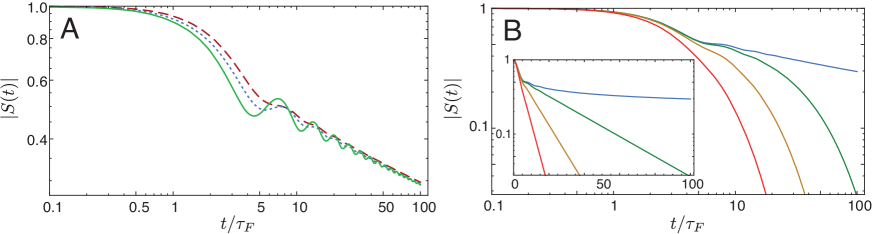
To illustrate how the orthogonality catastrophe would manifest itself in an ultracold atomic gas experiment, the response of infinite mass impurities calculated using the FDA for the perfect quench scenario is shown in Fig. 12. First, at short times and for a range parameter of the Feshbach resonance , we see that the Ramsey contrast decays quadratically for all scattering parameters and temperatures considered, in accordance with Eq. (11). The main universal feature associated with the orthogonality catastrophe is expected in the long-time dynamics at : Here, the Ramsey response is predicted to exhibit power law tails, which depend only on the scattering phase shift at the Fermi surface Anderson (1967); Knap et al. (2012). This is explicitly verified in Fig. 12A where we fix the scattering phase shift at the Fermi surface but change the scattering parameters. While the response at intermediate times depends on the scattering parameters, we see that the long-time evolution approaches a universal power law that only depends on the phase shift at the Fermi surface. We note that the long-time dynamics is universal: It is the same for a system with a broad resonance where (solid line in Fig. 12A), as it is for our system with a finite range parameter (dashed and dotted lines).
When the temperature is non-zero, as in the experiment, thermal fluctuations alter the power law dephasing dynamics at sufficiently long times. Instead, exponential tails due to thermal decoherence appear as another universal feature of the dynamics Korringa (1950); Anderson (1967); Yuval and Anderson (1970); Knap et al. (2012). The exponential tails are illustrated in Fig. 12B. The effects of thermal decoherence could be countered by employing the recently developed cooling methods Hart et al. (2015), opening the door to observing the orthogonality catastrophe in a cold-atom system.
Finally, we note that in our experiment temperature becomes relevant at a time scale similar to those associated with recoil and multiple particle-hole excitations. It is a challenge for theoretical approaches to exactly account for both recoil and higher order particle-hole excitations Rosch (1999). However, experiments at lower temperatures which take advantage of the tunability of the impurity mass using optical lattices would be ideally suited to probe the competition between these effects. Such ultracold-atom experiments would hence provide important insight into this long standing theoretical question.
S5 Experimental and data analysis procedures
In this section we discuss the procedures used to record and analyze the data presented in this work. We detail the cooling and preparation of our atomic samples, the details of the rf pulses used in our Ramsey sequences, the methods used to analyze the data and the method that we use to vary the concentration of the K atoms.
S5.1 Sample preparation
The atomic samples are prepared by forced evaporation of Li atoms from a Li-K mixture held in an optical trap, where the K atoms are sympathetically cooled by the Li environment. This preparation procedure is described in detail in Refs. Trenkwalder et al. (2011); Spiegelhalder et al. (2010). At the end of the forced evaporation, the Li and K atoms are transferred into an optical trap composed of two crossed 1064-nm laser beams, as described in Ref. Cetina et al. (2015). The measured radial and axial trap frequencies of the Li atoms are Hz and Hz, respectively. The measured radial and axial trap frequencies of the K atoms are Hz and Hz, respectively.
At the end of the preparation procedure, the Li and the K atoms are in their lowest Zeeman states Li and K. Before the Ramsey sequence, the K atoms are transferred to the K state using an rf pulse. Following this rf transfer, the Li and K atoms are thermalized by holding them for 750 ms in the crossed-beam optical trap. While the interaction between the Li and K atoms, characterized by the scattering length Naik et al. (2011), is sufficient to ensure thermalization during this hold time, it can be neglected during the Ramsey experiments. The temperature of the atoms is determined by releasing the atoms from the trap and observing the free expansion of the K cloud.
Due to the Li Fermi pressure and the more than two times stronger optical potential for K, the K cloud is much smaller than the Li cloud Trenkwalder et al. (2011), and therefore samples a nearly homogeneous Li environment. Because of the small variation of the Li environment sampled by the K atoms, we introduce the effective Li Fermi energy as
| (19) |
Here, is the local K number density at position in the trap, and
| (20) |
is the local Li Fermi energy as determined by the local Li number density . We quantify the small inhomogeneity of the Li environment experienced by the K atoms by the standard deviation of the local Li Fermi energy
| (21) |
We also introduce the average Li and K number densities and sampled by the K atoms as
| (22) |
In contrast to the Li atoms, the K atoms in our measurements remain non-degenerate, with , where is the local potassium Fermi energy in the center of the trap when all K atoms are in the same internal state.
| Figure(s) | |||||||
|---|---|---|---|---|---|---|---|
| (nK) | (kHz) | % | cm-3 | cm-3 | |||
| 2A, 2C, 3A | 3.5(4) | 0.95(10) | 435(25) | 7.4 | 8.9(7) | 1.8(3) | |
| 2B, 2D, 3B | 3.3(4) | 1.0(1) | 410(25) | 7.1 | 8.7(6) | 2.0(3) | |
| 2E, 2F, 3C | 3.5(4) | 1.0(1) | 460(30) | 7.7 | 8.8(6) | 1.7(3) | |
| 11A | 3.1(4) | 1.0(1) | 430(30) | 7.7 | 8.2(7) | 1.8(3) | |
| 11B | 2.9(3) | 1.05(10) | 425(35) | 7.7 | 8.0(6) | 2.0(3) | |
| 4 | 2.35(30) | 2.5(1) | 520(25) | 10.4 | 6.5(5) | 3.4(3) |
For all measurement presented in this work, Table 1 lists the total numbers of the Li and K atoms, their temperatures and trap-averaged densities, as well as the effective Li Fermi energies and their standard deviations. Throughout our measurements, these parameters remain nearly constant, with the exception of the measurements shown in Fig. 4. Here, in order to investigate the effect of the K concentration, the total number of the K atoms is increased from about to . The attendant increase in the thermal load during the Li evaporation results in a decrease of the Li atom number and an increase in the temperature of the final atomic sample.
Note that, in contrast to our previous work Cetina et al. (2015), our present experiments have been optimized for large optically induced interaction shifts (). These shifts are produced by switching one of the crossed trapping beams from a beam with a low peak intensity and small size to a beam with a large intensity and large size propagating in the same direction. In our previous work Cetina et al. (2015), as well as in the measurements shown in Fig. 11, the waists, positions and intensities of the two beams are adjusted so as to yield mode-matched trapping potentials, preventing excitations of the center-of-mass and breathing collective modes of the atomic clouds. In the measurements presented in Figs. 2, 3 and 4, a larger beam intensity was used in order to produce a larger optical shift, resulting in some excitation of the breathing modes.
The maximal interaction time in our Ramsey measurements of 60 s is much smaller than the shortest period of a collective oscillation (about 500 s). We calculate that, during our short interaction time, the oscillations of the breathing modes cause at most a 6% variation of around its initial value specified in Table 1, without any significant effect on the measurements presented here.
S5.2 Rf pulses
We apply rf pulses in the Ramsey procedures by discretely gating a continously running rf source. To record the atomic populations and as a function of the phase of the second rf pulse, we change the phase of the rf source by a variable amount before applying this pulse.
The weak interactions between the K atoms in the K state and the Li atoms corresponding to the interaction parameter cause the transition frequency between the K and the K states to differ from the transition frequency in the absence of the Li atoms. We compensate for this effect by adjusting the frequency of the rf source to be resonant with the KK transition at the time when the rf pulses are applied. For the data in Figs. 2A, 2B, 2C, is equal to , , , respectively. For the data in Fig. 11C and 11D where the interaction of the K atoms during the rf pulses is stronger, is equal to and .
The shift in the frequency of the rf source from to causes the signal to accumulate an additional phase during the interaction time . To account for this added phase, we introduce the phase .
S5.3 Analysis methods
We determine the contrast and the phase by fitting the Ramsey signal as a function of the phase to a sine wave with an offset i.e. . Decoherence during the rf pulses, as well as imperfections of the rf pulses and the atom detection, cause the contrast for to be slightly smaller than unity. When comparing theoretical results from Figs. 9 and 10 to the experimental data in Fig. 2, we account for this effect by scaling the theoretical predictions for by an overall factor . For each calculation, this factor is determined by fitting the prediction for to the three data points with the the shortest interaction times. We obtain , which corresponds to an additional loss of contrast that is of the same order as the decoherence during the rf pulses predicted by the FDA (see Fig. 10).
To compute the Fourier transform of the experimental data, we use piecewise linear interpolations of and between the individual data points. Outside of the range of the data, we set . To determine the error of the Fourier transform, we sample the values of and at each data point from Gaussian distributions whose means and standard deviations correspond to the measured values and errors, respectively. We use the standard deviation of the computed values of the Fourier transform for each value of as an estimate of the error indicated by the shaded areas in Figs. 3 and 11.
S5.4 Varying the K concentration
We study the effects of the impurity concentration by varying the number of the strongly interacting K atoms. If this were done by changing the total number of the K atoms in the experiment, the change in the thermal load on the Li atoms during forced evaporation would result in a correlated variation in the number of Li atoms and the sample temperature (compare the settings for Fig. 2 and Fig. 4 in Table 1). To avoid these systematic effects, in the measurements presented in Fig. 4, we keep the total number of the K atoms constant and vary the fraction of the K atoms that participate in the Ramsey sequence. We accomplish this by changing the intensity of the rf pulse that transfers the K atoms from the state to the state before the Ramsey procedure. During the subsequent 750 ms preceding the Ramsey sequence, the K atoms collisionally thermalize with the much larger Li cloud, resulting in an incoherent mixture of K and K atoms at a constant temperature. When referring to these measurements, we use not for the average density of all K atoms, but for the density of those K atoms that participate in the Ramsey sequence.
We minimized the small effects of long-time drifts in the temperature, the atom numbers and the trapping potential by varying the experimental parameters in a specific order. For each K concentration and interaction time, we recorded data for 4 different phases of the second rf pulse in order to obtain . For each interaction time, the data with different K concentrations were recorded in immediate succession. The data sets for different interaction times were then recorded in a random order.
S6 Linearity of rf response
The response of atoms to an applied rf field is linear if the fraction of the atoms transferred from one state to another is proportional to the intensity of the field. Linearity can be ensured by using a sufficiently weak rf pulse that is also much longer than the inverse width of the relevant spectral features. The narrowest spectral features in the present work are the polaron peaks in Figs. 3A and 3B with rms widths and , respectively. To record these polaron spectra, we used Blackman-shaped rf pulses Kasevich and Chu (1992) whose duration is much longer than the inverse widths of the polaron peaks.
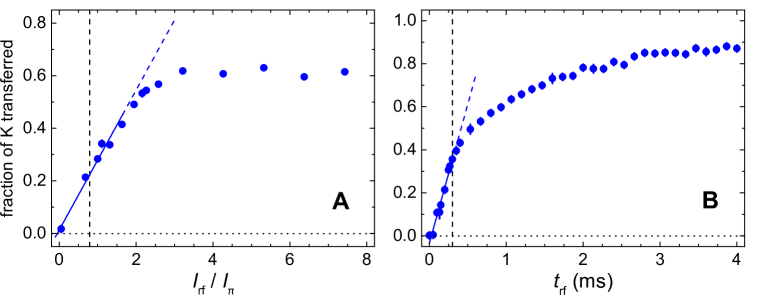
We checked the linearity of the response by varying the intensity of the applied rf field. Fig. 13A shows the fraction of the K atoms transferred from the K to the K state in the repulsive polaron regime, under conditions similar to those in the measurements shown in Fig. 3A. The frequency of the rf pulse is adjusted so that , corresponding to peak response and resonant excitation of the repulsive polaron. The rf intensity is measured in units of the intensity that results in a -pulse for noninteracting K atoms. For intensities up to the intensity , which is used in the measurements shown in Figs. 3A and 3B, we observe that the transferred fraction of the K atoms stays essentially proportional to the intensity of the pulse.
In the linear-response regime, the atomic response is predicted to be proportional to the duration of the rf pulse. Fig. 13B shows the fraction of the K atoms transferred in the repulsive polaron regime by rf pulses with , as a function of the pulse duration. The frequency of the rf pulse is adjusted so that , in order to obtain the peak response, as in Fig 13A. For pulses with duration up to 300 s (indicated by the dashed line), we observe that the transferred fraction of the K atoms stays essentially proportional to the duration of the pulse.
Note that the maximal transferred fraction exceeds 0.5. We explain this observation by the coupling of the initial non-interacting K state to multiple interacting K states by the rf pulse, which manifest themselves as the polaron peak and the broad pedestal in our spectra.
The spectra for resonant Li-K interactions shown in Figs. 3B, 11A, 11B were recorded using Blackman-shaped rf pulses with duration of s (approximately ). The intensity of these pulses was adjusted to 50% of that needed to produce pulses for noninteracting K atoms. We verified the linearity of the rf response by comparing the spectra recorded using this rf intensity to those recorded using the intensity needed to produce full pulses for noninteracting K atoms (Fig. 14). Our observations are in good agreement with linear response.
References
- Krausz and Ivanov (2009) F. Krausz and M. Ivanov, Rev. Mod. Phys. 81, 163 (2009).
- Pazourek et al. (2015) R. Pazourek, S. Nagele, and J. Burgdörfer, Rev. Mod. Phys. 87, 765 (2015).
- Cronin et al. (2009) A. D. Cronin, J. Schmiedmayer, and D. E. Pritchard, Rev. Mod. Phys. 81, 1051 (2009).
- Simon et al. (2011) J. Simon, W. S. Bakr, R. Ma, M. E. Tai, P. M. Preiss, and M. Greiner, Nature (London) 472, 307 (2011).
- Atala et al. (2013) M. Atala, M. Aidelsburger, J. T. Barreiro, D. Abanin, T. Kitagawa, E. Demmler, and I. Bloch, Nature Physics 9, 795 (2013).
- Gring et al. (2012) M. Gring, M. Kuhnert, T. Langen, T. Kitagawa, B. Rauer, M. Schreitl, I. Mazets, D. A. Smith, E. Demler, and J. Schmiedmayer, Science 337, 1318 (2012).
- Hadzibabic et al. (2006) Z. Hadzibabic, P. Krüger, M. Cheneau, B. Battelier, and J. Dalibard, Nature (London) 441, 1118 (2006).
- Koschorreck et al. (2013) M. Koschorreck, D. Pertot, E. Vogt, and M. Kohl, Nat. Phys. 9, 405 (2013).
- Bardon et al. (2014) A. B. Bardon, S. Beattie, C. Luciuk, W. Cairncross, D. Fine, N. S. Cheng, G. J. A. Edge, E. Taylor, S. Zhang, S. Trotzky, et al., Science 344, 722 (2014).
- Goold et al. (2011) J. Goold, T. Fogarty, N. Lo Gullo, M. Paternostro, and T. Busch, Phys. Rev. A 85, 063632 (2011).
- Knap et al. (2012) M. Knap, A. Shashi, Y. Nishida, A. Imambekov, D. A. Abanin, and E. Demler, Phys. Rev. X 2, 041020 (2012).
- Cetina et al. (2015) M. Cetina, M. Jag, R. S. Lous, J. T. M. Walraven, R. Grimm, R. S. Christensen, and G. M. Bruun, Phys. Rev. Lett. 115, 135302 (2015).
- (13) See supplementary materials.
- Naik et al. (2011) D. Naik, A. Trenkwalder, C. Kohstall, F. M. Spiegelhalder, M. Zaccanti, G. Hendl, F. Schreck, R. Grimm, T. Hanna, and P. Julienne, Eur. Phys. J. D 65, 55 (2011).
- Loschmidt (1876) J. Loschmidt, Sitzungsberichte der Akademie der Wissenschaften, Wien 73, 128 (1876).
- Jalabert and Pastawski (2001) R. A. Jalabert and H. M. Pastawski, Advances in Solid State Physics 41, 483 (2001).
- Massignan et al. (2014) P. Massignan, M. Zaccanti, and G. M. Bruun, Rep. Prog. Phys. 77, 034401 (2014).
- Chevy (2006) F. Chevy, Phys. Rev. A 74, 063628 (2006).
- Nozières and de Dominicis (1969) P. Nozières and C. T. de Dominicis, Phys. Rev. 178, 1097 (1969).
- Kohstall et al. (2012) C. Kohstall, M. Zaccanti, M. Jag, A. Trenkwalder, P. Massignan, G. M. Bruun, F. Schreck, and R. Grimm, Nature (London) 485, 615 (2012).
- Dubois et al. (2013) J. Dubois, T. Jullien, F. Portier, P. Roche, A. Cavanna, Y. Jin, W. Wegscheider, P. Roulleau, and D. C. Glattli, Nature (London) 502, 659 (2013).
- Mora and Chevy (2010) C. Mora and F. Chevy, Phys. Rev. Lett. 104, 230402 (2010).
- Yu et al. (2010) Z. Yu, S. Zöllner, and C. J. Pethick, Phys. Rev. Lett. 105, 188901 (2010).
- Zwerger (2012) W. Zwerger, ed., The BCS-BEC Crossover and the Unitary Fermi Gas (Springer, Berlin, 2012).
- Hart et al. (2015) R. A. Hart, P. M. Duarte, T.-L. Yang, X. Liu, T. Paiva, E. Khatami, R. T. Scalettar, N. Trivedi, D. A. Huse, and R. G. Hulet, Nature (London) 519, 211 (2015).
- LeBlanc and Thywissen (2007) L. J. LeBlanc and J. H. Thywissen, Phys. Rev. A 75, 053612 (2007).
- Chin et al. (2010) C. Chin, R. Grimm, P. S. Julienne, and E. Tiesinga, Rev. Mod. Phys. 82, 1225 (2010).
- Schmidt et al. (2012) R. Schmidt, S. Rath, and W. Zwerger, Eur. Phys. J. B 85, 1 (2012).
- Bruun and Pethick (2004) G. M. Bruun and C. J. Pethick, Phys. Rev. Lett. 92, 140404 (2004).
- Petrov (2004) D. S. Petrov, Phys. Rev. Lett. 93, 143201 (2004).
- Góral et al. (2004) K. Góral, T. Köhler, S. A. Gardiner, E. Tiesinga, and P. S. Julienne, J. Phys. B 37, 3457 (2004).
- Szymańska et al. (2005) M. H. Szymańska, K. Góral, T. Köhler, and K. Burnett, Phys. Rev. A 72, 013610 (2005).
- Parish and Levinsen (2013) M. M. Parish and J. Levinsen, Phys. Rev. A 87, 033616 (2013).
- Vlietinck et al. (2013) J. Vlietinck, J. Ryckebusch, and K. Van Houcke, Phys. Rev. B 87, 115133 (2013).
- Levitov et al. (1996) L. S. Levitov, H. Lee, and G. B. Lesovik, J. Math. Phys. 37, 4845 (1996).
- Levitov and Lesovik (1993) L. Levitov and G. Lesovik, JETP Lett. 58, 230 (1993).
- Klich (2003) I. Klich (Kluwer, Dordrecht, 2003), pp. 397–402.
- Rosch (1999) A. Rosch, Adv. Phys. 48, 295 (1999).
- Anderson (1967) P. W. Anderson, Phys. Rev. Lett. 18, 1049 (1967).
- Combescot and Giraud (2008) R. Combescot and S. Giraud, Phys. Rev. Lett. 101, 050404 (2008).
- Mahan (1990) G. D. Mahan, Many-particle physics, Physics of solids and liquids (Plenum, New York, NY, 1990).
- Ohtaka and Tanabe (1990) K. Ohtaka and Y. Tanabe, Rev. Mod. Phys. 62, 929 (1990).
- Korringa (1950) J. Korringa, Physica 16, 601 (1950).
- Yuval and Anderson (1970) G. Yuval and P. Anderson, Phys. Rev. B 1, 1522 (1970).
- Trenkwalder et al. (2011) A. Trenkwalder, C. Kohstall, M. Zaccanti, D. Naik, A. I. Sidorov, F. Schreck, and R. Grimm, Phys. Rev. Lett. 106, 115304 (2011).
- Spiegelhalder et al. (2010) F. M. Spiegelhalder, A. Trenkwalder, D. Naik, G. Kerner, E. Wille, G. Hendl, F. Schreck, and R. Grimm, Phys. Rev. A 81, 043637 (2010).
- Kasevich and Chu (1992) M. Kasevich and S. Chu, Phys. Rev. Lett. 69, 1741 (1992).