Learning Arbitrary Sum-Product Network Leaves with Expectation-Maximization

Abstract

Sum-Product Networks with complex probability distribution at the leaves have been shown to be powerful tractable-inference probabilistic models. However, while learning the internal parameters has been amply studied, learning complex leaf distribution is an open problem with only few results available in special cases. In this paper we derive an efficient method to learn a very large class of leaf distributions with Expectation-Maximization. The EM updates have the form of simple weighted maximum likelihood problems, allowing to use any distribution that can be learned with maximum likelihood, even approximately. The algorithm has cost linear in the model size and converges even if only partial optimizations are performed. We demonstrate this approach with experiments on twenty real-life datasets for density estimation, using tree graphical models as leaves. Our model outperforms state-of-the-art methods for parameter learning despite using SPNs with much fewer parameters.

1 Introduction

Sum-Product Networks (SPNs, [Poon and Domingos, 2011]) are recently introduced probabilistic models that possess two crucial characteristics: firstly, inference in a SPN is always tractable; secondly, SPN enable to model tractably a larger class of distributions than for Graphical Models because they can model efficiently context specific dependences and determinism ([Boutilier et al., 1996]). Due to their ability to use exact inference in complex distributions SPNs are state-of-the-art models in density estimation (see e.g. [Gens and Domingos, 2013, Rahman and Gogate, 2016b]) and have been successfully used in computer vision ([Cheng et al., 2014], [Peharz et al., 2014], [Amer and Todorovic., 2015]).

SPNs are modelled by a directed acyclic graph with two sets of parameters: edge coefficients at internal sum nodes and probabilistic distributions at the leaves. Most SPN models use very simple leaf models in form of indicator variables. However, using leaf distributions with complex structure allows to create SPNs with high modelling power and flexibility, as shown for instance in [Rahman and Gogate, 2016a] using tree graphical models as leaves and in [Amer and Todorovic., 2015] using Bag-of-Words (example: fig. 1). While there are several methods to learn edge coefficients ([Gens and Domingos, 2012, Zhao et al., 2016b, Zhao et al., 2016a]), learning the leaf distribution parameters is still an open problem in the general case. The only method we are aware of is [Peharz et al., 2016], which works for the special case of univariate distribution in the exponential family (although the authors suggest it can be extended to the multivariate case).

The goal of this paper is to learn leaf distributions with complex structure in a principled way. To do so, we obtain a novel derivation of Expectation-Maximization for SPNs that allows to cover leaf distribution updates (section 4). The first step in this derivation is providing a new theoretical result relating the SPN and a subset of its encoded mixture (Proposition 2 in the following). Exploiting this new result EM for SPN leaves assumes the form of a weighted maximum likelihood problem, which is a slight modification of standard maximum likelihood and is well studied for a wide class of distributions. The algorithm has computational cost linear in the number of SPN edges.

Convergence of the algorithm is guaranteed as long as the maximization is even partially performed. Therefore, any distribution where at least an approximate log-likelihood maximization method is available can be used as SPN leaf. This result allows to use a very wide family of leaf distributions and train them efficiently and straightforwardly. Particularly nice results hold when leaves belong to the exponential family, where the M-step has a single optimum and the maximization can often be performed efficiently in closed form.

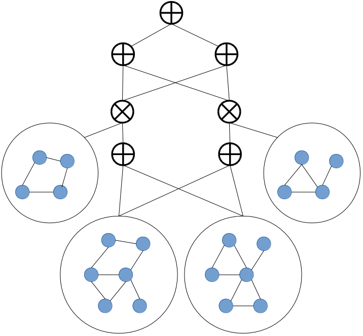
Figure 1: An example SPN with complex leaf distributions (in this case, probabilistic graphical models).

To test the potential advantages of training complex leaves we perform experiments on a set of twenty widely used datasets for density estimation, using a SPN with tree graphical models as leaf distributions (section 6). We show that a simple SPN with tree graphical model leaves learned with EM state-of-the-art methods for parameter learning while using much smaller models. These results suggests that much of the complexity of the SPN structure can be encoded in complex, trainable leaves rather than in a large number of edges, which is a promising direction for future research.

2 Sum-Product Networks

We start with the definition of SPN based on [Gens and Domingos, 2013]. Let $X$ be a set of random variables, either continuous or discrete.

Definition 1.

Sum-Product Network (SPN) :

1. A tractable distribution $\varphi(X)$ is a SPN $S(X)$.

2. The product $\prod_{k}S_{k}(X_{k})$ of SPNs $S_{k}(X_{k})$ is a SPN $S\left(\bigcup_{k}X_{k}\right)$ if all sets $X_{k}$ are disjoint.

3. The weighted sum $\sum_{k}w_{k}S_{k}(X)$ of SPNs $S_{k}(X)$ is a SPN $S(X)$ if the weights $w_{k}\in\mathbb{R}$ are nonnegative (notice that $X$ is in common for each SPN $S_{k}$).

By associating a node to each product, sum and tractable distribution and adding edges between an operator and its inputs, a SPN can be represented as a rooted Directed Acyclic Graph (DAG) $\mathcal{G}(\mathcal{V},\mathcal{E})$ with sums and products as internal nodes and tractable distributions as leaves (example: fig. 2). This definition generalizes SPNs with indicator variables as leaves, since indicator variables are a special case of discrete distribution where the probability mass completely lies on a single variable state. A SPN is normalized if weights of outgoing edges of sum nodes sum to $1$: $\sum_{k}w_{k}=1$. We consider only normalized SPNs, without loss of generality ([Peharz, 2015]).

Notation. We use the following notation throughout the paper. Let $X$ be a set of variables (either continuous or discrete depending on the context) and let $x$ be an assignment of these variables. $S_{q}\left(X_{q}\right)$ denotes the sub-SPN rooted at a node $q$ of $S$, with $X_{q}\subseteq X$. $S\left(x\right)$ denotes the evaluation of $S$ with assignment $x$ (see below), and $\frac{\partial S\left(x\right)}{\partial S_{q}}$ is the derivative of $S(x)$ w.r.t. node $q$. The term $\varphi_{l}\left(X_{l}\right)$ denotes the distribution of leaf node $l$. $ch(q)$ and $pa(q)$ denote the children and parents of $q$ respectively, and $(q,i)$ indicates an edge between $q$ and its child $i$, associated to a weight $w_{i}^{q}$ if $q$ is a sum node. Finally, let $\mathcal{E}(S)$, $\mathcal{V}(S)$ and $\mathcal{\mathcal{L}}\left(S\right)$ denote respectively the set of edges, nodes and leaves in $S$.

Parameters. Let $W$ denote the set of sum node weights and let $\theta$ denote the set of parameters governing the leaf distributions. We write $S\left(X|W,\theta\right)$ to explicitly express dependency of $S$ on these parameters. Each leaf distribution $\varphi_{l}$ is associated to a parameter set $\theta_{l}\subseteq\theta$. For instance, $\theta_{l}$ contains mean and covariance for Gaussian leaves, and tree structure and potentials for tree graphical model leaves.

Evaluation. The evaluation of $S(X)$ for evidence $x$, written $S(x)$, proceeds by first evaluating the leaf distributions with assignment $x$, then evaluating each internal node from the leaves to root and taking the value of the root. Evaluating any valid SPN corresponds to evaluating a probability distribution ([Poon and Domingos, 2011]). Computing $S(x)$, the partition function and the quantities $S_{q}\left(x\right)$ and $\frac{\partial S\left(x\right)}{\partial S_{q}}$ for each node in $S$ requires performing a single up-and-down pass over all network nodes and has a $O\left(|\mathcal{E}|\right)$ time and memory cost ([Poon and Domingos, 2011]).

3 SPNs as Mixture Models

This section discusses the interpretation of SPNs as a mixture model derived in [Dennis and Ventura, 2015] and [Zhao et al., 2016b], on which we will base our derivation of EM.

Definition 2.

A subnetwork $\sigma_{c}$ of $S$ is a SPN constructed by first including the root of $S$ in $\sigma_{c}$, then processing each node $q$ included in $\sigma_{c}$ as follows:

1. If $q$ is a sum node, include in $\sigma_{c}$ one child $i\in ch\left(q\right)$ with relative weight $w_{i}^{q}$. Process the included child.

2. If $q$ is a product node, include in $\sigma_{c}$ all the children $ch\left(q\right)$. Process the included children.

3. If $q$ is a leaf node, do nothing.

Example: fig. 2. Any subnetwork is a tree . Let $C={\sigma_{1},\sigma_{2},...,\sigma_{C}}$ be the number of different subnetworks obtainable from $S$ for different choices of included sum node children. The number of subnetworks $C$ can be exponentially larger than the number of edges $|\mathcal{E}|$.

Definition 3.

For a subnetwork $\sigma_{c}$ of $S\left(X|W,\theta\right)$ we define a mixture coefficient $\lambda_{c}=\prod_{\left(q,j\right)\in\mathcal{\mathcal{E}}\left(\sigma_{c}\right)}w_{j}^{q}$ and a mixture component $P_{c}(X|\theta)=\prod_{l\in\mathcal{L}\left(\sigma_{c}\right)}\varphi_{l}\left(X_{l}|\theta_{l}\right)$.

Note that mixture coefficients are products of sum weights and mixture components are products of leaves in $\sigma_{c}$ (fig. 2).

Proposition 1.

$S|W,\theta\left(X\right)$ represents the following mixture model:

$$S\left(X|W,\theta\right)=\sum_{c=1}^{C}\lambda_{c}\left(W\right)P_{c}\left(X|\theta\right)$$ (1)

Proof: see [Dennis and Ventura, 2015]. Notice that since $C\gg|\mathcal{E}|$, it follows that a SPN encodes a mixture which can be intractably large if explicitly represented.

Figure 2: A SPN $S\left(A,B\right)$ in which a subnetwork $\sigma_{c}$ of $S$ is highlighted. This subnetwork corresponds to a coefficient $\lambda_{c}=w_{2}^{1}w_{9}^{4}$ and component $P_{c}\left(A,B\right)=\varphi_{7}\left(B\right)\varphi_{9}\left(A\right)$.

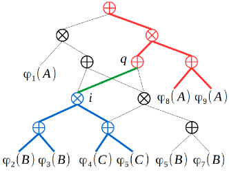
Figure 3: Visualization of Proposition 2. The colored part is the set of edges traversed by all subnetworks crossing $\left(q,i\right)$. The blue part represents $S_{i}$ and the red part $\frac{\partial S\left(X\right)}{\partial S_{q}}$.

We now introduce a new result that is crucial for our derivation of EM, reporting it here rather than in the proofs section since it contributes to the set of analytical tools for SPNs.

Proposition 2.

Consider a SPN $S(X)$, a sum node $q\in S$ and a node $i\in ch(q)$. The following relation holds:

$$\sum_{k:\left(q,i\right)\in\mathcal{E}\left(\sigma_{k}\right)}\lambda_{k}P_{k}\left(X\right)=w_{i}^{q}\frac{\partial S\left(X\right)}{\partial S_{q}}S_{i}\left(X\right)$$ (2)

where $\sum_{k:\left(q,i\right)\in\mathcal{E}\left(\sigma_{k}\right)}$ denotes the sum over all the subnetworks $\sigma_{k}$ of $S$ that include the edge $\left(q,i\right)$.

Proof: in Appendix A.1. This result states that the value of each sub-mixture composed by all the subnetworks crossing $\left(q,i\right)$, which has potentially intractable large size, can be evaluated in constant time after having evaluated and derivated $S(x)$ once. This results is crucial in the derivation of EM (Appendix A) where we need to evaluate such subsets of solutions repeatedly. Note also that $\sum_{k:\left(q,i\right)\in\mathcal{E}\left(\sigma_{k}\right)}\lambda_{k}P_{k}\left(X\right)$ corresponds to the evaluation of a non-normalized SPN which is a subset of $S$ - e.g. the colored part in fig. 3.

4 Expectation Maximization

In this section we obtain a novel derivation of Expectation-Maximization for SPNs by directly applying EM for mixture models to the exponentially large mixture encoded by a SPNs exploiting Proposition 2. We obtain a procedure to learn SPNs with a broad class of leaf distributions, and show that the algorithm converges under mild conditions.

Expectation Maximization is an elegant and widely used method for finding maximum likelihood solutions for models with latent variables (see e.g. [Murphy, 2012, 11.4]). Given a distribution $P(X)=\sum_{c=1}^{C}P\left(X,c|\pi\right)$ where $c$ are latent variables and $\pi$ are the distribution parameters our objective is to maximize the log likelihood $\sum_{n=1}^{N}\ln\sum_{c=1}^{C}P(x_{n},c|\pi)$ over a dataset of observations $\left\{x_{1},x_{2},...,x_{N}\right\}$. EM proceeds by updating the parameters iteratively starting from some initial configuration $\pi_{old}$. An update step consists in finding $\pi^{*}=\arg\max_{\pi}Q\left(\pi|\pi_{old}\right)$, where

$$Q\left(\pi|\pi_{old}\right)=\sum_{n=1}^{N}\sum_{c=1}^{C}P\left(c|x_{n},\pi_{old}\right)\ln P\left(c,x_{n}|\pi\right).$$

We want to apply EM to the mixture encoded by a SPN, which is in principle intractably large. First, using the relation between SPN and encoded mixture model in Proposition 1 we identify

$$P(c,x_{n}|\pi) =\lambda_{c}\left(W\right)P_{c}\left(x_{n}|\theta\right),$$

$$P(x_{n}|\pi_{old}) =S\left(x_{n}|W_{old},\theta_{old}\right),$$

therefore:

$$P(c|x_{n},\pi_{old})=P(c,x_{n}|\pi_{old})/P(x_{n}|\pi_{old})=\lambda_{c}\left(W_{old}\right)P_{c}\left(x_{n}|\theta_{old}\right)/S\left(x_{n}|W_{old},\theta_{old}\right).$$

Applying these substitutions and dropping the dependency on $W_{old},\theta_{old}$ for compactness, $Q\left(W,\theta|W_{old},\theta_{old}\right)$ becomes:

$$Q\left(W,\theta\right)=\sum_{n=1}^{N}\sum_{c=1}^{C}\frac{\lambda_{c}P_{c}\left(x_{n}\right)}{S\left(x_{n}\right)}\ln\lambda_{c}\left(W\right)P_{c}\left(x_{n}|\theta\right)$$ (3)

which we maximize for $W$ and $\theta$ in the following sections.

4.1 Edge Weights Update

We begin with EM updates for weights. Simplifying $Q\left(W,\theta\right)$ through the use of Proposition 2 (Appendix A.2) the objective function for $W$ becomes:

$$W^{*} =\arg\max_{W}Q_{W}\left(W\right)$$ (4)

$$Q_{W}\left(W\right) =\sum_{q\in\mathcal{N}\left(S\right)}\sum_{i\in ch\left(q\right)}\beta_{i}^{q}\ln w_{i}^{q}$$ (5)

$$\beta_{i}^{q} =w_{i,old}^{q}\sum_{n=1}^{N}S\left(x_{n}\right)^{-1}\frac{\partial S\left(x_{n}\right)}{\partial S_{q}}S_{i}\left(x_{n}\right)$$

The evaluation of terms $\beta_{i}^{q}$, which depend only on $W_{old},\theta_{old}$ and are therefore constants in the optimization, is the E step of the EM algorithm. We now maximize $Q_{W}\left(W\right)$ subject to $\sum_{i}w_{i}^{q}=1\forall q\in\mathcal{N}\left(S\right)$ (M step).

Non shared weights. If weights at each node $q$ are disjoint, then we can move the $\max$ inside the sum, obtaining separated maximizations each in the form $\arg\max_{w^{q}}\sum_{i\in ch(q)}\beta_{i}^{q}\ln w_{i}^{q}$, where $w^{q}$ is the set of weights outgoing from $q$. Now, the same maximum is attained multiplying by $k=\frac{1}{\sum_{i}\beta_{i}^{q}}$. Then, defining $\bar{\beta}_{i}^{q}=k\beta_{i}^{q}$ , we can equivalently find $\arg\max_{w^{q}}\sum_{i\in ch(q)}\bar{\beta}_{i}^{q}\ln w_{i}^{q}$, where $\bar{\beta}_{i}^{q}$ is positive and sums to $1$ and therefore can be interpreted as a discrete distribution. This is then the maximum of the cross entropy $\arg\max_{w^{q}}\left(-\mathbb{H}\left(\bar{\beta}_{i}^{q},w_{i}^{q}\right)\right)$ defined e.g. in [Murphy, 2012, 2.8.2], attained for $w_{i}^{q}=\bar{\beta}_{i}^{q}$, which corresponds to the following update:

$$w_{j}^{q*}=\beta_{j}^{q}/\sum_{i}\beta_{i}^{q}.$$ (6)

This is the same weight update obtained with radically different approaches in [Peharz et al., 2016, Zhao et al., 2016b].

Shared weights. Our derivation of weights updates allows a straightforward extension to the case of shared-weights nodes. Weights shared between different sum nodes appear for instance in convolutional SPNs (see e.g. [Cheng et al., 2014]). To keep notation simple let us consider only two nodes $q_{1},q_{2}$ constrained to share weights, that is $w_{i}^{q_{1}}=w_{i}^{q_{2}}=\hat{w}$ for every child $i$, where $\hat{w}$ is the set of shared weights. We then rewrite $Q_{W}\left(W\right)$ insulating the part depending on $\hat{w}$ as $Q_{W}\left(W\right)=\sum_{i\in ch(q)}\beta_{i}^{q_{1}}\ln w_{i}^{q_{1}}+\sum_{i\in ch(q)}\beta_{i}^{q_{2}}\ln w_{i}^{q_{2}}+const$ (the constant includes terms not depending on $w^{q}$). Then, employing the weight sharing constraint, maximization of $Q_{W}$ for $\hat{w}$ becomes $\arg\max_{\hat{w}}\sum_{i\in ch(q)}\left(\beta_{i}^{q_{1}}+\beta_{i}^{q_{2}}\right)\ln\hat{w}$. As in the non-shared case, we end up maximizing the cross entropy $-\mathbb{H}\left(k\left(\beta_{i}^{q_{1}}+\beta_{i}^{q_{2}}\right),\hat{w}_{i}\right)$. Generalizing for an arbitrary set of nodes $D$ such that any node $q\in D$ has shared weights $\hat{w}$, the weight update for $\hat{w}$ is as follows:

$$\hat{w}_{j}^{*}=\frac{\sum_{q\in D}\beta_{j}^{q}}{\sum_{i}\sum_{q\in D}\beta_{i}^{q}}.$$ (7)

4.2 Leaf Distribution Updates

We now consider learning leaf distributions. Simplifying $Q\left(W,\theta\right)$ through the use of Proposition 2 (Appendix A.3), the objective function for $\theta$ becomes:

$$\theta^{*} =\arg\max_{\theta}Q_{\theta}\left(\theta\right)$$ (8)

$$Q_{\theta}\left(\theta\right) =\sum_{l\in\mathcal{L}\left(S\right)}\sum_{n=1}^{N}\alpha_{ln}\ln\varphi_{l}\left(x_{n}|\theta_{l}\right)$$ (9)

$$\alpha_{ln} =S\left(x_{n}\right)^{-1}\frac{\partial S\left(x_{n}\right)}{\partial S_{l}}S_{l}\left(x_{n}\right)$$

The evaluation of terms $\alpha_{ln}$, which are constant coefficients in the optimization since they depend only on $W_{old},\theta_{old}$, is the E step and can be seen as computing the responsibility that leaf distribution $\varphi_{l}$ assigns to the $n$-th data point, just as in EM for classical mixture models. Importantly, we note that the maximization eq. 8 is concave as long as $\ln\varphi_{l}\left(X_{l}|\theta\right)$ is concave, in which case there is an unique global optimum. Also note that normalizing $\alpha_{l}$ in eq. 9 dividing each $\alpha_{ln}$ by $\sum_{n}\alpha_{ln}$ we attain the same maximum and avoid numerical problems due to very small values.

Non shared parameters. Introducing the hypothesis that parameters $\theta_{l}$ are disjoint at each leaf $l$, we obtain separate maximizations in the form:

$$\theta_{l}^{*}=\arg\max_{\theta_{l}}\sum_{n=1}^{N}\alpha_{ln}\ln\varphi_{l}\left(x_{n}|\theta_{l}\right)$$ (10)

In this formulation one can recognize a weighted maximum likelihood problem, where each data sample $n$ is weighted by a soft-count coefficient $\alpha_{ln}$.

Shared parameters. Let us consider two leaf nodes $k,j$ associated to distributions $\varphi_{k}(X_{k}|\theta_{k}),\varphi_{j}(X_{j}|\theta_{j})$ respectively, such that $\theta_{k}=\theta_{j}=\hat{\theta}$ are shared parameters. Eq. 8 for $k,j$ becomes

$$Q_{\theta}\left(\theta\right)=\sum_{n=1}^{N}\alpha_{kn}\ln\varphi_{k}(x_{n}|\hat{\theta})+\sum_{n=1}^{N}\alpha_{jn}\ln\varphi_{j}(x_{n}|\hat{\theta})+const(\hat{\theta}).$$

Generalizing to an arbitrary set of leaves $D$ such that each leaf $l\in D$ has a distribution $\varphi\hat{X_{l}|\theta}$ and dropping the constant term, we obtain:

$$\hat{\theta}^{*}=\arg\max_{\hat{\theta}}\sum_{l\in D}\left(\sum_{n=1}^{N}\alpha_{ln}\ln\varphi_{l}(x_{n}|\hat{\theta})\right).$$ (11)

The objective function now contains a sum of logarithms, therefore it cannot be maximized as separate problems over each leaf as in the non shared case. However, it is still concave in $\theta$ as long as $\ln\varphi_{l}\left(X_{l}|\theta\right)$ is concave, in which case there is an unique global optimum (this holds for exponential families, discussed next). Then, the optimal solution can be found with iterative methods such as gradient descent or second order methods.

Exponential Family Leaves.

For distributions in the exponential family eq. 8 is concave and therefore a global optimum can be reached (see e.g. [Murphy, 2012, 11.3.2]). Additionally, the solution is often available efficiently in closed form. Let us consider two relevant examples. If $\varphi_{l}\left(X_{l}\right)$ is a multivariate Gaussian $\mathcal{N}(\mu_{l},\Sigma_{l})$, the solution of eq. 10 is obtained e.g. in [Murphy, 2012, 11.4.2] as $r_{l}=\sum_{n=1}^{N}\alpha_{ln}$, $\mu_{l}=\frac{\sum_{n=1}^{N}\alpha_{ln}x_{n}}{r_{l}}$ and $\Sigma_{l}=\frac{\sum_{n=1}^{N}\alpha_{ln}\left(x_{n}-\mu_{l}\right)\left(x_{n}-\mu_{l}\right)^{T}}{r_{l}}$. In this case, EM for SPNs generalizes EM for Gaussian mixture models. If $\varphi_{l}\left(X_{l}\right)$ is a tree graphical model over discrete variables, the solution of eq. 10 can be found with the Chow-Liu algorithm ([Chow and Liu, 1968]) adapted for weighted likelihood (see [Meila and Jordan, 2000]). The algorithm has a cost quadratic on the cardinality of $X$ and allows to learn jointly the optimal tree structure and potentials.

5 Convergence for General Leaf Distributions

The EM algorithm proceeds by iterating E-and-M steps (pseudocode in Algorithm 2) until convergence. The training set log-likelihood is guaranteed not to decrease at each step as long as the M-step maximization can be done at least partially [Neal and Hinton, 1998]: namely, calling $\theta_{l,new}$ and $\theta_{l,old}$ the current and previous parameters of leaf $l$, this implies EM converges if the update at each leaf satisfies:

$$\sum_{n=1}^{N}\alpha_{ln}\ln\varphi_{l}\left(x_{n}|\theta_{l,new}\right)\geq\sum_{n=1}^{N}\alpha_{ln}\ln\varphi_{l}\left(x_{n}|\theta_{l,old}\right)$$ (12)

This condition is very non-constraining, as it simply requires that weighted log-likelihood can be at least approximately optimized. Note that weighted log-likelihood maximization requires minor modifications from standard maximum-likelihood. If approximate methods are used, a simple check on bound (12) ensures that the approximate learning procedure did not decrease the lower bound (Algorithm 2 row $8$).

This allows a very broad family of distributions to be used as leaves: for instance, approximate maximum likelihood methods are available for intractable graphical models ([Wainwright and Jordan, 2008]), probabilistic Neural Networks ([Specht:1990]), probabilistic Support Vector Machines ([Platt, 1999]) and several non parametric models (see e.g. [Geman and Hwang, 1982] and [Cule et al., 2010]). EM leaf distribution updates can be straightforwardly applied to each of these models. Note that depending on the tractability of the leaf distribution, some operations might not be tractable (e.q. exact marginalization in general graphical models) - whether to use certain distributions as leaves depends on the kind of queries one needs to answer and it is an application specific decision.

Cost. All the quantities required in a EM updates can be computed with a single forward-downward pass on the SPN, thus an EM iteration has cost linear in the number of edges. The cost of the maximization for each leaf depends on the leaf type, and it is an application specific problem. For instance, with Gaussian and tree graphical model leaves it is linear in the number of samples.

Algorithm 1 Compute $\alpha,\beta$ ($S,\{x_{1},x_{2},...,x_{N}\}$)

1:Input: SPN $S({W,\theta})$, samples $\{x_{1},x_{2},...,x_{N}\}$

2:set $\beta^{q}_{i}=0$ for each $(q,i)\in\mathcal{E}\left(S\right)$

3:for each sum node $q$ in $S$ and each node $i\in ch(q)$ do

4:     for each leaf node $l$ in $S$ do

5:         $\alpha_{ln}\leftarrow S\left(x_{n}\right)^{-1}\frac{\partial S\left(x_{n}\right)}{\partial S_{l}}{S}_{l}\left(x_{n}\right)$      

Algorithm 2 EMstep($S,\{x_{1},x_{2},...,x_{N}\}$)

1:Input: SPN $S(W,\theta)$, samples $\{x_{1},x_{2},...,x_{N}\}$

2:$[\alpha,\beta]\leftarrow$ Compute $\alpha,\beta\left(S,\{x_{1},...,x_{N}\}\right)$

3:for each sum node $q$ in $S$ and each node $i\in ch(q)$ do

4:     $w^{q}_{i}\leftarrow\beta^{q}_{i}/\sum_{i\in ch\left(q\right)}\beta^{q}_{i}$

5:for each leaf node $l$ in $S$ do

6:     $\theta_{l}\leftarrow\arg\max_{\theta_{l}}\sum_{n=1}^{N}\alpha_{ln}\ln\varphi_{l}\left(x_{n}|\theta_{l}\right)$

7:     if eq. 12 is not satisfied, discard the update

6 Empirical Evaluation

The aim of this section is to evaluate the potential advantages of learning the parameters of complex leaf distributions in a density estimation setting.

Setup. As leaf distribution of choice we take tree graphical models in which the M-step can be solved exactly (section 4.2). First we need to fix the SPN structure. In order to keep the focus on parameter learning rather than structure learning we chose to use the simplest structure learning algorithm (LearnSPN, [Gens and Domingos, 2013]), and augment it to use tree leaves by simply adding a fixed number of tree leaves to each generated sum node $q$. The tree leaves are initialized as a mixture model over the data that was used to learn the subnetwork rooted in $q$ (see [Gens and Domingos, 2013] for details). To keep the models small and the structure simple, we limit the depth to a fixed value. The number of added trees and the maximum depth are hyperparameters.

Methodology. We evaluate the model on $20$ real-life datasets for density estimation, whose structure is described in table 1 (see [Gens and Domingos, 2013]). These datasets are binary, with a number of variables ranging from $16$ to $1556$, and have been widely used as benchmark for density estimation (e.g. in [Lowd and Domingos, 2012], [Gens and Domingos, 2013], [Rooshenas and Lowd, 2014], [Rahman and Gogate, 2016a]). We select the hyperparameters (described in [Gens and Domingos, 2013] for details) performing a grid search over independence thresholds (values $\{0.1,0.01,0.001\}$), number of tree leaves attached to sum nodes ($\{5,20,30\}$), and maximum depth ${2,4,6}$. We train $W,\theta$ with EM until validation log-likelihood convergence.

Results. We compare against two state-of-the-art parameter learning methods: Concave-Convex Procedure (CCCP, [Zhao et al., 2016b]) and Collapsed Variational Inference (CVI, [Zhao et al., 2016a]) which employ LearnSPN for structure learning (like us, but without depth limit) then re-learn the edge parameters of the resulting SPN. The results of this experiment are shown in table 1. To perform a fair comparison, we also plot the network size as the number of edges in the network (table 1), and for each tree leaf node we also add to this count the number of edges which would be needed to represent the tree as a SPN. Our algorithm (column TreeSPN) outperforms CCCP and CVI in the majority of cases, despite the network size being much smaller (total number of edges is $5.41$M vs. $27.1M$). These results indicates that it can be convenient to use computational resources for modelling SPNs with complex structured leaves, learned with EM, rather than in just increasing the number of SPN edges. This new aspect should be explored in future work.

Table 1: Experimental results. Note that TreeSPN performs better ($11$ wins) than both CCCP ($9$ wins) and CVI ($1$ win) while using much smaller SPNs ($5.4M$ vs. $27M$ total edges).

			Test LL			#edges
Dataset	Nvars	$|$train$|$	TreeSPN	CCCP	CVI	TreeSPN	CCCP
NLTCS	$16$	$16181$	$\mathbf{-6.01}$	$-6.03$	$-6.08$	$\mathbf{2K}$	${14K}$
MSNBC	$17$	$291326$	$\mathbf{-6.04}$	$-6.05$	$-6.29$	$\mathbf{13K}$	${55K}$
KDDCup2K	$64$	$180092$	$-2.14$	$\mathbf{-2.13}$	$-2.14$	${50K}$	$\mathbf{48K}$
Plants	$69$	$17412$	$\mathbf{-12.30}$	$-12.87$	$-12.86$	$\mathbf{60K}$	${133K}$
Audio	$100$	$15000$	$\mathbf{-39.76}$	$-40.02$	$-40.6$	$\mathbf{93K}$	${740K}$
Jester	$100$	$9000$	$\mathbf{-52.59}$	$-52.88$	$-53.84$	$\mathbf{93K}$	${314K}$
Netflix	$100$	$15000$	$\mathbf{-56.12}$	$-56.78$	$-57.96$	$\mathbf{94K}$	${162K}$
Accidents	$111$	$12758$	$-29.86$	$\mathbf{-27.70}$	$-29.55$	$\mathbf{100K}$	${205K}$
Retail	$135$	$22041$	$-10.95$	$-10.92$	$\mathbf{-10.91}$	${116K}$	$\mathbf{57K}$
Pumsb-star	$163$	$12262$	$\mathbf{-23.71}$	$-24.23$	$-25.93$	$\mathbf{105K}$	${140K}$
DNA	$180$	$1600$	$\mathbf{-79.90}$	$-84.92$	$-86.73$	${167K}$	$\mathbf{108K}$
Kosarek	$190$	$33375$	$\mathbf{-10.75}$	$-10.88$	$-10.70$	$\mathbf{149K}$	${203K}$
MSWeb	$294$	$29441$	$-10.03$	$\mathbf{-9.97}$	$-9.89$	${186K}$	$\mathbf{69K}$
Book	$500$	$8700$	$\mathbf{-34.68}$	$-35.01$	$-34.44$	${434K}$	$\mathbf{191K}$
EachMovie	$500$	$4524$	$-55.42$	$\mathbf{-52.56}$	$-52.63$	$\mathbf{339K}$	${523K}$
WebKB	$839$	$2803$	$-167.8$	$\mathbf{-157.5}$	$-161.5$	$\mathbf{713K}$	${1.44M}$
Reuters-52	$889$	$6532$	$-91.69$	$\mathbf{-84.63}$	$-85.45$	$\mathbf{604K}$	${2.21M}$
20Newsgrp.	$910$	$11293$	$-156.8$	$\mathbf{-153.2}$	$-155.6$	$\mathbf{848K}$	${14.6M}$
BBC	$1058$	$1670$	$-266.3$	$\mathbf{-248.6}$	$-251.2$	$\mathbf{881K}$	${1.88M}$
Ad	$1556$	$2461$	$\mathbf{-16.88}$	$-27.20$	$-19.00$	$\mathbf{364K}$	${4.13M}$
#Wins/TotSize			$\mathbf{11}$	$8$	$1$	$\mathbf{5.41}M$	${27.1M}$

7 Conclusions

In this paper we derived the first parameter learning procedure for SPNs which allows to train jointly edge weights and a wide class of complex leaf distributions. Learning the leaf models corresponds to fitting models with weighted maximum, and the algorithm converges if this optimization is even partially performed. Experimental results on $20$ datasets for density estimation showed that using complex SPN leaves trained with EM produced better results than state-of-the-art edge weights learning methods for SPNs while using much smaller models, suggesting that learning complex SPN leaves is a promising direction for future research.

Appendix A Proofs

Preliminars.

Consider some subnetwork $\sigma_{c}$ of $S$ including the edge $\left(q,i\right)$ (fig. 3). Remembering that $\sigma_{c}$ is a tree, we divide $\sigma_{c}$ in three disjoint subgraphs: the edge $\left(q,i\right)$, the tree $\sigma_{h\left(c\right)}^{d\left(i\right)}$ corresponding to “descendants” of $i$, and the remaining tree $\sigma_{g\left(c\right)}^{a\left(q\right)}$. Notice that $g\left(c\right)$ could be the same for two different subnetworks $\sigma_{1}$and $\sigma_{2}$, meaning that the subtree $\sigma_{g\left(c\right)}^{a\left(q\right)}$ is in common (similarly for $\sigma_{h\left(c\right)}^{d\left(i\right)}$). We now observe that the the coefficient $\lambda_{c}$ and component $P_{c}$ (def. 3) factorize in terms corresponding to $\sigma_{g\left(c\right)}^{a\left(q\right)}$ and to $\sigma_{h\left(c\right)}^{d\left(i\right)}$ as follows: $\lambda_{c}=w_{i}^{q}\lambda_{h\left(c\right)}^{d\left(i\right)}\lambda_{g\left(c\right)}^{a\left(q\right)}$ and $P_{c}=P_{h\left(c\right)}^{d\left(i\right)}P_{g\left(c\right)}^{a\left(q\right)}$, where $\lambda_{h\left(c\right)}^{d\left(i\right)}=\prod_{\left(m,n\right)\in\mathcal{L}\left(\sigma_{h\left(c\right)}^{d\left(i\right)}\right)}w_{n}^{m}$, $P_{h\left(c\right)}^{d\left(i\right)}=\prod_{l\in\mathcal{L}\left(\sigma_{h\left(c\right)}^{d\left(i\right)}\right)}\varphi_{l}$ and similarly for $a\left(q\right)$. With this notation, for each subnetwork $\sigma_{c}$ including $\left(q,i\right)$ we write:

$$\lambda_{c}P_{c}=w_{i}^{q}\left(\lambda_{g\left(c\right)}^{a\left(q\right)}P_{g\left(c\right)}^{a\left(q\right)}\right)\left(\lambda_{h\left(c\right)}^{d\left(i\right)}P_{h\left(c\right)}^{d\left(i\right)}\right)$$ (13)

Let us now consider the sum over all the subnetworks $\sigma_{c}$ of $S$ that include $\left(q,i\right)$. The sum can be rewritten as two nested sums, the external one over all terms $\sigma_{g}^{a\left(q\right)}$ (red part, fig. 3) and the internal one over all subnets $\sigma_{h}^{d\left(i\right)}$ (blue part, fig. 3). This is intuitively easy to grasp: we can think of the sum over all trees $\sigma_{c}$ as first keeping the subtree $\sigma_{g}^{a\left(q\right)}$ fixed and varying all possible subtrees $\sigma_{h}^{d\left(i\right)}$ below $i$ (inner sum), then iterating this for choice of $\sigma_{g}^{a\left(q\right)}$ (outer sum). Exploiting the factorization 13 we obtain the following:

$$\sum_{c:\left(q,i\right)\in\mathcal{E}\left(\sigma_{c}\right)}\lambda_{c}P_{c}=w_{i}^{q}\sum_{g=1}^{C_{a\left(q\right)}}\lambda_{g}^{a\left(q\right)}P_{g}^{a\left(q\right)}\sum_{h=1}^{C_{d\left(i\right)}}\lambda_{h}^{d\left(i\right)}P_{h}^{d\left(i\right)}$$ (14)

where $C_{d\left(i\right)}$ and $C_{a\left(q\right)}$ denote the total number of different trees $\sigma_{h}^{d\left(i\right)}$ and $\sigma_{g}^{a\left(q\right)}$ in $S$.

Lemma 1.

$\frac{\partial S\left(X\right)}{\partial S_{q}}=\sum_{g=1}^{C_{a\left(q\right)}}\lambda_{g}^{a\left(q\right)}P_{g}^{a\left(q\right)}$.

Proof. First let us separate the sum in eq. 1 in two sums, one over subnetworks including $q$ and one over subnetworks not including $q$: $S\left(X\right)=\sum_{k:q\in\sigma_{k}}\lambda_{k}P_{k}+\sum_{l:q\notin\sigma_{l}}\lambda_{l}P_{l}$. The second sum does not involve node $q$ so for $\frac{\partial S\left(X\right)}{\partial S_{q}}$ it is a constant $\hat{k}$. Then, $S=\sum_{k:q\in\sigma_{k}}\lambda_{k}P_{k}+\hat{k}$. As in eq. 14, we divide the sum $\sum_{k:q\in\sigma_{k}}\left(\cdot\right)$ in two nested sums acting over disjoint terms:

$$S=\left(\sum_{g=1}^{C_{a\left(q\right)}}\lambda_{g}^{a\left(q\right)}P_{g}^{a\left(q\right)}\right)\left(\sum_{h=1}^{C_{d\left(q\right)}}\lambda_{h}^{d\left(q\right)}P_{h}^{d\left(q\right)}\right)+\hat{k}$$

. We now notice that $\sum_{k=1}^{C_{d\left(q\right)}}\lambda_{k}^{d\left(q\right)}P_{k}^{d\left(q\right)}=S_{q}$ by Proposition 1, since $\lambda_{k}^{d\left(q\right)}P_{k}^{d\left(q\right)}$ refer to the subtree of $\sigma_{c}$ rooted in $i$ and the sum is taken over all such subtrees. Therefore: $S=\left(\sum_{g=1}^{C_{a\left(q\right)}}\lambda_{g}^{a\left(q\right)}P_{g}^{a\left(q\right)}\right)S_{q}+\hat{k}$. Taking the partial derivative leads to the result. ∎

A.1 Proof of Proposition 2

We start by writing the sum on the left-hand side of eq. 2 as in eq. 14. Now, first we notice that $\sum_{k=1}^{C_{d\left(i\right)}}\lambda_{k}^{d\left(i\right)}P_{k}^{d\left(i\right)}$ equals $S_{i}\left(X\right)$ by Proposition 1, since $\lambda_{k}^{d\left(i\right)}P_{k}^{d\left(i\right)}$ refer to the subtree of $\sigma_{c}$ rooted in $i$ and the sum is taken over all such subtrees. Second, $\sum_{g=1}^{C_{a\left(q\right)}}\lambda_{g}^{a\left(q\right)}P_{g}^{a\left(q\right)}=\frac{\partial S\left(X\right)}{\partial S_{q}}$ for Lemma 1. Substituting in 14 we get the result. ∎

A.2 M-step for Edge Weights

Starting from eq. 3 and collecting terms not depending on $W$ in a constant, we obtain:

$$Q\left(W\right)= \sum_{n=1}^{N}\sum_{c=1}^{C}\frac{\lambda_{c}P_{c}\left(x_{n}\right)}{S\left(x_{n}\right)}\ln\lambda_{c}\left(W\right)+\mbox{const}$$

$$= \sum_{n=1}^{N}\sum_{c=1}^{C}\frac{\lambda_{c}P_{c}\left(x_{n}\right)}{S\left(x_{n}\right)}\sum_{\left(q,i\right)\in\mathcal{E}\left(\sigma_{c}\right)}\ln w_{i}^{q}+\mbox{const}$$

We now drop the constant and move out $\sum_{\left(q,i\right)\in\mathcal{E}\left(\sigma_{c}\right)}$ by introducing $\delta_{\left(q,i\right),c}$ s.t. $\delta_{\left(q,i\right),c}=1$ if $\left(q,i\right)\in\mathcal{E}\left(\sigma_{c}\right)$ and $0$ otherwise and summing over all edges $\mathcal{E}\left(S\right)$:

$$Q\left(W\right)= \sum_{n=1}^{N}\sum_{c=1}^{C}\frac{\lambda_{c}P_{c}\left(x_{n}\right)}{S\left(x_{n}\right)}\sum_{\left(q,i\right)\in\mathcal{E}\left(S\right)}\ln w_{i}^{q}\delta_{\left(q,i\right),c}$$

$$= \sum_{\left(q,i\right)\in\mathcal{E}\left(S\right)}\sum_{n=1}^{N}\frac{\sum_{c=1}^{C}\lambda_{c}P_{c}\left(x_{n}\right)\delta_{\left(q,i\right),c}}{S\left(x_{n}\right)}\ln w_{i}^{q}$$

$$= \sum_{\left(q,i\right)\in\mathcal{E}\left(S\right)}\sum_{n=1}^{N}\frac{\sum_{c:\left(q,i\right)\in\mathcal{E}\left(\sigma_{c}\right)}\lambda_{c}P_{c}\left(x_{n}\right)}{S\left(x_{n}\right)}\ln w_{i}^{q}$$

Applying Proposition 2 we get: $Q\left(W\right)=\sum_{\left(q,i\right)\in\mathcal{E}\left(S\right)}\left(\sum_{n=1}^{N}\frac{w_{i,old}^{q}\frac{\partial S\left(x_{n}\right)}{\partial S_{q}}S_{i}\left(x_{n}\right)}{S\left(x_{n}\right)}\right)\ln w_{i}^{q}$, and defining $\beta_{i}^{q}=w_{i,old}^{q}\sum_{n=1}^{N}S\left(x_{n}\right)^{-1}\frac{\partial S\left(x_{n}\right)}{\partial S_{q}}S_{i}\left(x_{n}\right)$ we write $Q\left(W\right)=\sum_{q\in\mathcal{N}\left(S\right)}\sum_{i\in ch(q)}\beta_{i}^{q}\ln w_{i}^{q}$. ∎

A.3 M-step for Leaf Distributions

Starting from eq. 3, as in A.2 we expand $\ln P_{c}$ as a sum of logarithms and obtain:

$$Q\left(\theta\right)=\sum_{n=1}^{N}\sum_{c=1}^{C}\frac{\lambda_{c}P_{c}\left(x_{n}\right)}{S\left(x_{n}\right)}\sum_{l\in\mathcal{L}\left(\sigma_{c}\right)}\ln\varphi_{l}\left(x_{n}|\theta_{l}\right)+const.$$

Introducing $\delta_{l,c}$ which equals $1$ if $l\in\mathcal{L}\left(\sigma_{c}\right)$ and $0$ otherwise, dropping the constant and performing the sum $\sum_{l\in\mathcal{L}\left(S\right)}$ over all leaves in $S$ we get:

$$Q\left(\theta\right)= \sum_{n=1}^{N}\sum_{c=1}^{C}\frac{\lambda_{c}P_{c}\left(x_{n}\right)}{S\left(x_{n}\right)}\sum_{l\in\mathcal{L}\left(S\right)}\ln\varphi_{l}\left(x_{n}|\theta_{l}\right)\delta_{l,c}$$

$$= \sum_{l\in\mathcal{L}\left(S\right)}\sum_{n=1}^{N}\frac{\sum_{c=1}^{C}\lambda_{c}P_{c}\left(x_{n}\right)}{S\left(x_{n}\right)}\ln\varphi_{l}\left(x_{n}|\theta_{l}\right)\delta_{l,c}$$

$$= \sum_{l\in\mathcal{L}\left(S\right)}\sum_{n=1}^{N}\frac{\sum_{c:l\in\mathcal{L}\left(\sigma_{c}\right)}\lambda_{c}P_{c}\left(x_{n}\right)}{S\left(x_{n}\right)}\ln\varphi_{l}\left(x_{n}|\theta_{l}\right)$$

$$= \sum_{l\in\mathcal{L}\left(S\right)}\sum_{n=1}^{N}\alpha_{ln}\ln\varphi_{l}\left(x_{n}|\theta_{l}\right)$$

Where $\alpha_{ln}=S\left(x_{n}\right)^{-1}\sum_{c:l\in\mathcal{L}\left(\sigma_{c}\right)}\lambda_{c}P_{c}\left(x_{n}\right)$. To compute $\alpha_{ln}$ we notice that the term $P_{c}$ in this sum always contains a factor $\varphi_{l}$ (def. 3), and $\varphi_{l}=S_{l}$ by def. 1. Then, writing $P_{c\backslash l}=\left(\prod_{k\in\mathcal{L}\left(\sigma_{c}\right)\backslash l}\varphi_{k}\right)$ we obtain: $\alpha_{ln}=S\left(x_{n}\right)^{-1}S_{l}\left(\sum_{c:l\in\mathcal{L}\left(\sigma_{c}\right)}\lambda_{c}P_{c\backslash l}\left(x_{n}\right)\right)$. Finally, since $S=\sum_{c:l\in\mathcal{L}\left(\sigma_{c}\right)}\lambda_{c}P_{c}+\sum_{k:l\notin\mathcal{L}\left(\sigma_{k}\right)}\lambda_{k}P_{k}=S_{l}\sum_{c:l\in\mathcal{L}\left(\sigma_{c}\right)}\lambda_{c}P_{c\backslash l}+\hat{k}$ (where $\hat{k}$ does not depend on $S_{l}$), taking the derivative we get $\frac{\partial S}{\partial S_{l}}=\sum_{c:l\in\mathcal{L}\left(\sigma_{c}\right)}\lambda_{c}P_{c\backslash l}$. Substituting we get: $\alpha_{ln}=S\left(x_{n}\right)^{-1}\frac{\partial S\left(X\right)}{\partial S_{l}}S_{l}\left(x_{n}\right)$. ∎

References

• [Amer and Todorovic., 2015] Amer, M. and Todorovic., S. (2015). Sum Product Networks for Activity Recognition. IEEE Transactions on Pattern Analysis and Machine Intelligence (TPAMI 2015).
• [Boutilier et al., 1996] Boutilier, C., Friedman, N., Goldszmidt, M., and Koller, D. (1996). Context-Specific Independence in Bayesian Networks. pages 115–123.
• [Cheng et al., 2014] Cheng, W.-C., Kok, S., Pham, H. V., Chieu, H. L., and Chai, K. M. (2014). Language Modeling with Sum-Product Networks. Annual Conference of the International Speech Communication Association 15 (INTERSPEECH 2014).
• [Chow and Liu, 1968] Chow, C. I. and Liu, C. N. (1968). Approximating discrete probability distributions with dependence trees. IEEE Transactions on Information Theory, 14:462–467.
• [Cule et al., 2010] Cule, M., Samworth, R., and Stewart, M. (2010). Maximum likelihood estimation of a multi-dimensional log-concave density. Journal of the Royal Statistical Society: Series B (Statistical Methodology), 72(5):545–607.
• [Dennis and Ventura, 2015] Dennis, A. and Ventura, D. (2015). Greedy Structure Search for Sum-product Networks. In Proceedings of the 24th International Conference on Artificial Intelligence, IJCAI’15, pages 932–938. AAAI Press.
• [Geman and Hwang, 1982] Geman, S. and Hwang, C.-R. (1982). Nonparametric maximum likelihood estimation by the method of sieves. The Annals of Statistics, 10:401–414.
• [Gens and Domingos, 2012] Gens, R. and Domingos, P. (2012). Discriminative Learning of Sum-Product Networks. In NIPS, pages 3248–3256.
• [Gens and Domingos, 2013] Gens, R. and Domingos, P. (2013). Learning the Structure of Sum-Product Networks. In ICML (3), pages 873–880.
• [Lowd and Domingos, 2012] Lowd, D. and Domingos, P. (2012). Learning Arithmetic Circuits. CoRR, abs/1206.3271.
• [Meila and Jordan, 2000] Meila, M. and Jordan, M. I. (2000). Learning with mixtures of trees. Journal of Machine Learning Research, 1:1–48.
• [Murphy, 2012] Murphy, K. P. (2012). Machine Learning: A Probabilistic Perspective. The MIT Press.
• [Neal and Hinton, 1998] Neal, R. and Hinton, G. E. (1998). A View Of The Em Algorithm That Justifies Incremental, Sparse, And Other Variants. In Learning in Graphical Models, pages 355–368. Kluwer Academic Publishers.
• [Peharz, 2015] Peharz, R. (2015). Foundations of Sum-Product Networks for Probabilistic Modeling. (PhD thesis). Researchgate:273000973.
• [Peharz et al., 2016] Peharz, R., Gens, R., Pernkopf, F., and Domingos, P. M. (2016). On the Latent Variable Interpretation in Sum-Product Networks. CoRR, abs/1601.06180.
• [Peharz et al., 2014] Peharz, R., Kapeller, G., Mowlaee, P., and Pernkopf, F. (2014). Modeling Speech with Sum-Product Networks: Application to Bandwidth Extension. In ICASSP, pages 3699 – 3703.
• [Platt, 1999] Platt, J. C. (1999). Probabilistic outputs for support vector machines and comparisons to regularized likelihood methods. In ADVANCES IN LARGE MARGIN CLASSIFIERS, pages 61–74. MIT Press.
• [Poon and Domingos, 2011] Poon, H. and Domingos, P. (2011). Sum-Product Networks: A New Deep Architecture. In UAI 2011, Proceedings of the Twenty-Seventh Conference on Uncertainty in Artificial Intelligence, Barcelona, Spain, July 14-17, 2011, pages 337–346.
• [Rahman and Gogate, 2016a] Rahman, T. and Gogate, V. (2016a). Learning Ensembles of Cutset Networks. In Proceedings of the Thirtieth AAAI Conference on Artificial Intelligence, February 12-17, 2016, Phoenix, Arizona, USA., pages 3301–3307.
• [Rahman and Gogate, 2016b] Rahman, T. and Gogate, V. (2016b). Merging Strategies for Sum-Product Networks: From Trees to Graphs. In Proceedings of the Thirty-Second Conference on Uncertainty in Artificial Intelligence, UAI 2016, June 25-29, 2016, New York City, NY, USA.
• [Rooshenas and Lowd, 2014] Rooshenas, A. and Lowd, D. (2014). Learning Sum-Product Networks with Direct and Indirect Variable Interactions. In Jebara, T. and Xing, E. P., editors, Proceedings of the 31st International Conference on Machine Learning (ICML-14), pages 710–718. JMLR Workshop and Conference Proceedings.
• [Wainwright and Jordan, 2008] Wainwright, M. J. and Jordan, M. I. (2008). Graphical Models, Exponential Families, and Variational Inference. Found. Trends Mach. Learn., 1(1-2):1–305.
• [Zhao et al., 2016a] Zhao, H., Adel, T., Gordon, G., and Amos, B. (2016a). Collapsed Variational Inference for Sum-Product Networks. In Proceedings of the 33nd International Conference on Machine Learning, ICML 2016, New York City, NY, USA, June 19-24, 2016, pages 1310–1318.
• [Zhao et al., 2016b] Zhao, H., Poupart, P., and Gordon, G. (2016b). A Unified Approach for Learning the Parameters of Sum-Product Networks. Proceedings of the 29th Advances in Neural Information Processing Systems (NIPS 2016).