Implementation of hp-adaptive discontinuous finite element methods in Dune-Fem

Abstract

In this paper we describe generic algorithms and data structures for the implementation of $hp$-adaptive discontinuous finite element methods in the Dune-Fem library. Special attention is given to the often tedious and error-prone task of transferring user data during adaptation. Simultaneously, we generalize the approach to the restriction and prolongation of data currently implemented in Dune-Fem to the case of $p$- and $hp$-adaptation. The dune-fem-hpdg module described in this paper provides an extensible reference implementation of $hp$-adaptive discontinuous discrete function spaces. We give details on its implementation and the extended adaptive interface. As proof of concept we present the practical realization of an $hp$-adaptive interior penalty method for elliptic problems.

1 Introduction

Adaptive mesh refinement or $h$-refinement is today a standard tool in the acceleration of finite element methods. The $hp$-version of the finite element method was made popular by Babuška and co-workers in a series of papers [2, 16, 17, 18, 19, 20]. They showed that in case the solution is sufficiently smooth an adaptation in $p$, i.e., in the polynomial order of a local approximation space, may be more advantageous. By a proper combination of $h$- and $p$-refinement exponential convergence towards the exact solution in terms of the number of degrees of freedom may be observed.

From a theoretical point of view $hp$-adaptive finite element methods are a natural generalization of $h$-adaptive methods. However, their practical implementation still poses considerable difficulties and few open source software solutions are available to researchers. Of these we want to mention the C++libraries Concepts[26, 15] and deal.II[3, 4], and the Fortran 90 library PHAML[27].

In the present paper we want to discuss data structures and algorithms for implementing $hp$-adaptive discontinuous finite element methods in the Dune-Fem finite element library [10]. The main difficulty we want to address is the restriction and prolongation of user data in adaptive computations. In case of local mesh refinement utility classes in Dune-Fem relive users of this often tedious and error-prone task. The dedicated data structures and algorithms need to be generalized to the case of $p$- and $hp$-refinement in such a way that legacy code remains valid.

At the time of writing there has been one prior attempt to implementing $hp$-adaptive finite element methods in Dune-Fem. In a pioneering work Andreas Dedner and Robert Klöfkorn explored how to implement continuous and discontinuous $hp$-adaptive finite element spaces in Dune-Fem. For the most part, the restriction and prolongation of discrete functions may be considered as beyond the scope of this implementation and was done in a preliminary way only. For the local approximation Lagrange ansatz polynomials are used. The software was used in the preparation of numerical results for stationary problems in [9].

This paper is accompanied by a new extension module to the Dune-Fem library. The dune-fem-hpdg module provides a number of discrete function spaces for implementing $p$- and $hp$-adaptive discontinuous finite element methods in Dune-Fem. Hardly any restrictions to the local ansatz functions are imposed. The software is extensible and allows users to quickly setup new finite element spaces using customized ansatz functions with minimal effort. The restriction and prolongation of discrete functions and other user data is handled in a fully automated fashion. The software is compatible with Dune-Fem 2.4 and in particular with its data structures and algorithms for local mesh refinement.

The outline of this paper is as follows. In Section 2 we briefly revisit the abstraction principles behind the Dune-Fem finite element library. Section 3 will be concerned with the restriction and prolongation of user data in $hp$- adaptive simulations. In Section 4 we describe the implementation and usage of the dune-fem-hpdg module. As proof of concept we implemented an $hp$-adaptive interior penalty method for an elliptic model problem, the numerical results are shown in Section 5.

2 Discrete functions and discrete function spaces

Let $\Omega\subset\mathbb{R}^{d}$ be a bounded domain. We assume that the computational domain is discretized by a grid $\mathcal{G}=\{E_{i}\subset\mathbb{R}^{d}\mid i\in I\},$ i.e., by a finite number of closed grid cells with non-overlapping interiors such that

$$\bigcup_{E\in\mathcal{G}}E=\overline{\Omega}.$$

A discontinuous finite element space or discontinuous Galerkin space is a finite-dimensional, piecewise continuous function space

$$X(\mathcal{G})=\left\{u\in L^{\infty}(\Omega)\mid u\mathord{\restriction}_{E}\in X(E)\text{ for all }E\in\mathcal{G}\right\},$$

where for each $E\in\mathcal{G}$ we fixed a finite-dimensional subspace, the so-called local space $X(E)\subset C(E)$. For discretization purposes we need to fix a basis for each local space.

Definition 2.1 (Local basis function set).

Let $X(E)$ be a local space with $\dim(X(E))=n_{E}$. A basis

$$\mathcal{B}_{E}=\left\{\varphi_{E,i}\mid i=0,\ldots,n_{E}-1\right\}$$

of $X(E)$ is called a local basis function set.

A function $u\in X(\mathcal{G})$ is called a discrete function. Note that on inter-element intersections a discrete function is double-valued. The restriction of $u$ to a grid element $E\in\mathcal{G}$ is called a local (discrete) function. In the fixed local basis $\mathcal{B}_{E}$ a local function reads as follows,

$$u\mathord{\restriction}_{E}=\sum_{i=0}^{n_{E}-1}u_{E,i}\varphi_{E,i}.$$

The scalars $u_{E,i}\in\mathbb{R},~{}i=0,\ldots,n_{E}-1,$ are called local degrees of freedom (DOFs); the vector $\left(u_{E,i}\right)_{i=0,\ldots,n_{E}-1}$ is called the local DOF vector. For practical purposes we want to store the vector of all DOFs in a consecutive array of floating point numbers. This requires a suitable enumeration of the DOFs.

Definition 2.2 (Local DOF mapping).

Let $N=\dim(X(\mathcal{G}))$ denote the dimension of the finite element space $X(\mathcal{G})$. A local DOF mapping for $E\in\mathcal{G}$ is an injective mapping

$$\mu_{E}:\{0,\ldots,n_{E}-1\}\rightarrow\{0,\ldots,N-1\}$$

from a local DOF enumeration to global indices.

Having fixed families of local basis function sets and local DOF mappings we have at the same time fixed a basis of $X(\mathcal{G})$.

Definition 2.3 (Global basis function set).

Let $\left(\mathcal{B}_{E}\right)_{E\in\mathcal{G}}$ and $\left(\mu_{E}\right)_{E\in\mathcal{G}}$ be fixed families of local basis function sets and DOF mappings. Define $\psi_{i}\in X(\mathcal{G}),~{}i=1,\ldots,N-1,$ by

$$\psi_{i}\mathord{\restriction}_{E}=\begin{cases}\varphi_{E,j}&\text{if }\mu_{E}(j)=i,\\ 0&\text{otherwise}\end{cases}\qquad(E\in\mathcal{G}).$$

Then, the set $\mathcal{B}_{\mathcal{G}}=\left\{\psi_{i}\mid i=0,\ldots,N-1\right\}$ forms a basis of $X(\mathcal{G})$.

The following definition is a slightly modified version of [10, Definition 5] which represents the theoretical foundation for the implementations of finite element spaces spaces in Dune-Fem.

Definition 2.4 (Discrete function space).

Let $X(\mathcal{G})$ be a finite-dimensional, piecewise continuous function space. Let further $\left(\mathcal{B}_{E}\right)_{E\in\mathcal{G}}$ and $\left(\mu_{E}\right)_{E\in\mathcal{G}}$ be families of local basis function sets and injective local DOF mappings,

$$\mathcal{B}_{E}=\left\{\varphi_{E,i}\mid i=0,\ldots,n_{E}-1\right\},$$

$$\mu_{E}:\{0,\ldots,n_{E}-1\}\rightarrow\{0,\ldots,\dim(X(\mathcal{G}))-1\},$$

such that $X(\mathcal{G})=\operatorname{span}\mathcal{B}_{\mathcal{G}}$ with the global basis function set $\mathcal{B}_{\mathcal{G}}$ as defined in 2.3. Then, the triple

$$\left(X(\mathcal{G}),\left(\mathcal{B}_{E}\right)_{E\in\mathcal{G}},\left(\mu_{E}\right)_{E\in\mathcal{G}}\right)$$

is called a discrete function space.

It is important to note that while we motivated the concept of a discrete function space starting from a discontinuous finite element space Definition 2.4 applies to continuous finite element spaces as well. For the sake of readability, we will not always explicitly state the local basis function sets and DOF mappings when referring to a discrete function space. Instead, we simply speak of a discrete function space $X(\mathcal{G})$ and it is tacitly understood that local basis function sets $\left(\mathcal{B}_{E}\right)_{E\in\mathcal{G}}$ and DOF mappings $\left(\mu_{E}\right)_{E\in\mathcal{G}}$ have been fixed.

Example 2.5.

Let $\bm{k}=(k_{E})_{E\in\mathcal{G}}$ be a vector of local polynomial degrees. Denote by

$$X^{\bm{k}}(\mathcal{G})=\left\{u\in L^{\infty}(\Omega)\mid u\mathord{\restriction}_{E}\in P^{k_{E}}(E)\text{ for all }E\in\mathcal{G}\right\}$$

the space of piecewise polynomial functions. Assume that for each element $E\in\mathcal{G}$ there is a fixed reference element $R_{E}$ and an affine reference mapping $F_{E}:R_{E}\rightarrow E.$ We choose $\mathcal{B}_{E}=\mathcal{B}_{R_{E},k_{E}}\circ F_{E}^{-1},$ where $\mathcal{B}_{R,k}\subset C(R)$ denotes the polynomial basis resulting from a Gram-Schmidt orthonormalization with respect to the $L^{2}(R)$ inner product applied to the lexicographically ordered monomials $(x^{\bm{\alpha}})_{\lvert\bm{\alpha}\rvert\leq k},$

$$x^{\bm{\alpha}}=\prod_{i=1}^{d}x_{i}^{\alpha_{i}}\quad(\bm{\alpha}\in\mathbb{N}^{d}).$$

Note that for the vector space dimensions it holds

$$\dim(X^{\bm{k}}(\mathcal{G}))=\sum_{E\in\mathcal{G}}n_{E}=\sum_{E\in\mathcal{G}}{k_{E}+d\choose d}.$$

Assume there is a given strict total order $<$ on $\mathcal{G}$, e.g., from an enumeration of the grid elements. Then for each $E\in\mathcal{G}$ a local DOF mapping is provided by

$$\mu_{E}(i)=\sum_{\begin{subarray}{c}E^{\prime}\in\mathcal{G},\\ E^{\prime}<E\end{subarray}}n_{E^{\prime}}+i\quad(i=0,\ldots,n_{E}-1).$$

3 Data transfer in hp-adaptive computations

Adaptive finite element methods give raise to sequences of approximate solutions, grids, and discrete function spaces. The main challenge we want to address in this section is the restriction and prolongation of user data in $hp$-adaptive simulations, i.e., any transfer of discrete functions and other grid-based data while modifying the mesh or the local ansatz spaces.

In the following, let $\left(X^{(m)}\right)_{m\in N}$ denote a sequence of discontinuous discrete function spaces,

$$X^{(m)}=\left\{u\in L^{\infty}(\Omega)\mid u\mathord{\restriction}_{E}\in X^{(m)}(E)\subset C(E)\text{ for all }E\in\mathcal{G}^{(m)}\right\}.$$

We assume that the associated sequence of grids $\left(\mathcal{G}^{(m)}\right)_{m\in\mathbb{N}}$ is nested in the following sense: for all $E^{(m+1)}\in\mathcal{G}^{(m+1)}\backslash\mathcal{G}^{(m)}$ we assume that either

1. there is a unique father element $E^{(m)}\in\mathcal{G}^{(m)}$ with $E^{(m+1)}\subset E^{(m)}$; in this case we say that $E\in\mathcal{G}^{(m+1)}$ resulted from refining $E^{(m)}\in\mathcal{G}{(m)}$,

2. or there are a number of elements $E^{(m)}_{j}\in\mathcal{G}^{(m)},~{}j=1,\ldots,J,$ such that $E^{(m+1)}=\bigcup_{j=1}^{m}E^{(m)}_{j};$ in this case we say that $E\in\mathcal{G}^{(m+1)}$ resulted from coarsening the children $E^{(m)}_{j}$, $j=1,\ldots,J$.

Readers familiar with Dune- and the definitions in [6] may think of the slightly more general case of sequences of codimension 0 leaf entity complexes in hierarchical meshes.

For each $m\in\mathbb{N}$ we fix a family of local projection operators

$$\Pi^{(m)}_{E}:L^{\infty}(E)\rightarrow X^{(m)}(E)\quad\left(E\in\mathcal{G}^{(m)}\right).$$

The most important example in view of discontinuous finite element methods is the following.

Example 3.1 (Local $L^{2}$-projection).

For $m\in\mathbb{N}$ and $E\in\mathcal{G}^{(m)}$ the local $L^{2}(E)$-projection $\Pi^{(m)}_{E}$ is defined by

$$\int_{E}(\Pi^{(m)}_{E}u)\varphi^{(m)}\mathop{}\!\mathrm{d}x=\int_{E}u\varphi^{(m)}\mathop{}\!\mathrm{d}x\quad\left(\varphi^{(m)}\in X^{(m)}(E)\right).$$

Having fixed a family of local projection operators we denote by $\Pi^{(m)}:L^{\infty}(\Omega)\rightarrow X^{(m)}$ the global projection operator defined by

$$\Pi^{(m)}u\mathord{\restriction}_{E}=\Pi^{(m)}_{E}u\mathord{\restriction}_{E}\quad\left(E\in\mathcal{G}^{(m)}\right)$$

for all $u\in X^{(m)}$. Now, let $u_{0}\in L^{\infty}(\Omega)$ be some given initial data. On an abstract level, an adaptive scheme can be written in the following form,

$$u^{(0)} =\Pi^{(0)}u_{0},$$

$$u^{(m+1)} =\Pi^{(m+1)}\circ\Phi^{(m)}(u^{(m)})\quad(m\in\mathbb{N}),$$

where each $\Phi^{(m)}:X^{(m)}\rightarrow X^{(m)}$ is some arbitrary operator. For the remainder of this section we will be concerned with the restriction and prolongation of a discrete function $u^{(m)}\in X^{(m)}$, i.e., the efficient computation of the projection

$$u^{(m+1)}=\Pi^{(m+1)}u^{(m)}.$$

From a mathematical point of view the restriction and prolongation of a given function is a trivial task. Its practical implementation, however, is not, the main difficulty being that during the modification data may be invalidated. In Dune-, the grid adaptation is split into several stages. During this modification phase user data may be transferred from a grid state $\mathcal{G}^{(m)}$ to $\mathcal{G}^{(m+1)}$. For this particular purpose, a Dune- grid provides persistent id mappings and associative containers, see [5]. Grid data stored as consecutive arrays (e.g., global DOF vectors) must be copied into temporary data structures that remain valid during the adaptation.

The finite element library Dune-Fem pursues a different strategy. During the modification phase DOF vectors are resized to hold information associated with elements $E\in\mathcal{G}^{(m)}\cup\mathcal{G}^{(m+1)}$. Each stage of the adaptation cycle requires updates on index sets, DOF mappings, and DOF vectors [10, Algorithms 18sqq.]. In case a relatively small number of elements is marked for local mesh adaptation this approach leads to significantly less memory overhead during adaptation. A comparison of the two different adaptation strategies can be found in [25]. Unfortunately, the algorithms and data structures implemented in Dune-Fem do not hold in case of $p$- or $hp$-adaptation. Their generalization must be done with great care if legacy code shall be supported. For the sake of presentation, we introduce the following notation.

Definition 3.2 (Global DOF set).

For all $m\in\mathbb{N}$ we denote the dimension of the discrete function space $X^{(m)}$ by

$$N^{(m)}=\dim\left(X^{(m)}\right)=\sum_{E\in\mathcal{G}^{(m)}}n^{(m)}_{E},$$

where $n^{(m)}_{E}=\dim X^{(m)}(E).$ We define the global DOF set $\mathcal{D}^{(m)}\subset\mathcal{G}^{(m)}\times\mathbb{N}$ associated with $X^{(m)}$ by

$$(E,i)\in\mathcal{D}^{(m)}:\Leftrightarrow i\in\{0,\ldots,n^{(m)}_{E}-1\}.$$

A global DOF mapping is an injective mapping $\mu^{(m)}:\mathcal{D}^{(m)}\rightarrow\{0,\ldots,N^{(m)}-1\}.$ Obviously, a global DOF mapping $\mu^{(m)}$ is equivalent to a family of local DOF mappings $\left(\mu^{(m)}_{E}\right)_{E\in\mathcal{G}^{(m)}}$ by the relation

$$\mu^{(m)}_{E}(i)=\mu^{(m)}(E,i)\quad\left((E,i)\in\mathcal{D}^{(m)}\right).$$ (1)

The following definition describes our generalized approach to the restriction and prolongation of discrete functions.

Definition 3.3 (Restriction and prolongation).

Assume a global DOF mapping $\mu^{(m)}$ is already known. Let

$$u^{(m)}=\sum_{i=0}^{N^{(m)}-1}u_{i}\psi_{i}^{(m)}\in X^{(m)}$$

be a given discrete function developed in the global basis $\mathcal{B}_{\mathcal{G}}$ defined in 2.3. The global DOF vector will be denoted by $\bm{u}=(u_{i})_{i=0,\ldots,N^{(m)}-1},$ and we deliberately omit the index $m$. In order to simultaneously compute a global DOF mapping $\mu^{(m+1)}$ and the projection $u^{(m+1)}=\Pi^{(m+1)}u^{(m)}$ proceed as follows.

missingfnum@@desciitemStep 1 (Insertion of new DOFs).

Let $\mathcal{D}^{(m+1/2)}=\mathcal{D}^{(m)}\cup\mathcal{D}^{(m+1)}$ and $\mu^{(m+1/2)}$ be a continuation of $\mu^{(m)}$ on $\mathcal{D}^{(m+1/2)}$, i.e., $\mu^{(m+1/2)}$ is an injective mapping

$$\mu^{(m+1/2)}:\mathcal{D}^{(m+1/2)}\rightarrow\{0,\ldots,\lvert\mathcal{D}^{(m+1/2)}\rvert-1\},$$

such that

$$\mu^{(m+1/2)}(E,i)=\mu^{(m)}(E,i)\quad\left((E,i)\in\mathcal{D}^{(m)}\right).$$

missingfnum@@desciitemStep 2 (Restriction and prolongation of user data).

The global DOF vector $\bm{u}$ is temporarily resized to $N^{(m+1/2)}=\lvert\mathcal{D}^{(m+1/2)}\rvert$. In case of a newly inserted element $E\in\mathcal{G}^{(m+1)}\backslash\mathcal{G}^{(m)}$ created either from local grid refinement or coarsening the associated DOFs are initialized by

$$\sum_{i=0}^{n^{(m+1)}_{E}-1}u_{\mu^{(m+1/2)}(E,i)}\varphi_{E,i}^{(m+1)}=\Pi^{(m+1)}u^{(m)}\mathord{\restriction}_{E}.$$

If otherwise $X^{(m+1)}(E)\neq X^{(m)}(E)$ all DOFs $u_{\mu^{(m+1/2)}(E,i)},~{}i=0,\ldots,n^{(m+1)}_{E}-1,$ must be reinitialized by projecting the local discrete function $u^{(m)}\mathord{\restriction}_{E}$ to the local space $X^{(m+1)}(E)$. Note that in general $\mathcal{D}^{(m)}_{E}\cap\mathcal{D}^{(m+1/2)}_{E}\neq\emptyset.$ We make a copy of the local DOF vector,

$$v_{i}=u_{\mu^{(m+1/2)}(E,i)}\quad(i=0,\ldots,n^{(m)}_{E}-1),$$

and compute the projection

$$\sum_{i=0}^{n^{(m+1)}_{E}-1}u_{\mu^{(m+1/2)}(E,i)}\varphi_{E,i}^{(m+1)}=\Pi^{(m+1)}_{E}\sum_{i=0}^{n^{(m)}_{E}-1}v_{i}\varphi^{(m)}_{E,i}.$$

missingfnum@@desciitemStep 3 (Removal of DOFs).

Construct a new injective DOF numbering

$$\mu^{(m+1)}:\mathcal{D}^{(m+1)}\rightarrow\{0,\ldots,N^{(m+1)}-1\},$$

such that

$$\mu^{(m+1)}(E,i)=\mu^{(m+1/2)}(E,i)\quad\text{if }\mu^{(m+1/2)}(E,i)<N^{(m+1)}.$$

All other DOFs are copied to their new destination,

$$u_{\mu^{(m+1)}(E,i)}=u_{\mu^{(m+1/2)}(E,i)}\quad\text{if }\mu^{(m+1/2)}(E,i)\geq N^{(m+1)}$$

and the DOF vector $\bm{u}$ is resized to its new length $N^{(m+1)}$.

The algorithm 3.3 yields a global DOF mapping $\mu^{(m+1)}$ and by Equation (1) the family of associated local DOF mappings $\left(\mu^{(m+1)}_{E}\right)_{E\in\mathcal{G}^{(m+1)}}.$ At the same time we have computed the projection of $u^{(m)}$ onto $X^{(m+1)}$,

$$u^{(m+1)}=\sum_{i=0}^{N^{(m+1)}-1}u_{i}\psi^{(m+1)}_{i},$$

developed in the global basis functions defined in 2.3.

Concerning the actual implementation of the above algorithm, Steps missingfnum@@desciitemStep 1 (Insertion of new DOFs). and missingfnum@@desciitemStep 2 (Restriction and prolongation of user data). should be clear. The practical definition of the DOF mapping $\mu^{(m+1)}$ in Step missingfnum@@desciitemStep 3 (Removal of DOFs)., however, may be in need of further explanation.

Example 3.4 (Removal of DOFs).

Let $\mu^{(m+1/2)}$ be the intermediate DOF mapping as in Step missingfnum@@desciitemStep 1 (Insertion of new DOFs). above. We denote by

$$\mathcal{H}^{(m+1/2)}=\{0,\ldots,N^{(m+1)}-1\}\backslash\mu^{(m+1/2)}(\mathcal{D}^{(m+1)})$$

the set of freed valid indices, the so-called set of holes. Its elements $h_{i}$, $i=0,\ldots,\lvert\mathcal{H}^{(m+1/2)}\rvert-1$, are assumed to be in ascending order. Let

$$\mu^{(m+1)}:\mathcal{D}^{(m+1)}\rightarrow\{0,\ldots,\lvert\mathcal{D}^{(m+1)}\rvert-1\}$$

be defined by

$$\mu^{(m+1)}(E,j)=\begin{cases}\mu^{(m+1/2)}(E,j)&\text{if }\mu^{(m+1/2)}(E,j)<\lvert\mathcal{D}^{(m+1)}\rvert-1,\\ h_{i}&\text{if }\mu^{(m+1/2)}(E,j)=\lvert\mathcal{D}^{(m+1)}\rvert+k_{i},\end{cases}$$

where the numbers $k_{i}$, $i=0,\ldots,\lvert\mathcal{H}^{(m+1/2)}\rvert-1$, are assumed to be in ascending order as well.

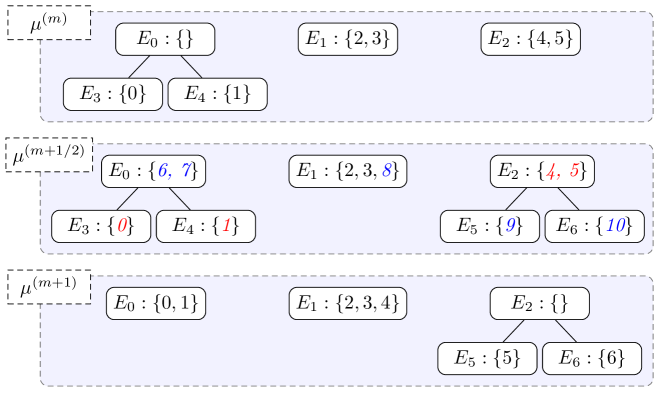
Figure 1: Computation of a global DOF mapping $\mu^{(m+1)}$ by Steps missingfnum@@desciitemStep 1 (Insertion of new DOFs). to missingfnum@@desciitemStep 3 (Removal of DOFs). of Definition 3.3, see Example 3.5 for details.

Example 3.5.

Figure 1 shows a hierarchical grid with three macro elements $E_{0},E_{1},E_{2}$ with $E_{0}$ having two children $E_{3},E_{4}$. The leaf level elements form the grid $\mathcal{G}^{(m)}=\{E_{i}\mid i=1,\ldots,4\};$ the global DOF numbers associated with each element are depicted inside the brackets. Here, level $0$ elements are assumed to hold at least two DOFs, while level $1$ elements shall have one DOF. Next, $E_{3}$ and $E_{4}$ are marked for coarsening, $E_{2}$ is marked for refinement, and $E_{1}$ gets assigned an additional DOF by local $p$-refinement. Newly inserted DOFs added in Step missingfnum@@desciitemStep 1 (Insertion of new DOFs). and DOFs to be removed in Step missingfnum@@desciitemStep 3 (Removal of DOFs). are printed in italics. During the modification phase the number of DOFs is enlarged to allow for the local projection of user data.

Remark 3.6 (Storage costs).

During the adaptation from $X^{(m)}$ to $X^{(m+1)}$ the maximum length of the global DOF vector equals $\lvert\mathcal{D}^{(m+1/2)}\rvert=\mathcal{O}(\lvert\mathcal{G}^{(m)}\cup\mathcal{G}^{(m+1)}\rvert).$ Taking into account the temporary storage used in Step missingfnum@@desciitemStep 2 (Restriction and prolongation of user data). the overall memory consumption of algorithm 3.3 is of order $\mathcal{O}(\lvert\mathcal{G}^{(m)}\cup\mathcal{G}^{(m+1)}\rvert+1).$

4 Using the dune-fem-hpdg module

In this section we describe the usage of the dune-fem-hpdg add-on module to the Dune-Fem finite element library. The module provides extensible reference implementations of adaptive discrete function spaces for implementing $p$- and $hp$-adaptive discontinuous finite element methods. First, we give a brief introduction to Dune-Fem and in particular its local mesh adaptation capabilities.

4.1 The Dune-Fem finite element library

The C++-library Dune-Fem provides a number of abstract interface classes representing discrete functions and discrete function spaces, local basis function sets, and DOF vectors and DOF mappings. These classes and their relationships are summarized in Figure 2. Here, a DiscreteFunction represents an element $u\in X(\mathcal{G}).$ A discrete function holds a global DOF vector

$$\bm{u}=(u_{0},\ldots,u_{N-1})$$

and is usually evaluated in local coordinates with respect to a given element $E\in\mathcal{G}$. The local DOF vector

$$(u_{\mu_{E}(0)},\ldots,u_{\mu_{E}(n_{E}-1)})$$

is initialized by the DofMapper, a class representing the family of local DOF mappings $\left(\mu_{E}\right)_{E\in\mathcal{G}}.$ Finally, a BasisFunctionSet represents the local basis function set $\mathcal{B}_{E}$, and the local function $u\mathord{\restriction}_{E}\in X(E)$ is given by

$$u\mathord{\restriction}_{E}=\sum_{i=0}^{n_{E}-1}u_{\mu_{E}(i)}\varphi_{E,i}.$$

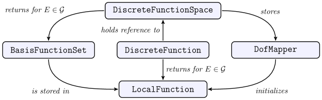
Figure 2: Interplay of the main interface classes in Dune-Fem representing discrete function spaces and discrete functions.

In most complex applications, more than one discrete function is in use. This poses some difficulty in adaptive simulations. A grid may be only be adapted once, and all discrete functions must be restricted and prolonged simultaneously. In Dune-Fem, a sole class, the DofManager, is responsible for starting the grid adaptation process. It resizes all DOF vectors and notifies DOF mappings about the update.

In case no user data must be restricted and prolonged no action is required. Otherwise, users must add discrete functions, containers, etc., to an AdaptationManager. This class is equipped with the necessary information (encapsulated in a RestrictProlong object) on how to locally project user data during adaptation. Listing 1 illustrates the adaptation process from a user perspective.

Listing 1: Sample code illustrating the automated restriction and prolongation of discrete functions under grid refinement in Dune-Fem.

⬇

1template <class DiscreteFunction>

2void adapt(DiscreteFunction &uh, unsigned int seed) {

3 // get grid (slightly simplified)

4 using Grid = typename DiscreteFunction::GridType;

5 Grid &grid = uh.grid();

6

7 // create adaptation manager (slightly simplified)

8 using RestrictProlong = RestrictProlongDefault<DiscreteFunction>;

9 using h_AdaptationManager = AdaptationManager<Grid, RestrictProlong>;

10 h_AdaptationManager h_adaptManager(RestrictProlong(uh));

11

12 // randomly mark leaf level grid elements for refinement/coarsening

13 default_random_engine engine(seed);

14 uniform_int_distribution<int> distribution(-1, 1);

15 for (const auto &element : elements(grid.leafGridView()))

16 grid.mark(distribution(engine), element);

17

18 // adapt discrete function

19 h_adaptManager.adapt();

20}

4.2 Discrete function spaces in dune-fem-hpdg

As illustrated in Figure 2 a DiscreteFunctionSpace assembles the local basis function sets and DOF mappings. The dune-fem-hpdg extends the list of available discrete function spaces available to users of Dune-Fem by the following $hp$-adaptive spaces:

fnum@@desciitemOrthogonalDiscontinuousGalerkinSpace

an implementation of the example finite element space 2.5,

fnum@@desciitemLegendreDiscontinuousGalerkinSpace

a discontinuous finite element space using product Legendre ansatz polynomials, i.e., $\mathcal{B}_{E,k}=\left\{\varphi_{\bm{\alpha}}\mid 0\leq\alpha_{i}\leq k,i=1,\ldots,d\right\},k\in\mathbb{N},$ with

$$\varphi_{\bm{\alpha}}(F_{E}(x))=\prod_{i=1}^{d}p_{\alpha_{i}}(x_{i})\quad(x\in R_{E}),$$

where $F_{E}:R_{E}\rightarrow E$ is an affine reference mapping and the $i$-th Legendre polynomial on the unit interval $[0,1]$ is defined by

$$p_{i}(x)=\frac{1}{i!}\frac{\mathrm{d}^{i}}{\mathrm{d}x^{i}}\bigl{[}(x^{2}-x)^{i}\bigr{]},$$

fnum@@desciitemAnisotropicDiscontinuousGalerkinSpace

a discontinuous space based on product Legendre polynomials as well; this implementation, however, allows for an adaptation in $p$ in each spatial direction.

We remark that the latter two spaces based on Legendre polynomials are restricted to cubic grids, i.e., $R_{E}=[0,1]^{d}$ for all $E\in\mathcal{G}$.

The discrete function spaces listed above differ in the choice of local basis function sets. They do, however, share the common base class hpDG::DiscontinuousGalerkinSpace providing almost all other functionality. In the same way, the dune-fem-hpdg module allows users to quickly setup new discrete function spaces. In order to do so, users must provide an implementation of the hpDG::BasisFunctionSets interface which represents a family of local basis function sets. This is explained in more detail in Appendix B.

The construction of the discontinuous finite element spaces in dune-fem-hpdg is in no way different from that of all other discrete function spaces in Dune-Fem. Listing 2 illustrates the initialization of an adaptive discrete function suitable for $hp$-adaptive simulations.

Listing 2: Construction of a discrete function space and a discrete function with dune-fem-hpdg suitable for $hp$-adaptive simulations.

⬇

1// create quadrilateral ALUGrid

2using Grid = ALUGrid<2, cube, nonconforming>;

3Grid grid(/*...*/);

4

5// select leaf level partition

6using GridPart = AdaptiveLeafGridPart<Grid>;

7GridPart gridPart(grid);

8

9// create scalar discrete function space

10const int order = 3;

11using DiscreteFunctionSpace = hpDG::OrthogonalDiscontinuousGalerkinSpace<

12 FunctionSpace<double, double 2, 1>, GridPart, order>;

13DiscreteFunctionSpace space(gridPart);

14

15// create discrete function

16using DiscreteFunction = AdaptiveDiscreteFunction<DiscreteFunctionSpace>;

17DiscreteFunction uh("uh", space);

4.3 An interface for local p-adaptation

Listing 3: Sample code illustrating the automated restriction and prolongation of discrete functions under modification of the local polynomial degree.

⬇

1template <class DiscreteFunction>

2void adapt(DiscreteFunction &uh, unsigned int seed) {

3 // get space (slightly simplified)

4 using DiscreteFunctionSpace =

5 typename DiscreteFunction::DiscreteFunctionSpaceType;

6 DiscreteFunctionSpace &space = uh.space();

7

8 // create adaptation manager

9 using Grid = typename DiscreteFunction::GridType;

10 using DataProjection = hpDG::DefaultDataProjection<DiscreteFunction>;

11 using p_AdaptationManager = hpDG::AdaptationManager<Grid, DataProjection>;

12 p_AdaptationManager p_adaptManager(DataProjection(uh));

13

14 // randomly mark grid (part) elements for p-adaptation

15 default_random_engine engine(seed);

16 uniform_int_distribution<int> distribution(0, space.order());

17 for (const auto &element : elements(uh.gridPart()))

18 space.mark(distribution(engine), element);

19

20 // adapt discrete function

21 p_adaptManager.adapt();

22}

The most important design decision we made in implementing the dune-fem-hpdg module was to split $h$- and $p$-refinement in two separate stages. Our reasoning is twofold. First, the software should support $h$-adaptive legacy code in the manner described above in Section 4.1. Second, this strategy allows for an arbitrary number of $h$-, $p$- and $hp$-adaptive discrete functions in single application and gives users the necessary freedom in complex applications. Standard use cases are easy to implement as will be shown in Section 5.

Any of the discrete function spaces in dune-fem-hpdg provides a set of extended interface methods for local $p$-adaptation. In most papers, $p$ denotes an integer, e.g., the polynomial order of a local approximation space. We slightly generalized this idea and allow $p$ to be of arbitrary type (the Key type), e.g., a vector of individual local polynomial degrees for each space direction. The $p$-adaptive interface mimicks that of the grid adaptation in Dune-.

⬇

1const DiscreteFunctionSpace::KeyType &key(

2 const DiscreteFunctionType::EntityType &entity) const;

3void DiscreteFunctionSpace::mark(

4 const DiscreteFunctionType::KeyType &key,

5 const DiscreteFunctionType::EntityType &element);

The first method returns the key currently assigned to a grid element, while mark allows for re-assigning a new key. In order for the changes to take effect, one of the following two adapt methods must be called.

⬇

1bool DiscreteFunctionSpace::adapt();

2template <DataProjection>

3bool DiscreteFunctionSpace::adapt(DataProjection &projection);

The necessary information on how to locally project data are encapsulated in a DataProjection. As in case of $h$-adaptation, however, users will not call these methods explicitly. Instead, the hpDG::AdaptationManager class handles the restriction and prolongation as illustrated by Listing 3. Note how closely the code resembles Listing 1 above on local mesh adaptation in Dune-Fem. In this particular example, a single discrete function is restricted and prolonged; however, the dune-fem-hpdg facilities may be provided with an arbitrary number of discrete functions and other user data. More information on the adaptation and the restriction and prolongation of custom user data can be found in Appendix B.

5 An hp-adaptive interior penalty Galerkin method

In this final section we want to illustrate in a complex application the capabilities and usage of the dune-fem-hpdg module. We will be concerned with the numerical solution of an elliptic PDE by means of an $hp$-adaptive symmetric interior penalty Galerkin (SIPG) scheme. First, we briefly revisit the $hp$-version of the SIPG method following the recent book by Dolejší and Feistauer [13, Chapter 7].

5.1 The hp-version of the SIPG method

Let $\Omega\subset\mathbb{R}^{2}$ be a bounded domain with Lipschitz boundary $\partial\Omega$. We consider the following elliptic model problem

$$-\Delta u =f\quad\text{in }\Omega,u =g\quad\text{on }\partial\Omega$$ (2)

for given source $f$ and boundary values $g$. The domain is discretized by a grid $\mathcal{G}$; for $E\in\mathcal{G}$ we denote the sets of interior and boundary intersections by

The sets of all interior and boundary intersections will be denoted by $\Gamma_{\mathit{int}}$ and $\Gamma_{\mathit{bnd}}$, respectively. We fix local polynomial degrees $\bm{k}=(k_{E})_{E\in\mathcal{G}}$ with $k_{E}\geq 1$ for all $E\in\mathcal{G}$ and consider the standard discontinuous finite element space

$$X^{\bm{k}}(\mathcal{G})=\{u\in L^{\infty}(\Omega)\mid u\mathord{\restriction}_{E}\in P^{k_{E}}(E)\text{ for all }E\in\mathcal{G}\}.$$

The jump of a discrete function $u\in X^{\bm{k}}(\mathcal{G})$ across an inter-element intersection $e\in\Gamma_{\mathit{int}}$, $e=E\cap E^{\prime}$, is defined by

$$\llbracket u\rrbracket(x)=\left(u\mathord{\restriction}_{E}\nu_{E}+u\mathord{\restriction}_{E^{\prime}}\nu_{E^{\prime}}\right)(x)\quad(x\in e),$$

where $\nu_{E}$ denotes a unit outer normal to $E\in\mathcal{G}$. The average of a discrete function is given by

$$\{u\}(x)=\frac{1}{2}\bigl{(}u\mathord{\restriction}_{E}+u\mathord{\restriction}_{E^{\prime}}\bigr{)}(x)\quad(x\in e).$$

For each intersection $e\in\Gamma_{\mathit{int}}\cup\Gamma_{\mathit{bnd}}$ we introduce the penalty parameter

$$\sigma_{e}=\begin{dcases}\gamma\frac{k_{E}^{2}+k_{E^{\prime}}^{2}}{2h_{e}}&\text{for }e=E\cap E^{\prime},\\ \gamma\frac{k_{E}^{2}}{h_{e}}&\text{for }e=\partial E\cap\partial\Omega,\end{dcases}$$

where $\gamma>0$ is a sufficiently large constant and $h_{e}$ denotes the diameter of $e$. Note that the penalty parameter depends on the local polynomial degrees. Now, let $B:X^{\bm{k}}(\mathcal{G})\times X^{\bm{k}}(\mathcal{G})\rightarrow\mathbb{R}$ be a bilinear form defined by

$$\begin{split}B(u,\psi)=&\sum_{E\in\mathcal{G}}\int_{E}\nabla u\cdot\nabla\psi\mathop{}\!\mathrm{d}x\\ &\quad-\sum_{e\in\Gamma_{\mathit{int}}}\int_{e}\llbracket u\rrbracket\{\nabla\psi\}+\llbracket\psi\rrbracket\{\nabla u\}\mathop{}\!\mathrm{d}s+\sum_{e\in\Gamma_{\mathit{int}}}\int_{e}\sigma_{e}\llbracket u\rrbracket\llbracket\psi\rrbracket\mathop{}\!\mathrm{d}s\\ &\quad-\sum_{e\in\Gamma_{\mathit{bnd}}}\int_{e}u(\nabla\psi\cdot\nu)+\psi(\nabla u\cdot\nu)\mathop{}\!\mathrm{d}s+\sum_{e\in\Gamma_{\mathit{bnd}}}\int_{e}\sigma_{e}u\psi\mathop{}\!\mathrm{d}s,\end{split}$$

and $l:X^{\bm{k}}(\mathcal{G})\rightarrow\mathbb{R}$ defined by

$$l(\psi)=\int_{\Omega}f\psi\mathop{}\!\mathrm{d}x-\sum_{e\in\Gamma_{\mathit{bnd}}}\int_{e}g(\nabla\psi\cdot\nu)\mathop{}\!\mathrm{d}s+\sum_{e\in\Gamma_{\mathit{bnd}}}\int_{e}\sigma_{e}g\psi\mathop{}\!\mathrm{d}s.$$

The bilinear form $B$ is continuous and coercive with respect to the energy norm $\lVert\cdot\rVert_{\mathit{DG}}:X^{\bm{k}}(\mathcal{G})\rightarrow\mathbb{R}$ defined by

$$\lVert u\rVert_{\mathit{DG}}^{2}=\sum_{E\in\mathcal{G}}\int_{E}\lvert\nabla u\rvert^{2}\mathop{}\!\mathrm{d}x+\sum_{e\in\Gamma_{\mathit{int}}}\int_{e}\sigma_{e}\llbracket u\rrbracket^{2}\mathop{}\!\mathrm{d}s+\sum_{e\in\Gamma_{\mathit{bnd}}}\int_{e}\sigma_{e}u^{2}\mathop{}\!\mathrm{d}s$$

provided the constant $\gamma$ is sufficiently large [13, Theorems 7.13 and 7.15]. This guarantees the existence and uniqueness of the weak solution $u_{h}\in X^{\bm{k}}(\mathcal{G})$ to the model problem (2) defined by

$$B(u_{h},\psi)=l(\psi)\quad(\psi\in X^{\bm{k}}(\mathcal{G})).$$ (3)

5.2 The hp-adaptive scheme

The first component in the construction of a fully $hp$-adaptive scheme is an a posteriori error indicator estimating the local approximation error. Of course, the local error indicators must be computable from the numerical solution $u_{h}$ and the given data $f,g$ alone. There is a growing body of literature on a posteriori error estimation, see, e.g., [12, 21, 32]. We implemented the following indicator from [24],

$$\begin{split}\eta_{E}^{2}=&\frac{{h_{E}}^{2}}{{k_{E}}^{2}}\int_{E}\bigl{(}\Pi_{E,k_{E}-1}(f+\Delta u_{h})\bigr{)}^{2}\mathop{}\!\mathrm{d}x\\ &\quad+\sum_{e\in\mathcal{I}_{\mathit{int}}(E)}\left\{\frac{h_{E}}{k_{E}}\int_{e}\bigl{(}\Pi_{e,k_{e}-1}\llbracket\nabla u_{h}\cdot\nu_{E}\rrbracket\bigr{)}^{2}\mathop{}\!\mathrm{d}s+\frac{{k_{E}}^{3}}{h_{E}}\int_{e}\llbracket u_{h}\rrbracket^{2}\mathop{}\!\mathrm{d}s\right\}\\ &\quad+\sum_{e\in\mathcal{I}_{\mathit{bnd}}(E)}\frac{{k_{E}}^{3}}{h_{E}}\int_{e}(u_{h}-g)^{2}\mathop{}\!\mathrm{d}s\quad(E\in\mathcal{G}).\end{split}$$ (4)

Here, $\Pi_{E,k_{E}-1}\text{ and }\Pi_{e,k_{e}-1}$ denote local $L^{2}$-projections onto the polynomial spaces of lower degree $P^{k_{E}-1}(E)$ and $P^{k_{e}-1}(e)$ with $k_{e}=\max\{k_{E},k_{E^{\prime}}\}$. It can be shown that

$$\lVert u-u_{h}\rVert_{\mathit{DG}}\leq\left(\sum_{E\in\mathcal{G}}\eta_{E}^{2}+\mathcal{O}(f,u_{h})\right)^{\frac{1}{2}},$$

where $\mathcal{O}(f,u_{h})$ denotes a data-oscillation term, see [24, Theorem 3.2] for details. Having computed the local error indicator we mark $E\in\mathcal{G}$ for refinement in either $h$ or $p$ if the local error indicator exceeds an upper bound $\eta^{*}$,

$$\eta_{E}<\eta_{*}=\mathit{TOL}/\lvert\mathcal{G}\rvert.$$

If no element is marked for further refinement we stop the iterative procedure.

Once a grid element has been identified for local adaptation it must be decided whether to refine in $h$ or $p$. Several strategies for this have been proposed in the literature, see, e.g., [11, 14, 22, 23, 29, 31]. We implemented the so-called Prior2P strategy described in [28] based on the following idea. A priori error estimates (see, e.g., [13, Theorem 7.20]) suggest that we should increase the local polynomial degree $k_{E}$ provided the exact is sufficiently smooth in $E\in\mathcal{G}$. A regularity indicator yields an estimate for the local Sobolev index $q_{E}$,

$$q_{E}=\max\{q\mid u\mathord{\restriction}_{E}\in H^{q}(E)\}\quad(E\in\mathcal{G}).$$

We increase the local polynomial order provided $k_{E}<q_{E}-1$; otherwise, we mark $E$ for local mesh refinement.

1:choose initial grid $\mathcal{G}$ and local polynomial degrees $\bm{k}=\left(k_{E}\right)_{E\in\mathcal{G}}$

2:for $m=0,1,\ldots$ do

3:     solve system (3) to compute $u_{h}\in X^{\bm{k}}(\mathcal{G})$

4:     for all elements $E\in\mathcal{G}$ do

5:          compute the local error indicator $\eta_{E}$ from (4)

6:     end for

7:     if $\left(\sum_{E\in\mathcal{G}}\eta_{E}^{2}\right)^{\frac{1}{2}}\leq\mathit{TOL}$ then

8:          stop

9:     end if

10:     for all elements $E\in\mathcal{G}$ do

11:          if $\eta_{E}<\eta_{*}$ then

12:               mark element $E$ for $h$-coarsening, if possible;

13:               otherwise, set $k_{E}\leftarrow\max\{k_{E}-1,k_{\textit{min}}\}$

14:          else if $\eta_{E}>\eta^{*}$ then

15:               compute estimate for the local Sobolev index $q_{E}$

16:               if $q_{E}>k_{E}+1$ then

17:                    set $k_{E}\leftarrow\min\{k_{E}+1,k_{\textit{max}}\}$

18:               else

19:                    mark element $E$ for $h$-refinement

20:               end if

21:          end if

22:     end for

23:     while adapting the grid $\mathcal{G}$ do

24:          restrict and prolong $u_{h}$ and $\bm{k}$ according to (5) and (6)

25:     end while

26:end for

Algorithm 1 Summary of the $hp$-adaptive SIPG method.

So far we have only discussed local $hp$-refinement. Assume now that for $E\in\mathcal{G}$ the estimated local approximation error is small, i.e.,

$$\eta_{E}\leq\eta_{*}\ll\eta^{*}.$$

We may decide to reduce the number of degrees of freedom by decreasing the local polynomial degree $k_{E}$ or by coarsening the grid. Mesh coarsening usually depends on a number of neighboring elements (e.g., the children of a common father element in a hierarchical grid) all being marked for grid coarsening. We take a rather hands-on approach and — if possible — always favor $h$- over $p$-coarsening. We remark that the regularity indicator implemented restricts the minimum local polynomial degree to $k_{\mathit{min}}=3$.

Finally, we need to address the restriction and prolongation of the vector of local polynomial degrees $\bm{k}$. Let $E\in\mathcal{G}^{(m+1)}\backslash\mathcal{G}^{(m)}$ be an element created during grid modification. We must define the local polynomial degree $k^{(m+1)}_{E}$ to be associated with the newly created element. In case $E$ results from local mesh refinement of $E^{\prime}\in\mathcal{G}^{(m)}$ we simply set

$$k^{(m+1)}_{E}=k^{(m)}_{E^{\prime}}$$ (5)

locally prolonging $\bm{k}^{(m)}$ to $\bm{k}^{(m+1)}$. If otherwise $E$ results from local mesh coarsening we locally restrict $\bm{k}^{(m)}$ to $\bm{k}^{(m+1)}$ by setting

$$k^{(m+1)}_{E}=\max_{\begin{subarray}{c}E^{\prime}\in\mathcal{G}^{(m)},\\ E^{\prime}\subset E\end{subarray}}k^{(m)}_{E^{\prime}}.$$ (6)

The complete $hp$-adaptive SIPG scheme is summarized in Algorithm 1.

5.3 Implementation details

The dune-fem-hpdg contains a reference implementation of the $hp$-adaptive SIPG scheme described above. For the computation of the numerical solution we relied on Dune- and the Dune-Fem discretization module. The latter provides sample implementations of continuous and discontinuous finite element methods including an SIPG method for fixed global polynomial degree $k$. For the solution of the linear system (3) we used the Iterative Solver Template Library (Dune-ISTL), a Dune- module developed by Blatt and Bastian [7, 8]. The $hp$-adaptive scheme requires for a locally adaptive grid. In all our experiments we used the Dune-ALUGrid module by Alkämper et al. [1], a Dune- add-on encapsulating the ALUGrid library by Schupp [30].

We want to give some details on the implementation in order to illustrate the $hp$-adaptation process. Listing 4 shows a sample implementation of the marking procedure (Lines 10 to 22 of Algorithm 1).

Listing 4: Implementation of Algorithm 1, Lines 10 to 22. Note that the given vector of polynomial degrees $k$ associated with the discontinuous finite element space $X^{(m)}$ is overridden.

⬇

1enum class Flag { Coarsen, None, Refine };

2

3template <class Grid, class ManagedArray, class Function>

4void mark(Grid &grid, ManagedArray &k, Function function) {

5 for (const auto &element : elements(grid.leafGridView())) {

6 // get refinement flag and estimated Sobolev index

7 Flag what;

8 int q;

9 tie(what, q) = function(element);

10

11 // mark grid/vector of local polynomial degrees for

12 // hp-refinement/coarsening

13 switch (what) {

14 case Flag::None:

15 break;

16 case Flag::Coarsen:

17 if (element.hasFather())

18 grid.mark(-1, element);

19 else if (k[element] > 3)

20 k[element] -= 1;

21 break;

22 case Flag::Refine:

23 if (k[element] < q - 1)

24 k[element] += 1;

25 else

26 grid.mark(1, element);

27 }

28 }

29}

Here, the parameter function is a callable object which returns a pair of a refinement flag and an estimate for the local Sobolev index for a given entity. The array k is an associative container of local polynomial degrees currently in use. In case an element is flagged for refinement or coarsening it is either marked for $h$- or $p$-adaptation; in the latter case we re-assign its local polynomial degree in k. The modification of the grid and the finite element space as well as the restriction and prolongation of the discrete data are shown in Listing 5.

Listing 5: Prolongation of the vector of polynomial degrees during grid adaptation. It is assumed that the function mark from Listing 4 has been called in advance.

⬇

1template <class DiscreteFunction, class ManagedArray>

2void adapt(DiscreteFunction &u, ManagedArray &k) {

3 // get discrete function space (slightly simplified)

4 using DiscreteFunctionSpace =

5 typename DiscreteFunction::DiscreteFunctionSpaceType;

6 DiscreteFunctionSpace &space = u.space();

7

8 // get hierarchical grid

9 using Grid = typename DiscreteFunctionSpace::GridType;

10 Grid &grid = space.grid();

11

12 // h-adaptation, restrict/prolong numerical solution and polynomial degrees

13 using RestrictProlong =

14 RestrictProlongDefaultTuple<DiscreteFunction, ManagedArray>;

15 using h_AdaptationManager = AdaptationManager<Grid, RestrictProlong>;

16 h_AdaptationManager h_AdaptManager(grid, RestrictProlong(u, k));

17 h_AdaptManager.adapt();

18

19 // equip discrete function space with new local polynomial degrees

20 for (const auto &element : elements(grid.leafGridView()))

21 space.mark(k[element], element);

22

23 // p-adaptation, restrict/prolong numerical solution

24 using DataProjection = hpDG::DefaultDataProjection<DiscreteFunction>;

25 using p_AdaptationManager =

26 hpDG::AdaptationManager<DiscreteFunctionSpace, DataProjection>;

27 p_AdaptationManager p_AdaptManager(space, DataProjection(u));

28 p_AdaptManager.adapt();

29}

The first input argument of adapt is the approximate solution $u_{h}^{(m)}\in X^{(m)}=X^{\bm{k}^{(m)}}(\mathcal{G}^{(m)}).$ First, the grid is adapted to its new state $\mathcal{G}^{(m+1)}$. The approximate solution and the container are restricted $\bm{k}^{(m)}$ by the usual Dune-Fem facilities. This yields the vector $\bm{k}^{(m+1)}$ and an intermediate projection $u_{h}^{(m+1/2)}\in X^{\bm{k}^{(m)}}(\mathcal{G}^{(m+1)}).$ In Lines 20 and 21 the finite element space is marked for the concluding $p$-adaptation. The subsequent restriction and prolongation is handled by dune-fem-hpdg. It yields the desired projection of $u_{h}^{(m)}$ onto $X^{(m+1)}$. The resulting function serves as initial guess in the solution of the next linear system (3).

5.4 Numerical results

We consider the homogeneous model problem to recover a prescribed solution given by

$$u(x,y)=r^{2/3}\sin(2\varphi/3)$$

in a domain with reentrant corner $\Omega=(-1,1)^{2}\backslash(0,-1)\times(1,0).$ We compute two series of numerical solutions $u^{(m)}_{h}$, $m=0,\ldots,8$, on an axis-aligned quadrilateral mesh and a triangular mesh. In each case the $hp$-adaptive SIPG scheme yields a sequence of locally adapted meshes and distributions of local polynomial degrees. The so-called $hp$-meshes are shown in Figures 4,5 and 6,7. Since the exact solution is known we can compute the approximation error

$$e_{h}^{(m)}=u-u_{h}^{(m)}.$$

In order to determine the convergence rate (EOC) we follow [13] and define

$$\mathrm{EOC}=-\frac{\log(\lVert e_{h}^{(m)}\rVert/\lVert e_{h}^{(m+1)}\rVert)}{\log((N^{(m)}/N^{(m+1)})^{1/d})},$$

where $N^{(m)}$ denotes the number of global DOFs. Another interesting quantity for evaluating the effectiveness of the adaptive scheme is the so-called effectivity index, defined as the ratio of the a posteriori error indicator error bound and the energy norm, i.e.,

$$\text{Eff. index}=\frac{\left(\sum_{E\in\mathcal{G}^{(m)}}\eta_{E}^{(m)^{2}}\right)^{\frac{1}{2}}}{\lVert e_{h}^{(m)}\rVert_{\mathit{DG}}}.$$

The effectivity index depends on the problem under consideration and the macro grid. Within the elements of given series of approximate solutions, however, the effectivity index should be a constant. The approximation errors, convergence rates, and effectivity indices for the model problem are shown in Tables 1 and 2. We encourage users to run the sample code themselves; the instructions can be found in Appendix A.

Appendix A Installing and running the software

In this appendix we describe how to download and install the dune-fem-hpdg module and how to reproduce the numerical results presented in Section 5.

A.1 Download of required Dune modules

The following Dune- modules are needed in order to build and run the examples:

1. the Dune- 2.4 core modules Dune-Common, Dune-Geometry, Dune-Grid, Dune-ISTL, and Dune-LocalFunctions ,

2. the Dune-ALUGrid library,

3. the Dune-Fem discretization module,

4. and the dune-fem-hpdg module.

Please make sure that you check out the Dune- 2.4 compatible (release) branches of Dune-ALUGrid, Dune-Fem, and dune-fem-hpdg.

A.2 Installation of the software

Before installing Dune- and its components please refer to the installation notes for a list of dependencies and required software. We assume all aforementioned Dune packages have been downloaded and saved to a single directory $DUNE. For the simultaneous build of all modules using CMake run the dunecontrol script, e.g., by

⬇

1cd $DUNE

2./dune-common/bin/dunecontrol all

Please refer to the installation notes for more information and on how to pass options to the build process.

A.3 Running the hp-adaptive sample code

We assume that Dune- has been configured using CMake. By default, binary executables will be built out-of-source, e.g., in a designated build directory build_cmake. The sources for the $hp$-adaptive SIPG method can be found in the subdirectory examples/poisson. In order to verify the results shown in Figures 4, 5 and Table 1 compile and run the test as follows

⬇

1cd $DUNE/dune-fem-hpdg/build-cmake

2cd ./examples/poisson

3make poisson_alugrid_cube_7

4./poisson_alugrid_cube_7 ./reentrantcorner.dgf

The results for the triangular grid shown in Figures 6, 7 and Table 2 may be reproduced from running

⬇

1make poisson_alugrid_simplex_7

2./poisson_alugrid_simplex_7 ./reentrantcorner.dgf

If an MPI implementation was found during the build process the tests may be run in parallel in an analogous way.

Appendix B Advanced user API

In this final appendix we want to describe two advanced aspects of the dune-fem-hpdg module, the definition of custom data projections for the restriction and prolongation of user data and the implementation of new discontinuous finite element spaces based on user-defined local basis function sets.

B.1 Restriction and prolongation of custom user data

Remember from Section 4.3 that the restriction and prolongation of data in dune-fem-hpdg is handled by the hpDG::AdaptationManager class. Any input must be encapsulated in a DataProjection object.

⬇

1using DataProjection = hpDG::DefaultDataProjection<Data>;

2hpDG::AdaptationManager<DiscreteFunctionSpace, DataProjection> p_AdaptManager(

3 space, DataProjection(u));

A DataProjection is a callable object encapsulating the data $u^{(m)}$ associated with the discrete function space $X^{(m)}$. Any such projection must inherit from the base class hpDG::DataProjection, as illustrated by the following listing.

⬇

1template <class DiscreteFunctionSpace, class Data>

2class DefaultDataProjection

3 : public DataProjection<DiscreteFunctionSpace,

4 DefaultDataProjection<Data> > {

5 public:

6 using BasisFunctionSetType =

7 typename DiscreteFunctionSpace::BasisFunctionSetType;

8 using EntityType = typename BasisFunctionSetType::EntityType;

9

10 void DataProjection::operator()(const EntityType &element,

11 const BasisFunctionSetType &former,

12 const BasisFunctionSetType &future,

13 const vector<size_t> &origin,

14 const vector<size_t> &destination);

15};

The method operator() is expected to evaluate the local projection $\Pi^{(m+1)}u^{(m)}\mathord{\restriction}_{E}$ for each element $E\in\mathcal{G}^{(m)}\cap\mathcal{G}^{(m+)1}$. Its input arguments are

1. the grid element $E$,

2. the former and future local basis function sets $\left(\varphi_{E,i}^{(m)}\right)_{i=0,\ldots,n_{E}^{(m)}-1},~{}\left(\varphi_{E,i}^{(m+1)}\right)_{i=0,\ldots,n_{E}^{(m+1)}-1},$

3. and the DOF indices $(\mu^{(m)}(E,i))_{i=0,\ldots,n_{E}^{(m)}-1},~{}(\mu^{(m+1/2)}(E,i))_{i=0,\ldots,n_{E}^{(m+1)}-1}.$

Note that this is all information needed in order to implement the local $L^{2}$-projection from Example 3.1.

B.2 Setup of new adaptive discontinuous finite element spaces

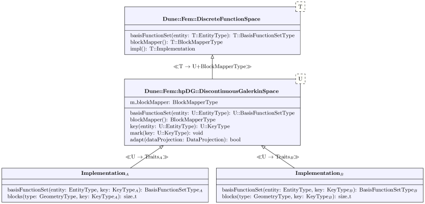
Figure 3: Class diagram for derived implementations of $hp$-adaptive discontinuous finite element spaces inheriting from the hpDG::DiscontinuousGalerkinSpace base class.

As described in Section 4.2 the discrete function spaces provided by dune-fem-hpdg inherit from a common base class implementing almost all functionality, see Figure 3. In the same way, users may setup new discontinuous finite element spaces. To do so, users need to provide an implementation of the hpDG::BasisFunctionSets interface which contains essentially two methods.

⬇

1template <class BasisFunctionSet, class Key>

2class BasisFunctionSets {

3 public:

4 using EntityType = typename BasisFunctionSet::EntityType;

5

6 BasisFunctionSet basisFunctionSet(const EntityType &entity,

7 const Key &key) const;

8 size_t blocks(GeometryType type, const Key &key) const;

9 // ...

10};

Remember that a GeometryType is a Dune- data type that identifies a reference element. Given a grid element $E$ with reference element $R_{E}$ and a key $k$ the method basisFunctionSet returns the corresponding local basis function set $\mathcal{B}_{E,k}$. We assume that the size of the local basis function set only depends on $R_{E}$ and $k$. Then, the method blocks returns the number of blocks to be reserved for $\mathcal{B}_{E,k}$. A BlockMapper is a Dune-Fem class representation a DOF mapping; in case of a scalar function spaces the number of blocks coincides with the number of local basis functions in $\mathcal{B}_{E,k}$.

Users may inherit from the base implementation hpDG::DiscontinuousGalerkinSpace. Alternatively, the convenience function make_space immediately constructs a discrete function space, given a grid part, the family of basis function sets, and a default key for initializing the space.

⬇

1template <class GridPart, class BasisFunctionSets>

2std::unique_ptr<DefaultDiscontinuousGalerkinSpace<BasisFunctionSets> >

3make_space(GridPart &gridPart, const BasisFunctionSets &basisFunctionSets,

4 const typename BasisFunctionSets::KeyType &key);

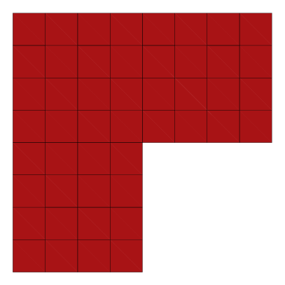
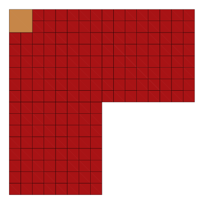
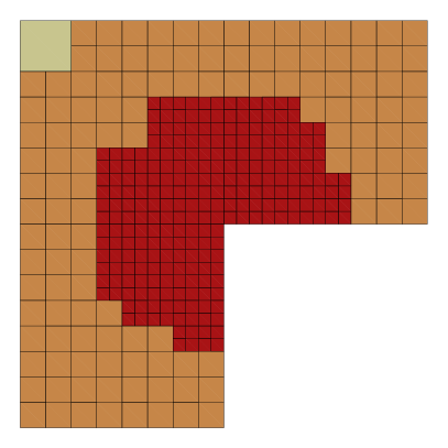
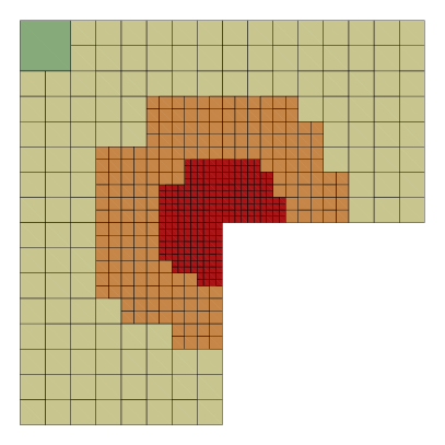
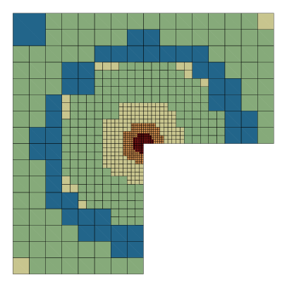
Figure 4: $hp$-meshes generated by the $hp$-adaptive SIPG method when solving the reentrant corner benchmark problem on a quadrilateral grid.

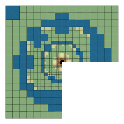
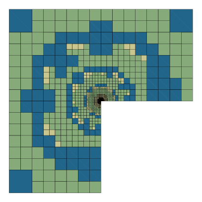
Figure 5: $hp$-meshes generated by the $hp$-adaptive SIPG method when solving the reentrant corner benchmark problem on a quadrilateral grid.

Table 1: Number of elements and degrees of freedom, errors and convergence rates, and effectivity index for the series of quadrilateral grids depicted in Figures 4 and 5.

Elements	DoFs	$\lVert u-u_{h}\rVert_{L^{2}}$	EOC	$\lVert u-u_{h}\rVert_{\mathit{DG}}$	EOC	$\left(\sum\eta_{E}^{2}\right)^{\frac{1}{2}}$	Eff. index
$48$	$480$	$2.30\text{\times}{10}^{-03}$	—	$2.22\text{\times}{10}^{-01}$	—	$3.30\text{\times}{10}^{-01}$	$1.49$
$189$	$1895$	$8.56\text{\times}{10}^{-04}$	$1.4$	$1.39\text{\times}{10}^{-01}$	$0.7$	$2.08\text{\times}{10}^{-01}$	$1.49$
$378$	$4416$	$3.25\text{\times}{10}^{-04}$	$2.3$	$8.77\text{\times}{10}^{-02}$	$1.1$	$1.31\text{\times}{10}^{-01}$	$1.49$
$567$	$8008$	$1.25\text{\times}{10}^{-04}$	$3.2$	$5.52\text{\times}{10}^{-02}$	$1.6$	$8.23\text{\times}{10}^{-02}$	$1.49$
$756$	$12\,846$	$4.85\text{\times}{10}^{-05}$	$4.0$	$3.48\text{\times}{10}^{-02}$	$2.0$	$5.19\text{\times}{10}^{-02}$	$1.49$
$945$	$18\,376$	$1.90\text{\times}{10}^{-05}$	$5.2$	$2.19\text{\times}{10}^{-02}$	$2.6$	$3.27\text{\times}{10}^{-02}$	$1.49$
$1104$	$22\,964$	$7.47\text{\times}{10}^{-06}$	$8.4$	$1.38\text{\times}{10}^{-02}$	$4.1$	$2.06\text{\times}{10}^{-02}$	$1.49$
$1269$	$27\,480$	$2.95\text{\times}{10}^{-06}$	$10.4$	$8.70\text{\times}{10}^{-03}$	$5.1$	$1.30\text{\times}{10}^{-02}$	$1.49$
$1464$	$32\,712$	$1.17\text{\times}{10}^{-06}$	$10.6$	$5.48\text{\times}{10}^{-03}$	$5.3$	$8.17\text{\times}{10}^{-03}$	$1.49$

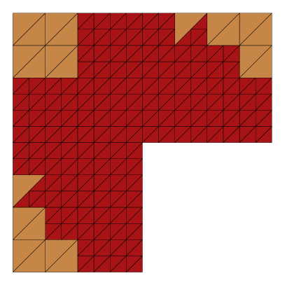
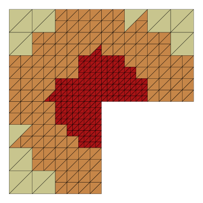
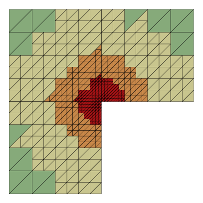
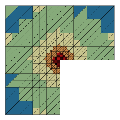
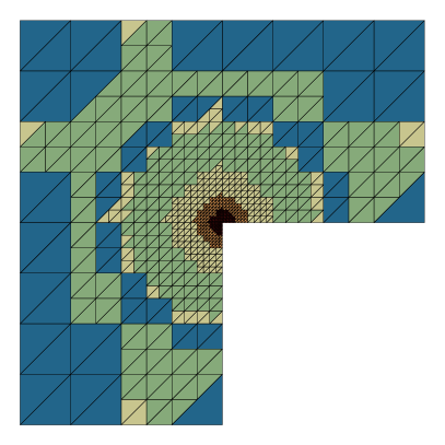
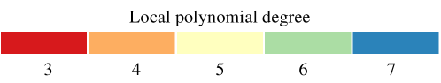
Figure 6: $hp$-meshes generated by the $hp$-adaptive SIPG method when solving the reentrant corner benchmark problem on an triangular grid.

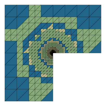
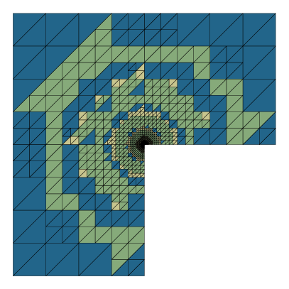
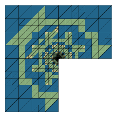
Figure 7: $hp$-meshes generated by the $hp$-adaptive SIPG method when solving the reentrant corner benchmark problem on an triangular grid.

Table 2: Number of elements and degrees of freedom, errors and convergence rates, and effectivity index for the series of triangular grids depicted in Figures 6 and 7.

Elements	DoFs	$\lVert u-u_{h}\rVert_{L^{2}}$	EOC	$\lVert u-u_{h}\rVert_{\mathit{DG}}$	EOC	$\left(\sum\eta_{E}^{2}\right)^{\frac{1}{2}}$	Eff. index
$96$	$960$	$1.08\text{\times}{10}^{-03}$	—	$2.31\text{\times}{10}^{-01}$	—	$3.04\text{\times}{10}^{-01}$	$1.32$
$318$	$3290$	$4.09\text{\times}{10}^{-04}$	$1.6$	$1.44\text{\times}{10}^{-01}$	$0.8$	$1.92\text{\times}{10}^{-01}$	$1.33$
$558$	$6930$	$1.57\text{\times}{10}^{-04}$	$2.6$	$9.06\text{\times}{10}^{-02}$	$1.2$	$1.21\text{\times}{10}^{-01}$	$1.33$
$798$	$12\,014$	$6.08\text{\times}{10}^{-05}$	$3.4$	$5.70\text{\times}{10}^{-02}$	$1.7$	$7.60\text{\times}{10}^{-02}$	$1.33$
$1038$	$18\,690$	$2.37\text{\times}{10}^{-05}$	$4.3$	$3.59\text{\times}{10}^{-02}$	$2.1$	$4.79\text{\times}{10}^{-02}$	$1.33$
$1227$	$24\,137$	$9.33\text{\times}{10}^{-06}$	$7.3$	$2.26\text{\times}{10}^{-02}$	$3.6$	$3.02\text{\times}{10}^{-02}$	$1.34$
$1464$	$30\,643$	$3.68\text{\times}{10}^{-06}$	$7.8$	$1.42\text{\times}{10}^{-02}$	$3.9$	$1.90\text{\times}{10}^{-02}$	$1.34$
$1716$	$37\,871$	$1.46\text{\times}{10}^{-06}$	$8.8$	$8.97\text{\times}{10}^{-03}$	$4.4$	$1.20\text{\times}{10}^{-02}$	$1.34$
$1899$	$42\,361$	$5.76\text{\times}{10}^{-07}$	$16.5$	$5.65\text{\times}{10}^{-03}$	$8.2$	$7.54\text{\times}{10}^{-03}$	$1.34$