Thermodynamics in $f(R,R_{\alpha\beta}R^{\alpha\beta},\phi)$ theory of gravity

Abstract

First and second laws of black hole thermodynamics are examined at the apparent horizon of FRW spacetime in $f(R,R_{\alpha\beta}R^{\alpha\beta},\phi)$ gravity, where $R$, $R_{\alpha\beta}R^{\alpha\beta}$ and $\phi$ are the Ricci scalar, Ricci invariant and the scalar field respectively. In this modified theory, Friedmann equations are formulated for any spatial curvature. These equations can be presented into the form of first law of thermodynamics for $T_{h}d\hat{S}_{h}+T_{h}d_{i}\hat{S}_{h}+WdV=dE$, where $d_{i}\hat{S}_{h}$ is an extra entropy term because of the non-equilibrium presentation of the equations and $T_{h}d\hat{S}_{h}+WdV=dE$ for the equilibrium presentation. The generalized second law of thermodynamics (GSLT) is expressed in an inclusive form where these results can be represented in GR $f(R)$ and $f(R,\phi)$ gravities. Finally to check the validity of GSLT, we take some particular models and produce constraints of the parameters.

Keywords: Modified gravity; Dark energy theory; Thermodynamics.
PACS: 04.50.Kd; 95.36.+x; 04.70.Dy.

1 Introduction

The cosmological observations which leads to the recent accelerating expansion of the universe are weak lensing [1], large scale structure [2], cosmic microwave background (CMB) radiation [3, 4], Type Ia Supernovae [5] and baryon acoustic oscillations [6]. To explain the cosmic acceleration of the universe, two classical approaches are followed: first is to use General Relativity (GR) and introduce dark energy [7, 8]; and the second is modified theories of gravity, e.g., $f(R)$ gravity. The modified gravity theories have attain a great attention to study the current cosmic acceleration [3].

The first studies in black hole thermodynamics was done in 1970s, when physicists were thinking that there must be some connection among Einstein equations and thermodynamics because of the linkage between horizon area (geometric quantity) and entropy (thermodynamical quantity) of black holes. At that time, those thermodynamic studies were focused in the context of black hole in which the surface gravity (geometric quantity) is associated with its temperature (thermodynamical quantity) and the first law of thermodynamics (FLT) is satisfied by these quantities [9]. By the discovery of black hole thermodynamics, it was shown that gravitation and thermodynamics are deeply connected [10]. The Hawking temperature of apparent horizon (defined in proportionality relation with $K_{sg}$ surface gravity) and horizon entropy $S=A/4G$ fulfil the first law of thermodynamics [9, 11]. In 1995, using that the entropy is proportional to the horizon area of the BH and the first law of thermodynamics $\delta Q=TdS$, Jacobson [12] was able to derive the Einstein’s equations. For radiation dominated (FRW) universe, Verlinde discovered that the Friedmann equation can be recomposed in the form like the Cardy-Verlinde formula [13]. In higher-dimensional spacetime, this formula represents an entropy relation for a conformal field theory. It can be observed that radiation can be described by a conformal field theory. Therefore, thermodynamics of radiation in the universe has been formulated with the help of entropy formula can also be write in the form of Friedmann equation, which describes the dynamics of spacetime. Further, Verlinde discovered the relation between thermodynamics and Einstein’s equations. The discussion related to the relation between thermodynamics and the Einstein’s equation was done in [14].

The connection between the first law of thermodynamics (FLT) and the field equations in Einstein and modified gravities has been extensively studied in literature. Padmanabhan [15] developed such connection in Einstein gravity for spherically symmetric BH and showed that the field equations can be expressed in the form of FLT, $dE+PdV=TdS$. Such study is also executed in Lanczos-Lovelock gravity for spherically symmetric and general static spacetimes [16]. Applying the first law of thermodynamics to the apparent horizon of FRW universe and assuming the geometric entropy given by a quarter of the apparent horizon area, Cai and Kim derived the Friedmann equations which describes the dynamics of universe with any spatial curvature [17]. The relation between the Friedmann equations with the first law of thermodynamics for scalar-tensor gravity and $f(R)$ gravity is discussed by Akbar [18]. To satisfy the GSLT constraints and conditions imposed on cosmological future horizon $R_{h}$, Hubble parameter $H$, and the temperature $T$, in a phantom-dominated universe are described in [19]. Akbar [21] has shown that the differential form of Friedmann equations of FRW universe filled with a viscous fluid can be rewritten as a similar form of the first law of thermodynamics at the apparent horizon of FRW universe. In [23], authors discussed the existence of Reissner-Nordstr m and Kerr-Newman black holes in $f(R)$ theories and also explored their thermodynamics properties $f(R)$ theories and extended electromagnetic theories. Bamba has studied the first and second laws of thermodynamics of the apparent horizon in $f(R)$ gravity in the Palatini formalism [24, 25]. He also explored both nonequilibrium and equilibrium descriptions of thermodynamics in $f(R)$ gravity and conclude that equilibrium framework is more transparent than the non-equilibrium one. In [26] the laws of thermodynamics are studied by Wu for the generalized $f(R)$ gravity with curvature matter coupling in spatially homogeneous, isotropic FRW universe whose results shows that the field equations of the generalized $f(R)$ gravity with curvature matter coupling can be cast to the form of the first law of thermodynamics with the the entropy production terms and the GSLT can be given by considering the FRW universe filled only with ordinary matter enclosed by the dynamical apparent horizon with the Hawking temperature.

Further, the laws of thermodynamics at the apparent horizon of FRW spacetime in modified gravities involving non-minimal matter geometry coupling are discussed in [27]-[29]. In $f(R,T)$ and $f(R,T,Q)$ gravities it was found that the picture of equilibrium thermodynamics is not feasible in these theories, so the non-equilibrium treatment is used to study the laws of thermodynamics in both forms of the energy-momentum tensor of dark components. Recently, Huang et al. [30], presented the thermodynamic laws for the scalar-tensor theory with non-minimally derivative coupling.

In this paper, the horizon entropy is constructed from the first law of thermodynamics corresponding to the Friedmann equations in the context of $f(R,R_{\alpha\beta}R^{\alpha\beta},\phi)$ gravity. We explore the generalized second law of thermodynamics (GSLT) and find out the necessary condition for its validity in preview of some well known models. The paper is organized as follows: In Sec. 2, we review $f(R,R_{\alpha\beta}R^{\alpha\beta},\phi)$ gravity and formulate the field equations of FRW universe. Sec. 3 is devoted to study the non-equilibrium description of first and second laws of thermodynamics. In Sec. 4, the validity of GSLT for different models are discussed. Sec. 5 is devoted to study the equilibrium description of first and second laws of thermodynamics. Finally in Sec. 6 we conclude our results. Throughout the paper we will use the metric signature $(-,+,+,+)$, $c=1$, $\kappa=8\pi G$ and that the Ricci tensor $R_{\mu\nu}=R^{\sigma}{}_{\mu\sigma\nu}$.

2 $f(R,R_{\alpha\beta}R^{\alpha\beta},\phi)$ gravity

Scalar tensor modified theories of gravity which are based on non-minimal coupling between matter and the geometry, have had very interesting applications in the thermodynamics context (See for instance [31]). Let us consider a generic theory based on a smooth arbitrary function $f(R,R_{\alpha\beta}R^{\alpha\beta},\phi)$ on its arguments, where $R$, $R_{\alpha\beta}R^{\alpha\beta}\equiv Y$ and $\phi$ are the Ricci scalar, the Ricci invariant and the scalar field respectively within a scalar tensor context. The action of this modified theory reads [32],

$$S_{m}=\int d^{4}x\sqrt{-g}\left[\frac{1}{\kappa}\left(f\left(R,R_{\alpha\beta}R^{\alpha\beta},\phi\right)+\omega(\phi)\phi_{;\alpha}\phi^{;\alpha}\right)+\mathcal{L}_{m}\right],$$ (1)

where $\mathcal{L}_{m}$ and $\omega(\phi)$ are the matter Lagrangian density and a generic function of the scalar field $\phi$ respectively.

By varying the action (1) with respect to metric $g_{\mu\nu}$, the field equations obtained are:

$$f_{R}R_{\mu\nu}-\frac{1}{2}\left(f+\omega(\phi)\phi_{;\alpha}\phi^{;\alpha}\right)g_{\mu\nu}-f_{R;\mu\nu}+g_{\mu\nu}\Box f_{R}+2f_{Y}R_{\mu}^{\alpha}R_{\alpha\nu}$$ (2)

$$-2[f_{Y}R^{\alpha}_{(\mu}]_{;\nu)\alpha}+\Box[f_{Y}R_{\mu\nu}]+[f_{Y}R_{\alpha\beta}]^{;\alpha\beta}g_{\mu\nu}+\omega(\phi)\phi_{;\mu}\phi_{;\nu}=\kappa T_{\mu\nu}^{(m)},$$

where $\Box=g^{\mu\nu}\nabla_{\mu}\nabla_{\nu}$, $f_{R}=\partial f/\partial R$ and $f_{Y}=\partial f/\partial Y$. The energy-momentum tensor for a perfect fluid is defined as

$$T_{\mu\nu}^{(m)}=(\rho_{m}+p_{m})u_{\mu}u_{\nu}+p_{m}g_{\mu\nu},$$ (3)

where $p_{m}$, $\rho_{m}$ and $u_{\mu}$ are the pressure, energy density and the four velocity of the fluid respectively. Hereafter, we will assume that the matter of the universe has zero pressure $p_{m}=0$ (dust). An effective Einstein field equation from Eq. (2) can be written as

$$R_{\mu\nu}-\frac{1}{2}Rg_{\mu\nu}=8\pi G_{eff}T_{\mu\nu}^{(m)}+T_{\mu\nu}^{(d)},$$ (4)

where

$$G_{eff}=\frac{G}{f_{R}}\,,$$ (5)

where $G_{eff}$ is the effective gravitational matter and

$$T_{\mu\nu}^{(d)}=\frac{1}{f_{R}}\bigg{[}-\frac{1}{2}Rg_{\mu\nu}f_{R}+\frac{1}{2}\left(f+\omega(\phi)\phi_{;\alpha}\phi^{;\alpha}\right)g_{\mu\nu}+f_{R}{}_{;\mu\nu}-g_{\mu\nu}\Box f_{R}-2f_{Y}$$

$$\times R_{\mu}^{\alpha}R_{\alpha\nu}+2[f_{Y}R^{\alpha}_{(\mu}]_{;\nu)\alpha}-\Box[f_{Y}R_{\mu\nu}]-[f_{Y}R_{\alpha\beta}]^{;\alpha\beta}g_{\mu\nu}-\omega(\phi)\phi_{;\mu}\phi_{;\nu}\bigg{]},$$ (6)

represents an effective energy-momentum tensor related with all the new terms of the theory. The metric describing the FRW universe is

$$ds^{2}=h_{\alpha\beta}dx^{\alpha}dx^{\beta}+\tilde{r}^{2}d\Omega^{2},$$ (7)

with the 2-dimensional metric $h_{\alpha\beta}=\textrm{diag}\left(-1,\frac{a(t)^{2}}{1-kr^{2}}\right)$, $(x^{0},x^{1})=(t,r)$, $a(t)$ is the scale factor and $k=\pm 1,0$ is the spacial curvature. The second term is $\tilde{r}=a(t)r$ and $d\Omega^{2}=d\theta^{2}+\sin\theta^{2}d\varphi^{2}$ is the 2-dimensional sphere with unit radius. The gravitational field equations for the metric (7) are given by

$$3\left(H^{2}+\frac{k}{a^{2}}\right) = 8\pi G_{eff}\rho_{m}+\frac{1}{f_{R}}\bigg{[}\frac{1}{2}\left(Rf_{R}-f\right)-\frac{1}{2}\omega(\phi)\dot{\phi}^{2}$$ (8)

$$-3H\partial_{t}f_{R}-6H\big{(}2\dot{H}+3H^{2}+\frac{k}{a^{2}}\big{)}\partial_{t}f_{Y}$$

$$-f_{Y}\bigg{(}\dddot{H}+4H\ddot{H}+6\dot{H}H^{2}-2H^{4}-\frac{4kH^{2}}{a^{2}}\bigg{)}\bigg{]}\,,$$

$$-\left(2\dot{H}+3H^{2}+\frac{k}{a^{2}}\right) = \frac{1}{f_{R}}\bigg{[}\frac{1}{2}\left(f-Rf_{R}\right)-\frac{1}{2}\omega(\phi)\dot{\phi}^{2}+\partial_{tt}f_{R}+2H\partial_{t}f_{R}$$ (9)

$$+\left(4\dot{H}+6H^{2}+\frac{2k}{a^{2}}\right)\partial_{tt}f_{Y}+4H\bigg{(}\dot{H}+3H^{2}$$

$$+\frac{2k}{a^{2}}\bigg{)}\partial_{t}f_{Y}+f_{Y}\bigg{(}4\dddot{H}+20H\ddot{H}+10\dot{H}H^{2}$$

$$+16\dot{H}^{2}-18H^{4}-\frac{18k\dot{H}}{a^{2}}-\frac{20kH^{2}}{a^{2}}-\frac{18k^{2}}{a^{4}}\bigg{)}\bigg{]}\,.$$

Here, dots and $\partial_{t}$ represent total derivation and partial derivation with respect to the cosmic time $t$ and $H=\dot{a}/a$ is the Hubble parameter. These equations can be rewritten as

$$3\left(H^{2}+\frac{k}{a^{2}}\right) = 8\pi G_{eff}(\rho_{m}+\rho_{d})\,,$$ (10)

$$-2\left(\dot{H}-\frac{k}{a^{2}}\right) = 8\pi G_{eff}\left(\rho_{m}+\rho_{d}+p_{d}\right),$$ (11)

where $\rho_{d}$ and $p_{d}$ are the energy density and pressure of dark components with $G=f_{R}G_{eff}$, are given by

$$\rho_{d} = \frac{1}{8\pi G}\bigg{[}\frac{1}{2}\left(Rf_{R}-f\right)-\frac{1}{2}\omega(\phi)\dot{\phi}^{2}-3H\partial_{t}f_{R}-6H\bigg{(}2\dot{H}+3H^{2}+\frac{k}{a^{2}}\bigg{)}$$ (12)

$$\times\partial_{t}f_{Y}-f_{Y}\bigg{(}\dddot{H}+4H\ddot{H}+6\dot{H}H^{2}-2H^{4}-\frac{4kH^{2}}{a^{2}}\bigg{)}\bigg{]},$$

$$p_{d} = \frac{1}{8\pi G}\bigg{[}\frac{1}{2}\left(f-Rf_{R}\right)-\frac{1}{2}\omega(\phi)\dot{\phi}^{2}+\partial_{tt}f_{R}+2H\partial_{t}f_{R}+\bigg{(}4\dot{H}+6H^{2}$$ (13)

$$+\frac{2k}{a^{2}}\bigg{)}\partial_{tt}f_{Y}+4H\bigg{(}\dot{H}+3H^{2}+\frac{2k}{a^{2}}\bigg{)}\partial_{t}f_{Y}+f_{Y}\bigg{(}4\dddot{H}+20H\ddot{H}$$

$$+10\dot{H}H^{2}+16\dot{H}^{2}-18H^{4}-\frac{18k\dot{H}}{a^{2}}-\frac{20kH^{2}}{a^{2}}-\frac{8k^{2}}{a^{4}}\bigg{)}\bigg{]}.$$

For a dark fluid, the equation of state (EoS) parameter $\omega_{d}$ can be derived as $(\omega_{d}=\frac{p_{d}}{\rho_{d}})$

$$\omega_{d} = -1+\frac{1}{\rho_{d}}\bigg{[}-\omega(\phi)\dot{\phi}^{2}+\partial_{tt}\Psi-H\partial_{t}\Psi+\bigg{(}4\dot{H}+6H^{2}+\frac{2k}{a^{2}}\bigg{)}\partial_{tt}f_{Y}$$ (14)

$$-2H\bigg{(}4\dot{H}+3H^{2}+\frac{k}{a^{2}}\bigg{)}\partial_{t}f_{Y}+f_{Y}\bigg{(}3\dddot{H}+16H\ddot{H}+4\dot{H}H^{2}+16\dot{H}^{2}$$

$$-16H^{4}-\frac{18k\dot{H}}{a^{2}}-\frac{16kH^{2}}{a^{2}}-\frac{8k^{2}}{a^{4}}\bigg{)}\bigg{]}.$$

For ordinary matter, the semi-conservation equation is given by

$$\dot{\rho}+3H\rho=q.$$ (15)

For dark component, the conservation equation is given by

$$\dot{\rho}_{d}+3H(\rho_{d}+p_{d}) = q_{d},$$ (16)

$$\dot{\rho}_{\rm total}+3H(\rho_{\rm total}+p_{\rm total}) = q_{\rm total},$$ (17)

where $\rho_{\rm total}=\rho_{m}+\rho_{d}$, $p_{\rm total}=p_{m}+p_{d}$, $q_{d}$ is the energy exchange term of dark components and $q_{\rm total}=q+q_{d}$ is the total energy exchange term. Substituting Eq’s. (10) and (11) in the above equation, we have

$$q_{\rm total}=\frac{3}{8\pi G}\left(H^{2}+\frac{k}{a^{2}}\right)\partial_{t}f_{R}.$$ (18)

The energy exchange term for $f(R)$ gravity can be recovered by setting $f(R,Y,\phi)=f(R)$. In GR, by choosing $f(R,Y,\phi)=R$ we get $q_{\rm total}=0$.

3 Generalized Thermodynamics laws with non-equilibrium description

Here, we discuss the first and second laws of thermodynamics at the apparent horizon of FRW universe in a more general $f(R,Y,\phi)$ gravity.

3.1 First Law of Thermodynamics

In this section, we analyse the validity of the first law of thermodynamics at the apparent horizon in a FRW universe for $f(R,Y,\phi)$ gravity. The dynamical apparent horizon is derived by the relation $h^{\alpha\beta}\partial_{\alpha}\tilde{r}\partial_{\beta}\tilde{r}=0$ from which we have that the radius of apparent horizon is $\tilde{r}_{A}=\left(H^{2}+k/a^{2}\right)^{-\frac{1}{2}}.$ By taking time derivatives in $\tilde{r}_{A}$ and using Eq. (11), we obtain

$$f_{R}d\tilde{r}_{A}=4\pi GH\tilde{r}_{A}^{3}(\hat{\rho}_{\rm total}+\hat{p}_{\rm total})dt\,,$$ (19)

where $\hat{\rho}_{\rm total}=\hat{\rho_{m}}+\hat{\rho_{d}}$ and $\hat{p}_{\rm total}=\hat{p_{d}}$ are the total energy density and total pressure respectively. Here, $d\tilde{r}_{A}$ represents the infinitesimal change in the radius of the apparent horizon during an infinitesimal time interval $dt$. The temperature of the apparent horizon is defined as $T_{h}=|K_{sg}|/(2\pi)$, where $K_{sg}$ is the surface gravity given by [17]

$$K_{sg}=-\frac{1}{\tilde{r}_{A}}\Big{(}1-\frac{\dot{\tilde{r}}_{A}}{2H\tilde{r}_{A}}\Big{)}\,.$$ (20)

In GR, Bekenstein and Hawking defined the horizon entropy by the relation $S_{h}=A/4G$, where $A$ is the area of the apparent horizon defined by $A=4\pi\tilde{r}_{A}^{2}$ [9, 10, 11]. In the literature of modified theories of gravity, Wald introduced the horizon entropy with a Noether charge [33]. This quantity can be obtained by varying the Lagrangian density of the modified theory with respect to Riemann tensor. This entropy is defined as $\hat{S_{h}}=A/4G_{eff}$ [34], where $G_{eff}$ is the effective gravitational coupling. The Wald’s entropy in $f(R,Y,\phi)$ gravity is defined as

$$\hat{S_{h}}=\frac{f_{R}A}{4G}\,.$$ (21)

By differentiating Eq. (21) and using (19), we have

$$\frac{1}{2\pi\tilde{r}_{A}}d\hat{S_{h}}=4\pi\tilde{r}_{A}^{3}\left(\hat{\rho}_{\rm total}+\hat{p}_{\rm total}\right)Hdt+\frac{\tilde{r}_{A}}{2G}df_{R}.$$ (22)

If we multiply both sides of the above equation by $1-\dot{\tilde{r}}_{A}/(2H\tilde{r}_{A})$, we obtain

$$T_{h}d\hat{S_{h}}=-4\pi\tilde{r}_{A}^{3}\left(\hat{\rho}_{\rm total}+\hat{p}_{\rm total}\right)Hdt+2\pi\tilde{r}_{A}^{2}\left(\hat{\rho}_{\rm total}+\hat{p}_{\rm total}\right)d\tilde{r}_{A}+\frac{\pi\tilde{r}_{A}^{2}T_{h}}{G}df_{R}.$$ (23)

Now, we will define the energy of the universe inside the apparent horizon. The Misner-Sharp energy defined in [35] is $E=\tilde{r}_{A}/(2G)$ and for $f(R,Y,\phi)$ gravity we can write it as [36]

$$\hat{E}=\frac{\tilde{r}_{A}}{2G_{eff}}\,,$$ (24)

We can also rewrite this expression by using the volume $V=(4/3)\pi\tilde{r}_{A}^{3}$, yielding

$$\hat{E}=\frac{3V}{8\pi G_{eff}}\left(H^{2}+\frac{k}{a^{2}}\right)=V\hat{\rho}_{\rm total}\,,$$ (25)

which is the total energy inside the sphere of radius $\tilde{r}_{A}$. If we choose the effective gravitational coupling constant as positive in $f(R,Y,\phi)$ gravity then we have $G_{eff}=G/f_{R}>0$, from which we can conclude that $\hat{E}>0$. From Eqs. (10) and (25) we will have that

$$d\hat{E}=4\pi\tilde{r}_{A}^{2}\hat{\rho}_{\rm total}d\tilde{r}_{A}-4\pi\tilde{r}_{A}^{3}\left(\hat{\rho}_{\rm total}+\hat{p}_{\rm total}\right)Hdt+\frac{\tilde{r}_{A}}{2G}df_{R}\,.$$ (26)

Using Eq. (26) in (23), it follows that

$$T_{h}d\hat{S}_{h}=d\hat{E}-\hat{W}dV-\frac{\left(1-2\pi\tilde{r}_{A}T_{h}\right)\tilde{r}_{A}}{2G}df_{R}\,,$$ (27)

where we have used the work density $\hat{W}=(1/2)(\hat{\rho}_{\rm total}-\hat{p}_{\rm total})$ [37]. The above equation can be rewritten as

$$T_{h}d\hat{S}_{h}+T_{h}d_{i}\hat{S}_{h}=d\hat{E}-\hat{W}dV\,,$$ (28)

where

$$d_{i}\hat{S}_{h}=\frac{\left(1-2\pi\tilde{r}_{A}T_{h}\right)\tilde{r}_{A}}{2GT_{h}}df_{R}=\frac{(\hat{E}-\hat{S}_{h}T_{h})}{T_{h}}\frac{df_{R}}{f_{R}}\,.$$ (29)

If we compare the expression above for $f(R,Y,\phi)$ gravity with GR, Lovelock gravity and Gauss-Bonnet gravity, we see an additional term $d_{i}\hat{S}_{h}$ in the first law of thermodynamics. We can call that extra term as the entropy production term which occurs due to the non-equilibrium behaviour of $f(R,Y,\phi)$ gravity. From this result, by setting $f(R,Y,\phi)=f(R)$ we recover the first law of thermodynamics in non-equilibrium of $f(R)$ gravity [24]. Moreover, if we choose $f(R,Y,\phi)=R$, we can achieve the standard first law of thermodynamics in GR.

3.2 Generalized Second Law of Thermodynamics

In modified gravitational theories, the Generalized Second law of Thermodynamics (GSLT) has been widely discussed [24]-[30, 36, 38, 39]. In order to check its validity in $f(R,Y,\phi)$ gravity, we have to prove the inequality [36]

$$\dot{\hat{S_{h}}}+d_{i}\dot{\hat{{S}_{h}}}+\dot{\hat{S}}_{\nu}\geq 0\,,$$ (30)

where $\hat{S_{h}}$, $d_{i}\dot{\hat{{S}_{h}}}=\partial_{t}(d_{i}\hat{S_{h}})$ and $\hat{S}_{\nu}$ are the horizon entropy, entropy due to all the matter inside the horizon and the entropy due to energy sources inside the horizon respectively. The Gibb s equation which includes the entropy of matter and energy fluid is given by [40]

$$T_{\nu}d\hat{S_{\nu}}=d(\hat{\rho}_{\rm total}V)+\hat{p}_{\rm total}dV\,,$$ (31)

where $T_{\nu}$ denotes the temperature within the horizon. Now, we will assume a relation between the temperature within the horizon and the temperature of the apparent horizon given by

$$T_{\nu}=bT_{h}\,,$$ (32)

where $b$ is a constant which lies between $0<b<1$ to guarantee the positivity of the temperature and also to have a smaller temperature than the horizon one. By substituting Eqs. (28) and (31) in Eq. (30), we obtain

$$\dot{S}_{tot}=\dot{\hat{S_{h}}}+d_{i}\dot{\hat{{S}_{h}}}+\dot{\hat{S_{\nu}}}=\frac{2\pi\Sigma}{\tilde{r}_{A}bR}\geq 0\,,$$ (33)

where

$$\Sigma=(1-b)\dot{\hat{\rho}}_{\rm total}V+(1-\frac{b}{2})(\hat{\rho}_{\rm total}+\hat{p}_{\rm total})\dot{V}\,,$$

which is the general condition to satisfy the GSLT in modified gravitational theories [36]. Using Eqs. (10) and (11), the condition (33) is reduced to

$$\frac{2\pi\Xi}{Gb\left(H^{2}+\frac{k}{a^{2}}\right)\left(\dot{H}+2H^{2}+\frac{k}{a^{2}}\right)}\geq 0,$$ (34)

where

$$\Xi = (b-1)\partial_{t}f_{R}\left(H^{2}+\frac{k}{a^{2}}\right)+2Hf_{R}(b-1)\left(\dot{H}-\frac{k}{a^{2}}\right)+(b-2)$$ (35)

$$\times f_{R}H\left(\dot{H}-\frac{k}{a^{2}}\right)^{2}\left(H^{2}+\frac{k}{a^{2}}\right)^{-1}.$$

In case of flat FRW universe, the GSLT is satisfied with the conditions $\partial_{t}f_{R}\geq 0$, $f_{R}\geq 0$, $H\geq 0$ and $\dot{H}\geq 0$. To protect the GSLT, the condition (34) is equivalent to $\Xi\geq 0$.

4 Validity of GSLT

Here, we will employ some interesting models in $f(R,Y,\phi)$ gravity (reconstructed in [43]) and also some specific forms of $f(R,\phi)$ in order to check the validity of the GSLT, $\dot{S}_{tot}\geq 0$ for different cosmological solutions.

4.1 Model constructed from de-Sitter Universe

To explain the current cosmic era in cosmology, the de-Sitter solution is very important. In de-Sitter universe, the scale factor, Hubble parameter, Ricci tensor and the scalar field are defined as [41]

$$a(t)=a_{0}e^{H_{0}t},~{}~{}H=H_{0},~{}~{}R=12H_{0}^{2}~{}~{}\textrm{and}~{}~{}\phi(t)\sim a(t)^{\beta}\,.$$ (36)

• de-Sitter model $f(R,Y,\phi)$

We have constructed the more general model $f(R,Y,\phi)$ in [43], here we are using this model to examine the viability of the GSLT. For this model, the function reads

$$f(R,Y,\phi)=\alpha_{1}\alpha_{2}\alpha_{3}e^{\alpha_{1}R}e^{\alpha_{2}Y}\phi^{\gamma_{1}}+\gamma_{2}\phi^{\gamma_{3}}+\gamma_{4}\phi^{\gamma_{5}}\,,$$

where $\alpha_{i}$ are integration constants and we have defined

$$\gamma_{1} = \frac{18\beta\alpha_{1}H_{0}^{2}-108\beta\alpha_{2}H_{0}^{4}-5+6\alpha_{1}H_{0}^{2}-84\alpha_{2}H_{0}^{4}}{6\left(H_{0}^{2}\alpha_{1}\beta-6\beta\alpha_{2}H_{0}^{4}\right)}$$

$$\gamma_{2} = \omega_{0}\beta^{2}H_{0}^{2},~{}~{}\gamma_{3}=m+2,~{}~{}\gamma_{4}=-2\kappa\rho_{0}a_{0}^{3},~{}~{}\gamma_{5}=-\frac{3}{\beta}.$$

Introducing this model in (33), the validity of the GSLT will hold if

$$\dot{S}_{tot}=\frac{2\pi}{Gb}\left[-12kH_{0}(b-1)\alpha_{1}^{3}\alpha_{2}\alpha_{3}a_{0}^{\beta\gamma_{1}}e^{\alpha_{1}R+\alpha_{2}Y}\left(a_{0}^{2}H_{0}^{2}+ke^{-2H_{0}t}\right)e^{-2H_{0}t}\right.$$

$$\left.\times e^{\beta\gamma_{1}H_{0}t}-\frac{24}{a_{0}^{2}}kH_{0}(b-1)\left(a_{0}^{2}H_{0}^{2}+ke^{-2H_{0}t}\right)\left(3a_{0}H_{0}^{2}e^{-3H_{0}t}+2ke^{-4H_{0}t}\right)\alpha_{1}^{2}\right.$$

$$\left.\times\alpha_{2}^{2}\alpha_{3}a_{0}^{\beta\gamma_{1}}e^{\alpha_{1}R+\alpha_{2}Y}e^{\beta\gamma_{1}H_{0}t}+\beta H_{0}(b-1)\alpha_{1}^{2}\alpha_{2}\alpha_{3}\gamma_{1}a_{0}^{\beta+2}e^{\beta H_{0}t}\left(a_{0}^{2}H_{0}^{2}\right.\right.$$

$$\left.\left.+ke^{-2H_{0}t}\right)e^{\alpha_{1}R+\alpha_{2}Y}a_{0}^{\beta(\gamma_{1}-1)}e^{\beta(\gamma_{1}-1)H_{0}t}-2kH_{0}a_{0}^{2}(b-1)\alpha_{1}^{2}\alpha_{2}\alpha_{3}e^{-2H_{0}t}a_{0}^{\beta\gamma_{1}}\right.$$

$$\left.\times e^{\alpha_{1}R+\alpha_{2}Y}e^{\beta\gamma_{1}H_{0}t}+2k^{2}H_{0}a_{0}^{2}\left(\frac{b}{2}-1\right)\alpha_{1}^{2}\alpha_{2}\alpha_{3}\left(a_{0}^{2}H_{0}^{2}+ke^{-2H_{0}t}\right)^{-1}e^{-4H_{0}t}\right.$$

$$\left.\times e^{\alpha_{1}R+\alpha_{2}Y}a_{0}^{\beta\gamma_{1}}e^{\beta\gamma_{1}H_{0}t}\right]\left(a_{0}^{2}H_{0}^{2}+ke^{-2H_{0}t}\right)^{-1}\left(2a_{0}^{2}H_{0}^{2}+ke^{-2H_{0}t}\right)^{-1}\geq 0\,.$$ (37)

The validity of the GSLT in de-Sitter $f(R,Y,\phi)$ depends on five parameters $\alpha_{1}$, $\alpha_{2}$, $\alpha_{3}$, $\beta$ and $t$. In this perspective, we can fix two parameters and observe the feasible region by varying the possible ranges for the other parameters. In our case, we will fix the parameters $\alpha_{1}$ and $\alpha_{2}$ and show the results for $\dot{S}_{tot}$. Herein, we set the present day values of the Hubble parameter and the cosmographic parameters as $H_{0}=67.3$, $q=-0.81$, $j=2.16$, $s=-0.22$ [42]. The feasible regions for all the possible cases for de-Sitter $f(R,Y,\phi)$ model are presented in Table 1.

Initially, we will vary $\alpha_{1}$ and $\alpha_{2}$ to check the validity of $\dot{S}_{tot}$ for different values of $\alpha_{3}$, $\beta$ and $t$. If we set both $\alpha_{1}$ and $\alpha_{2}$ as positive then $\dot{S}_{tot}\geq 0$ is valid at every time, however $\alpha_{3}$ and $\beta$ must be in the ranges ($\alpha_{3}\geq 0$, $\beta\leq-0.78$) and ($\alpha_{3}\leq 0$, $\beta\geq 0$). If $\alpha_{1}<0$ and $\alpha_{2}>0$, the validity of the GSLT holds at all times with ($\alpha_{3}\geq 0$, $\beta\leq-0.78$) or ($\alpha_{3}\leq 0$, $\beta\geq 0$). For ($\alpha_{1}>0$, $\alpha_{2}<0$), $\dot{S}_{tot}\geq 0$ is valid for all values of $\alpha_{3}$, $\beta$ and $t$. For ($\alpha_{1}>0$, $\alpha_{2}<0$) and ($\alpha_{1}<0$, $\alpha_{2}<0$), the validity of the GSLT is true for all values of $\alpha_{3}$, $\beta$ and $t$. As an example, Fig. 1 shows the evolution of the GSLT constraint with the parameters $\alpha_{3}$, $\beta$ and $t$ by fixing $\alpha_{1}>0$ and $\alpha_{2}>0$.

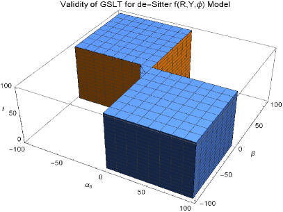
Figure 1: Validity region of the GSLT for de-Sitter $f(R,Y,\phi)$ model with $\alpha_{1}=1$ and $\alpha_{2}=3$.

• de-Sitter model independent of Y

Now we are considering a function $f(R,\phi)$ independent of $Y$ and the model constructed in [43] is defined as

$$f(R,\phi)=\alpha_{1}\alpha_{2}e^{\alpha_{1}R}\phi^{\gamma_{1}}+\gamma_{2}\phi^{\gamma_{3}}+\gamma_{4}\phi^{\gamma_{5}}\,,$$ (38)

where $\alpha_{i}^{\prime}s$ are constants of integration and

$$\gamma_{1} = -\frac{1}{\beta}\Big{(}1+\frac{1}{6H_{0}^{2}\alpha_{1}}\Big{)},~{}~{}\gamma_{2}=\omega_{0}\beta^{2}H_{0}^{2}\,,$$

$$\gamma_{3} = m+2,~{}~{}\gamma_{4}=-2\kappa^{2}\rho_{0}a_{0}^{3(1+w)},~{}~{}\gamma_{5}=-\frac{3}{\beta}\,.$$

Inserting this model in (33), the viability of the GSLT is given by

$$\dot{S}_{tot}=\frac{2\pi}{Gb}\bigg{[}-12kH_{0}(b-1)\alpha_{1}^{3}\alpha_{2}a_{0}^{\beta\gamma_{1}}e^{\alpha_{1}R}e^{-2H_{0}t}e^{\beta\gamma_{1}H_{0}t}+\beta H_{0}(b-1)\alpha_{1}^{2}\alpha_{2}$$

$$\times\gamma_{1}\left(a_{0}^{2}H_{0}^{2}+ke^{-2H_{0}t}\right)a_{0}^{2}a_{0}^{\beta\gamma_{1}}e^{\alpha_{1}R}e^{\beta\gamma_{1}H_{0}t}-2kH_{0}(b-1)\alpha_{1}^{2}\alpha_{2}a_{0}^{2}a_{0}^{\beta\gamma_{1}}e^{\alpha_{1}R}$$

$$\times e^{\beta\gamma_{1}H_{0}t}e^{-2H_{0}t}+2k^{2}H_{0}a_{0}^{2}e^{-4H_{0}t}\left(\frac{b}{2}-1\right)\left(H_{0}^{2}a_{0}^{2}+ke^{-2H_{0}t}\right)^{-1}\alpha_{1}^{2}\alpha_{2}e^{\alpha_{1}R}$$

$$\times e^{\beta\gamma_{1}H_{0}t}a_{0}^{\beta\gamma_{1}}\bigg{]}\left(a_{0}^{2}H_{0}^{2}+ke^{-2H_{0}t}\right)^{-1}\left(2a_{0}^{2}H_{0}^{2}+ke^{-2H_{0}t}\right)^{-1}\geq 0\,.$$ (39)

The viability of the GSLT in de-Sitter $f(R,\phi)$ depends on four parameters $\alpha_{1}$, $\alpha_{2}$, $\beta$ and $t$. By fixing $\beta$ we will observe the variations of $\alpha_{1}$ and $\alpha_{2}$ where GSLT is valid. For all values of $\beta$ and $t$ we have two cases $(i)$ $\alpha_{1}\leq-0.1$ $\forall$ $\alpha_{2}$ $(ii)$ $\alpha_{1}>0$ with $\alpha_{2}\geq 0$.

4.2 Model constructed from power Law method

Power solutions are very useful to discuss the different phases of cosmic evolution e.g., dark energy, matter and radiation dominated epochs. We are discussing here just one power law solution for $f(R,Y,\phi)$ gravity with a power law scale factor defined as [42, 47]

$$a(t)=a_{0}t^{n},~{}~{}H(t)=\frac{n}{t},~{}~{}R=6n(1-2n)t^{-2}\,,$$ (40)

where $n>1$ shows the accelerating picture of the universe, $0<n<1$ leads to decelerated universe, $n=2/3$ leads to dust dominated era and $n=1/2$ for radiation dominated epoch.

• Power Law model independent of Y

In [43], it was constructed a well-behaved model for $f(R,\phi)$ function, so that now we will concentrate in that specific theory and model to show the validity of the GSLT. For this model, the $f(R,\phi)$ function reads

$$f(R,\phi)=\alpha_{1}\alpha_{2}\phi^{\gamma_{1}}R^{\gamma_{2}}+\gamma_{3}\phi^{\gamma_{4}}+\gamma_{5}\phi^{\gamma_{6}}\,,$$

where $\alpha_{i}$ are integration constants and

$$\gamma_{1} = \frac{\alpha_{1}}{3n-1}+\frac{n-3}{n\beta}-\frac{2(3n-1)^{2}}{n^{2}\beta^{2}\alpha_{1}},~{}~{}~{}\gamma_{2}=\frac{n(n-3)\beta\alpha_{1}}{(3n-1)^{2}},$$

$$\gamma_{3} = \omega_{0}\beta^{2}n^{2}a_{0}^{\frac{2}{n}},~{}~{}~{}\gamma_{4}=m+2-\frac{2}{n\beta},~{}~{}~{}\gamma_{5}=-2\kappa\rho_{0}a_{0}^{3(1+w)},~{}~{}~{}\gamma_{6}=-\frac{3}{\beta}.$$

By substituting this model in (33) we get

$$\dot{S}_{tot}=\frac{2\pi}{Gb}\bigg{[}H_{0}(b-1)\alpha_{1}\alpha_{2}\gamma_{2}(\gamma_{2}-1)a_{0}^{\beta\gamma_{1}}t^{n\beta\gamma_{1}}\left(\left(j-q-2\right)H_{0}^{2}+\frac{k}{a_{0}^{2}t^{2n}}\right)$$

$$\times\left((1-q)H_{0}^{2}+\frac{k}{a_{0}^{2}t^{2n}}\right)^{\gamma_{2}-2}+\beta H_{0}\alpha_{1}\alpha_{2}\gamma_{1}\gamma_{2}\left((1-q)H_{0}^{2}+\frac{k}{a_{0}^{2}t^{2n}}\right)^{\gamma_{2}-1}$$

$$\times(b-1)a_{0}^{\beta\gamma_{1}}t^{n\beta\gamma_{1}}-2H_{0}(b-1)\alpha_{1}\alpha_{2}\gamma_{2}a_{0}^{\beta\gamma_{1}}t^{n\beta\gamma_{1}}\left((1-q)H_{0}^{2}+\frac{k}{a_{0}^{2}t^{2n}}\right)^{\gamma_{2}-1}$$

$$\times\left\{1+\frac{qH_{0}^{2}}{H_{0}^{2}+\frac{k}{a_{0}^{2}t^{2n}}}\right\}+2H_{0}\alpha_{1}\alpha_{2}\gamma_{2}a_{0}^{\beta\gamma_{1}}t^{n\beta\gamma_{1}}\left((1-q)H_{0}^{2}+\frac{k}{a_{0}^{2}t^{2n}}\right)^{\gamma_{2}-1}$$

$$\times\left(\frac{b}{2}-1\right)\left(1+\frac{qH_{0}^{2}}{H_{0}^{2}+\frac{k}{a_{0}^{2}t^{2n}}}\right)^{2}\bigg{]}\left((1-q)H_{0}^{2}+\frac{k}{a_{0}^{2}t^{2n}}\right)^{-1}\geq 0.$$ (41)

The above constraint has five parameters $\alpha_{1}$, $\alpha_{2}$, $n$, $\beta$ and $t$. Now, we will check the validity of $\dot{S}_{tot}\geq 0$ for different values of $n$, $\beta$ and $t$ by fixing $\alpha_{1}$, $\alpha_{2}$. All possible cases of this model are written in Table 1.

Let us start with the case $\alpha_{1}>0$ and check the viable ranges of $\alpha_{2}$, $\beta$ and $t$. In this case we have three cases depending on the choice $\alpha_{2}$,

$(i)$ $\alpha_{2}<0$, $n\geq 3$ with ($\beta\leq-35.8$, $t\geq 1$) or ($\beta\geq 2.81$, $t\geq 0.94$).
$(ii)$ $\alpha_{2}=0$, $n>1$ and $\forall$ $t$ with $\beta>0$ or $\beta<0$.
$(iii)$ $\alpha_{2}>0$ with ($n\geq 8.6$, $0<\beta\leq 20$, $t\geq 0.8$) or ($n\geq 12.7$, $-20\leq\beta<0$, $t\geq 0.9$).

If we take $\alpha_{1}<0$ we also have three possible cases where the GSLT will hold,

$(i)$ $\alpha_{2}<0$ with ($n\geq 8.6$, $-20\leq\beta<0$, $t\geq 0.8$) or ($n\geq 12.7$, $0<\beta\leq 20$, $t\geq 0.9$).
$(ii)$ $\alpha_{2}=0$, $n>1$ and $\forall$ $t$ with $\beta>0$ or $\beta<0$.
$(iii)$ $\alpha_{2}>0$, $n\geq 3$ and $\forall$ $t$ with ($\beta\leq-28.1$) or ($\beta\geq 35.7$).

It can be noted that by taking $\alpha_{1}$ and $\alpha_{2}$ with the same sign, $\dot{S}_{tot}\geq 0$ is not valid for initial values of $t$ and $n$, and also that $\beta$ is restricted to $\beta\leq 20$ or $\beta\geq-20$. Fig. (2) depicts the validity region of the GSLT for a specific case in this model, where $\alpha_{1}>0$ and $\alpha_{2}=5$ .

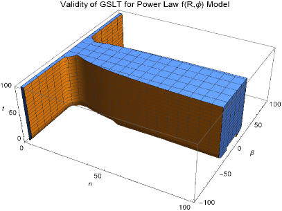
Figure 2: Valdity of the GSLT for Power law-$f(R,\phi)$ versus the parameters $n$, $\beta$ and $t$ with $\alpha_{1}=1$ and $\alpha_{2}=5$.

4.3 $f(R,\phi)$ Models

In this section, we will study the validity of the GSLT using well known forms of $f(R,\phi)$ gravity.

4.3.1 Model-I

Myrzakulov et al. [44] have examined the spectral index and tensor-to-scalar ratio to describe the inflation in $f(R,\phi)$ theories and observed the results using the recent observational data. This model is based on the following function,

$$f(R,\phi)=\frac{R-2\Lambda(1-e^{B\phi\kappa^{3}R})}{\kappa^{2}}\,,$$

where $\kappa^{3}$ is introduced for dimensional reasons and $B$ is a constant. Inserting the model in (33), the inequality becomes

$$\dot{S}_{tot}=\frac{2\pi}{Gb}\bigg{[}2H_{0}(b-1)\Lambda B^{2}a_{0}^{2\beta}t^{2n\beta}\kappa^{4}Re^{Ba_{0}^{\beta}t^{n\beta}\kappa^{3}R}+2\Lambda B\kappa(b-1)\beta H_{0}a_{0}^{\beta}t^{n\beta}$$

$$\times\left(1+Ba_{0}^{\beta}t^{n\beta}\kappa^{3}R\right)e^{Ba_{0}^{\beta}t^{n\beta}\kappa^{3}R}-\frac{2}{\kappa^{2}}H_{0}(b-1)\left\{1+2\Lambda Ba_{0}^{\beta}t^{n\beta}\kappa^{3}e^{Ba_{0}^{\beta}t^{n\beta}\kappa^{3}R}\right\}$$

$$\times\left(1+\frac{qH_{0}^{2}}{H_{0}^{2}+\frac{k}{a_{0}^{2}t^{2n}}}\right)+\frac{2H}{\kappa^{2}}\left(\frac{b}{2}-1\right)\left\{1+2\Lambda Ba_{0}^{\beta}t^{n\beta}\kappa^{3}e^{Ba_{0}^{\beta}t^{n\beta}\kappa^{3}R}\right\}$$

$$\times\left(1+\frac{qH_{0}^{2}}{H_{0}^{2}+\frac{k}{a_{0}^{2}t^{2n}}}\right)^{2}\bigg{]}\left(H_{0}^{2}(1-q)+\frac{k}{a_{0}^{2}t^{2n}}\right)^{-1}\geq 0\,,$$ (42)

where $R=6[(1-q)H_{0}^{2}+k/(a_{0}^{2}t^{2n})]$. As we can notice, the inequality depends on four parameters $B$, $n$, $\beta$ and $t$. We can see that $\dot{S}_{tot}\geq 0$ is satisfied for two cases depending on the choice of $B$:

$(i)$ $B=0$ with $n>1$ and $t\geq 0.96$ (for all values of $\beta$).
$(ii)$ $B>0$ with $n>1$, $\beta\leq-0.6$ and $\forall$ $t$ and $n\geq 2.5$, $\beta\geq 6$ and $t\geq 2.5$.

4.3.2 Model-II

Now, we will explore a model studied in [42], where they considered a function form $f(R,\phi)=Rf(\phi)$ with $\omega(\phi)=\omega_{0}\phi^{m}$ and $\phi=a(t)^{\beta}$. Therefore, we will consider the following function

$$f(R,\phi)=R\left(\frac{\omega_{0}\beta^{2}n^{2}a_{0}^{2/n}(mn\beta+2n\beta+6n-2)}{mn\beta+2n\beta-2}\right)\phi^{m+2-\frac{2}{n\beta}}\,,$$

where $\omega_{0}$ and $a_{0}$ are constants. Introducing this model in (33) we find the constraint

$$\dot{S}_{tot}=\frac{2\pi}{Gb}\bigg{[}\beta^{2}H_{0}(b-1)\omega_{0}n\left(mn\beta+2n\beta+6n-2\right)a_{0}^{\beta(m+2)}t^{mn\beta+2n\beta-2}$$

$$-2H_{0}(b-1)\left(\frac{\omega_{0}\beta^{2}n^{2}a_{0}^{2/n}\left(mn\beta+2n\beta+6n-2\right)}{mn\beta+2n\beta-2}\right)a_{0}^{\beta\left(m+2-\frac{2}{n\beta}\right)}t^{mn\beta+2n\beta-2}$$

$$\times\left\{1+qH_{0}^{2}(H_{0}^{2}+\frac{k}{a_{0}^{2}}t^{2n})^{-1}\right\}+2\left(\frac{b}{2}-1\right)H_{0}a_{0}^{\beta\left(m+2-\frac{2}{n\beta}\right)}t^{mn\beta+2n\beta-2}$$

$$\times\left(\frac{\omega_{0}\beta^{2}n^{2}a_{0}^{2/n}\left(mn\beta+2n\beta+6n-2\right)}{mn\beta+2n\beta-2}\right)\left(1+\frac{qH_{0}^{2}}{H_{0}^{2}+\frac{k}{a_{0}^{2}t^{2n}}}\right)^{2}\bigg{]}$$

$$\times\left(H_{0}^{2}(1-q)+\frac{k}{a_{0}^{2}t^{2n}}\right)^{-1}\geq 0.$$ (43)

One can see that the inequality of this model is depending on four parameters $\beta$, $m$, $n$ and $t$ and hence we will discuss its viability for different values of $\beta$ and $m$ by fixing $n$. For $n>1$ at every time $t$ we have two cases where the validity of the GSLT holds: $m\geq 2$ with $\beta\leq-1.5$ and $m\leq-3.2$ with $\beta\geq 5$. In Fig. 3, the validity of the GSLT region is showed for the parameters $m$, $\beta$ and $t$ by fixing $n>1$.

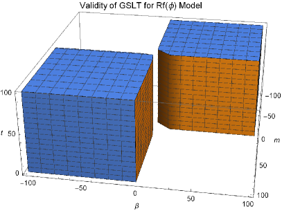
Figure 3: Regions where the GSLT is satisfied for the Model-II versus the parameters $m$, $\beta$ and $t$ with $n=1.1$.

4.3.3 Model-III

Now, we will study the model which is applied to describe the cosmological perturbations for non-minimally coupled scalar field dark energy in both metric and Palatini formalisms [45].

$$f(R,\phi)=R(1+\xi\kappa^{2}\phi^{2}),$$

where $\xi$ is the coupling constant. Using this model in (33) we have

$$\dot{S}_{tot}=\frac{2\pi}{Gb}\bigg{[}2\beta H_{0}\xi\kappa^{2}(b-1)a_{0}^{2\beta}t^{2n\beta}-2H_{0}(b-1)\left(1+\xi\kappa^{2}a_{0}^{2\beta}t^{2n\beta}\right)\times$$

$$\left\{1+qH_{0}^{2}\left(H_{0}^{2}+\frac{k}{a_{0}^{2}}t^{2n}\right)^{-1}\right\}+2\left(\frac{b}{2}-1\right)H_{0}\left(1+\xi\kappa^{2}a_{0}^{2\beta}t^{2n\beta}\right)\times$$

$$\left(1+\frac{qH_{0}^{2}}{H_{0}^{2}+\frac{k}{a_{0}^{2}t^{2n}}}\right)^{2}\bigg{]}\times\left(H_{0}^{2}(1-q)+\frac{k}{a_{0}^{2}t^{2n}}\right)^{-1}\geq 0.$$ (44)

Here, we have four parameters $n$, $\xi$, $\beta$ and $t$. Therefore, we can fix $n$ to find the values of $\xi$ and $\beta$ where the GSLT is satisfied. For $n>1$, it is valid for $\beta\leq-3.5$ with (for all values of $\xi$ and $t\geq 4$) and for $\beta\geq 0.15$ with ($\xi\leq 0$ and $t\geq 1$).

4.3.4 Model-IV

In [46], authors used the following model to discuss the inflationary paradigm

$$f(R,\phi)=\phi(R+\alpha R^{2})\,,$$

where $\alpha$ is a constant with suitable dimensions. Here, we are interested to explore the validity of GSLT for the above model. Introducing this model in (33) we have inequality of the form

$$\dot{S}_{tot}=\frac{2\pi}{Gb}\bigg{[}12\alpha H_{0}(b-1)a_{0}^{\beta}t^{n\beta}\left\{(j-q-2)H_{0}^{2}+\frac{k}{a_{0}^{2}t^{2n}}\right\}+\beta H_{0}(b-1)$$

$$\times a_{0}^{\beta}t^{n\beta}\left\{1+12\alpha\left((1-q)H_{0}^{2}+\frac{k}{a_{0}^{2}t^{2n}}\right)\right\}-2H_{0}(b-1)a_{0}^{\beta}t^{n\beta}\bigg{\{}1+12\alpha$$

$$\times\left((1-q)H_{0}^{2}+\frac{k}{a_{0}^{2}t^{2n}}\right)\bigg{\}}\left\{1+qH_{0}^{2}\left(H_{0}^{2}+\frac{k}{a_{0}^{2}t^{2n}}\right)^{-1}\right\}+2\left(\frac{b}{2}-1\right)$$

$$\times H_{0}a_{0}^{\beta}t^{n\beta}\left\{1+12\alpha\left((1-q)H_{0}^{2}+\frac{k}{a_{0}^{2}t^{2n}}\right)\right\}\left(1+\frac{qH_{0}^{2}}{H_{0}^{2}+\frac{k}{a_{0}^{2}t^{2n}}}\right)^{2}\bigg{]}$$

$$\times\left(H_{0}^{2}(1-q)+\frac{k}{a_{0}^{2}t^{2n}}\right)^{-1}\geq 0.$$ (45)

We have four parameters $n$, $\alpha$, $\beta$ and $t$ to constraint to satisfy the above relation. For $n>1$ we have two cases depending on the choice of $\alpha$:

$(i)$ $\alpha<0$ with $\beta\geq 0$ (for all times $t$).
$(ii)$ $\alpha\geq 0$ with $\beta\leq-0.25$ and $t\geq 1$.

In (4) is showed the evolution of the GSLT in this model for a specific choice of the parameter $n=1.1$

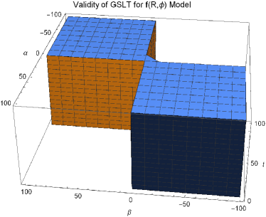
Figure 4: Validity regions of the GSLT for the Model-IV for the parameters $\alpha$ and $\beta$ with $n=1.1$.

5 Equilibrium description of Thermodynamics laws

The reason behind the exists of non-equilibrium term $d_{i}S$ in entropy production is $\rho_{d}$ and $p_{d}$ described in eqs. (12) and (13) satisfy the continuity Eq. (18) whose R.H.S. will not vanish in $f(R,Y,\phi)$ gravity because $\partial_{t}f_{R}\neq 0$. Otherwise the standard continuity equation does not satisfy. Now we are again defining the energy density and pressure of dark components for which the continuity equation holds and no extra entropy production term occur, which is mentioned as the equilibrium description. Here in this section we will examine the equilibrium description of thermodynamics in $f(R,Y,\phi)$ gravity. The field equation (2) is redefined as

$$G_{\mu\nu}+f_{R}R_{\mu\nu}-\frac{1}{2}\left(f+\omega(\phi)\phi_{;\alpha}\phi^{;\alpha}\right)g_{\mu\nu}-f_{R;\mu\nu}+g_{\mu\nu}\Box f_{R}+2f_{Y}R_{\mu}^{\alpha}R_{\alpha\nu}$$

$$-2[f_{Y}R^{\alpha}_{(\mu}]_{;\nu)\alpha}+\Box[f_{Y}R_{\mu\nu}]+[f_{Y}R_{\alpha\beta}]^{;\alpha\beta}g_{\mu\nu}+\omega(\phi)\phi_{;\mu}\phi_{;\nu}=G_{\mu\nu}+\kappa T_{\mu\nu}^{(m)},$$ (46)

where $\Box=g^{\mu\nu}\nabla_{\mu}\nabla_{\nu}$, $f_{R}=\partial f/\partial R$ and $f_{Y}=\partial f/\partial Y$. The energy-momentum tensor for a perfect fluid is defined as

$$T_{\mu\nu}^{(m)}=(\rho_{m}+p_{m})u_{\mu}u_{\nu}+p_{m}g_{\mu\nu},$$ (47)

where $p_{m}$, $\rho_{m}$ and $u_{\mu}$ are the pressure, energy density and the four velocity of the fluid respectively. Hereafter, we will assume that the matter of the universe has zero pressure $p_{m}=0$ (dust). The Einstein field equation from Eq. (5) can be written as

$$R_{\mu\nu}-\frac{1}{2}Rg_{\mu\nu}=8\pi GT_{\mu\nu}^{(m)}+T_{\mu\nu}^{(d)},$$ (48)

where

$$T_{\mu\nu}^{(d)} = -\frac{1}{2}Rg_{\mu\nu}f_{R}+\frac{1}{2}\left(f+\omega(\phi)\phi_{;\alpha}\phi^{;\alpha}\right)g_{\mu\nu}+f_{R}{}_{;\mu\nu}-g_{\mu\nu}\Box f_{R}-2f_{Y}$$ (49)

$$\times R_{\mu}^{\alpha}R_{\alpha\nu}+2[f_{Y}R^{\alpha}_{(\mu}]_{;\nu)\alpha}-\Box[f_{Y}R_{\mu\nu}]-[f_{Y}R_{\alpha\beta}]^{;\alpha\beta}g_{\mu\nu}-\omega(\phi)\phi_{;\mu}\phi_{;\nu}$$

$$+ \left(1-f_{R}\right)G_{\mu\nu},$$

represents an effective energy-momentum tensor related with all the new terms of the theory.

5.1 First Law of Thermodynamics

We are redefining (10) and (11) in the form

$$3\left(H^{2}+\frac{k}{a^{2}}\right) = 8\pi G(\rho_{m}+\rho_{d})\,,$$ (50)

$$-2\left(\dot{H}-\frac{k}{a^{2}}\right) = 8\pi G(\rho_{m}+\rho_{d}+p_{d})\,,$$ (51)

where $\rho_{d}$ and $p_{d}$ are the energy density and pressure of dark components redefined as

$$\rho_{d} = \frac{1}{8\pi G}\bigg{[}\frac{1}{2}\left(Rf_{R}-f\right)-\frac{1}{2}\omega(\phi)\dot{\phi}^{2}-3H\partial_{t}f_{R}-6H\big{(}2\dot{H}+3H^{2}+\frac{k}{a^{2}}\big{)}\partial_{t}f_{Y}$$

$$- f_{Y}\bigg{(}\dddot{H}+4H\ddot{H}+6\dot{H}H^{2}-2H^{4}-\frac{4kH^{2}}{a^{2}}\bigg{)}+3\left(1-f_{R}\right)\left(H^{2}+\frac{k}{a^{2}}\right)\bigg{]}\,,$$

$$p_{d} = \frac{1}{8\pi G}\bigg{[}\frac{1}{2}\left(f-Rf_{R}\right)-\frac{1}{2}\omega(\phi)\dot{\phi}^{2}+\partial_{tt}f_{R}+2H\partial_{t}f_{R}+\left(4\dot{H}+6H^{2}\right.$$ (53)

$$+ \left.\frac{2k}{a^{2}}\right)\partial_{tt}f_{Y}+4H\bigg{(}\dot{H}+3H^{2}+\frac{2k}{a^{2}}\bigg{)}\partial_{t}f_{Y}+f_{Y}\bigg{(}4\dddot{H}+20H\ddot{H}$$

$$+ 10\dot{H}H^{2}+16\dot{H}^{2}-18H^{4}-\frac{18k\dot{H}}{a^{2}}-\frac{20kH^{2}}{a^{2}}-\frac{8k^{2}}{a^{4}}\bigg{)}-\left(1-f_{R}\right)$$

$$\times \left(2\dot{H}+3H^{2}+\frac{k}{a^{2}}\right)\bigg{]}\,.$$

In this representation, eq. (19) becomes

$$d\tilde{r}_{A}=4\pi GH\tilde{r}_{A}^{3}(\hat{\rho}_{\rm total}+\hat{p}_{\rm total})dt\,,$$ (54)

by using the horizon entropy $\hat{S_{h}}$ of the form

$$\hat{S_{h}}=\frac{A}{4G}\,,$$ (55)

differentiating Eq. (55) and using (54), we have

$$\frac{1}{2\pi\tilde{r}_{A}}d\hat{S_{h}}=4\pi\tilde{r}_{A}^{3}\left(\hat{\rho}_{\rm total}+\hat{p}_{\rm total}\right)Hdt\,,$$ (56)

multiplying both sides of the above equation by $1-\dot{\tilde{r}}_{A}/(2H\tilde{r}_{A})$, we have

$$T_{h}d\hat{S_{h}}=-4\pi\tilde{r}_{A}^{3}\left(\hat{\rho}_{\rm total}+\hat{p}_{\rm total}\right)Hdt+2\pi\tilde{r}_{A}^{2}\left(\hat{\rho}_{\rm total}+\hat{p}_{\rm total}\right)d\tilde{r}_{A}\,.$$ (57)

By defining the Misner-Sharp energy as

$$\hat{E}=\frac{\tilde{r}_{A}}{2G}=V\hat{\rho}_{\rm total}\,,$$ (58)

we get

$$d\hat{E}=4\pi\tilde{r}_{A}^{2}\hat{\rho}_{\rm total}d\tilde{r}_{A}-4\pi\tilde{r}_{A}^{3}\left(\hat{\rho}_{\rm total}+\hat{p}_{\rm total}\right)Hdt\,.$$ (59)

Using Eq. (59) in (57), we get

$$T_{h}d\hat{S}_{h}=d\hat{E}-\hat{W}dV\,,$$ (60)

where we have used the work density $\hat{W}=(1/2)(\hat{\rho}_{\rm total}-\hat{p}_{\rm total})$ [37]. The equilibrium description of thermodynamics can be derived by redefining the energy density $\rho_{d}$ and the pressure $p_{d}$ to satisfy the continuity equation.

5.2 Generalized Second Law of Thermodynamics

To analyze the equilibrium description of second law of thermodynamics, we can write the Gibbs equation in terms of all matter and dark energy fluid as

$$T_{\nu}d\hat{S_{\nu}}=d(\hat{\rho}_{\rm total}V)+\hat{p}_{\rm total}dV\,,$$ (61)

where $T_{\nu}$ denotes the temperature within the horizon. The second law of thermodynamics can expressed as

$$\dot{\hat{S_{h}}}+\dot{\hat{S}}_{\nu}\geq 0\,,$$ (62)

where $\hat{S_{h}}$, $\hat{S}_{\nu}$ are the horizon entropy and the entropy due to energy sources inside the horizon respectively. Now, we will assume a relation between the temperature within the horizon and the temperature of the apparent horizon given by

$$T_{\nu}=T_{h}\,.$$ (63)

By substituting Eqs. (60) and (61) in Eq. (62), we obtain

$$\dot{S}_{tot}=\dot{\hat{S_{h}}}+\dot{\hat{S_{\nu}}}=\frac{2\pi\Sigma}{\tilde{r}_{A}R}\geq 0\,,$$ (64)

where

$$\Sigma=\frac{1}{2}(\hat{\rho}_{\rm total}+\hat{p}_{\rm total})\dot{V}\,,$$

which is the general condition to satisfy the GSLT. Using Eqs. (50) and (51), the condition (64) reduced to

$$\frac{2\pi H\left(\frac{2k\dot{H}}{a^{2}}-\dot{H}^{2}-\frac{k^{2}}{a^{4}}\right)}{G\left(\dot{H}+2H^{2}+\frac{k}{a^{2}}\right)\left(H^{2}+\frac{k}{a^{2}}\right)^{2}}\geq 0,$$ (65)

In case of flat FRW universe to protect the GSLT, the condition (65) must be satisfied.

6 Conclusions

Scalar tensor theories of gravity appeared as one of the significant representation in the bunch of alternatives theories of gravity. These theories proved to be much promising due to their vast applications in gravitation and cosmology. These theories play key role in developing models of inflation and DE. In the present paper, we have discussed the thermodynamical laws in the context of modified $f(R,R_{\mu\nu}R^{\mu\nu},\phi)$ theory, which involves the Ricci scalar, the contraction of the Ricci tensor $Y=R_{\mu\nu}R^{\mu\nu}$ (Ricci invariant) and a scalar field $\phi$. This theory can be regarded as an extended form of $f(R,\phi)$ gravity. Here, we have presented the general formalism of field equations for FRW spacetime with any spatial curvature in this theory and shown that these equations can be cast to the form of FLT $T_{h}d\hat{S}_{h}+T_{in}d\hat{S}_{in}=\delta{Q}$, in non-equilibrium and $T_{h}d\hat{S}_{h}=\delta{Q}$ in equilibrium description of thermodynamics. In this structure of FLT we find that entropy is contributed from two factors, first one corresponds to horizon entropy defined in terms of area and second represents the entropy production term $d\bar{S}$ which is produced because of the non-equilibrium description in $f(R,Y,\phi)$ gravity. It is worth mentioning that no such term is present in Einstein, Gauss-Bonnet, scalar-tensor theory with non-minimally derivative coupling, Lovelock and braneworld modified theories [17]-[22]. However, in case of modified theories like $f(R)$ and scalar tensor theories people have suggested various schemes to avoid the additional entropy term in first law of thermodynamics [49, 24, 25]. Following such approach one can also discuss the equilibrium thermodynamics as done in [30].

Moreover, the validity of GSLT at the apparent horizon of FRW universe is also tested in this modified theory. We present the general relation involving contributions from horizon entropy, auxiliary entropy terms and associated with the matter contents within the horizon is presented in comprehensive way. Here, we have assumed the proportionality relation between the temperatures related to apparent horizon and matter components inside the horizon. To discuss the validity of GSLT, we have selected the more generic models reconstructed in [43], where we consider the de Sitter and power law cosmological backgrounds. The discussion are indetail as we have also considered some well known models from different backgrounds to validate the GSLT. We can retrieve the results in other modified theories depending on the choice of the Lagrangian $f(R,Y,\phi)$. When we consider function independent of $Y$ we can reduce the results of $f(R,Y,\phi)$ into $f(R,\phi)$ gravity and choosing $f(R,Y,\phi)=R\phi$ we get the results for Brans-Dick theory. Further, by considering a function independent of $Y$ and $\phi$ we get the results for $f(R)$ gravity. Table 1 summarizes the regions where the GSLT is satisfied for all the models that we discussed in this paper.

In a de-Sitter $f(R,Y,\phi)$ model, one can notice that the validity of the GSLT depends on five parameters $\alpha_{1}$, $\alpha_{2}$, $\alpha_{3}$, $\beta$ and $t$ and hence we fixed two parameters, $\alpha_{1}$ and $\alpha_{2}$ to show the viable regions by varying the other parameters. Next we have considered $f(R,\phi)$ using de-Sitter model whose GSLT constraint depends on four parameters $\alpha_{1}$, $\alpha_{2}$, $\beta$ and $t$. Here we are fixing $\beta$ and observe the feasible regions by varying the other parameters. In power law $f(R,\phi)$ case by varying $\alpha_{1}$, $\alpha_{2}$ we have examined the feasible constraints on $\beta$, $n$ and $t$. Next we have considered four known models of $f(R,Y,\phi)$ gravity independent of $Y$, which are of the form $f(R,\phi)$, $Rf(\phi)$, $\phi f(R)$. Model-I is depending on four parameters $B$, $n$, $\beta$ and $t$, we have checked the validity of $\dot{S}_{tot}\geq 0$ by varying $B$. Model-II is a function of four parameters $\beta$, $m$, $n$ and $t$, by fixing $n$ we will discuss the viability of the GSLT for different values of $\beta$, $m$ and $t$. In model-III the constraint is depending on four parameters $n$, $\xi$, $\beta$ and $t$. By fixing $n>1$ we examined the possible regions for the other parameters. Next in model-IV we have four parameters $n$, $\alpha$, $\beta$ and $t$. For $n>1$ we have find the feasible constraints on other parameters.

Models	Variations of parameters	Validity of $\dot{S}_{tot}\geq 0$
	$\alpha_{1}>0$, $\alpha_{2}>0$ and	$\forall$ $t$ with ($\alpha_{3}\geq 0$, $\beta\leq-0.78$) or ($\alpha_{3}\leq 0$, $\beta\geq 0$)
de-Sitter Model	$\alpha_{1}<0$, $\alpha_{2}>0$
$f(R,Y,\phi)$	$\alpha_{1}>0$, $\alpha_{2}<0$ and	$\forall$ $\alpha_{3}$, $\beta$ and $t$
	$\alpha_{1}<0$, $\alpha_{2}<0$
de-Sitter Model $f(R,\phi)$	$\forall$ $\beta$	$\forall$ $t$ with ($\alpha_{1}\leq-0.1$, $\forall$ $\alpha_{2}$) or ($\alpha_{1}>0$, $\alpha_{2}\geq 0$)
	$\alpha_{1}>0$ with $\alpha_{2}<0$	$n\geq 3$ with ($\beta\leq-35.8$, $t\geq 1$) or ($\beta\geq 2.81$, $t\geq 0.94$)
	$\alpha_{2}=0$	$n>1$, $\beta>0$ or $\beta<0$, $\forall$ $t$
Power Law Model	$\alpha_{2}>0$	($n\geq 8.6$, $0<\beta\leq 20$, $t\geq 0.8$) or ($n\geq 12.7$, $-20\leq\beta<0$, $t\geq 0.9$)
$f(R,\phi)$	$\alpha_{1}<0$ with $\alpha_{2}<0$	($n\geq 8.6$, $-20\leq\beta<0$, $t\geq 0.8$) or ($n\geq 12.7$, $0<\beta\leq 20$, $t\geq 0.9$)
	$\alpha_{2}=0$	$n>1$, $\beta>0$ or $\beta<0$, $\forall$ $t$
	$\alpha_{2}>0$	$n\geq 3$ and $\forall$ $t$ with ($\beta\leq-28.1$) or ($\beta\geq 35.7$)
	$B=0$	$n>1$, $\forall$ $\beta$, $t\geq 0.96$
Model-I	$B>0$	($n>1$ with $\beta\leq-0.6$, $\forall$ $t$) or ($n\geq 2.5$ with $\beta\geq 6$, $t\geq 2.5$)
	$B<0$	not valid
Model-II	$n>1$	$\forall$ $t$ with ($m\geq 2$, $\beta\leq-1.5$) or ($m\leq-3.2$, $\beta\geq 5$)
Model-III	$n>1$	($\forall$ $\xi$, $\beta\leq-3.5$ and $t\geq 4$) or ($\xi\leq 0$, $\beta\geq 0.15$ and $t\geq 1$)
Model-IV	$n>1$	($\beta\geq 0$, $\alpha<0$ and $\forall$ $t$) or ($\beta\leq-0.25$, $\alpha\geq 0$ and $t\geq 1$)

Table 1: Validity regions of $\dot{S}_{tot}\geq 0$ for different models.

7 Acknowledgment

S.B. is supported by the Comisión Nacional de Investigación Científica y Tecnológica (Becas Chile Grant No. 72150066).

References

- [1] Jain, B and Taylor, A.: Phys. Rev. Lett. 91 (2003) 141302.
- [2] Seljak, U. et al.: Phys. Rev. D71 (2005) 103515.
- [3] Komatsu, E. et al.: Astrophys.J. Suppl. 180 (2009) 330.
- [4] Komatsu, E. et al.: Astrophys. J. Suppl. 192 (2011) 18.
- [5] Perlmutter, S. et al.: Astrophys. J. 517 (1999) 565.
- [6] Eisenstein, D. J. et al.: Astrophys. J. 633 (2005) 560.
- [7] Copeland, E.J., Sami, M. and Tsujikawa, S.: Int. J. Mod. Phys. D 15 (2006) 1753.
- [8] Li, M. et al.: Commun. Theor. Phys. 56 (2011) 525.
- [9] Hawking, S.W.: Commun. Math. Phys. 43 (1975) 199.
- [10] Bardeen, J.M., Carter, B., and Hawking, S.: Commun. Math. Phys. 31 (1973) 161.
- [11] Bekenstein, J.D.: Phys. Rev. D 7 (1973) 2333.
- [12] Jacobson, T.: Phys. Rev. Lett. 75 (1995) 1260.
- [13] E. Verlinde, hep-th/0008140.
- [14] Padmanabhan, T.: Phys. Rep. 406 (2005) 49.
- [15] Padmanabhan, T.: Class. Quantum Grav. 19(2002)5387.
- [16] Paranjape, A., Sarkar, S. and Padmanabhan, T.:Phys. Rev. D 74(2006)104015; Kothawala, D. and Padmanabhan, T.: Phys. Rev. D 79(2009)104020.
- [17] Cai, R. G. and Kim, S. P.: JHEP. 02 (2005) 050.
- [18] Akbar, M. and Cai, R. G.: Phys. Lett. B 635 (2006) 7.
- [19] Sadjadi, H. M.: Phy. Rev. D 73 (2006) 063525.
- [20] Sadjadi, H. M.: Phy. Rev. D 76 (2007) 104024.
- [21] Akbar, M.: Chin. Phys. Lett. 25 (2008) 4199.
- [22] Jamil, et al.: JCAP 11(2010)032; Phys. Review D 81, 023007 (2010).
- [23] Cembranos, J.A.R., de la Cruz-Dombriz, A. and Jarillo, J.: Universe 1 (2015) no.3, 412-421; Cembranos, J.A.R., A. de la Cruz-Dombriz and Jarillo J. JCAP 1502 (2015) no.02, 042; J.A.R. Cembranos, A. de la Cruz-Dombriz, P. Jimeno Romero; Int.J.Geom.Meth.Mod.Phys. 11 (2014) 1450001; A. de la Cruz-Dombriz, A. Dobado, A.L. Maroto Published in Phys.Rev. D80 (2009) 124011.
- [24] Bamba, K. and Geng, C. Q.: JCAP. 06 (2010) 014.
- [25] Bamba, K. and Genga, C.Q.: JCAP. 11 (2011) 008.
- [26] Wu, Y.B. et al.: Phys. Lett. B 717 (2012) 323.
- [27] Sharif, M. and Zubair, M.: JCAP. 03 (2012)028; J. Exp. Theor. Phys. 117(2013)248; Adv. High Energy Phys. 2013, 947898(2013).
- [28] Zubair, M. and Abdul Jawad: Astrophys. Space Sci. (2015) 360:11; Zubair, M. and Saira Waheed: Astrophys. Space Sci. (2015) 360:68.
- [29] Sharif, M. and Zubair, M.: JCAP. 11 (2013) 042.
- [30] Huang, Y. et al.: Eur. Phys. J. C. 75 (2015) 351; Bamba, K. and Geng, C. Q: JCAP. 06 (2010) 014.
- [31] Faraoni, V.: Entropy 2010, 12, 1246-1263; Setare, M.R.: Phys. Lett. B 641 (2006) 130133; Huang, Y. et al.: Eur. Phys. J. C. 75(2015)351; Das, S. et al.: Eur. Phys. J. C (2015) 75:504; Akbar, M. and Cai, R. G.: Phys. Lett. B 635 (2006) 7; Sharif, M. and Waheed, S.: Astrophys. Space Sci. 346 (2013) 583-597.
- [32] Lambiase, G. et al.: JCAP. 07 (2015) 003.
- [33] Wald, R. M.: Phys. Rev. D 48 (1993) 3427.
- [34] Brustein, R., Gorbonos, D. and Hadad, M.: Phys. Rev. D 79 (2009) 044025.
-
[35]
Misner, C. W. and Sharp, D. H.: Phys. Rev. 136
(1964) B571;
Bak, D. and Rey, S.-J.: Class. Quant. Grav. 17 (2000) L83. - [36] Wu, S. F., et al.: Class. Quantum Grav. 25 (2008) 235018.
- [37] Hayward, S. A.: Class. Quant. Grav. 15 (1998) 3147; Hayward, S.A., Mukohyama, S. and Ashworth, M.: Phys. Lett. A 256 (1999) 347.
- [38] Bamba, K. and Geng, C. Q.: Phys. Lett. B 679 (2009) 282.
- [39] M. Zubair and S. Bahamonde, arXiv:1604.02996 [gr-qc].
- [40] Izquierdo, G. and Pavon, D.: Phys. Lett. B 633 (2006) 420.
-
[41]
Banerjee, N. and Pavon, D.: Phys. Lett. B
647(2007)477;
Bertolami, O. and Martins, P. J.: Phys Rev D 61(2000)064007. - [42] Ade, P. A. R. et al.: arXiv:1502.01589.
- [43] Zubair, M. and Kouser, F.: Eur. Phys. J. C (to appear 2016).
- [44] Myrzakulov, R., Sebastiani, L. and Vagnozzi, S.: Eur. Phys. J. C 75 (2015) 9,444.
- [45] Fan, Y., Wu, P. and Yu, H.: Phys. Rev. D 92 (2015) 083529.
- [46] Bahamonde, S. et al.: Universe 1 (2015) 2,186.
- [47] Sharif, M. and Zubair, M.: Gen. Relativ. Gravit. 46 (2014)1723; J. Phys. Soc. Jpn. 82 (2013) 014002.
- [48] Akbar, M. and Cai, R.G.: Phys. Rev. D 75(2007)084003; Cai, R.G. and Cao, L.M.: Nucl. Phys. B 785(2007)135; Cai, R.G., Cao, L.M. and HU, Y.P.: JHEP 08(2008)090; Huang, Y. et al.: Eur. Phys. J. C. 75 (2015) 351.
- [49] Gong, Y. and Wang, A.: Phys. Rev. Lett. 99(2007)211301; Wu, S.-F., Ge, X.-H., Zhang, P.-M. and Yang, G.-H.: Phys. Rev. D 81(2010)044034.