Data-Driven Confounder Selection via Markov and Bayesian Networks

Summary: To unbiasedly estimate a causal effect on an outcome unconfoundedness is often assumed. If there is sufficient knowledge on the underlying causal structure then existing confounder selection criteria can be used to select subsets of the observed pretreatment covariates, $X$, sufficient for unconfoundedness, if such subsets exist. Here, estimation of these target subsets is considered when the underlying causal structure is unknown. The proposed method is to model the causal structure by a probabilistic graphical model, e.g., a Markov or Bayesian network, estimate this graph from observed data and select the target subsets given the estimated graph. The approach is evaluated by simulation both in a high-dimensional setting where unconfoundedness holds given $X$ and in a setting where unconfoundedness only holds given subsets of $X$. Several common target subsets are investigated and the selected subsets are compared with respect to accuracy in estimating the average causal effect. The proposed method is implemented with existing software that can easily handle high-dimensional data, in terms of large samples and large number of covariates. The results from the simulation study show that, if unconfoundedness holds given $X$, this approach is very successful in selecting the target subsets, outperforming alternative approaches based on random forests and LASSO, and that the subset estimating the target subset containing all causes of outcome yields smallest MSE in the average causal effect estimation. Key words: Bayesian networks; Causal inference; Confounding; Covariate selection; Markov networks; Matching; TMLE.

^∗email: jenny.haggstrom@umu.se

1 Introduction

To get an unbiased estimate of a causal effect, of a treatment on some outcome, the treatment assignment is often assumed to be unconfounded, which is the case, e.g., when assignment to treatment is randomized. In an observational study treatment assignment is not randomized, and to get unbiased causal effect estimates we need to make sure that the assumption of unconfoundedness is plausible when conditioning on some set of covariates. Two important questions are: 1) Which set of covariates should we aim to condition on? and 2) How should we in practice go about to select the latter set of covariates? Often the answer to the first question has been ”the set of covariates that are common causes of treatment and outcome” or ”all observed pretreatment covariates”, hereinafter referred to as ’the common cause criterion’ and ’the pretreatment criterion’, respectively. However, in response to Rubin (2007), in a series of letters to the editor and author’s replies (Shrier, 2008; Rubin, 2008a; Pearl, 2009b; Sjölander, 2009; Rubin, 2009) and later on in VanderWeele and Shpitser (2011) it was discussed under what circumstances conditioning on the covariate set defined by the common cause criterion or the pretreatment criterion will in fact induce bias in the causal effect estimate instead of reducing it.

In an attempt to mediate between the standpoints of Pearl, Shrier, Sjölander and Rubin VanderWeele and Shpitser (2011) proposed an alternative covariate selection criterion, ’the disjunctive cause criterion’. The disjunctive cause criterion entails selecting all covariates that are causes of treatment and/or causes of outcome, and will, under certain assumptions, result in unconfoundedness. Specifically, the disjunctive cause criterion is similar to ’the backdoor path criterion’ (Pearl, 1995) in the sense that the covariate set selected by the disjunctive cause criterion will suffice to block all backdoor paths from treatment to outcome if such a set exists. The main practical difference between these two criteria is that to use the backdoor path criterion, knowledge of the full causal structure of the data is needed but to use the disjunctive cause criterion it is sufficient to know which covariates are causes of the treatment and which covariates are causes of the outcome. VanderWeele and Shpitser (2011) dismiss the practical usefulness of the backdoor path criterion and point out that ”In a number of analyses in the biomedical and social sciences, such complete knowledge of causal structures is unlikely” (Section 1, p.1406). Regarding the knowledge of the causal structure that is required for use of the disjunctive cause criterion, they are however optimistic, stating that ”In many epidemiological and biomedical applications, subject matter experts have intuitive knowledge of whether each covariate is a cause of the treatment or the outcome” (Section 6, p.1411). If it is indeed the case, that we have the knowledge required to use the disjunctive cause criterion (or the backdoor path criterion), then the problem of covariate selection, with respect to unconfoundedness, is solved and the question in 2) is redundant.

However, when knowledge of the causal structure is not sufficient for use of the disjunctive cause criterion the process of covariate selection can be aided by data-driven procedures. Moreover, even in cases where the disjunctive cause criterion can be used, mean squared error of nonparametric estimators of causal effects may be improved by further reducing the dimensionality of the covariate set (de Luna, Waernbaum, and Richardson, 2011). Given a set of covariates such that conditioning on this set unconfoundedness is upheld the latter authors propose general algorithms, in line with the common cause criterion, for selecting minimal sets of covariates such that unconfoundedness still holds when conditioning on the selected sets. These algorithms are implemented using marginal coordinate hypothesis testing (continuous covariates) and kernel smoothing (continuous and/or discrete covariates) in the R package CovSel (Häggström, Persson, Waernbaum, and de Luna, 2015). These implementations have in simulation studies (Persson, Häggström, Waernbaum, and de Luna, 2017) been shown to perform well in reducing the dimensionality of the covariate set while still upholding unconfoundedness, thereby resulting in improved mean squared error. For other recently proposed covariate selection procedures see, e.g., Persson et al. (2017), Schnitzer et al. (2016) and references therein. Existing proposals have in common that they are computer intensive, yielding prohibitive running times in high dimensional applications (in terms of number of covariates and number of units).

In this paper we propose and study the use of Markov and Bayesian network algorithms, more precisely Max-Min Parents and Children (MMPC) and Max-Min Hill-Climbing (MMHC) (Tsamardinos, Brown, and Aliferis, 2006), in conjunction with the covariate selection algorithms in de Luna et al. (2011). MMHC has in empirical evaluations been shown to outperform the PC algorithm (Spirtes et al., 2000), previously studied by Maathuis, Kalisch, and Bühlmann (2009) in a similar causal inference setting (although not for explicitly selecting covariates), both with regard to computation time and in ability to accurately estimate the true causal structure (Tsamardinos et al., 2006). To the author’s knowledge, using estimated graphs to explicitly select covariates to control for, as a step completely separated from the nonparametric estimation of causal effects, has not been proposed and studied elsewhere.

The performance of the proposed data-driven covariate selection procedures is investigated, using simulations, in two general high-dimensional scenarios: 1) Unconfoundedness holds given the full covariate set, 2) Unconfoundedness does not hold given the full covariate set, but it does hold given a subset of the full covariate set. In scenario 1), the results show that this approach is very successful in selecting the target covariate subsets. Furthermore, targeting the subset containing all causes of outcome often yields smallest MSE in the average causal effect (ACE) estimation, but the magnitude of the reduction in MSE (relative to conditioning on the full covariate set) depends on the ACE estimator. The proposed covariate selection algorithms are implemented in the R package CovSelHigh (Häggström, 2016).

The remainder of this paper is organized as follows. In Section 2 relevant notation and concepts from causal inference are reviewed. Section 3 focuses on covariate selection when the causal structure is known and Section 4 on covariate selection using Markov and Bayesian network algorithms when the causal structure is unknown. In Section 5 the simulation study is presented. In Section 6 the proposed approach is illustrated using a large register data set with which the ACE of C-section delivery on asthma medication early in life is estimated. The paper is concluded with a discussion in Section 7.

2 Context and Terminology

2.1 Potential Outcomes and Unconfoundedness

Let $T$ denote a binary treatment, $Y$ denote outcome and $X$ denote the set of observed pretreatment covariates, i.e., the full covariate set. Within the potential outcome framework (Neyman, 1923; Rubin, 1974) we let $Y(1)$ and $Y(0)$ denote the potential outcomes for $Y$ under the two treatments $T=1$ and $T=0$, respectively. Since only one treatment assignment is possible for each unit only one of the two potential outcomes is observed, $Y=Y(0)(1-T)+Y(1)T$. In this paper, the ACE, $\beta=E\{Y(1)-Y(0)\}$, is the parameter of interest.

If treatment assignment is not randomized, $\beta$ is identified if a unit’s potential outcomes does not depend on the treatments received by other units (stable unit treatment assumption, SUTVA) (Rubin, 1990) and we have available a set of pretreatment covariates $S$ such that the probability of receiving either treatment conditional on $S$ is bounded away from 0 (overlap assumption) and such that the treatment assignment is unconfounded conditional on $S$. Letting $\perp\!\!\!\perp$ mean ”is independent of” (Dawid, 1979) the assumption of unconfoundedness is upheld if $Y(1),Y(0)\perp\!\!\!\perp T\mid S.$

2.2 Graphical Models

A graph $G=(V,E)$ consists of a set of vertices $V=\{V_{i}:i\in 1,\ldots,p\}$ and a set of edges $E$. The vertices represent random variables, and the edges describe pairwise relationships among the variables. Here, the two types of graphs considered are undirected graphs and directed acyclic graphs (DAGs). In an undirected graph all edges are undirected (—) and in a directed graph all edges are directed $(\rightarrow)$. A directed graph with no cycles is a DAG. Two vertices are adjacent if they are connected by an edge and the neighbors of a vertex $V_{i}$ consists of all vertices adjacent to $V_{i}$. Furthermore, we define a path in a graph as a sequence of edges connecting vertices such that each vertex on the path is visited only once. In a DAG a vertex is a collider on a path if the path enters and leaves the vertex via arrowheads. In this paper we interpret directed edges as causal, i.e., $V_{1}\rightarrow V_{2}$ means that $V_{1}$ is a cause of $V_{2}$, also $V_{1}$ is said to be a parent of $V_{2}$ and $V_{2}$ the child $V_{1}$ (Pearl, 2009a). In an undirected graph the Markov blanket of a vertex consists of the vertex’s neighbors and in a DAG the Markov blanket of a vertex consists of the vertex’s parents, children and children’s other parents. The local Markov property holds with respect to an undirected graph $G$ if there exists a joint probability distribution for $V$ such that, for each $V_{i}\in V$, $V_{i}$ is conditionally independent of its non-neighbors given its neighbors. For a DAG the local Markov property holds if there exists a joint probability distribution for $V$ such that, for each $V_{i}\in V$, $V_{i}$ is conditionally independent of its non-descendants given its parents.

A Markov network is a model consisting of an undirected graph, $G=(V,E)$, and a joint probability distribution $P$ defined over $V$ such that the local Markov property holds with respect to $G$. Similarly, a Bayesian network is a model consisting of a DAG, $G=(V,E)$, and a joint probability distribution $P$ defined over $V$ such that the local Markov property holds with respect to $G$. A probability distribution is faithful to the graph if it obeys no further conditional independence relations than what are entailed by the local Markov property.

3 Target Covariate Subsets

In this section, target covariate subsets are defined using the languages of potential outcomes and graphical models. Let $G_{t}=(V_{t},E_{t})$ with $V_{t}=\{X,T,Y(t)\}$ for $t=0,1$. The subset of $X$ that includes all causes of treatment is defined as $X_{\rightarrow T}=\{X_{i}\in X:X_{i}\rightarrow T\in E_{0}\cup E_{1}\}$. Similarly, let $X_{\rightarrow Y}=X_{\rightarrow Y}^{0}\cup X_{\rightarrow Y}^{1}=\{X_{i}\in X:X_{i}\rightarrow Y(0)\in E_{0}\}\cup\{X_{i}\in X:X_{i}\rightarrow Y(1)\in E_{1}\}$ be the subset of $X$ that includes all causes of outcome. Furthermore, let the subset of $X_{\rightarrow T}$ consisting of elements dependent with outcome be defined as $Q_{\rightarrow T}=Q_{\rightarrow T}^{0}\cup Q_{\rightarrow T}^{1}$ where $Q_{\rightarrow T}^{t}\subseteq X_{\rightarrow T}$ such that $Y(t)\perp\!\!\!\perp X_{\rightarrow T}\setminus Q_{\rightarrow T}^{t}\mid Q_{\rightarrow T}^{t}$, for $t=0,1$, and let the subset of $X_{\rightarrow Y}$ consisting of elements dependent with treatment be defined as $Z_{\rightarrow Y}=Z_{\rightarrow Y}^{0}\cup Z_{\rightarrow Y}^{1}$ where $Z_{\rightarrow Y}^{t}\subseteq X_{\rightarrow Y}^{t}$ such that $T\perp\!\!\!\perp X_{\rightarrow Y}^{t}\setminus Z_{\rightarrow Y}^{t}\mid Z_{\rightarrow Y}^{t}$, for $t=0,1$. Defined in line with the common cause criterion, $Q_{\rightarrow T}$ is a subset of the covariates that cause treatment, and $Z_{\rightarrow Y}$ a subset of the covariates that cause outcome.

The following, similar but not identical to the above, sets are defined in de Luna et al. (2011): $X_{T}\subseteq X$ such that $T\perp\!\!\!\perp X\setminus X_{T}\mid X_{T}$, $X_{Y}=X_{0}\cup X_{1}$ where $X_{t}\subseteq X$ such that $Y(t)\perp\!\!\!\perp X\setminus X_{t}\mid X_{t}$ for $t=0,1$, $Q_{t}\subseteq X_{T}$ such that $Y(t)\perp\!\!\!\perp X_{T}\setminus Q_{t}\mid Q_{t}$ for $t=0,1$ and $Z_{t}\subseteq X_{Y}$ such that $T\perp\!\!\!\perp X_{Y}\setminus Z_{t}\mid Z_{t}$ for $t=0,1$. As long as we have unconfoundedness given $X$ the following equalities hold: $X_{\rightarrow T}=X_{T}$, $X_{\rightarrow Y}=X_{Y}$, $Q_{\rightarrow T}=Q$ and $Z_{\rightarrow Y}=Z$. The latter authors also state assumptions under which these sets are unique (de Luna et al., 2011, Lemmas A2-A5) and $Z$ and $Q$ are minimal sets that cannot be reduced without violating unconfoundedness (de Luna et al., 2011, Proposition 8). The above equalities do not hold in general since $X_{\rightarrow T}$ and $X_{\rightarrow Y}$ are defined in terms of edges present in a DAG while de Luna et al. (2011) define all sets in terms of conditional independencies.

The subset of $X$ that includes all causes of treatment and/or outcome, i.e., the disjunctive cause criterion subset, is defined as $X_{\rightarrow T,Y}=X_{\rightarrow T}\cup X_{\rightarrow Y}$. VanderWeele and Shpitser (2011) suggest a criterion where covariates unassociated with the outcome are iteratively discarded from $X_{\rightarrow T,Y}$, henceforth ’the disjunctive cause criterion with backward selection’, and the subset of $X_{\rightarrow T,Y}$ consisting of elements that are associated with outcome is defined as $W_{\rightarrow Y}=W_{\rightarrow Y}^{0}\cup W_{\rightarrow Y}^{1}$ where $W_{\rightarrow Y}^{t}\subseteq X_{\rightarrow T,Y}$ such that $Y(t)\perp\!\!\!\perp X_{\rightarrow T,Y}\setminus W_{\rightarrow Y}^{t}\mid W_{\rightarrow Y}^{t}$, for $t=0,1$. If $X_{\rightarrow T}$ and $X_{\rightarrow Y}$ are uniquely defined then it follows that $X_{\rightarrow T,Y}$ is unique and under assumptions similar to Lemma A3 in de Luna et al. (2011) so is $W_{\rightarrow Y}$.

For illustrative purposes consider the causal diagram in Figure 1. Here, the observed pretreatment covariates $X=\{X_{i}:i\in 1,\ldots,10\}$ are the only variables affecting $T$ and $Y$ and thus all of the covariate selection criteria mentioned in Section 1 would result in unconfoundedness. The target sets are $X_{\rightarrow T}=X_{T}=\{X_{1},X_{2},X_{3},X_{4},X_{7}\}$, $X_{\rightarrow Y}=X_{Y}=\{X_{1},X_{2},X_{5},X_{6},X_{8}\}$, $Q_{\rightarrow T}=Q=\{X_{1},X_{2},X_{7}\}$, $Z_{\rightarrow Y}=Z=\{X_{1},X_{2},X_{8}\}$, $X_{\rightarrow T,Y}=\{X_{1},X_{2},X_{3},X_{4},X_{5},X_{6},X_{7},X_{8}\}$ and $W_{\rightarrow Y}=\{X_{1},X_{2},X_{5},X_{6},X_{7},X_{8}\}$.

The common cause criterion would select $S=\{X_{1},X_{2},X_{7}\}=Q_{\rightarrow T}$, the pretreatment criterion would select $S=X$, the backdoor path criterion would select $S=\{X_{1},X_{2},X_{3},X_{4},X_{7}\}$, the disjunctive cause criterion would select $S=X_{\rightarrow T,Y}$ and the disjunctive cause criterion with backward selection would select $S=W_{\rightarrow Y}$.

Figure 1: A causal DAG without unobservables.

Now consider the causal diagram in Figure 2. Here, in addition to $T$, $Y$ and $X=\{X_{i}:i\in 1,\ldots,10\}$ we have a set of unobserved variables $U=\{U_{1},U_{2},U_{3}\}$ affecting $T$ and/or $Y$. The target sets $X_{\rightarrow T}$, $X_{\rightarrow Y}$, $Z_{\rightarrow Y}$, and $X_{\rightarrow T,Y}$ remain as for Figure 1 but now $Q_{\rightarrow T}=\{X_{1},X_{2},X_{4},X_{7}\}$, and $W_{\rightarrow Y}=\{X_{1},X_{2},X_{4},X_{5},X_{6},X_{7},X_{8}\}$.

As pointed out by VanderWeele and Shpitser (2011), in this setting not all of the above covariate selection criteria would result in unconfoundedness. Except for the disjunctive cause criterion with backward selection, all of the criteria would in this setting select the same sets as in the previous setting. However, the set selected by the common cause criterion, $\{X_{1},X_{2},X_{7}\}\neq Q_{\rightarrow T}$, would not result in unconfoundedness since it does not include the covariate $X_{4}$, which is now related to both $T$ and $Y$, the latter through the unobserved variable $U_{3}$. The set selected by the pretreatment criterion would fail to achieve unconfoundedness due to the inclusion of the covariate $X_{9}$, which is now a collider on the path between $T$ and $Y$ due to the unobserved variables $U_{1}$ and $U_{2}$. Conditioning on $X_{9}$ will thus open up this path between $T$ and $Y$ and introduce the so called $M$-bias (Greenland, 2003). The sets selected by the backdoor path criterion and the disjunctive cause criterion would however achieve unconfoundedness since both sets would include $X_{4}$ but not $X_{9}$. The disjunctive cause criterion with backward selection would select $S=\{X_{1},X_{2},X_{4},X_{5},X_{6},X_{7},X_{8}\}=W_{\rightarrow Y}$ which includes $X_{4}$ since it is now associated with the outcome and conditioning on this set upholds unconfoundedness. Conditioning on $Q_{\rightarrow T}$ would also, in this case, result in unconfoundedness.

Note that here the sets defined in de Luna et al. (2011) are $X_{T}=X_{\rightarrow T}\cup\{X_{9}\}$, $X_{Y}=X_{\rightarrow Y}\cup\{X_{4},X_{9}\}$, $Q=Q_{\rightarrow T}\cup\{X_{9}\}$ and $Z=Z_{\rightarrow Y}\cup\{X_{4},X_{9}\}$, all including $X_{9}$.

Figure 2: A causal DAG with unobservables.

4 Covariate Selection When the Causal Structure is Unknown

Given the setup stated in Section 2, and no further knowledge on the causal structure, only the pretreatment criterion can be readily used without aid of data-driven procedures. If we, in some way, from data estimate the dependence structure in the form of an undirected or directed graph then we can use the estimated graph to select covariates by reading off which covariates are related to $T$ and/or $Y\mid T=t$ for $t=0,1$.

There are many different methods available for estimating Markov and Bayesian networks (see, e.g., Friedman et al., 1999; Spirtes et al., 2000; Chickering, 2002; Tsamardinos et al., 2006, and references therein). In this paper, the Max-Min Parents and Children Algorithm (MMPC) and the Max-Min Hill-Climbing Algorithm (MMHC) are used to estimate the underlying structure of the data. Algorithms used for estimating such networks can be classified as either constraint-based or score-based. MMHC is a hybrid algorithm which as a first step uses the constraint-based MMPC algorithm to estimate a Markov network, i.e., an undirected graph, and as a second step uses the score-based local optimization technique hill-climbing (similar to steepest ascent) to find the Bayesian network, i.e., the DAG, that best fits the data. For the purpose of estimating the graphs we assume that we have a copy of the data $\{X,T,Y\}$ where any continuous variables have been discretized.

4.1 The Max-Min Parents and Children Algorithm

MMPC estimates the underlying graph structure by testing if the conditional independencies between the variables implied by a Markov network hold. One commonly used conditional independence test is based on the information-theoretic measure mutual information. Using the observed frequencies for variables $V_{i}$, $V_{j}$ and all the configurations of the variables in the conditioning set MI is estimated by $\widehat{\mbox{MI}}(V_{i},V_{j}\mid V_{k}=\{V\setminus\{V_{i},V_{j}\}\})=n^{-1}\sum_{abc}n_{ijk}^{abc}\mbox{ln}\{n_{ijk}^{abc}n_{k}^{c}(n_{ik}^{ac}n_{jk}^{bc})^{-1}\}$, where $n_{ijk}^{abc}$ is the size of the subsample where $V_{i}=a$, $V_{j}=b$ and $V_{k}=c$. $n_{k}^{c}$, $n_{ik}^{ac}$ and $n_{jk}^{bc}$ are defined analogously. $\widehat{\mbox{MI}}$ is proportional to the likelihood-ratio test (by a factor of $2n$) and is asymptotically $\chi^{2}$-distributed with $(A-1)(B-1)C$ degrees of freedom, where $A$, $B$ and $C$ are the number of distinct configurations of $V_{i}$, $V_{j}$ and $V_{k}$.

The goal of MMPC is, for each variable $V_{i}$, $i=1,\ldots,p$, to return the set containing the variable’s neighbors, i.e., the variable’s Markov blanket, $MB^{i}$. For the variable $V_{i}$ and supposing that the rest of the variables in the graph are ordered as $(V_{1},\ldots,V_{J})$ MMPC starts in phase 1 with the empty set as the candidate $MB^{i}$, $CMB_{0}^{i}=\emptyset$, and updates the candidate $MB^{i}$ as follows, $j=1,\ldots,J$,

$$CMB_{j}^{i}=\left\{\begin{array}[]{ll}CMB_{j-1}^{i}&\text{if }V_{j}\perp\!\!\!\perp V_{i}\mid CMB_{j-1}^{i},\\ CMB_{j-1}^{i}\cup\{V_{j}\}&\text{otherwise}.\end{array}\right.$$

In phase 2 MMPC starts with the set $CMB_{J}^{i}$ from phase 1 as the candidate $MB^{i}$, i.e., $CMB_{0}^{i}=CMB_{J}^{i}$. Suppose that the variables in the set $CMB_{J}^{i}$ are ordered as $(V_{1},\ldots,V_{K})$ then the set is updated as follows, $k=1,\ldots,K$,

$$CMB_{k}^{i}=\left\{\begin{array}[]{ll}{CMB}_{k-1}^{i}\setminus\{V_{k}\}&\text{if }\exists A\subseteq CMB_{k-1}^{i}\setminus\{V_{k}\}\\ &\text{s.t. }V_{i}\perp\!\!\!\perp V_{k}\mid A,\\ CMB_{k-1}^{i}&\text{otherwise}.\end{array}\right.$$

After running phase 1 and phase 2 for all $V_{i}$, $i=1,\ldots,p$, an attempt to remove any variables included in the final CMBs that are not a neighbor (false positives) is made in phase 3. Start with the set $CMB_{0}^{i}=CMB_{K}^{i}$ and suppose that the variables in the set $CMB_{K}^{i}$ are ordered as $(V_{1},\ldots,V_{L})$ then the set is updated as follows, $l=1,\ldots,L$,

$$CMB_{l}^{i}=\left\{\begin{array}[]{ll}CMB_{l-1}^{i}&\text{if }V_{i}\in CMB_{K}^{l}\\ CMB_{l-1}^{i}\setminus\{V_{l}\}&\text{otherwise}.\end{array}\right.$$

The final set for variable $V_{i}$ is $MB^{i}=CMB_{L}^{i}$. With the knowledge of all neighbors of all the variables in the graph the undirected graph can be constructed.

4.2 The Max-Min Hill-Climbing Algorithm

In the first step MMPC is performed. In the second step MMHC attempts to identify the Bayesian network that maximizes a score function indicating how well the graph fits the data, e.g., AIC, BIC or similar criteria. An empty graph is the starting point and a new candidate graph is generated by performing one of the following alterations to the current candidate graph: single-edge addition, single-edge deletion, or single-edge direction reversal. The alteration that leads to the largest increase in score is performed. The procedure is iterated until there is no alteration that increases the score. The optimization is constrained to only consider adding an edge if it is present in the undirected graph returned by MMPC in the first step.

4.3 Estimation of Target Covariate Subsets

The target covariate sets defined earlier are estimated by fitting a number of discrete Markov or Bayesian networks in a stepwise manner adhering to the covariate selection algorithms in de Luna et al. (2011). To be clear, we only estimate certain graphs and the sets of covariates in the Markov blankets of these estimated graphs are what is meant by ”estimated target covariate sets”. Given the assumed temporal order between $X$, $T$ and $Y$ we always incorporate the constraints that $T$ and $Y\mid T=t$ for $t=0,1$ have no children in $X$. Consider estimating the subgraph including only vertices $V=\{X,T\}$ then $\widehat{X}_{\rightarrow T}$ is defined as the estimated Markov blanket of $T$. Given $\widehat{X}_{\rightarrow T}$ we estimate the subgraphs including only vertices $V=\{\widehat{X}_{\rightarrow T},Y\mid T=t\}$ for $t=0,1$ and define $\widehat{Q}_{\rightarrow T}=\widehat{Q}_{\rightarrow T}^{0}\cup\widehat{Q}_{\rightarrow T}^{1}$ as the union of the estimated Markov blankets for $Y\mid T=t$ for $t=0,1$. Similarly, we estimate $\widehat{X}_{\rightarrow Y}$ by estimating the subgraphs including only vertices $V=\{X,Y\mid T=t\}$ for $t=0,1$ and define $\widehat{X}_{\rightarrow Y}=\widehat{X}_{\rightarrow Y}^{0}\cup\widehat{X}_{\rightarrow Y}^{1}$ as the union of the estimated Markov blankets for $Y\mid T=t$ for $t=0,1$. Given $\widehat{X}_{\rightarrow Y}$ we estimate the subgraphs including only vertices $V=\{\widehat{X}_{\rightarrow Y}^{t},T\}$ for $t=0,1$ and define $\widehat{Z}_{\rightarrow}=\widehat{Z}_{\rightarrow Y}^{0}\cup\widehat{Z}_{\rightarrow Y}^{1}$ as the union of the estimated Markov blankets for $T$. Furthermore, $\widehat{X}_{\rightarrow T,Y}=\widehat{X}_{\rightarrow T}\cup\widehat{X}_{\rightarrow Y}$ and given $\widehat{X}_{\rightarrow T,Y}$ we estimate the subgraphs including only vertices $V=\{\widehat{X}_{\rightarrow T,Y},Y\mid T=t\}$ for $t=0,1$ and define $\widehat{W}_{\rightarrow Y}=\widehat{W}_{\rightarrow Y}^{0}\cup\widehat{W}_{\rightarrow Y}^{1}$ as the estimated Markov blankets for $Y\mid T=t$ for $t=0,1$. Although MMHC results in a DAG, for our purposes, the directionality of the edges give no added information since we assume that $T$ and $Y\mid T=t$, for $t=0,1$, have no children in $X$ and we are not interested in the relations between the covariates. MMHC can however result in a graph with fewer edges than those present in the undirected graph produced by MMPC.

Note that technically this estimation strategy violates Rubin’s ”no outcome data”-policy (Rubin, 2007; Rubin, 2008b) which entails that study design, e.g., confounder selection, should be performed without any use of outcome data. However, the ACE is never estimated in the confounder selection process and outcome data are only considered separately for each treatment group, thus avoiding any difference in outcome between the treatment groups to influence the confounder selection and subsequent ACE estimation.

4.4 Theoretical Results

• $X$, $T$ and $Y(t)$, $t=0,1$ are all discrete random variables.

• $Y(t)$ and $T$ have no children in $X$ and $Y(t)$, $t=0,1$ is not a parent of $T$. All confounders are observed.

• The underlying true causal structures are DAGs, denoted $G_{X,T,Y(t)}$ for $t=0,1$, involving the set of vertices $V_{X,T,Y(t)}=\{X,T,Y(t)\}$.

• There exist joint probability functions, denoted $p_{X,T,Y(0)}$ and $p_{X,T,Y(1)}$, such that the local Markov property holds with respect to $G_{X,T,Y(t)}$, for $t=0,1$.

• $p_{X,T,Y(0)}$ and $p_{X,T,Y(1)}$ are faithful to $G_{X,T,Y(t)}$, for $t=0,1$, respectively.

• A perfect conditional independence oracle is available.

Theorem 1: When conditions $C1-C6$ are satisfied, the estimated target covariate sets resulting from using MMPC will equal the true target covariate sets. That is, $\widehat{X}_{\rightarrow T}=X_{\rightarrow T}$, $\widehat{Q}_{\rightarrow T}=Q_{\rightarrow T}$, $\widehat{X}_{\rightarrow Y}=X_{\rightarrow Y}$, $\widehat{Z}_{\rightarrow}=Z_{\rightarrow Y}$, $\widehat{X}_{\rightarrow T,Y}=X_{\rightarrow T,Y}$ and $\widehat{W}_{\rightarrow Y}=W_{\rightarrow Y}$. A proof of Theorem 1 appear in Appendix A. Remark 1: Conditions C2-C5 are fairly reasonable and common assumptions in settings like these. If the outcome and/or some of the covariates are continuous variables (C1 violated) and there is a need for discretizing prior to performing confounder selection via MMPC, information will be lost and this can affect the performance of the confounder selection procedure in practice. Most notably, we do not have access to a perfect conditional independence oracle (C6 violated) and hence the quality of the confounder selection procedure will depend on the properties of the method used for determining conditional independencies. As far as the author knows, there is no theoretical results regarding the final output of MMHC. However, since MMHC performs MMPC in the first step, when conditions C1-C6 are satisfied the estimated target covariate sets resulting from using MMHC will be equal to, or subsets of, the estimated target covariate sets resulting from MMPC.

5 Simulation Study

A simulation study is performed to evaluate 1) the ability of MMPC and MMHC, respectively, to retrieve the target covariate subsets $X_{\rightarrow T}$, $Q_{\rightarrow T}$, $X_{\rightarrow Y}$, $Z_{\rightarrow Y}$, $X_{\rightarrow T,Y}$ and $W_{\rightarrow Y}$ and 2) to what extent the retrieved covariate sets result in unconfoundedness and 3) the impact of the selected sets on the estimation of the ACE. Comparisons are made with two other methods sometimes used for variable selection, namely random forests (RF; Breiman, 2001) and LASSO (Tibshirani, 1996).

5.1 Simulation design

All simulations are repeated with 1000 iterations each, with sample sizes $n$ = 500, 1000, 2000, 10000 and 100 covariates included in $X$. Data generation and all computations are performed with the software R (R Core Team, 2016) using the R package CovSelHigh (Häggström, 2016).

5.1.1 Setting 1: Unconfoundedness holds given $X$

In this setting the core causal structure corresponds to Figure 1. In addition to the ten covariates visible in Figure 1 90 additional covariates are generated, related to each other but not to the first ten covariates. Hence, the complete covariate set consists of 100 covariates , $X=\{X_{i}:i\in 1,...,100\}$. A mixture of continuous and discrete covariates are simulated and the ten covariates in the core causal structure are generated according to the following specification: $(R_{1},X_{2})^{T},(X_{5},R_{2})^{T}\sim\mbox{N}\big{(}(0,0)^{T},((1,0.5)^{T}(1,0.5)^{T})\big{)},\,\,X_{1}=I(R_{1}>0),\,X_{6}=I(R_{2}>0)$, $(X_{7},X_{8})^{T}\sim\mbox{Bernoulli}\big{(}(0.5,0.5)^{T}$,
$((1,0.7)^{T}(1,0.7)^{T})\big{)},X_{3},\,X_{10}\sim\mbox{Bernoulli}(0.5),\,\,X_{4},\,X_{9}\sim\mbox{N}(0,1).$

We have that $\text{Corr}(X_{1},X_{2})=\text{Corr}(X_{5},X_{6})=0.4$ and $\text{Corr}(X_{7},X_{8})=0.7$. For a full specification of how the rest of the covariates are generated see the function cov.sel.high.sim in the R package CovSelHigh. Let $f_{T}(X)=3-2X_{1}-2X_{2}-2X_{3}-X_{4}-2X_{7}$ and $f_{Y}(X)=4X_{1}+2X_{2}+2X_{5}+4X_{6}+4X_{8}$, then the treatment variable, $T$, is generated from $n$ Bernoulli trials with the treatment probability $\mbox{P}(T=1\mid X)=[1+\exp\{f_{T}(X)\}]^{-1}$. The coefficients are chosen such that $\mbox{E}(T)=0.5$. Three outcome models are generated: one linear, one binary and one nonlinear. The linear outcome model, for $t=0,1$, is $Y(t)=2+2t+f_{Y}(X)+\varepsilon_{t}$, where $\varepsilon_{t}\sim\mbox{N}(0,1)$. The binary outcome model, for $t=0,1$, is generated as Bernoulli trials with probabilities $\mbox{P}\{Y(t)=1|X\}=[1+\exp\{-2-2t+f_{Y}(X)\}]^{-1}$. The more complex nonlinear outcome model, for $t=0,1$, is specified as $Y(t)=2+4.4t+f_{t}(X)+\varepsilon_{t}$, where $f_{t}(X)=(7-4t)X_{1}-\{(6+3t)X_{6}\}\{0.5+(X_{2}+1.4)^{(2+2t)}\}^{-1}+2X_{5}^{2}+4X_{8}$, and $\varepsilon_{t}\sim\mbox{N}(0,1)$. In order to uphold the assumption of unconfoundedness, a selected subset has to include one of the subsets, $\{X_{1},X_{2},X_{7}\}$ or $\{X_{1},X_{2},X_{8}\}$.

5.1.2 Setting 2: $M$-bias given $X$

In this setting the causal structure corresponds to Figure 2. Here $X_{4}$, $X_{9}$, $T$, $Y(0)$ and $Y(1)$ all depend on the unobservable variables $U_{1}$, $U_{2}$ and $U_{3}$. Everything else is analogous to the data generating process described in Section 5.1.1. Now, let $U_{1},\,U_{2},\,U_{3}\sim\mbox{N}(0,1),\,\,\nu_{1},\,\nu_{2}\sim\mbox{N}(0,0.5),\,\,X_{4}=0.2+0.8U_{3}+\nu_{1}$, and $X_{9}=1+2U_{1}+3U_{2}+\nu_{2}$. Here the outcome model functions are $f_{T}(X)=3-2X_{1}-2X_{2}-2X_{3}-X_{4}-2X_{7}-U_{1}$, $f_{Y}(X)=4X_{1}+2X_{2}+2X_{5}+4X_{6}+4X_{8}+7U_{2}+2U_{3}$, and, for $t=0,1$, $f_{t}(X)=(7-3t)X_{1}-\{(6+3t)X_{6}\}\{0.5+(X_{2}+1.4)^{(2+2t)}\}^{-1}+2X_{5}^{2}+4X_{8}+7U_{2}+2U_{3}$. With these alterations the treatment variable $T$ and outcomes for the linear, binary and nonlinear models are generated following the specification in Section 5.1.1.

5.2 Estimation of the ACE

To illustrate the impact of the estimated target subsets on the estimation of the ACE we consider two different strategies: propensity score matching (PSM; Abadie and Imbens, 2006) and targeted maximum likelihood estimation (TMLE; van der Laan and Rubin, 2006). PSM has several downsides (see, e.g., King and Nielsen, 2016) but is possibly the most popular strategy in practice. TMLE is a doubly robust estimator, i.e., consistent if either propensity score or outcome model is correct, and consistent and efficient if both models are correct. For PSM the propensity score is estimated by main effects logistic regression. One-to-one matching with replacement, and Euclidean distance as matching criterion, is used. For TMLE both the propensity score and outcome model is estimated by Bayesian additive regression trees (BART; Chipman et al., 2010). BART is a nonparametric regression method that have been shown to perform well in finite samples (Hill, 2011).

5.2.1 Implementation details

MMPC and MMHC are computed using the functions mmpc and mmhc in the package bnlearn (Scutari, 2010). The argument optimized is set to FALSE and for MMHC score="aic". RF is computed using the function randomForest in the package randomForest (Liaw and Wiener, 2002). Variables with importance larger than 25% of the largest importance are included in the estimated set. LASSO is computed using the function cv.glmnet in the package glmnet (Friedman, Hastie, and Tibshirani, 2010) and variables with nonzero coefficients at lambda.1se are included in the estimated set. The LASSO model is specified to always include main effects, quadratic terms for the continuous covariates and all two-way interactions. $T$ and the discrete covariates are treated as factors for all four methods. For MMPC and MMHC continuous covariates and $Y$ are first discretized (using discretize with method="quantile" in bnlearn) and subsequently treated as factors. For RF, LASSO and when estimating the propensity score, continuous variables are not discretized. If $\widehat{S}=\emptyset$, where $\widehat{S}$ is an estimate of the target covariate subset $S$, the propensity score is estimated as the proportion of treated units. The ACE estimators are evaluated with $\widehat{S}$ equal to each of the following covariate sets: $X$, $\widehat{X}_{\rightarrow T}$, $\widehat{Q}_{\rightarrow T}$, $\widehat{X}_{\rightarrow Y}$, $\widehat{Z}_{\rightarrow Y}$, $\widehat{X}_{\rightarrow T,Y}$ and $\widehat{W}_{\rightarrow Y}$. PSM is performed using the function Match in the package Matching (Sekhon, 2011). TMLE estimates are computed using the functions bartMachine in package bartMachine (Kapelner and Bleich, 2016) and tmle in package tmle (Gruber and van der Laan, 2012), default argument values are used.

5.3 Simulation Results

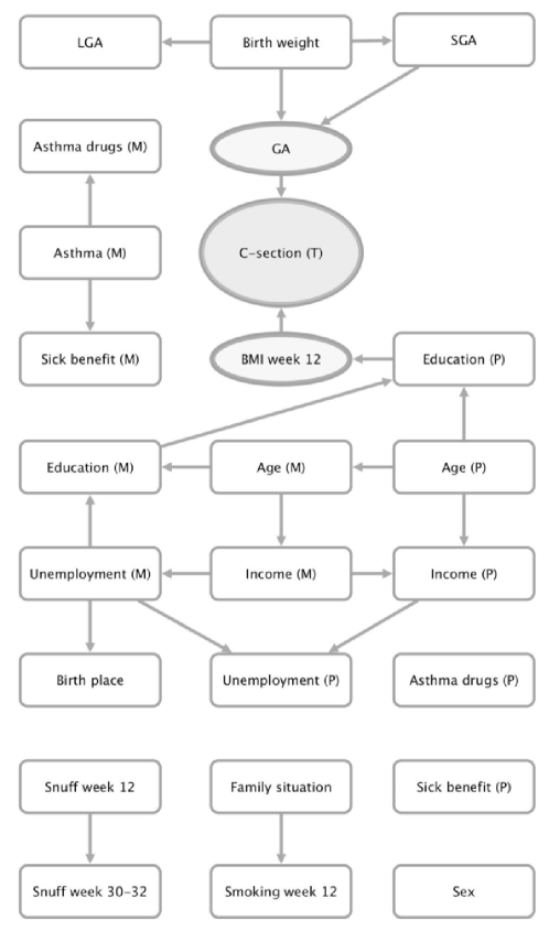
Figure 5: DAG resulting from MMHC, $\widehat{X}_{\rightarrow T}$.

The results from the covariate selection algorithms are summarized in Tables 1-24 in Appendix B, where selection success rates and median cardinality of the selected sets are presented. Three definitions of success are used for the selected subset, $\widehat{S}$; i) unconfoundedness holds, i.e., $\big{(}Y(1),Y(0)\big{)}\perp\!\!\!\perp T\mid\widehat{S}$, ii) the target subset is included in the selected subset ($S\subseteq\widehat{S}$), and iii) equal subsets ($S=\widehat{S}$). The tables also include empirical bias, standard deviation and MSE for the ACE estimation as well as confidence interval coverage, mean width and mean lower and upper confidence interval limits. Results for Setting 1, $n=2000$, are illustrated in Figures 3-5. Results for $\widehat{W}_{\rightarrow Y}$ are omitted throughout due to the fact that when the causal structure is estimated $\widehat{W}_{\rightarrow Y}$ and $\widehat{X}_{\rightarrow Y}$ turn out to be virtually identical.

In Setting 1, when the sample size is relatively small ($n=500$, $n=1000$) neither of the network algorithms succeed in selecting only sets that uphold unconfoundedness. MMPC has in these cases higher rates of success than MMHC. For the linear outcome model, when $n=500$ the success rates for MMPC and MMHC are in the range [63.6, 99.2] and [31.6, 88.2], respectively, and for $n=1000$ the ranges are [94.9, 100.0] and [66.1, 98.8]. However, when the sample size is relatively large ($n=2000$, $n=10000$) virtually all selected sets have 100% success rate in upholding unconfoundedness (the exception is the $\widehat{Q}_{\rightarrow T}$ sets with success rates 99.8 when $n=2000$), and this is the case for both network algorithms. For the larger sample sizes MMPC and MMHC not only select sets that uphold unconfoundedness, they frequently manage to exactly select the target subsets. For the binary outcome model, when $n=500$ the success rates for MMPC and MMHC are in the range [57.3, 97.7] and [29.0, 85.4], respectively, and for $n=1000$ the ranges are [92.8, 100.0] and [70.7, 99.2]. For the larger sample sizes the results are similar to the linear outcome case. For the nonlinear outcome model, when $n=500$ the success rates for MMPC and MMHC are in the range [83.2, 99.9] and [43.6, 99.7], respectively, and for $n=1000$ the success rates are 100.0 for all sets selected by MMPC and in the range [96.9, 100.0] for MMHC. For the larger sample sizes all sets have 100% success rate and both methods frequently manage to exactly select the target subsets.

RF performs similar to MMPC and MMHC with the important exception that it is, regardless of outcome model, unable to select the minimal target subsets $Q_{\rightarrow T}$ and $Z_{\rightarrow Y}$ with any desirable accuracy. Also, for the nonlinear outcome model case, RF fails when estimating the set $X_{\rightarrow Y}$.

Due to the fact that implementing the LASSO in a high-dimensional covariate space was much more time consuming than the other three methods, the investigation of LASSO is limited to $n=500,1000,2000$. LASSO is the only method that is able, regardless of sample size, to select sets that virtually always uphold unconfoundedness. However, sets selected by LASSO have much higher cardinality than the sets selected by the other three methods. Thus the dimension reduction is not as pronounced as with the other methods and the exact target sets are rarely selected. When $n=500,1000$, LASSO performs better than the other methods, while for the larger sample sizes sets selected by any of the network methods often result in smaller MSE than sets selected by LASSO.

The simulation settings for the linear and binary outcome cases in this paper are similar to the linear and binary outcome cases in Persson et al. (2017) which allow us to make some comparisons of the methods used here and the kernel smoothing method used in the latter paper. Note that the kernel smoothing procedure is very computer intensive and is not feasible for the relatively high dimensions studied in this paper. For $n=1000$ (the largest sample size studied in Persson et al. (2017)) and only 10 covariates in $X$ kernel smoothing performs marginally better than MMPC does (when $n=1000$ and 100 covariates), in terms of success rates in upholding unconfoundedness, but MMPC manages to exactly retrieve the target subsets much more frequently. MMHC on the other hand is outperformed by kernel smoothing for such a relatively small sample size.

When PSM is used, conditioning on one of the sets $X$, $\widehat{X}_{\rightarrow T}$ or $\widehat{X}_{\rightarrow T,Y}$ results in a considerable larger bias and variance than conditioning on any of the other sets (where success rates of upholding unconfoundedness are 100%). These results corroborates the results for PSM in Persson et al. (2017) in so far that, with very few exceptions, conditioning on $\widehat{Q}_{\rightarrow T}$ results in lower MSE than conditioning on $\widehat{X}_{\rightarrow T}$ but that conditioning on $\widehat{X}_{\rightarrow Y}$ or $\widehat{Z}_{\rightarrow Y}$ in turn results in lower MSE than conditioning on $\widehat{Q}_{\rightarrow T}$. However, as pointed out by an anonymous referee, these results are probably, at least partly, driven by the fact that PSM with main effects logistic regression is a poor estimation strategy, and not by the selected sets per se. Consequently, when TMLE together with BART is used, first of all we see that MSEs generally are much lower than when using PSM with logistic regression. Secondly, we see that in many cases reducing the covariate set prior to estimating ACE results in higher MSE compared to using $X$. Still, for large sample sizes, conditioning on $\widehat{X}_{\rightarrow Y}$ results in a reduction in MSE compared to conditioning on $X$ and conditioning on $\widehat{X}_{\rightarrow T,Y}$ results in reduced or equal MSE compared to $X$.

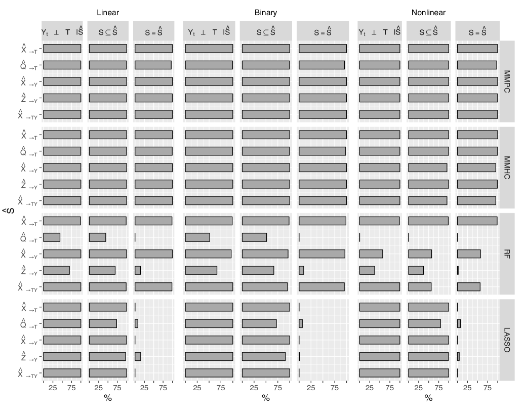
Figure 3: Simulation results for Setting 1, $n=2000$. Selection success rates (%) for the covariate sets ($\hat{S}$) selected by MMPC, MMHC, RF or LASSO. Definitions of success are; i) unconfoundedness holds ($Y_{t}\perp T|\hat{S}$), ii) the target subset is included in the selected subset ($S\subseteq\hat{S}$) and iii) equal subsets ($S=\hat{S}$). The selected covariates sets are: covariates predicting treatment $\widehat{X}_{\rightarrow T}$, covariates predicting outcome $\widehat{X}_{\rightarrow Y}$, covariates predicting both treatment and outcome $\widehat{Q}_{\rightarrow T}\subseteq\widehat{X}_{\rightarrow T}$, $\widehat{Z}_{\rightarrow Y}\subseteq\widehat{X}_{\rightarrow Y}$ and $\widehat{X}_{\rightarrow T,Y}=\widehat{X}_{\rightarrow T}\cup\widehat{X}_{\rightarrow Y}$.

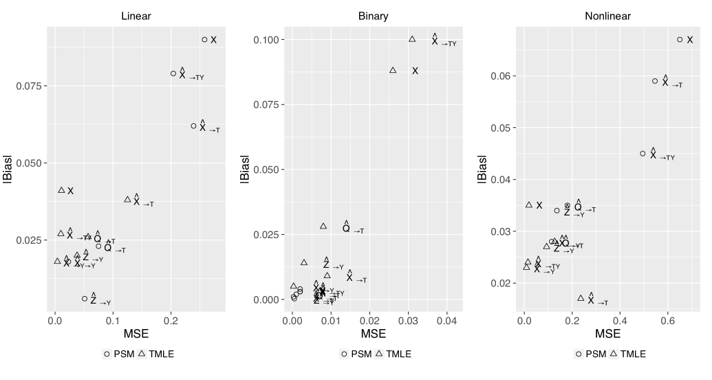
Figure 4: Simulation results for Setting 1, $n=2000$. Absolute bias and MSE are for the ACE estimated using different sets of covariates as selected by MMPC and either propensity score matching (PSM) or targeted maximum likelihood estimation (TMLE). The different covariates sets are: $X$, covariates predicting treatment $\widehat{X}_{\rightarrow T}$, covariates predicting outcome $\widehat{X}_{\rightarrow Y}$, covariates predicting both treatment and outcome $\widehat{Q}_{\rightarrow T}\subseteq\widehat{X}_{\rightarrow T}$, $\widehat{Z}_{\rightarrow Y}\subseteq\widehat{X}_{\rightarrow Y}$ and $\widehat{X}_{\rightarrow T,Y}=\widehat{X}_{\rightarrow T}\cup\widehat{X}_{\rightarrow Y}$.

In Setting 2, when unconfoundedness does not hold given $X$ the success rates are, as expected, very low. In Setting 2 there are two ways in which a set can fail to uphold unconfoundedness: 1) if it does not include $X_{4}$ and/or 2) if it includes $X_{9}$. For the larger sample sizes all methods select sets that include both $X_{4}$ and $X_{9}$ or include too few covariates, thus failing the unconfoundedness assumption. However, for PSM, except for $\widehat{X}_{\rightarrow T,Y}$, the sets selected by MMPC or MMHC often result in smaller bias and MSE compared to bias and MSE when conditioning on $X$. For TMLE it is only $\widehat{Q}_{\rightarrow T}$, $\widehat{X}_{\rightarrow Y}$ and $\widehat{Z}_{\rightarrow Y}$ that results in reduced MSE compared to $X$ for $n=10000$. Thus, in a situation where we are not perfectly sure that unconfoundedness is upheld when conditioning on $X$, at least for PSM, it does not seem to be harmful to use this confounder selection procedure for reducing the covariate set.

As mentioned in Section 5.3 implementing LASSO was more computer intensive than any of the methods MMPC, MMHC or RF. In Table 1 the computational times (measured by system.time) for $n=10000$ when only running the step where $\widehat{X}_{\rightarrow T}$ is estimated from $X$, i.e., mmpc, mmhc, cv.glmnet and randomForest are each run only once. Timings differ slightly between runs but the example in Table 1 give an accurate description of the difference between methods. The computations were run on a MacBook Pro (Early 2015) with 3,1 GHz Intel Core i7 Processor and 16 GB 1867 MHz DDR3 Memory.

Table 1: Computation time in seconds (and relative to MMPC) for $n=10000$ when only running the step were $X_{T}$ is estimated from $\{X,T\}$, i.e., mmpc, mmhc, cv.glmnet and randomForest are each run only once.

Method	Seconds	Rel
MMPC	1.1	1.0
MMHC	2.2	2.0
RF	78.2	71.1
LASSO	2114.3	1922.1

6 Data Analysis

Previous studies have indicated that children delivered by C-section are at an increased risk of developing wheezing and asthma (see, e.g., Magnus et al., 2011; Bråbäck et al., 2013). Here, we select covariates for estimating the ACE of being delivered by C-section on, before the age of four, being prescribed medication commonly used to treat asthma. Using record linkage register data from the Umeå SIMSAM Lab (Lindgren, Nilsson, de Luna, and Ivarsson, 2016) all children being the result of first-time mothers giving birth to full term (37 or more full weeks of gestation) singleton live offspring in the year 2006 in Sweden were identified ($n=41857$). From this population the subset of children being delivered by C-section or non-instrumental vaginal delivery, who were residents in Sweden during the whole study period, were offspring of two native Swedish parents and had no major malformations reported at birth were selected ($n=23817$). Using data from the Swedish Prescribed Drug Registry all children being prescribed drugs with one of the ATC-codes (WHO Collaborating Centre for Drug Statistics Methodology, 2014) R03AC, R03AK, R03BA, R03BC, R03CC, R03DC (hereinafter ”asthma drugs”) at least once before the age of four were identified.

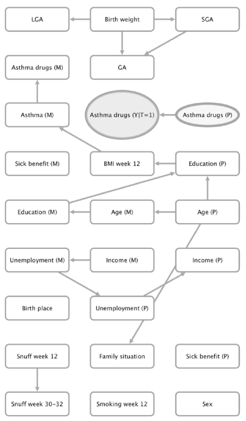
Figure 6: DAG resulting from MMHC, $\widehat{X}_{\rightarrow Y}^{1}$

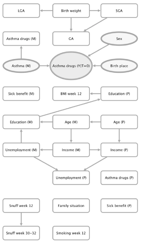
Figure 7: DAG resulting from MMHC, $\widehat{X}_{\rightarrow Y}^{0}$

As potential confounders we included 24 variables, listed in Table 25 in Appendix C. All observations with missing data on any of the covariates were excluded ($n=2950$), resulting in a complete cases sample containing $n=20867$ children. The proportion of children delivered by C-section was 20.9% and 39.7% of the children had been prescribed asthma drugs at least once before the age of four. MMPC and MMHC resulted in equal sets, namely: $\widehat{X}_{\rightarrow T}=${Maternal BMI at first antenatal visit, Gestational age}, $\widehat{Q}_{\rightarrow T}=${Maternal BMI at first antenatal visit}, $\widehat{X}_{\rightarrow Y}=${Maternal asthma, Paternal asthma drugs prescription within 6 months before delivery, Offspring sex, Birth place}, $\widehat{Z}_{\rightarrow Y}=${Offspring sex, Birth place}, $\widehat{X}_{\rightarrow T,Y}=\widehat{X}_{\rightarrow T}\cup\widehat{X}_{\rightarrow Y}$. The DAGs estimated by MMHC are given in Figures 1-7 in Appendix C (Cytoscape was used to visualize the graphs (Shannon et al., 2003)). PSM and TMLE were implemented as described in Section 5.2 and estimates of the ACE, i.e., risk difference, are presented in Table 2. For PSM the distributions of the estimated propensity scores for the different treatment groups were similar and exact matches were found when controlling for all sets except $X$ (where a caliper of 0.1 standard deviations of the estimated propensity score was used). The estimate based on raw data, not controlling for any confounders, suggest on average an 3.5% risk increase in being prescribed asthma drugs before the age of four if you are delivered by C-section compared to what would be the risk in case of non-instrumental vaginal delivery. For both PSM and TMLE, controlling for any of the selected covariate sets results in slightly lower point estimates, although all still statistically significant. Assuming that we have unconfoundedness given the 24 potential confounders we started with, and taking into consideration the results from the simulation study where controlling for $\widehat{X}_{\rightarrow Y}$ often was the best choice, the results in Table 2 suggest that the ACE lies in the range [0.012, 0.047].

Table 2: Estimates of the ACE. The cardinalities of the covariate sets (#), ACE estimates ($\hat{\beta}$), standard errors (SE; Abadie-Imbens for PSM and influence-curved based for TMLE), lower (CIL) and upper (CIU) limits of 95% confidence intervals.

$\hat{S}$	#	$\hat{\beta}$	SE	CIL	CIU
$\emptyset$	0	0.035	0.008	0.019	0.052
PSM
$X$	24	0.023	0.010	0.004	0.042
$\widehat{X}_{\rightarrow T}$	2	0.026	0.009	0.009	0.043
$\widehat{Q}_{\rightarrow T}$	1	0.031	0.008	0.015	0.048
$\widehat{X}_{\rightarrow Y}$	4	0.029	0.008	0.013	0.045
$\widehat{Z}_{\rightarrow Y}$	2	0.031	0.008	0.015	0.048
$\widehat{X}_{\rightarrow T,Y}$	6	0.021	0.009	0.004	0.038
TMLE
$X$	24	0.024	0.011	0.003	0.044
$\widehat{X}_{\rightarrow T}$	2	0.027	0.009	0.009	0.045
$\widehat{Q}_{\rightarrow T}$	1	0.032	0.009	0.014	0.049
$\widehat{X}_{\rightarrow Y}$	4	0.029	0.009	0.012	0.047
$\widehat{Z}_{\rightarrow Y}$	2	0.031	0.009	0.014	0.048
$\widehat{X}_{\rightarrow T,Y}$	6	0.025	0.010	0.006	0.044

7 Discussion

In this paper, we have introduced the network algorithms MMPC and MMHC in conjunction with the covariate selection algorithms in de Luna et al. (2011) as methods for confounder selection in causal inference when the true causal structure is not known. Given that unconfoundedness holds when conditioning on $X$, the approach was shown, for sufficiently large sample sizes, to accurately estimate certain target covariate subsets. Compared to RF and LASSO, the network algorithms were preferable both with regard to estimation of the ACE and with regard to computational efficiency. However, it is very likely that the performance of RF and LASSO could be improved upon by carefully selecting their respective tuning parameter (variable importance cut-off and regularization parameter). Also, as expected, none of the four methods investigated were able to select covariate sets that uphold unconfoundedness when the true causal structure included a collider of unmeasured causes of the outcome and treatment. This is due to the fact that the methods cannot distinguish association from causation and thus a collider will frequently be included in the selected covariate set. How much one in practice should worry about the $M$-bias scenario exemplified in Setting 5.1.2 is debatable. Rubin (2009), Liu et al. (2012) and Ding and Miratrix (2015) suggest that it is rather uncommon and might be more of mathematical than practical interest. Moreover, the simulation results show that even if $M$-bias is present reducing the the dimension of the covariate set might still be beneficial.

The real data analysis consisted of 20867 observations and 24 covariates and this relatively high dimensional data proved to be more than feasible for MMPC and MMHC.

Appendix A: Proof of Theorem 1 in Section 4.4

Proof. Let $G_{A,B}$ denote a graph involving only the variables in the sets $A$ and $B$. Consider the graphs $G_{X,T}$, $G_{X_{\rightarrow T},Y(t)}$, $G_{X,Y(t)}$, $G_{X_{\rightarrow Y},T}$ and $G_{X_{\rightarrow T,Y},Y(t)}$, $t=0,1$.

It follows from C3 that the above graphs are all DAGs since each of them is a subgraph of a DAG.

It follows from C4-C5 that there exist joint probability distributions $p_{X,T}$, $p_{X_{\rightarrow T},Y(t)}$, $p_{X,Y(t)}$, $p_{X_{\rightarrow Y},T}$ and $p_{X_{\rightarrow T,Y},Y(t)}$, $t=0,1$, such that the local Markov property holds and which are faithful to the respective subgraph.

Then, together with conditions C1-C2 and C6, it follows from Theorem 3 in Tsamardinos et al. (2006) that if in the estimated skeleton of $G_{X,T}$, produced by MMPC with input variables $\{X,T\}$, there is an edge connecting $T$ to $X_{j}\in X$ then $X_{j}$ is a parent of $T$. Hence, $\widehat{X}_{\rightarrow T}=X_{\rightarrow T}$. Similarly, if in the estimated skeleton of $G_{X_{\rightarrow T},Y(t)}$, $t=0,1$, produced by MMPC with input variables $\{X_{\rightarrow T},Y|T=t\}$, there is an edge connecting $Y|T=t$ to $X_{j}\in X_{\rightarrow T}$ then $X_{j}$ is a parent of $Y|T=t$, i.e., a parent of $Y(t)$ since $Y(t)\perp\!\!\!\perp T|X$. Hence, $\widehat{Q}_{\rightarrow T}^{t}=Q_{\rightarrow T}^{t}$, $t=0,1$ and therefore $\widehat{Q}_{\rightarrow T}=Q_{\rightarrow T}$. Analogously, $\widehat{X}_{\rightarrow Y}=X_{\rightarrow Y}$ and $\widehat{Z}_{\rightarrow}=Z_{\rightarrow Y}$. Since $\widehat{X}_{\rightarrow T,Y}=\widehat{X}_{\rightarrow T}\cup\widehat{X}_{\rightarrow Y}$ it follows that if $\widehat{X}_{\rightarrow T}=X_{\rightarrow T}$ and $\widehat{X}_{\rightarrow Y}=X_{\rightarrow Y}$ then $\widehat{X}_{\rightarrow T,Y}=X_{\rightarrow T,Y}$. Finally, according to the same reasoning as above using MMPC with input variables $(X_{\rightarrow T,Y},Y|T=t)$ results in $\widehat{W}_{\rightarrow Y}=W_{\rightarrow Y}$

Appendix B: Simulation results from Section 5.3

Table 3: Setting 1, linear outcome model, $n=500,1000$. The proportion (%) of times the selected subset, $\widehat{S}$, satisfies three conditions of unconfoundedness and the median cardinality of $\widehat{S}$ (#). Average bias (Bias), standard deviation (SD) and mean square error (MSE) from estimating ACE with PSM and TMLE.

							PSM			TMLE
$n$	Method	$\widehat{S}$	$Y_{t}\perp\!\!\!\perp T\mid\widehat{S}$	$S\subseteq\widehat{S}$	$S=\widehat{S}$	#	Bias	SD	MSE	Bias	SD	MSE
500		$X$	100.0	100.0	100.0	100	0.340	1.370	1.992	0.133	0.163	0.044
	MMPC	$\widehat{X}_{\rightarrow T}$	88.1	83.7	83.7	5	0.251	0.937	0.941	0.208	0.755	0.612
		$\widehat{Q}_{\rightarrow T}$	63.6	63.6	61.8	3	0.406	0.757	0.737	0.404	0.703	0.658
		$\widehat{X}_{\rightarrow Y}$	88.5	27.3	27.3	4	0.195	0.501	0.289	0.189	0.392	0.189
		$\widehat{Z}_{\rightarrow Y}$	84.9	84.9	84.0	3	0.195	0.586	0.381	0.197	0.526	0.316
		$\widehat{X}_{\rightarrow T,Y}$	99.2	28.4	28.4	7	0.176	0.791	0.656	0.101	0.319	0.112
	MMHC	$\widehat{X}_{\rightarrow T}$	46.2	15.7	15.7	4	0.791	1.045	1.718	0.772	0.920	1.442
		$\widehat{Q}_{\rightarrow T}$	31.6	31.6	31.2	2	0.857	0.829	1.421	0.848	0.808	1.371
		$\widehat{X}_{\rightarrow Y}$	72.1	15.6	15.6	4	0.363	0.597	0.488	0.363	0.526	0.409
		$\widehat{Z}_{\rightarrow Y}$	69.3	69.3	68.6	3	0.360	0.670	0.579	0.363	0.626	0.524
		$\widehat{X}_{\rightarrow T,Y}$	88.2	12.5	12.5	7	0.291	0.842	0.794	0.240	0.521	0.329
	RF	$\widehat{X}_{\rightarrow T}$	63.6	44.7	32.8	5	0.459	0.941	1.096	0.450	0.791	0.829
		$\widehat{Q}_{\rightarrow T}$	18.7	17.9	0.1	3	0.926	0.752	1.423	0.921	0.659	1.282
		$\widehat{X}_{\rightarrow Y}$	88.5	88.5	83.0	5	0.202	0.497	0.288	0.182	0.385	0.181
		$\widehat{Z}_{\rightarrow Y}$	38.5	38.5	0.0	3	0.609	0.606	0.738	0.615	0.537	0.666
		$\widehat{X}_{\rightarrow T,Y}$	96.9	38.9	28.8	7	0.165	0.728	0.557	0.108	0.282	0.091
	LASSO	$\widehat{X}_{\rightarrow T}$	100.0	100.0	0.0	22	0.061	0.971	0.948	0.058	0.502	0.256
		$\widehat{Q}_{\rightarrow T}$	100.0	75.5	1.6	9	0.055	0.616	0.382	0.062	0.427	0.186
		$\widehat{X}_{\rightarrow Y}$	100.0	100.0	0.0	30	0.157	0.550	0.327	0.112	0.152	0.036
		$\widehat{Z}_{\rightarrow Y}$	99.8	94.5	1.7	8	0.094	0.597	0.365	0.077	0.393	0.160
		$\widehat{X}_{\rightarrow T,Y}$	100.0	100.0	0.0	45	0.198	1.013	1.066	0.121	0.175	0.045
1000		$X$	100.0	100.0	100.0	100	0.128	0.789	0.638	0.057	0.128	0.020
	MMPC	$\widehat{X}_{\rightarrow T}$	100.0	100.0	100.0	5	0.103	0.691	0.488	0.038	0.496	0.248
		$\widehat{Q}_{\rightarrow T}$	94.9	94.9	91.7	3	0.094	0.459	0.219	0.088	0.403	0.170
		$\widehat{X}_{\rightarrow Y}$	100.0	100.0	100.0	5	0.025	0.218	0.048	0.029	0.087	0.008
		$\widehat{Z}_{\rightarrow Y}$	100.0	100.0	99.7	3	0.020	0.317	0.101	0.031	0.277	0.078
		$\widehat{X}_{\rightarrow T,Y}$	100.0	100.0	100.0	8	0.112	0.595	0.366	0.037	0.135	0.020
	MMHC	$\widehat{X}_{\rightarrow T}$	96.9	96.8	96.8	5	0.134	0.713	0.527	0.075	0.539	0.296
		$\widehat{Q}_{\rightarrow T}$	91.8	91.8	90.9	3	0.118	0.473	0.238	0.112	0.427	0.195
		$\widehat{X}_{\rightarrow Y}$	66.1	56.4	56.4	5	0.394	0.551	0.459	0.392	0.522	0.427
		$\widehat{Z}_{\rightarrow Y}$	66.1	66.1	65.3	3	0.390	0.577	0.485	0.394	0.562	0.471
		$\widehat{X}_{\rightarrow T,Y}$	98.8	89.0	89.0	8	0.121	0.610	0.387	0.052	0.204	0.044
	RF	$\widehat{X}_{\rightarrow T}$	89.6	82.6	81.3	5	0.211	0.726	0.572	0.150	0.584	0.364
		$\widehat{Q}_{\rightarrow T}$	29.9	29.7	0.0	3	0.774	0.682	1.063	0.769	0.623	0.979
		$\widehat{X}_{\rightarrow Y}$	97.9	97.9	97.9	5	0.049	0.277	0.079	0.054	0.198	0.042
		$\widehat{Z}_{\rightarrow Y}$	55.6	55.6	0.0	4	0.421	0.503	0.430	0.429	0.467	0.403
		$\widehat{X}_{\rightarrow T,Y}$	100.0	81.1	80.1	8	0.104	0.566	0.331	0.038	0.135	0.020
	LASSO	$\widehat{X}_{\rightarrow T}$	100.0	100.0	0.0	20	0.045	0.690	0.478	0.042	0.415	0.174
		$\widehat{Q}_{\rightarrow T}$	100.0	77.2	3.4	7	0.010	0.406	0.165	0.047	0.299	0.092
		$\widehat{X}_{\rightarrow Y}$	100.0	100.0	0.0	24	0.052	0.333	0.113	0.050	0.096	0.012
		$\widehat{Z}_{\rightarrow Y}$	100.0	95.7	5.2	6	0.027	0.378	0.143	0.046	0.276	0.078
		$\widehat{X}_{\rightarrow T,Y}$	100.0	100.0	0.0	38	0.114	0.649	0.434	0.058	0.128	0.020

Table 4: Setting 1, linear outcome model, $n=2000,10000$. The proportion (%) of times the selected subset, $\widehat{S}$, satisfies three conditions of unconfoundedness and the median cardinality of $\widehat{S}$ (#). Average bias (Bias), standard deviation (SD) and mean square error (MSE) from estimating ACE with PSM and TMLE.

							PSM			TMLE
$n$	Method	$\widehat{S}$	$Y_{t}\perp\!\!\!\perp T\mid\widehat{S}$	$S\subseteq\widehat{S}$	$S=\widehat{S}$	#	Bias	SD	MSE	Bias	SD	MSE
2000		$X$	100.0	100.0	100.0	100	0.090	0.500	0.258	0.041	0.099	0.011
	MMPC	$\widehat{X}_{\rightarrow T}$	100.0	100.0	99.9	5	0.062	0.484	0.239	0.038	0.351	0.125
		$\widehat{Q}_{\rightarrow T}$	99.8	99.8	96.8	3	0.023	0.274	0.075	0.026	0.237	0.057
		$\widehat{X}_{\rightarrow Y}$	100.0	100.0	100.0	5	0.018	0.151	0.023	0.018	0.062	0.004
		$\widehat{Z}_{\rightarrow Y}$	100.0	100.0	99.8	3	0.006	0.227	0.051	0.020	0.193	0.038
		$\widehat{X}_{\rightarrow T,Y}$	100.0	100.0	99.9	8	0.079	0.444	0.204	0.027	0.097	0.010
	MMHC	$\widehat{X}_{\rightarrow T}$	100.0	100.0	100.0	5	0.062	0.484	0.239	0.037	0.351	0.124
		$\widehat{Q}_{\rightarrow T}$	99.8	99.8	99.5	3	0.023	0.271	0.074	0.024	0.237	0.057
		$\widehat{X}_{\rightarrow Y}$	100.0	100.0	100.0	5	0.018	0.151	0.023	0.018	0.062	0.004
		$\widehat{Z}_{\rightarrow Y}$	100.0	100.0	99.9	3	0.006	0.227	0.051	0.019	0.193	0.038
		$\widehat{X}_{\rightarrow T,Y}$	100.0	100.0	100.0	8	0.079	0.444	0.204	0.027	0.097	0.010
	RF	$\widehat{X}_{\rightarrow T}$	99.0	98.8	98.8	5	0.072	0.492	0.247	0.048	0.362	0.134
		$\widehat{Q}_{\rightarrow T}$	44.0	44.0	0.0	3	0.617	0.627	0.774	0.618	0.599	0.741
		$\widehat{X}_{\rightarrow Y}$	99.9	99.9	99.9	5	0.019	0.153	0.024	0.020	0.073	0.006
		$\widehat{Z}_{\rightarrow Y}$	69.3	69.3	14.7	4	0.288	0.456	0.291	0.300	0.440	0.283
		$\widehat{X}_{\rightarrow T,Y}$	100.0	98.7	98.7	8	0.077	0.444	0.203	0.029	0.097	0.010
	LASSO	$\widehat{X}_{\rightarrow T}$	100.0	100.0	0.1	18	0.016	0.484	0.235	0.017	0.309	0.096
		$\widehat{Q}_{\rightarrow T}$	100.0	73.2	7.4	6	-0.006	0.270	0.073	0.018	0.210	0.044
		$\widehat{X}_{\rightarrow Y}$	100.0	100.0	0.0	18	0.031	0.205	0.043	0.030	0.070	0.006
		$\widehat{Z}_{\rightarrow Y}$	100.0	97.2	15.1	5	0.006	0.256	0.065	0.025	0.196	0.039
		$\widehat{X}_{\rightarrow T,Y}$	100.0	100.0	0.0	31	0.067	0.455	0.211	0.034	0.097	0.011
10000		$X$	100.0	100.0	100.0	100	0.015	0.202	0.041	0.018	0.040	0.002
	MMPC	$\widehat{X}_{\rightarrow T}$	100.0	100.0	99.9	5	0.014	0.220	0.049	0.021	0.147	0.022
		$\widehat{Q}_{\rightarrow T}$	100.0	100.0	94.1	3	0.012	0.117	0.014	0.012	0.107	0.012
		$\widehat{X}_{\rightarrow Y}$	100.0	100.0	100.0	5	0.002	0.056	0.003	0.006	0.025	0.001
		$\widehat{Z}_{\rightarrow Y}$	100.0	100.0	99.8	3	0.004	0.096	0.009	0.010	0.090	0.008
		$\widehat{X}_{\rightarrow T,Y}$	100.0	100.0	99.9	8	0.014	0.206	0.043	0.012	0.040	0.002
	MMHC	$\widehat{X}_{\rightarrow T}$	100.0	100.0	100.0	5	0.015	0.220	0.049	0.021	0.147	0.022
		$\widehat{Q}_{\rightarrow T}$	100.0	100.0	99.5	3	0.009	0.112	0.013	0.011	0.106	0.011
		$\widehat{X}_{\rightarrow Y}$	100.0	100.0	100.0	5	0.002	0.056	0.003	0.006	0.025	0.001
		$\widehat{Z}_{\rightarrow Y}$	100.0	100.0	99.8	3	0.004	0.096	0.009	0.010	0.089	0.008
		$\widehat{X}_{\rightarrow T,Y}$	100.0	100.0	100.0	8	0.014	0.206	0.043	0.012	0.040	0.002
	RF	$\widehat{X}_{\rightarrow T}$	100.0	100.0	100.0	5	0.015	0.220	0.049	0.021	0.147	0.022
		$\widehat{Q}_{\rightarrow T}$	98.5	98.5	0.0	4	0.026	0.202	0.041	0.029	0.183	0.034
		$\widehat{X}_{\rightarrow Y}$	100.0	100.0	100.0	5	0.002	0.056	0.003	0.006	0.025	0.001
		$\widehat{Z}_{\rightarrow Y}$	80.1	80.1	80.1	3	0.191	0.386	0.185	0.201	0.396	0.197
		$\widehat{X}_{\rightarrow T,Y}$	100.0	100.0	100.0	8	0.014	0.206	0.043	0.011	0.040	0.002

Table 5: Setting 1, binary outcome model, $n=500,1000$. The proportion (%) of times the selected subset, $\widehat{S}$, satisfies three conditions of unconfoundedness and the median cardinality of $\widehat{S}$ (#). Average bias (Bias), standard deviation (SD) and mean square error (MSE) from estimating ACE with PSM and TMLE.

							PSM			TMLE
$n$	Method	$\widehat{S}$	$Y_{t}\perp\!\!\!\perp T\mid\widehat{S}$	$S\subseteq\widehat{S}$	$S=\widehat{S}$	#	Bias	SD	MSE	Bias	SD	MSE
500		$X$	100.0	100.0	100.0	100	-0.016	0.132	0.018	-0.066	0.079	0.011
	MMPC	$\widehat{X}_{\rightarrow T}$	88.1	83.7	83.7	5	-0.011	0.081	0.007	-0.037	0.147	0.023
		$\widehat{Q}_{\rightarrow T}$	57.3	57.3	55.6	3	-0.025	0.062	0.004	-0.074	0.121	0.020
		$\widehat{X}_{\rightarrow Y}$	68.4	28.5	28.2	4	-0.024	0.052	0.003	-0.034	0.061	0.005
		$\widehat{Z}_{\rightarrow Y}$	66.4	66.4	65.9	3	-0.021	0.056	0.004	-0.048	0.095	0.011
		$\widehat{X}_{\rightarrow T,Y}$	97.7	38.1	37.8	7	-0.009	0.077	0.006	-0.056	0.147	0.025
	MMHC	$\widehat{X}_{\rightarrow T}$	46.2	15.7	15.7	4	-0.046	0.084	0.009	-0.062	0.140	0.023
		$\widehat{Q}_{\rightarrow T}$	29.0	29.0	28.4	2	-0.050	0.065	0.007	-0.110	0.136	0.030
		$\widehat{X}_{\rightarrow Y}$	60.7	21.2	21.1	4	-0.028	0.053	0.004	-0.040	0.068	0.006
		$\widehat{Z}_{\rightarrow Y}$	59.1	59.1	58.6	3	-0.025	0.057	0.004	-0.053	0.098	0.012
		$\widehat{X}_{\rightarrow T,Y}$	85.4	17.8	17.8	7	-0.017	0.077	0.006	-0.056	0.145	0.024
	RF	$\widehat{X}_{\rightarrow T}$	63.2	44.6	33.1	5	-0.023	0.078	0.007	-0.053	0.137	0.022
		$\widehat{Q}_{\rightarrow T}$	24.6	24.2	0.0	3	-0.049	0.065	0.007	-0.080	0.090	0.015
		$\widehat{X}_{\rightarrow Y}$	35.0	35.0	17.0	5	-0.043	0.059	0.005	-0.053	0.052	0.006
		$\widehat{Z}_{\rightarrow Y}$	9.4	9.3	0.0	3	-0.059	0.054	0.006	-0.073	0.051	0.008
		$\widehat{X}_{\rightarrow T,Y}$	78.6	18.0	7.6	7	-0.014	0.073	0.005	-0.069	0.119	0.019
	LASSO	$\widehat{X}_{\rightarrow T}$	100.0	100.0	0.0	23	-0.003	0.089	0.008	-0.079	0.124	0.022
		$\widehat{Q}_{\rightarrow T}$	95.1	69.4	2.0	9	-0.004	0.063	0.004	-0.049	0.101	0.013
		$\widehat{X}_{\rightarrow Y}$	100.0	100.0	0.0	49	-0.010	0.073	0.005	-0.049	0.064	0.007
		$\widehat{Z}_{\rightarrow Y}$	99.8	92.7	0.7	12	-0.008	0.066	0.004	-0.046	0.104	0.013
		$\widehat{X}_{\rightarrow T,Y}$	100.0	100.0	0.0	60	-0.013	0.103	0.011	-0.064	0.084	0.011
1000		$X$	100.0	100.0	100.0	100	-0.006	0.071	0.005	-0.054	0.078	0.009
	MMPC	$\widehat{X}_{\rightarrow T}$	100.0	100.0	100.0	5	-0.006	0.060	0.004	-0.008	0.125	0.016
		$\widehat{Q}_{\rightarrow T}$	92.8	92.8	90.9	3	-0.006	0.039	0.002	-0.041	0.093	0.010
		$\widehat{X}_{\rightarrow Y}$	98.3	97.9	97.9	5	-0.002	0.029	0.001	-0.009	0.030	0.001
		$\widehat{Z}_{\rightarrow Y}$	98.3	98.3	98.0	3	-0.001	0.031	0.001	-0.023	0.069	0.005
		$\widehat{X}_{\rightarrow T,Y}$	100.0	99.6	99.6	8	-0.007	0.056	0.003	-0.081	0.146	0.028
	MMHC	$\widehat{X}_{\rightarrow T}$	96.9	96.8	96.8	5	-0.008	0.061	0.004	-0.011	0.124	0.016
		$\widehat{Q}_{\rightarrow T}$	89.9	89.9	88.5	3	-0.008	0.040	0.002	-0.042	0.093	0.010
		$\widehat{X}_{\rightarrow Y}$	70.7	59.1	59.1	5	-0.019	0.040	0.002	-0.026	0.036	0.002
		$\widehat{Z}_{\rightarrow Y}$	70.7	70.7	69.9	3	-0.019	0.042	0.002	-0.034	0.067	0.006
		$\widehat{X}_{\rightarrow T,Y}$	99.2	87.4	87.4	8	-0.007	0.057	0.003	-0.079	0.149	0.028
	RF	$\widehat{X}_{\rightarrow T}$	89.8	83.6	82.6	5	-0.013	0.061	0.004	-0.013	0.120	0.015
		$\widehat{Q}_{\rightarrow T}$	37.6	37.6	0.0	3	-0.040	0.053	0.004	-0.064	0.071	0.009
		$\widehat{X}_{\rightarrow Y}$	67.9	67.9	64.0	5	-0.020	0.040	0.002	-0.026	0.037	0.002
		$\widehat{Z}_{\rightarrow Y}$	35.1	35.1	0.0	3	-0.037	0.040	0.003	-0.046	0.038	0.004
		$\widehat{X}_{\rightarrow T,Y}$	97.8	55.6	52.9	8	-0.008	0.054	0.003	-0.080	0.148	0.028
	LASSO	$\widehat{X}_{\rightarrow T}$	100.0	100.0	0.0	20	-0.005	0.062	0.004	-0.043	0.121	0.016
		$\widehat{Q}_{\rightarrow T}$	99.7	74.0	2.6	8	-0.002	0.041	0.002	-0.029	0.096	0.010
		$\widehat{X}_{\rightarrow Y}$	100.0	100.0	0.0	54	-0.007	0.050	0.003	-0.039	0.066	0.006
		$\widehat{Z}_{\rightarrow Y}$	100.0	92.3	0.6	12	-0.004	0.047	0.002	-0.025	0.096	0.010
		$\widehat{X}_{\rightarrow T,Y}$	100.0	100.0	0.0	63	-0.008	0.065	0.004	-0.064	0.106	0.015

Table 6: Setting 1, binary outcome model, $n=2000,10000$. The proportion (%) of times the selected subset, $\widehat{S}$, satisfies three conditions of unconfoundedness and the median cardinality of $\widehat{S}$ (#). Average bias (Bias), standard deviation (SD) and mean square error (MSE) from estimating ACE with PSM and TMLE.

							PSM			TMLE
$n$	Method	$\widehat{S}$	$Y_{t}\perp\!\!\!\perp T\mid\widehat{S}$	$S\subseteq\widehat{S}$	$S=\widehat{S}$	#	Bias	SD	MSE	Bias	SD	MSE
2000		$X$	100.0	100.0	100.0	100	-0.003	0.046	0.002	-0.088	0.137	0.026
	MMPC	$\widehat{X}_{\rightarrow T}$	100.0	100.0	99.9	5	-0.003	0.043	0.002	-0.009	0.094	0.009
		$\widehat{Q}_{\rightarrow T}$	99.6	99.6	95.7	3	-0.002	0.026	0.001	-0.028	0.083	0.008
		$\widehat{X}_{\rightarrow Y}$	100.0	100.0	100.0	5	-0.001	0.019	3e-04	-0.005	0.016	3e-04
		$\widehat{Z}_{\rightarrow Y}$	100.0	100.0	99.8	3	2e-04	0.022	5e-04	-0.014	0.056	0.003
		$\widehat{X}_{\rightarrow T,Y}$	100.0	100.0	99.9	8	-0.004	0.041	0.002	-0.100	0.145	0.031
	MMHC	$\widehat{X}_{\rightarrow T}$	100.0	100.0	100.0	5	-0.003	0.043	0.002	-0.009	0.095	0.009
		$\widehat{Q}_{\rightarrow T}$	99.6	99.6	98.0	3	-0.002	0.026	0.001	-0.026	0.078	0.007
		$\widehat{X}_{\rightarrow Y}$	100.0	100.0	100.0	5	-0.001	0.019	3e-04	-0.005	0.016	3e-04
		$\widehat{Z}_{\rightarrow Y}$	100.0	100.0	99.9	3	2e-04	0.022	5e-04	-0.011	0.047	0.002
		$\widehat{X}_{\rightarrow T,Y}$	100.0	100.0	100.0	8	-0.004	0.041	0.002	-0.096	0.144	0.030
	RF	$\widehat{X}_{\rightarrow T}$	98.8	98.7	98.7	5	-0.004	0.044	0.002	-0.014	0.091	0.009
		$\widehat{Q}_{\rightarrow T}$	51.3	51.3	0.0	4	-0.031	0.046	0.003	-0.046	0.051	0.005
		$\widehat{X}_{\rightarrow Y}$	96.5	96.5	96.4	5	-0.003	0.022	5e-04	-0.008	0.020	4e-04
		$\widehat{Z}_{\rightarrow Y}$	66.6	66.6	9.7	4	-0.018	0.032	0.001	-0.026	0.038	0.002
		$\widehat{X}_{\rightarrow T,Y}$	100.0	95.2	95.2	8	-0.004	0.041	0.002	-0.097	0.148	0.031
	LASSO	$\widehat{X}_{\rightarrow T}$	100.0	100.0	0.0	18	-0.001	0.043	0.002	-0.033	0.117	0.015
		$\widehat{Q}_{\rightarrow T}$	100.0	72.0	6.8	7	-2e-05	0.028	0.001	-0.021	0.081	0.007
		$\widehat{X}_{\rightarrow Y}$	100.0	100.0	0.0	54	-0.003	0.034	0.001	-0.054	0.110	0.015
		$\widehat{Z}_{\rightarrow Y}$	100.0	90.9	1.3	10	-0.002	0.033	0.001	-0.021	0.108	0.012
		$\widehat{X}_{\rightarrow T,Y}$	100.0	100.0	0.0	62	-0.003	0.044	0.002	-0.092	0.134	0.026
10000		$X$	100.0	100.0	100.0	100	-4e-04	0.018	3e-04	-0.150	0.130	0.040
	MMPC	$\widehat{X}_{\rightarrow T}$	100.0	100.0	99.9	5	-0.001	0.018	3e-04	-0.012	0.055	0.003
		$\widehat{Q}_{\rightarrow T}$	100.0	100.0	97.3	3	-4e-04	0.010	1e-04	-0.016	0.067	0.005
		$\widehat{X}_{\rightarrow Y}$	100.0	100.0	100.0	5	2e-05	0.008	6e-05	-0.002	0.007	5e-05
		$\widehat{Z}_{\rightarrow Y}$	100.0	100.0	99.8	3	-9e-05	0.009	8e-05	-0.004	0.025	0.001
		$\widehat{X}_{\rightarrow T,Y}$	100.0	100.0	99.9	8	-0.001	0.017	3e-04	-0.146	0.127	0.038
	MMHC	$\widehat{X}_{\rightarrow T}$	100.0	100.0	100.0	5	-0.001	0.018	3e-04	-0.012	0.055	0.003
		$\widehat{Q}_{\rightarrow T}$	100.0	100.0	98.8	3	-4e-04	0.010	1e-04	-0.013	0.060	0.004
		$\widehat{X}_{\rightarrow Y}$	100.0	100.0	100.0	5	2e-05	0.008	6e-05	-0.002	0.007	5e-05
		$\widehat{Z}_{\rightarrow Y}$	100.0	100.0	99.8	3	-9e-05	0.009	8e-05	-0.003	0.022	0.001
		$\widehat{X}_{\rightarrow T,Y}$	100.0	100.0	100.0	8	-0.001	0.017	3e-04	-0.146	0.128	0.038
	RF	$\widehat{X}_{\rightarrow T}$	100.0	100.0	100.0	5	-0.001	0.018	3e-04	-0.013	0.055	0.003
		$\widehat{Q}_{\rightarrow T}$	82.7	82.7	36.3	3	-0.011	0.025	0.001	-0.022	0.046	0.003
		$\widehat{X}_{\rightarrow Y}$	100.0	100.0	100.0	5	2e-05	0.008	6e-05	-0.002	0.007	5e-05
		$\widehat{Z}_{\rightarrow Y}$	80.4	80.4	80.4	3	-0.011	0.024	0.001	-0.015	0.033	0.001
		$\widehat{X}_{\rightarrow T,Y}$	100.0	100.0	100.0	8	-0.001	0.017	3e-04	-0.148	0.129	0.038

Table 7: Setting 1, nonlinear outcome model, $n=500,1000$. The proportion (%) of times the selected subset, $\widehat{S}$, satisfies three conditions of unconfoundedness and the median cardinality of $\widehat{S}$ (#). Average bias (Bias), standard deviation (SD) and mean square error (MSE) from estimating ACE with PSM and TMLE.

							PSM			TMLE
$n$	Method	$\widehat{S}$	$Y_{t}\perp\!\!\!\perp T\mid\widehat{S}$	$S\subseteq\widehat{S}$	$S=\widehat{S}$	#	Bias	SD	MSE	Bias	SD	MSE
500		$X$	100.0	100.0	100.0	100	0.286	2.077	4.396	0.013	0.279	0.078
	MMPC	$\widehat{X}_{\rightarrow T}$	88.1	83.7	83.7	5	0.275	1.310	1.791	0.086	0.998	1.003
		$\widehat{Q}_{\rightarrow T}$	83.2	83.2	81.8	3	0.172	0.906	0.850	0.145	0.791	0.647
		$\widehat{X}_{\rightarrow Y}$	99.0	12.2	12.1	4	-0.033	0.712	0.508	-0.019	0.388	0.151
		$\widehat{Z}_{\rightarrow Y}$	95.2	95.2	94.4	3	0.022	0.756	0.572	0.010	0.639	0.408
		$\widehat{X}_{\rightarrow T,Y}$	99.9	11.2	11.1	7	0.154	1.198	1.459	-0.051	0.513	0.266
	MMHC	$\widehat{X}_{\rightarrow T}$	46.2	15.7	15.7	4	0.883	1.280	2.417	0.768	1.119	1.843
		$\widehat{Q}_{\rightarrow T}$	43.6	43.6	42.9	2	0.664	0.953	1.350	0.650	0.896	1.226
		$\widehat{X}_{\rightarrow Y}$	98.4	7.2	7.2	4	-0.025	0.723	0.523	-0.011	0.420	0.176
		$\widehat{Z}_{\rightarrow Y}$	95.0	95.0	93.9	3	0.026	0.768	0.591	0.013	0.652	0.425
		$\widehat{X}_{\rightarrow T,Y}$	99.7	4.3	4.3	7	0.167	1.153	1.357	-0.038	0.518	0.269
	RF	$\widehat{X}_{\rightarrow T}$	63.6	44.7	32.8	5	0.457	1.257	1.787	0.342	1.021	1.158
		$\widehat{Q}_{\rightarrow T}$	6.1	5.7	0.1	3	1.028	0.907	1.879	0.988	0.747	1.533
		$\widehat{X}_{\rightarrow Y}$	52.5	52.2	17.3	5	0.498	0.787	0.867	0.455	0.533	0.491
		$\widehat{Z}_{\rightarrow Y}$	13.9	13.7	0.0	4	0.853	0.792	1.354	0.876	0.623	1.156
		$\widehat{X}_{\rightarrow T,Y}$	84.6	21.9	5.9	8	0.255	1.152	1.393	0.125	0.481	0.247
	LASSO	$\widehat{X}_{\rightarrow T}$	100.0	100.0	0.0	22	0.166	1.414	2.027	-0.082	0.714	0.517
		$\widehat{Q}_{\rightarrow T}$	99.5	75.6	4.9	7	0.139	0.944	0.910	0.022	0.643	0.414
		$\widehat{X}_{\rightarrow Y}$	100.0	100.0	0.0	31	0.270	1.045	1.166	0.010	0.241	0.058
		$\widehat{Z}_{\rightarrow Y}$	99.8	94.6	1.5	9	0.256	0.978	1.023	0.040	0.606	0.369
		$\widehat{X}_{\rightarrow T,Y}$	100.0	100.0	0.0	46	0.266	1.521	2.383	-0.002	0.272	0.074
1000		$X$	100.0	100.0	100.0	100	0.161	1.192	1.448	-0.034	0.196	0.039
	MMPC	$\widehat{X}_{\rightarrow T}$	100.0	100.0	100.0	5	0.072	0.959	0.926	-0.029	0.685	0.471
		$\widehat{Q}_{\rightarrow T}$	100.0	100.0	98.5	3	-0.034	0.606	0.369	-0.042	0.510	0.262
		$\widehat{X}_{\rightarrow Y}$	100.0	64.6	64.6	5	-0.043	0.490	0.242	-0.029	0.195	0.039
		$\widehat{Z}_{\rightarrow Y}$	100.0	100.0	99.5	3	-0.039	0.533	0.285	-0.031	0.449	0.202
		$\widehat{X}_{\rightarrow T,Y}$	100.0	64.6	64.6	8	0.080	0.944	0.897	-0.036	0.272	0.075
	MMHC	$\widehat{X}_{\rightarrow T}$	96.9	96.8	96.8	5	0.111	0.969	0.952	0.007	0.716	0.513
		$\widehat{Q}_{\rightarrow T}$	96.9	96.9	96.6	3	-0.003	0.629	0.396	-0.012	0.539	0.290
		$\widehat{X}_{\rightarrow Y}$	99.7	32.3	32.3	4	-0.042	0.499	0.251	-0.023	0.241	0.059
		$\widehat{Z}_{\rightarrow Y}$	99.7	99.7	99.3	3	-0.036	0.535	0.288	-0.026	0.451	0.204
		$\widehat{X}_{\rightarrow T,Y}$	100.0	32.5	32.5	7	0.087	0.943	0.897	-0.037	0.331	0.111
	RF	$\widehat{X}_{\rightarrow T}$	89.6	82.6	81.3	5	0.174	0.998	1.026	0.082	0.745	0.562
		$\widehat{Q}_{\rightarrow T}$	2.6	2.5	0.0	3	1.041	0.636	1.489	1.016	0.544	1.329
		$\widehat{X}_{\rightarrow Y}$	57.6	57.6	55.7	5	0.392	0.632	0.553	0.389	0.504	0.406
		$\widehat{Z}_{\rightarrow Y}$	29.9	29.9	0.0	3	0.639	0.621	0.794	0.650	0.531	0.705
		$\widehat{X}_{\rightarrow T,Y}$	96.2	45.8	44.1	7	0.095	0.921	0.858	0.004	0.298	0.089
	LASSO	$\widehat{X}_{\rightarrow T}$	100.0	100.0	0.0	20	0.072	1.036	1.079	-0.074	0.579	0.341
		$\widehat{Q}_{\rightarrow T}$	100.0	79.3	4.7	7	0.081	0.667	0.451	-0.031	0.460	0.212
		$\widehat{X}_{\rightarrow Y}$	100.0	100.0	0.0	24	0.121	0.688	0.488	-0.023	0.165	0.028
		$\widehat{Z}_{\rightarrow Y}$	100.0	97.1	4.0	7	0.140	0.671	0.470	-0.014	0.469	0.220
		$\widehat{X}_{\rightarrow T,Y}$	100.0	100.0	0.0	38	0.124	1.035	1.086	-0.032	0.191	0.038

Table 8: Setting 1, nonlinear outcome model, $n=2000,10000$. The proportion (%) of times the selected subset, $\widehat{S}$, satisfies three conditions of unconfoundedness and the median cardinality of $\widehat{S}$ (#). Average bias (Bias), standard deviation (SD) and mean square error (MSE) from estimating ACE with PSM and TMLE.

							PSM			TMLE
$n$	Method	$\widehat{S}$	$Y_{t}\perp\!\!\!\perp T\mid\widehat{S}$	$S\subseteq\widehat{S}$	$S=\widehat{S}$	#	Bias	SD	MSE	Bias	SD	MSE
2000		$X$	100.0	100.0	100.0	100	0.067	0.803	0.650	-0.035	0.134	0.019
	MMPC	$\widehat{X}_{\rightarrow T}$	100.0	100.0	99.9	5	0.059	0.737	0.546	-0.017	0.485	0.236
		$\widehat{Q}_{\rightarrow T}$	100.0	100.0	97.7	3	-0.035	0.423	0.180	-0.028	0.355	0.127
		$\widehat{X}_{\rightarrow Y}$	100.0	100.0	100.0	5	-0.028	0.336	0.114	-0.023	0.090	0.009
		$\widehat{Z}_{\rightarrow Y}$	100.0	100.0	99.8	3	-0.034	0.368	0.136	-0.027	0.304	0.093
		$\widehat{X}_{\rightarrow T,Y}$	100.0	100.0	99.9	8	0.045	0.702	0.495	-0.024	0.119	0.015
	MMHC	$\widehat{X}_{\rightarrow T}$	100.0	100.0	100.0	5	0.059	0.736	0.546	-0.016	0.482	0.232
		$\widehat{Q}_{\rightarrow T}$	100.0	100.0	99.9	3	-0.038	0.417	0.176	-0.031	0.351	0.124
		$\widehat{X}_{\rightarrow Y}$	100.0	95.5	95.5	5	-0.028	0.336	0.114	-0.020	0.095	0.009
		$\widehat{Z}_{\rightarrow Y}$	100.0	100.0	99.3	3	-0.033	0.366	0.135	-0.025	0.302	0.092
		$\widehat{X}_{\rightarrow T,Y}$	100.0	95.5	95.5	8	0.043	0.704	0.497	-0.020	0.134	0.018
	RF	$\widehat{X}_{\rightarrow T}$	99.0	98.8	98.8	5	0.066	0.742	0.554	-0.007	0.498	0.248
		$\widehat{Q}_{\rightarrow T}$	0.2	0.2	0.0	3	1.079	0.441	1.358	1.068	0.348	1.262
		$\widehat{X}_{\rightarrow Y}$	57.3	57.3	57.3	5	0.392	0.548	0.454	0.402	0.492	0.404
		$\widehat{Z}_{\rightarrow Y}$	37.3	37.3	2.0	3	0.573	0.539	0.618	0.579	0.490	0.575
		$\widehat{X}_{\rightarrow T,Y}$	99.8	56.4	56.4	8	0.048	0.712	0.509	-0.013	0.159	0.025
	LASSO	$\widehat{X}_{\rightarrow T}$	100.0	100.0	0.1	18	0.041	0.753	0.568	-0.036	0.431	0.187
		$\widehat{Q}_{\rightarrow T}$	100.0	79.6	7.5	6	0.026	0.464	0.216	-0.001	0.330	0.109
		$\widehat{X}_{\rightarrow Y}$	100.0	100.0	0.0	18	0.057	0.461	0.216	-0.020	0.107	0.012
		$\widehat{Z}_{\rightarrow Y}$	100.0	99.2	4.5	6	0.083	0.461	0.220	0.011	0.337	0.114
		$\widehat{X}_{\rightarrow T,Y}$	100.0	100.0	0.0	31	0.037	0.748	0.561	-0.021	0.126	0.016
10000		$X$	100.0	100.0	100.0	100	0.003	0.344	0.118	-0.019	0.058	0.004
	MMPC	$\widehat{X}_{\rightarrow T}$	100.0	100.0	99.9	5	0.001	0.349	0.122	-0.013	0.220	0.049
		$\widehat{Q}_{\rightarrow T}$	100.0	100.0	98.1	3	-0.009	0.179	0.032	-0.004	0.149	0.022
		$\widehat{X}_{\rightarrow Y}$	100.0	100.0	100.0	5	-0.011	0.135	0.018	-0.007	0.039	0.002
		$\widehat{Z}_{\rightarrow Y}$	100.0	100.0	99.8	3	-0.012	0.152	0.023	-0.001	0.130	0.017
		$\widehat{X}_{\rightarrow T,Y}$	100.0	100.0	99.9	8	0.005	0.337	0.114	-0.008	0.050	0.003
	MMHC	$\widehat{X}_{\rightarrow T}$	100.0	100.0	100.0	5	0.002	0.349	0.122	-0.010	0.221	0.049
		$\widehat{Q}_{\rightarrow T}$	100.0	100.0	99.8	3	-0.009	0.176	0.031	-0.004	0.148	0.022
		$\widehat{X}_{\rightarrow Y}$	100.0	100.0	100.0	5	-0.011	0.135	0.018	-0.006	0.039	0.002
		$\widehat{Z}_{\rightarrow Y}$	100.0	100.0	99.8	3	-0.012	0.152	0.023	-5e-04	0.131	0.017
		$\widehat{X}_{\rightarrow T,Y}$	100.0	100.0	100.0	8	0.004	0.337	0.114	-0.007	0.050	0.003
	RF	$\widehat{X}_{\rightarrow T}$	100.0	100.0	100.0	5	0.002	0.349	0.122	-0.010	0.220	0.048
		$\widehat{Q}_{\rightarrow T}$	0.0	0.0	0.0	3	1.085	0.188	1.213	1.080	0.156	1.192
		$\widehat{X}_{\rightarrow Y}$	54.5	54.5	54.5	5	0.443	0.485	0.431	0.441	0.490	0.435
		$\widehat{Z}_{\rightarrow Y}$	40.4	40.4	40.4	2	0.574	0.475	0.555	0.582	0.477	0.566
		$\widehat{X}_{\rightarrow T,Y}$	100.0	54.5	54.5	8	0.008	0.337	0.114	-0.006	0.066	0.004

Table 9: Setting 2, linear outcome model, $n=500,1000$. The proportion (%) of times the selected subset, $\widehat{S}$, satisfies three conditions of unconfoundedness and the median cardinality of $\widehat{S}$ (#). Average bias (Bias), standard deviation (SD) and mean square error (MSE) from estimating ACE with PSM and TMLE.

							PSM			TMLE
$n$	Method	$\widehat{S}$	$Y_{t}\perp\!\!\!\perp T\mid\widehat{S}$	$S\subseteq\widehat{S}$	$S=\widehat{S}$	#	Bias	SD	MSE	Bias	SD	MSE
500		$X$	0.0	100.0	0.0	100	-2.263	2.141	9.702	-1.819	0.580	3.643
	MMPC	$\widehat{X}_{\rightarrow T}$	64.6	63.5	63.5	5	0.374	1.604	2.714	0.334	1.388	2.037
		$\widehat{Q}_{\rightarrow T}$	0.2	0.2	0.2	2	2.180	1.324	6.503	2.180	1.297	6.436
		$\widehat{X}_{\rightarrow Y}$	0.0	0.0	0.0	3	1.520	1.307	4.016	1.534	1.258	3.934
		$\widehat{Z}_{\rightarrow Y}$	0.0	0.6	0.2	2	1.884	1.402	5.515	1.898	1.362	5.457
		$\widehat{X}_{\rightarrow T,Y}$	0.0	1.1	0.0	7	-2.032	1.415	6.131	-2.133	0.983	5.517
	MMHC	$\widehat{X}_{\rightarrow T}$	10.3	8.1	8.1	4	1.146	1.473	3.484	1.109	1.259	2.816
		$\widehat{Q}_{\rightarrow T}$	0.0	0.0	0.0	2	2.323	1.224	6.895	2.334	1.188	6.858
		$\widehat{X}_{\rightarrow Y}$	0.0	0.0	0.0	3	1.569	1.285	4.112	1.592	1.237	4.064
		$\widehat{Z}_{\rightarrow Y}$	0.0	0.3	0.1	1	1.936	1.382	5.660	1.955	1.343	5.623
		$\widehat{X}_{\rightarrow T,Y}$	0.0	0.1	0.0	6	-1.328	1.350	3.586	-1.377	0.961	2.819
	RF	$\widehat{X}_{\rightarrow T}$	17.7	39.6	6.7	5	-1.373	1.643	4.584	-1.350	1.436	3.885
		$\widehat{Q}_{\rightarrow T}$	0.7	0.7	0.6	3	0.471	1.069	1.364	0.555	0.909	1.135
		$\widehat{X}_{\rightarrow Y}$	0.0	0.1	0.0	3	1.189	1.187	2.823	1.276	1.062	2.757
		$\widehat{Z}_{\rightarrow Y}$	0.0	0.0	0.0	3	1.168	1.194	2.789	1.252	1.073	2.718
		$\widehat{X}_{\rightarrow T,Y}$	0.0	0.4	0.0	7	-1.949	1.316	5.532	-1.919	0.911	4.512
	LASSO	$\widehat{X}_{\rightarrow T}$	9.9	100.0	0.0	27	-2.344	1.646	8.203	-2.163	0.894	5.476
		$\widehat{Q}_{\rightarrow T}$	5.7	84.4	0.2	18	-2.294	1.509	7.539	-2.106	0.968	5.371
		$\widehat{X}_{\rightarrow Y}$	0.0	100.0	0.0	50	-2.263	1.489	7.338	-1.913	0.597	4.015
		$\widehat{Z}_{\rightarrow Y}$	5.8	89.5	0.0	21	-2.293	1.438	7.325	-2.120	0.775	5.096
		$\widehat{X}_{\rightarrow T,Y}$	0.0	100.0	0.0	62	-2.323	1.837	8.771	-1.964	0.599	4.215
1000		$X$	0.0	100.0	0.0	100	-2.537	1.236	7.963	-2.494	0.439	6.414
	MMPC	$\widehat{X}_{\rightarrow T}$	75.5	98.7	75.5	5	-0.662	1.575	2.918	-0.697	1.378	2.385
		$\widehat{Q}_{\rightarrow T}$	8.0	9.2	7.9	3	0.856	1.299	2.421	0.870	1.238	2.290
		$\widehat{X}_{\rightarrow Y}$	0.0	2.1	0.0	4	0.166	1.098	1.233	0.191	1.045	1.128
		$\widehat{Z}_{\rightarrow Y}$	0.1	16.4	2.0	3	0.293	1.163	1.439	0.309	1.104	1.314
		$\widehat{X}_{\rightarrow T,Y}$	0.0	14.8	0.0	8	-2.716	0.982	8.340	-2.748	0.521	7.823
	MMHC	$\widehat{X}_{\rightarrow T}$	80.7	80.7	80.7	5	0.242	1.186	1.466	0.210	0.975	0.994
		$\widehat{Q}_{\rightarrow T}$	4.9	4.9	4.8	2	1.526	1.043	3.417	1.543	0.991	3.361
		$\widehat{X}_{\rightarrow Y}$	0.0	0.5	0.0	4	0.441	0.997	1.190	0.458	0.946	1.104
		$\widehat{Z}_{\rightarrow Y}$	0.0	7.6	1.1	3	0.559	1.068	1.454	0.566	1.011	1.343
		$\widehat{X}_{\rightarrow T,Y}$	0.0	7.7	0.0	8	-2.504	1.079	7.435	-2.539	0.714	6.957
	RF	$\widehat{X}_{\rightarrow T}$	14.0	77.4	11.9	6	-2.094	1.456	6.506	-2.131	1.237	6.073
		$\widehat{Q}_{\rightarrow T}$	0.0	0.0	0.0	3	0.351	0.793	0.752	0.396	0.692	0.636
		$\widehat{X}_{\rightarrow Y}$	0.0	0.0	0.0	3	1.582	1.015	3.535	1.634	0.969	3.609
		$\widehat{Z}_{\rightarrow Y}$	0.0	0.0	0.0	3	1.574	1.028	3.534	1.623	0.973	3.581
		$\widehat{X}_{\rightarrow T,Y}$	0.0	0.1	0.0	7	-2.509	1.077	7.453	-2.528	0.696	6.876
	LASSO	$\widehat{X}_{\rightarrow T}$	0.5	100.0	0.0	25	-2.746	1.100	8.748	-2.680	0.574	7.511
		$\widehat{Q}_{\rightarrow T}$	0.5	92.2	0.1	17	-2.653	0.991	8.022	-2.592	0.572	7.046
		$\widehat{X}_{\rightarrow Y}$	0.0	100.0	0.0	43	-2.503	0.993	7.251	-2.435	0.448	6.131
		$\widehat{Z}_{\rightarrow Y}$	0.4	85.0	0.0	19	-2.580	0.916	7.494	-2.542	0.559	6.775
		$\widehat{X}_{\rightarrow T,Y}$	0.0	100.0	0.0	55	-2.614	1.132	8.112	-2.569	0.441	6.794

Table 10: Setting 2, linear outcome model, $n=2000,10000$. The proportion (%) of times the selected subset, $\widehat{S}$, satisfies three conditions of unconfoundedness and the median cardinality of $\widehat{S}$ (#). Average bias (Bias), standard deviation (SD) and mean square error (MSE) from estimating ACE with PSM and TMLE.

							PSM			TMLE
$n$	Method	$\widehat{S}$	$Y_{t}\perp\!\!\!\perp T\mid\widehat{S}$	$S\subseteq\widehat{S}$	$S=\widehat{S}$	#	Bias	SD	MSE	Bias	SD	MSE
2000		$X$	0.0	100.0	0.0	100	-2.706	0.850	8.044	-2.735	0.352	7.606
	MMPC	$\widehat{X}_{\rightarrow T}$	15.5	100.0	15.5	6	-2.349	1.133	6.802	-2.436	1.027	6.987
		$\widehat{Q}_{\rightarrow T}$	7.7	40.1	7.7	4	-1.304	1.108	2.929	-1.290	1.071	2.812
		$\widehat{X}_{\rightarrow Y}$	0.0	17.3	0.0	5	-0.975	0.645	1.367	-0.957	0.597	1.273
		$\widehat{Z}_{\rightarrow Y}$	0.1	83.9	0.3	4	-0.976	0.684	1.421	-0.956	0.634	1.315
		$\widehat{X}_{\rightarrow T,Y}$	0.0	22.0	0.0	8	-2.743	0.726	8.051	-2.828	0.369	8.133
	MMHC	$\widehat{X}_{\rightarrow T}$	99.7	99.7	99.7	5	0.032	0.821	0.675	0.043	0.652	0.427
		$\widehat{Q}_{\rightarrow T}$	28.9	28.9	28.9	3	0.835	0.871	1.455	0.840	0.802	1.349
		$\widehat{X}_{\rightarrow Y}$	0.0	1.8	0.0	4	-0.140	0.565	0.338	-0.135	0.528	0.297
		$\widehat{Z}_{\rightarrow Y}$	0.0	18.3	0.0	3	-0.150	0.594	0.375	-0.130	0.556	0.326
		$\widehat{X}_{\rightarrow T,Y}$	0.0	17.9	0.0	8	-2.741	0.732	8.051	-2.820	0.383	8.097
	RF	$\widehat{X}_{\rightarrow T}$	9.6	97.5	9.5	6	-2.481	1.061	7.280	-2.557	0.906	7.361
		$\widehat{Q}_{\rightarrow T}$	0.0	0.0	0.0	3	0.211	0.598	0.402	0.242	0.525	0.334
		$\widehat{X}_{\rightarrow Y}$	0.0	0.0	0.0	3	2.175	1.020	5.771	2.186	0.995	5.770
		$\widehat{Z}_{\rightarrow Y}$	0.0	0.0	0.0	2	2.173	1.027	5.776	2.181	0.999	5.753
		$\widehat{X}_{\rightarrow T,Y}$	0.0	0.0	0.0	7	-2.704	0.741	7.859	-2.792	0.421	7.974
	LASSO	$\widehat{X}_{\rightarrow T}$	0.0	100.0	0.0	23	-2.805	0.795	8.499	-2.788	0.443	7.969
		$\widehat{Q}_{\rightarrow T}$	0.0	95.2	0.0	15	-2.747	0.721	8.067	-2.711	0.444	7.544
		$\widehat{X}_{\rightarrow Y}$	0.0	100.0	0.0	38	-2.640	0.700	7.458	-2.653	0.367	7.173
		$\widehat{Z}_{\rightarrow Y}$	0.0	85.8	0.0	17	-2.675	0.710	7.662	-2.686	0.424	7.392
		$\widehat{X}_{\rightarrow T,Y}$	0.0	100.0	0.0	49	-2.705	0.784	7.929	-2.758	0.341	7.721
10000		$X$	0.0	100.0	0.0	100	-2.839	0.358	8.185	-2.867	0.160	8.248
	MMPC	$\widehat{X}_{\rightarrow T}$	0.0	100.0	0.0	6	-2.834	0.367	8.166	-2.899	0.212	8.448
		$\widehat{Q}_{\rightarrow T}$	0.0	100.0	0.0	5	-2.545	0.253	6.542	-2.540	0.167	6.479
		$\widehat{X}_{\rightarrow Y}$	0.0	98.0	0.0	7	-2.300	0.377	5.434	-2.286	0.345	5.344
		$\widehat{Z}_{\rightarrow Y}$	0.0	99.9	0.0	5	-2.305	0.381	5.460	-2.287	0.351	5.353
		$\widehat{X}_{\rightarrow T,Y}$	0.0	98.1	0.0	9	-2.832	0.351	8.145	-2.902	0.159	8.449
	MMHC	$\widehat{X}_{\rightarrow T}$	0.0	100.0	0.0	6	-2.834	0.367	8.166	-2.898	0.210	8.443
		$\widehat{Q}_{\rightarrow T}$	0.0	100.0	0.0	5	-2.545	0.253	6.542	-2.541	0.168	6.485
		$\widehat{X}_{\rightarrow Y}$	0.0	49.0	0.0	6	-1.323	0.784	2.364	-1.302	0.776	2.296
		$\widehat{Z}_{\rightarrow Y}$	0.0	79.0	0.0	4	-1.322	0.789	2.371	-1.304	0.780	2.310
		$\widehat{X}_{\rightarrow T,Y}$	0.0	69.3	0.0	9	-2.832	0.351	8.145	-2.902	0.165	8.447
	RF	$\widehat{X}_{\rightarrow T}$	0.3	100.0	0.3	6	-2.826	0.390	8.137	-2.890	0.247	8.415
		$\widehat{Q}_{\rightarrow T}$	0.0	0.0	0.0	2	0.871	0.394	0.914	0.878	0.377	0.914
		$\widehat{X}_{\rightarrow Y}$	0.0	0.0	0.0	2	2.976	0.129	8.876	2.983	0.119	8.914
		$\widehat{Z}_{\rightarrow Y}$	0.0	0.0	0.0	2	2.977	0.130	8.881	2.982	0.119	8.905
		$\widehat{X}_{\rightarrow T,Y}$	0.0	0.0	0.0	7	-2.820	0.356	8.080	-2.893	0.193	8.406

Table 11: Setting 2, binary outcome model, $n=500,1000$. The proportion (%) of times the selected subset, $\widehat{S}$, satisfies three conditions of unconfoundedness and the median cardinality of $\widehat{S}$ (#). Average bias (Bias), standard deviation (SD) and mean square error (MSE) from estimating ACE with PSM and TMLE.

							PSM			TMLE
$n$	Method	$\widehat{S}$	$Y_{t}\perp\!\!\!\perp T\mid\widehat{S}$	$S\subseteq\widehat{S}$	$S=\widehat{S}$	#	Bias	SD	MSE	Bias	SD	MSE
500		$X$	0.0	100.0	0.0	100	0.095	0.103	0.019	0.015	0.080	0.007
	MMPC	$\widehat{X}_{\rightarrow T}$	64.6	63.5	63.5	5	-0.014	0.080	0.007	-0.097	0.173	0.039
		$\widehat{Q}_{\rightarrow T}$	0.3	0.3	0.3	2	-0.086	0.071	0.012	-0.122	0.173	0.045
		$\widehat{X}_{\rightarrow Y}$	0.0	0.0	0.0	3	-0.059	0.068	0.008	-0.065	0.068	0.009
		$\widehat{Z}_{\rightarrow Y}$	0.0	1.0	0.7	2	-0.074	0.071	0.011	-0.081	0.133	0.024
		$\widehat{X}_{\rightarrow T,Y}$	0.0	0.3	0.0	7	0.083	0.067	0.011	0.022	0.113	0.013
	MMHC	$\widehat{X}_{\rightarrow T}$	10.3	8.1	8.1	4	-0.047	0.078	0.008	-0.106	0.145	0.032
		$\widehat{Q}_{\rightarrow T}$	0.0	0.0	0.0	2	-0.094	0.065	0.013	-0.130	0.194	0.055
		$\widehat{X}_{\rightarrow Y}$	0.0	0.0	0.0	3	-0.061	0.067	0.008	-0.066	0.068	0.009
		$\widehat{Z}_{\rightarrow Y}$	0.0	0.3	0.2	2	-0.076	0.070	0.011	-0.084	0.134	0.025
		$\widehat{X}_{\rightarrow T,Y}$	0.0	0.0	0.0	6	0.056	0.067	0.008	0.004	0.119	0.014
	RF	$\widehat{X}_{\rightarrow T}$	17.5	39.1	6.8	5	0.055	0.076	0.009	-0.017	0.149	0.023
		$\widehat{Q}_{\rightarrow T}$	2.9	2.9	2.4	3	-0.008	0.056	0.003	-0.051	0.091	0.011
		$\widehat{X}_{\rightarrow Y}$	0.0	0.0	0.0	3	-0.069	0.065	0.009	-0.077	0.066	0.010
		$\widehat{Z}_{\rightarrow Y}$	0.0	0.1	0.0	3	-0.069	0.065	0.009	-0.078	0.067	0.011
		$\widehat{X}_{\rightarrow T,Y}$	0.0	0.3	0.0	7	0.079	0.063	0.010	0.020	0.097	0.010
	LASSO	$\widehat{X}_{\rightarrow T}$	9.9	100.0	0.2	27	0.093	0.076	0.014	0.004	0.107	0.011
		$\widehat{Q}_{\rightarrow T}$	5.6	71.3	0.1	17	0.083	0.070	0.012	0.013	0.109	0.012
		$\widehat{X}_{\rightarrow Y}$	0.0	96.8	0.0	48	0.087	0.068	0.012	0.022	0.076	0.006
		$\widehat{Z}_{\rightarrow Y}$	6.1	87.7	0.0	17	0.084	0.064	0.011	0.014	0.100	0.010
		$\widehat{X}_{\rightarrow T,Y}$	0.0	98.9	0.0	61	0.096	0.085	0.017	0.020	0.084	0.007
1000		$X$	0.0	100.0	0.0	100	0.098	0.058	0.013	0.039	0.072	0.007
	MMPC	$\widehat{X}_{\rightarrow T}$	75.5	98.7	75.5	5	0.025	0.071	0.006	-0.038	0.160	0.027
		$\widehat{Q}_{\rightarrow T}$	8.4	8.9	8.2	3	-0.034	0.058	0.005	-0.090	0.143	0.028
		$\widehat{X}_{\rightarrow Y}$	0.0	3.9	0.0	4	-0.003	0.052	0.003	-0.014	0.048	0.003
		$\widehat{Z}_{\rightarrow Y}$	0.2	17.4	2.4	3	-0.008	0.054	0.003	-0.025	0.077	0.006
		$\widehat{X}_{\rightarrow T,Y}$	0.0	16.8	0.0	8	0.104	0.043	0.013	0.045	0.113	0.015
	MMHC	$\widehat{X}_{\rightarrow T}$	80.7	80.7	80.7	5	-0.010	0.059	0.004	-0.087	0.152	0.031
		$\widehat{Q}_{\rightarrow T}$	6.6	6.6	6.5	2	-0.058	0.051	0.006	-0.122	0.153	0.038
		$\widehat{X}_{\rightarrow Y}$	0.0	1.8	0.0	4	-0.010	0.049	0.003	-0.019	0.046	0.002
		$\widehat{Z}_{\rightarrow Y}$	0.1	10.6	1.5	3	-0.015	0.051	0.003	-0.033	0.082	0.008
		$\widehat{X}_{\rightarrow T,Y}$	0.0	12.2	0.0	8	0.097	0.047	0.012	0.041	0.114	0.015
	RF	$\widehat{X}_{\rightarrow T}$	14.5	77.0	12.2	6	0.081	0.061	0.010	0.034	0.135	0.019
		$\widehat{Q}_{\rightarrow T}$	2.8	2.8	2.7	3	-0.006	0.038	0.001	-0.038	0.076	0.007
		$\widehat{X}_{\rightarrow Y}$	0.0	0.0	0.0	3	-0.077	0.052	0.009	-0.083	0.048	0.009
		$\widehat{Z}_{\rightarrow Y}$	0.0	0.0	0.0	2	-0.077	0.052	0.009	-0.084	0.047	0.009
		$\widehat{X}_{\rightarrow T,Y}$	0.0	0.0	0.0	7	0.099	0.044	0.012	0.040	0.109	0.013
	LASSO	$\widehat{X}_{\rightarrow T}$	0.6	100.0	0.0	25	0.105	0.047	0.013	0.034	0.093	0.010
		$\widehat{Q}_{\rightarrow T}$	0.6	89.9	0.0	19	0.102	0.044	0.012	0.038	0.093	0.010
		$\widehat{X}_{\rightarrow Y}$	0.0	100.0	0.0	60	0.098	0.048	0.012	0.045	0.067	0.006
		$\widehat{Z}_{\rightarrow Y}$	0.3	88.0	0.0	22	0.100	0.044	0.012	0.037	0.085	0.009
		$\widehat{X}_{\rightarrow T,Y}$	0.0	100.0	0.0	68	0.099	0.056	0.013	0.037	0.076	0.007

Table 12: Setting 2, binary outcome model, $n=2000,10000$. The proportion (%) of times the selected subset, $\widehat{S}$, satisfies three conditions of unconfoundedness and the median cardinality of $\widehat{S}$ (#). Average bias (Bias), standard deviation (SD) and mean square error (MSE) from estimating ACE with PSM and TMLE.

							PSM			TMLE
$n$	Method	$\widehat{S}$	$Y_{t}\perp\!\!\!\perp T\mid\widehat{S}$	$S\subseteq\widehat{S}$	$S=\widehat{S}$	#	Bias	SD	MSE	Bias	SD	MSE
2000		$X$	0.0	100.0	0.0	100	0.105	0.035	0.012	0.049	0.086	0.010
	MMPC	$\widehat{X}_{\rightarrow T}$	15.5	100.0	15.5	6	0.090	0.047	0.010	0.047	0.140	0.022
		$\widehat{Q}_{\rightarrow T}$	6.9	38.4	6.8	4	0.049	0.046	0.005	0.011	0.110	0.012
		$\widehat{X}_{\rightarrow Y}$	0.0	26.7	0.0	5	0.040	0.033	0.003	0.029	0.030	0.002
		$\widehat{Z}_{\rightarrow Y}$	0.1	77.1	0.6	4	0.040	0.035	0.003	0.027	0.038	0.002
		$\widehat{X}_{\rightarrow T,Y}$	0.0	35.3	0.0	8	0.104	0.031	0.012	0.040	0.117	0.015
	MMHC	$\widehat{X}_{\rightarrow T}$	99.7	99.7	99.7	5	-0.001	0.041	0.002	-0.087	0.151	0.030
		$\widehat{Q}_{\rightarrow T}$	39.7	39.7	39.5	3	-0.026	0.040	0.002	-0.145	0.177	0.052
		$\widehat{X}_{\rightarrow Y}$	0.0	7.3	0.0	5	0.017	0.033	0.001	0.009	0.029	0.001
		$\widehat{Z}_{\rightarrow Y}$	0.0	33.1	0.2	3	0.017	0.033	0.001	0.008	0.034	0.001
		$\widehat{X}_{\rightarrow T,Y}$	0.0	27.7	0.0	8	0.104	0.031	0.012	0.040	0.113	0.014
	RF	$\widehat{X}_{\rightarrow T}$	9.2	97.8	9.2	6	0.095	0.044	0.011	0.050	0.140	0.022
		$\widehat{Q}_{\rightarrow T}$	2.7	2.7	2.7	3	-0.006	0.025	0.001	-0.031	0.064	0.005
		$\widehat{X}_{\rightarrow Y}$	0.0	0.0	0.0	2	-0.095	0.045	0.011	-0.097	0.045	0.011
		$\widehat{Z}_{\rightarrow Y}$	0.0	0.0	0.0	2	-0.095	0.045	0.011	-0.097	0.045	0.011
		$\widehat{X}_{\rightarrow T,Y}$	0.0	0.0	0.0	7	0.103	0.032	0.012	0.048	0.111	0.015
	LASSO	$\widehat{X}_{\rightarrow T}$	0.0	100.0	0.0	22	0.107	0.032	0.012	0.048	0.107	0.014
		$\widehat{Q}_{\rightarrow T}$	0.0	95.4	0.0	17	0.104	0.031	0.012	0.054	0.105	0.014
		$\widehat{X}_{\rightarrow Y}$	0.0	100.0	0.0	60	0.102	0.031	0.011	0.045	0.093	0.011
		$\widehat{Z}_{\rightarrow Y}$	0.0	86.1	0.0	21	0.103	0.030	0.011	0.052	0.101	0.013
		$\widehat{X}_{\rightarrow T,Y}$	0.0	100.0	0.0	67	0.104	0.033	0.012	0.044	0.098	0.012
10000		$X$	0.0	100.0	0.0	100	0.106	0.013	0.011	0.047	0.106	0.013
	MMPC	$\widehat{X}_{\rightarrow T}$	0.0	100.0	0.0	6	0.106	0.013	0.011	0.087	0.125	0.023
		$\widehat{Q}_{\rightarrow T}$	0.0	100.0	0.0	5	0.095	0.010	0.009	0.081	0.020	0.007
		$\widehat{X}_{\rightarrow Y}$	0.0	100.0	0.0	7	0.089	0.009	0.008	0.082	0.011	0.007
		$\widehat{Z}_{\rightarrow Y}$	0.0	100.0	0.0	5	0.089	0.009	0.008	0.080	0.013	0.007
		$\widehat{X}_{\rightarrow T,Y}$	0.0	100.0	0.0	9	0.106	0.013	0.011	0.037	0.117	0.015
	MMHC	$\widehat{X}_{\rightarrow T}$	0.0	100.0	0.0	6	0.106	0.013	0.011	0.084	0.123	0.022
		$\widehat{Q}_{\rightarrow T}$	0.0	100.0	0.0	5	0.095	0.010	0.009	0.081	0.020	0.007
		$\widehat{X}_{\rightarrow Y}$	0.0	81.0	0.0	7	0.072	0.024	0.006	0.066	0.023	0.005
		$\widehat{Z}_{\rightarrow Y}$	0.0	94.9	0.0	5	0.073	0.024	0.006	0.065	0.023	0.005
		$\widehat{X}_{\rightarrow T,Y}$	0.0	86.1	0.0	9	0.106	0.013	0.011	0.036	0.120	0.016
	RF	$\widehat{X}_{\rightarrow T}$	0.1	100.0	0.1	6	0.106	0.014	0.011	0.086	0.121	0.022
		$\widehat{Q}_{\rightarrow T}$	0.0	0.0	0.0	3	-0.004	0.009	0.000	-0.011	0.017	0.000
		$\widehat{X}_{\rightarrow Y}$	0.0	0.0	0.0	1	-0.124	0.014	0.015	-0.124	0.013	0.016
		$\widehat{Z}_{\rightarrow Y}$	0.0	0.0	0.0	1	-0.124	0.014	0.015	-0.125	0.013	0.016
		$\widehat{X}_{\rightarrow T,Y}$	0.0	0.0	0.0	6	0.106	0.013	0.011	0.074	0.133	0.023

Table 13: Setting 2, nonlinear outcome model, $n=500,1000$. The proportion (%) of times the selected subset, $\widehat{S}$, satisfies three conditions of unconfoundedness and the median cardinality of $\widehat{S}$ (#). Average bias (Bias), standard deviation (SD) and mean square error (MSE) from estimating ACE with PSM and TMLE.

							PSM			TMLE
$n$	Method	$\widehat{S}$	$Y_{t}\perp\!\!\!\perp T\mid\widehat{S}$	$S\subseteq\widehat{S}$	$S=\widehat{S}$	#	Bias	SD	MSE	Bias	SD	MSE
500		$X$	0.0	100.0	0.0	100	-2.298	2.541	11.738	-1.972	0.664	4.329
	MMPC	$\widehat{X}_{\rightarrow T}$	64.6	63.5	63.5	5	0.385	1.739	3.171	0.231	1.479	2.241
		$\widehat{Q}_{\rightarrow T}$	0.9	0.9	0.9	2	1.773	1.332	4.920	1.790	1.249	4.763
		$\widehat{X}_{\rightarrow Y}$	0.0	0.0	0.0	3	0.455	1.389	2.136	0.480	1.252	1.798
		$\widehat{Z}_{\rightarrow Y}$	0.0	7.0	2.7	2	0.964	1.502	3.187	0.954	1.427	2.947
		$\widehat{X}_{\rightarrow T,Y}$	0.0	0.2	0.0	7	-2.122	1.589	7.029	-2.313	1.061	6.476
	MMHC	$\widehat{X}_{\rightarrow T}$	10.3	8.1	8.1	4	1.165	1.613	3.958	1.072	1.354	2.983
		$\widehat{Q}_{\rightarrow T}$	0.1	0.1	0.1	2	2.089	1.281	6.005	2.115	1.191	5.891
		$\widehat{X}_{\rightarrow Y}$	0.0	0.0	0.0	3	0.535	1.371	2.165	0.561	1.224	1.814
		$\widehat{Z}_{\rightarrow Y}$	0.0	5.5	2.2	2	1.038	1.469	3.236	1.032	1.399	3.021
		$\widehat{X}_{\rightarrow T,Y}$	0.0	0.0	0.0	6	-1.579	1.556	4.912	-1.708	1.142	4.222
	RF	$\widehat{X}_{\rightarrow T}$	17.7	39.6	6.7	5	-1.334	1.819	5.090	-1.468	1.539	4.523
		$\widehat{Q}_{\rightarrow T}$	0.6	0.6	0.5	3	0.117	1.392	1.952	0.126	1.208	1.476
		$\widehat{X}_{\rightarrow Y}$	0.0	0.0	0.0	4	0.260	1.371	1.947	0.314	1.160	1.444
		$\widehat{Z}_{\rightarrow Y}$	0.0	0.0	0.0	4	0.259	1.371	1.946	0.317	1.157	1.439
		$\widehat{X}_{\rightarrow T,Y}$	0.0	0.0	0.0	7	-1.958	1.518	6.140	-2.061	1.034	5.317
	LASSO	$\widehat{X}_{\rightarrow T}$	9.9	100.0	0.0	27	-2.268	1.901	8.759	-2.273	1.012	6.192
		$\widehat{Q}_{\rightarrow T}$	5.8	81.9	0.0	17	-2.115	1.715	7.416	-2.143	1.102	5.805
		$\widehat{X}_{\rightarrow Y}$	0.0	100.0	0.0	49	-2.224	1.711	7.876	-2.022	0.652	4.513
		$\widehat{Z}_{\rightarrow Y}$	6.4	91.2	0.0	21	-2.147	1.550	7.009	-2.189	0.874	5.558
		$\widehat{X}_{\rightarrow T,Y}$	0.0	100.0	0.0	61	-2.342	2.145	10.088	-2.093	0.651	4.806
1000		$X$	0.0	100.0	0.0	100	-2.556	1.467	8.686	-2.626	0.475	7.122
	MMPC	$\widehat{X}_{\rightarrow T}$	75.5	98.7	75.5	5	-0.706	1.706	3.408	-0.814	1.498	2.906
		$\widehat{Q}_{\rightarrow T}$	5.9	7.3	5.7	3	0.708	1.303	2.198	0.689	1.228	1.983
		$\widehat{X}_{\rightarrow Y}$	0.0	2.6	0.0	5	-0.605	0.937	1.244	-0.591	0.794	0.980
		$\widehat{Z}_{\rightarrow Y}$	0.3	50.0	6.3	3	-0.430	1.044	1.275	-0.415	0.939	1.055
		$\widehat{X}_{\rightarrow T,Y}$	0.0	3.3	0.0	8	-2.736	1.184	8.887	-2.882	0.609	8.679
	MMHC	$\widehat{X}_{\rightarrow T}$	80.7	80.7	80.7	5	0.200	1.282	1.683	0.114	1.067	1.151
		$\widehat{Q}_{\rightarrow T}$	4.5	4.5	4.5	2	1.423	1.059	3.148	1.409	0.966	2.920
		$\widehat{X}_{\rightarrow Y}$	0.0	0.2	0.0	4	-0.433	0.910	1.015	-0.424	0.775	0.780
		$\widehat{Z}_{\rightarrow Y}$	0.1	39.2	4.1	3	-0.290	1.015	1.114	-0.284	0.922	0.930
		$\widehat{X}_{\rightarrow T,Y}$	0.0	0.5	0.0	7	-2.638	1.218	8.439	-2.780	0.702	8.219
	RF	$\widehat{X}_{\rightarrow T}$	18.4	79.9	16.0	6	-2.025	1.600	6.659	-2.158	1.351	6.484
		$\widehat{Q}_{\rightarrow T}$	0.0	0.0	0.0	3	-0.168	1.245	1.579	-0.185	1.129	1.309
		$\widehat{X}_{\rightarrow Y}$	0.0	0.0	0.0	4	0.170	0.944	0.920	0.182	0.844	0.745
		$\widehat{Z}_{\rightarrow Y}$	0.0	0.0	0.0	4	0.171	0.952	0.935	0.181	0.850	0.755
		$\widehat{X}_{\rightarrow T,Y}$	0.0	0.0	0.0	7	-2.569	1.188	8.012	-2.663	0.767	7.677
	LASSO	$\widehat{X}_{\rightarrow T}$	0.5	100.0	0.0	25	-2.734	1.304	9.173	-2.775	0.692	8.179
		$\widehat{Q}_{\rightarrow T}$	0.4	92.0	0.1	16	-2.572	1.163	7.968	-2.670	0.693	7.611
		$\widehat{X}_{\rightarrow Y}$	0.0	100.0	0.0	47	-2.520	1.170	7.720	-2.564	0.474	6.800
		$\widehat{Z}_{\rightarrow Y}$	0.3	85.5	0.0	20	-2.562	1.117	7.814	-2.636	0.633	7.350
		$\widehat{X}_{\rightarrow T,Y}$	0.0	100.0	0.0	58	-2.616	1.342	8.647	-2.679	0.462	7.392

Table 14: Setting 2, nonlinear outcome model, $n=2000,10000$. The proportion (%) of times the selected subset, $\widehat{S}$, satisfies three conditions of unconfoundedness and the median cardinality of $\widehat{S}$ (#). Average bias (Bias), standard deviation (SD) and mean square error (MSE) from estimating ACE with PSM and TMLE.

							PSM			TMLE
$n$	Method	$\widehat{S}$	$Y_{t}\perp\!\!\!\perp T\mid\widehat{S}$	$S\subseteq\widehat{S}$	$S=\widehat{S}$	#	Bias	SD	MSE	Bias	SD	MSE
2000		$X$	0.0	100.0	0.0	100	-2.727	0.995	8.429	-2.836	0.367	8.178
	MMPC	$\widehat{X}_{\rightarrow T}$	15.5	100.0	15.5	6	-2.357	1.229	7.065	-2.513	1.065	7.451
		$\widehat{Q}_{\rightarrow T}$	6.4	33.3	6.4	4	-1.194	1.133	2.711	-1.224	1.090	2.686
		$\widehat{X}_{\rightarrow Y}$	0.0	8.9	0.0	5	-1.146	0.631	1.711	-1.168	0.522	1.636
		$\widehat{Z}_{\rightarrow Y}$	0.1	96.9	1.0	4	-1.136	0.664	1.731	-1.149	0.588	1.666
		$\widehat{X}_{\rightarrow T,Y}$	0.0	8.9	0.0	8	-2.757	0.851	8.323	-2.891	0.429	8.542
	MMHC	$\widehat{X}_{\rightarrow T}$	99.7	99.7	99.7	5	0.035	0.925	0.856	-0.034	0.737	0.545
		$\widehat{Q}_{\rightarrow T}$	24.8	24.8	24.7	3	0.875	0.872	1.526	0.855	0.829	1.419
		$\widehat{X}_{\rightarrow Y}$	0.0	2.2	0.0	5	-0.993	0.555	1.295	-1.002	0.438	1.195
		$\widehat{Z}_{\rightarrow Y}$	0.0	91.4	0.4	4	-0.991	0.583	1.321	-0.995	0.495	1.236
		$\widehat{X}_{\rightarrow T,Y}$	0.0	2.2	0.0	8	-2.753	0.852	8.307	-2.890	0.441	8.547
	RF	$\widehat{X}_{\rightarrow T}$	9.6	97.5	9.5	6	-2.485	1.149	7.497	-2.633	0.949	7.833
		$\widehat{Q}_{\rightarrow T}$	0.0	0.0	0.0	4	-0.626	1.050	1.494	-0.619	0.978	1.340
		$\widehat{X}_{\rightarrow Y}$	0.0	0.0	0.0	4	0.014	0.600	0.360	0.001	0.511	0.261
		$\widehat{Z}_{\rightarrow Y}$	0.0	0.0	0.0	4	0.013	0.602	0.362	0.004	0.512	0.263
		$\widehat{X}_{\rightarrow T,Y}$	0.0	0.0	0.0	7	-2.725	0.870	8.183	-2.882	0.506	8.565
	LASSO	$\widehat{X}_{\rightarrow T}$	0.0	100.0	0.0	23	-2.753	0.892	8.377	-2.869	0.488	8.472
		$\widehat{Q}_{\rightarrow T}$	0.0	95.7	0.0	15	-2.686	0.820	7.890	-2.791	0.506	8.047
		$\widehat{X}_{\rightarrow Y}$	0.0	100.0	0.0	42	-2.652	0.855	7.764	-2.743	0.376	7.664
		$\widehat{Z}_{\rightarrow Y}$	0.0	86.6	0.0	18	-2.667	0.820	7.785	-2.761	0.475	7.848
		$\widehat{X}_{\rightarrow T,Y}$	0.0	100.0	0.0	52	-2.752	0.899	8.380	-2.842	0.355	8.205
10000		$X$	0.0	100.0	0.0	100	-2.867	0.419	8.395	-2.916	0.165	8.529
	MMPC	$\widehat{X}_{\rightarrow T}$	0.0	100.0	0.0	6	-2.855	0.427	8.335	-2.942	0.252	8.716
		$\widehat{Q}_{\rightarrow T}$	0.0	100.0	0.0	5	-2.554	0.300	6.610	-2.577	0.208	6.684
		$\widehat{X}_{\rightarrow Y}$	0.0	68.6	0.0	7	-2.323	0.394	5.551	-2.320	0.340	5.497
		$\widehat{Z}_{\rightarrow Y}$	0.0	100.0	0.0	5	-2.316	0.402	5.524	-2.320	0.358	5.510
		$\widehat{X}_{\rightarrow T,Y}$	0.0	68.6	0.0	9	-2.862	0.408	8.357	-2.932	0.173	8.627
	MMHC	$\widehat{X}_{\rightarrow T}$	0.0	100.0	0.0	6	-2.855	0.427	8.335	-2.940	0.254	8.711
		$\widehat{Q}_{\rightarrow T}$	0.0	100.0	0.0	5	-2.554	0.300	6.610	-2.578	0.209	6.689
		$\widehat{X}_{\rightarrow Y}$	0.0	2.0	0.0	5	-1.366	0.579	2.202	-1.365	0.557	2.173
		$\widehat{Z}_{\rightarrow Y}$	0.0	100.0	0.0	4	-1.364	0.583	2.202	-1.363	0.563	2.174
		$\widehat{X}_{\rightarrow T,Y}$	0.0	2.0	0.0	8	-2.861	0.409	8.352	-2.936	0.196	8.659
	RF	$\widehat{X}_{\rightarrow T}$	0.3	100.0	0.3	6	-2.847	0.449	8.306	-2.934	0.292	8.693
		$\widehat{Q}_{\rightarrow T}$	0.0	0.0	0.0	4	-1.219	0.315	1.585	-1.220	0.285	1.569
		$\widehat{X}_{\rightarrow Y}$	0.0	0.0	0.0	4	-0.098	0.189	0.045	-0.089	0.147	0.030
		$\widehat{Z}_{\rightarrow Y}$	0.0	0.0	0.0	4	-0.099	0.189	0.045	-0.091	0.150	0.031
		$\widehat{X}_{\rightarrow T,Y}$	0.0	0.0	0.0	7	-2.852	0.422	8.310	-2.935	0.221	8.660

Table 15: Setting 1, linear outcome model, $n=500,1000$. The proportion (%) of times the selected subset, $\widehat{S}$, upholds unconfoundedness and coverage probability (CP), width of confidence interval (CIW) as well as average lower and upper limits (CIL, CIU) of confidence intervals when estimating ACE by PSM and TMLE.

				PSM				TMLE
n	Method	$\widehat{S}$	$Y_{t}\perp\!\!\!\perp T\mid\widehat{S}$	CP	CIW	CIL	CIU	CP	CIW	CIL	CIU
500		$X$	100.0	97.3	5.7	-0.492	5.172	49.0	0.3	1.986	2.279
	MMPC	$\widehat{X}_{\rightarrow T}$	88.1	93.1	3.5	0.486	4.016	65.9	1.4	1.490	2.925
		$\widehat{Q}_{\rightarrow T}$	63.6	75.3	2.1	1.364	3.448	65.4	1.5	1.649	3.159
		$\widehat{X}_{\rightarrow Y}$	88.5	89.5	1.8	1.279	3.111	74.7	0.7	1.853	2.525
		$\widehat{Z}_{\rightarrow Y}$	84.9	85.8	1.8	1.278	3.111	80.4	1.4	1.513	2.882
		$\widehat{X}_{\rightarrow T,Y}$	99.2	98.1	3.6	0.377	3.975	66.7	0.6	1.797	2.406
	MMHC	$\widehat{X}_{\rightarrow T}$	46.2	77.4	3.2	1.177	4.405	44.7	1.6	1.984	3.560
		$\widehat{Q}_{\rightarrow T}$	31.6	49.0	2.0	1.876	3.838	42.2	1.6	2.045	3.651
		$\widehat{X}_{\rightarrow Y}$	72.1	74.5	1.7	1.501	3.225	62.4	0.7	1.992	2.733
		$\widehat{Z}_{\rightarrow Y}$	69.3	74.5	1.8	1.469	3.251	69.4	1.4	1.665	3.061
		$\widehat{X}_{\rightarrow T,Y}$	88.2	94.2	3.4	0.603	3.978	60.2	0.7	1.902	2.578
	RF	$\widehat{X}_{\rightarrow T}$	63.6	86.0	3.2	0.835	4.083	55.1	1.4	1.744	3.157
		$\widehat{Q}_{\rightarrow T}$	18.7	62.1	2.5	1.680	4.172	30.3	1.4	2.206	3.635
		$\widehat{X}_{\rightarrow Y}$	88.5	92.0	1.9	1.248	3.156	68.2	0.4	1.986	2.378
		$\widehat{Z}_{\rightarrow Y}$	38.5	71.2	1.9	1.639	3.580	35.8	0.9	2.163	3.067
		$\widehat{X}_{\rightarrow T,Y}$	96.9	98.1	3.3	0.512	3.817	63.5	0.4	1.923	2.293
	LASSO	$\widehat{X}_{\rightarrow T}$	100.0	97.8	4.1	0.011	4.112	66.0	1.0	1.576	2.540
		$\widehat{Q}_{\rightarrow T}$	100.0	97.5	2.6	0.754	3.356	81.4	1.1	1.490	2.633
		$\widehat{X}_{\rightarrow Y}$	100.0	99.7	2.8	0.774	3.540	57.8	0.3	1.955	2.270
		$\widehat{Z}_{\rightarrow Y}$	99.8	97.4	2.5	0.832	3.356	81.2	1.1	1.544	2.609
		$\widehat{X}_{\rightarrow T,Y}$	100.0	98.7	4.5	-0.048	4.443	50.5	0.3	1.972	2.271
1000		$X$	100.0	98.7	3.4	0.428	3.827	59.0	0.2	1.940	2.175
	MMPC	$\widehat{X}_{\rightarrow T}$	100.0	95.2	2.7	0.758	3.447	74.8	1.2	1.452	2.625
		$\widehat{Q}_{\rightarrow T}$	94.9	89.7	1.5	1.325	2.863	86.9	1.1	1.527	2.649
		$\widehat{X}_{\rightarrow Y}$	100.0	100.0	1.3	1.370	2.679	86.8	0.3	1.895	2.162
		$\widehat{Z}_{\rightarrow Y}$	100.0	95.9	1.3	1.370	2.671	92.2	1.0	1.536	2.526
		$\widehat{X}_{\rightarrow T,Y}$	100.0	97.9	2.7	0.756	3.469	67.4	0.3	1.894	2.181
	MMHC	$\widehat{X}_{\rightarrow T}$	96.9	93.7	2.7	0.791	3.478	72.4	1.2	1.485	2.665
		$\widehat{Q}_{\rightarrow T}$	91.8	87.7	1.5	1.358	2.877	84.7	1.1	1.549	2.675
		$\widehat{X}_{\rightarrow Y}$	66.1	66.0	1.2	1.810	2.979	57.2	0.4	2.199	2.586
		$\widehat{Z}_{\rightarrow Y}$	66.1	64.4	1.2	1.772	3.008	61.9	1.0	1.882	2.906
		$\widehat{X}_{\rightarrow T,Y}$	98.8	97.0	2.7	0.766	3.476	65.9	0.3	1.891	2.213
	RF	$\widehat{X}_{\rightarrow T}$	89.6	90.8	2.6	0.907	3.515	68.5	1.2	1.564	2.737
		$\widehat{Q}_{\rightarrow T}$	29.9	47.8	1.8	1.870	3.678	28.4	1.1	2.215	3.322
		$\widehat{X}_{\rightarrow Y}$	97.9	97.9	1.3	1.394	2.704	85.0	0.3	1.918	2.190
		$\widehat{Z}_{\rightarrow Y}$	55.6	64.7	1.3	1.752	3.089	50.1	0.6	2.107	2.752
		$\widehat{X}_{\rightarrow T,Y}$	100.0	98.2	2.6	0.787	3.421	68.6	0.3	1.892	2.183
	LASSO	$\widehat{X}_{\rightarrow T}$	100.0	97.0	2.9	0.607	3.483	69.6	0.9	1.612	2.473
		$\widehat{Q}_{\rightarrow T}$	100.0	97.1	1.7	1.144	2.876	87.5	0.9	1.578	2.515
		$\widehat{X}_{\rightarrow Y}$	100.0	99.3	1.7	1.187	2.917	77.8	0.3	1.920	2.180
		$\widehat{Z}_{\rightarrow Y}$	100.0	98.6	1.7	1.198	2.857	88.9	0.9	1.588	2.505
		$\widehat{X}_{\rightarrow T,Y}$	100.0	97.9	3.0	0.622	3.606	64.5	0.3	1.932	2.184

Table 16: Setting 1, linear outcome model, $n=2000,10000$. The proportion (%) of times the selected subset, $\widehat{S}$, upholds unconfoundedness and coverage probability (CP), width of confidence interval (CIW) as well as average lower and upper limits (CIL, CIU) of confidence intervals when estimating ACE by PSM and TMLE.

				PSM				TMLE
n	Method	$\widehat{S}$	$Y_{t}\perp\!\!\!\perp T\mid\widehat{S}$	CP	CIW	CIL	CIU	CP	CIW	CIL	CIU
2000		$X$	100.0	98.2	2.2	0.967	3.212	65.7	0.2	1.937	2.145
	MMPC	$\widehat{X}_{\rightarrow T}$	100.0	97.3	2.0	1.068	3.057	80.8	0.9	1.572	2.505
		$\widehat{Q}_{\rightarrow T}$	99.8	95.2	1.1	1.481	2.565	91.5	0.8	1.611	2.442
		$\widehat{X}_{\rightarrow Y}$	100.0	99.9	0.9	1.564	2.473	88.5	0.2	1.918	2.118
		$\widehat{Z}_{\rightarrow Y}$	100.0	95.4	0.9	1.553	2.460	94.1	0.7	1.658	2.381
		$\widehat{X}_{\rightarrow T,Y}$	100.0	98.2	2.0	1.078	3.080	76.7	0.2	1.908	2.145
	MMHC	$\widehat{X}_{\rightarrow T}$	100.0	97.3	2.0	1.067	3.057	81.1	0.9	1.571	2.504
		$\widehat{Q}_{\rightarrow T}$	99.8	95.1	1.1	1.487	2.559	91.5	0.8	1.609	2.439
		$\widehat{X}_{\rightarrow Y}$	100.0	99.9	0.9	1.564	2.473	88.1	0.2	1.918	2.118
		$\widehat{Z}_{\rightarrow Y}$	100.0	95.4	0.9	1.553	2.459	94.4	0.7	1.658	2.381
		$\widehat{X}_{\rightarrow T,Y}$	100.0	98.2	2.0	1.078	3.080	75.6	0.2	1.908	2.145
	RF	$\widehat{X}_{\rightarrow T}$	99.0	96.7	2.0	1.080	3.065	80.7	0.9	1.583	2.514
		$\widehat{Q}_{\rightarrow T}$	44.0	44.3	1.3	1.957	3.278	37.9	0.8	2.198	3.039
		$\widehat{X}_{\rightarrow Y}$	99.9	99.8	0.9	1.565	2.474	87.7	0.2	1.920	2.120
		$\widehat{Z}_{\rightarrow Y}$	69.3	67.7	0.9	1.826	2.751	63.5	0.5	2.028	2.571
		$\widehat{X}_{\rightarrow T,Y}$	100.0	98.2	2.0	1.078	3.076	74.9	0.2	1.911	2.147
	LASSO	$\widehat{X}_{\rightarrow T}$	100.0	97.8	2.1	0.989	3.043	77.2	0.8	1.640	2.394
		$\widehat{Q}_{\rightarrow T}$	100.0	97.5	1.2	1.418	2.570	91.5	0.7	1.655	2.380
		$\widehat{X}_{\rightarrow Y}$	100.0	100.0	1.1	1.474	2.589	82.8	0.2	1.926	2.133
		$\widehat{Z}_{\rightarrow Y}$	100.0	97.5	1.1	1.460	2.551	92.0	0.7	1.671	2.379
		$\widehat{X}_{\rightarrow T,Y}$	100.0	98.3	2.1	1.023	3.111	70.8	0.2	1.923	2.145
10000		$X$	100.0	98.8	1.0	1.526	2.505	85.6	0.1	1.954	2.082
	MMPC	$\widehat{X}_{\rightarrow T}$	100.0	97.4	1.0	1.537	2.492	90.4	0.5	1.778	2.264
		$\widehat{Q}_{\rightarrow T}$	100.0	95.2	0.5	1.778	2.246	94.2	0.4	1.815	2.210
		$\widehat{X}_{\rightarrow Y}$	100.0	100.0	0.4	1.812	2.193	92.6	0.1	1.958	2.054
		$\widehat{Z}_{\rightarrow Y}$	100.0	94.5	0.4	1.814	2.194	93.3	0.3	1.841	2.178
		$\widehat{X}_{\rightarrow T,Y}$	100.0	97.9	1.0	1.536	2.492	88.6	0.1	1.947	2.076
	MMHC	$\widehat{X}_{\rightarrow T}$	100.0	97.4	1.0	1.537	2.492	90.0	0.5	1.778	2.263
		$\widehat{Q}_{\rightarrow T}$	100.0	95.2	0.5	1.781	2.237	93.9	0.4	1.815	2.206
		$\widehat{X}_{\rightarrow Y}$	100.0	100.0	0.4	1.812	2.193	93.3	0.1	1.958	2.054
		$\widehat{Z}_{\rightarrow Y}$	100.0	94.5	0.4	1.814	2.194	93.5	0.3	1.841	2.178
		$\widehat{X}_{\rightarrow T,Y}$	100.0	97.9	1.0	1.536	2.492	87.8	0.1	1.947	2.077
	RF	$\widehat{X}_{\rightarrow T}$	100.0	97.4	1.0	1.537	2.492	90.4	0.5	1.779	2.263
		$\widehat{Q}_{\rightarrow T}$	98.5	94.6	0.7	1.698	2.355	91.5	0.4	1.811	2.248
		$\widehat{X}_{\rightarrow Y}$	100.0	100.0	0.4	1.812	2.193	93.4	0.1	1.958	2.054
		$\widehat{Z}_{\rightarrow Y}$	80.1	75.5	0.4	1.999	2.383	74.4	0.3	2.030	2.372
		$\widehat{X}_{\rightarrow T,Y}$	100.0	97.9	1.0	1.536	2.492	88.4	0.1	1.947	2.076

Table 17: Setting 1, binary outcome model, $n=500,1000$. The proportion (%) of times the selected subset, $\widehat{S}$, upholds unconfoundedness and coverage probability (CP), width of confidence interval (CIW) as well as average lower and upper limits (CIL, CIU) of confidence intervals when estimating ACE by PSM and TMLE.

				PSM				TMLE
n	Method	$\widehat{S}$	$Y_{t}\perp\!\!\!\perp T\mid\widehat{S}$	CP	CIW	CIL	CIU	CP	CIW	CIL	CIU
500		$X$	100.0	97.2	0.5	-0.157	0.373	37.1	0.1	-0.001	0.115
	MMPC	$\widehat{X}_{\rightarrow T}$	88.1	96.8	0.3	-0.056	0.281	64.7	0.2	-0.031	0.204
		$\widehat{Q}_{\rightarrow T}$	57.3	87.3	0.2	-0.006	0.203	76.5	0.2	-0.053	0.151
		$\widehat{X}_{\rightarrow Y}$	68.4	86.8	0.2	0.007	0.193	73.9	0.1	0.028	0.151
		$\widehat{Z}_{\rightarrow Y}$	66.4	86.3	0.2	0.009	0.197	80.9	0.2	-0.013	0.165
		$\widehat{X}_{\rightarrow T,Y}$	97.7	98.2	0.3	-0.056	0.286	46.7	0.2	-0.011	0.145
	MMHC	$\widehat{X}_{\rightarrow T}$	46.2	89.4	0.3	-0.076	0.232	61.5	0.3	-0.064	0.188
		$\widehat{Q}_{\rightarrow T}$	29.0	73.3	0.2	-0.024	0.172	61.0	0.2	-0.091	0.118
		$\widehat{X}_{\rightarrow Y}$	60.7	83.4	0.2	0.004	0.187	71.4	0.1	0.020	0.147
		$\widehat{Z}_{\rightarrow Y}$	59.1	83.6	0.2	0.006	0.190	78.6	0.2	-0.018	0.160
		$\widehat{X}_{\rightarrow T,Y}$	85.4	96.3	0.3	-0.054	0.267	46.9	0.2	-0.012	0.148
	RF	$\widehat{X}_{\rightarrow T}$	63.2	94.0	0.3	-0.055	0.255	62.6	0.2	-0.042	0.183
		$\widehat{Q}_{\rightarrow T}$	24.6	85.7	0.2	-0.049	0.198	62.8	0.2	-0.060	0.148
		$\widehat{X}_{\rightarrow Y}$	35.0	84.4	0.2	-0.020	0.180	55.5	0.1	0.012	0.129
		$\widehat{Z}_{\rightarrow Y}$	9.4	78.7	0.2	-0.036	0.165	52.2	0.1	-0.022	0.123
		$\widehat{X}_{\rightarrow T,Y}$	78.6	97.1	0.3	-0.048	0.267	49.9	0.1	-0.018	0.127
	LASSO	$\widehat{X}_{\rightarrow T}$	100.0	98.6	0.4	-0.074	0.315	44.0	0.2	-0.043	0.132
		$\widehat{Q}_{\rightarrow T}$	95.1	97.7	0.3	-0.015	0.253	69.6	0.2	-0.015	0.164
		$\widehat{X}_{\rightarrow Y}$	100.0	98.7	0.3	-0.052	0.279	50.3	0.1	0.019	0.130
		$\widehat{Z}_{\rightarrow Y}$	99.8	98.4	0.3	-0.030	0.261	63.7	0.2	-0.008	0.164
		$\widehat{X}_{\rightarrow T,Y}$	100.0	98.5	0.4	-0.111	0.333	36.5	0.1	0.001	0.119
1000		$X$	100.0	98.9	0.3	-0.042	0.277	36.8	0.1	0.023	0.117
	MMPC	$\widehat{X}_{\rightarrow T}$	100.0	97.5	0.3	-0.011	0.246	71.4	0.2	0.020	0.211
		$\widehat{Q}_{\rightarrow T}$	92.8	94.2	0.2	0.040	0.196	86.6	0.2	0.005	0.160
		$\widehat{X}_{\rightarrow Y}$	98.3	97.7	0.1	0.052	0.191	85.3	0.1	0.076	0.152
		$\widehat{Z}_{\rightarrow Y}$	98.3	96.6	0.1	0.053	0.191	92.2	0.1	0.037	0.165
		$\widehat{X}_{\rightarrow T,Y}$	100.0	98.5	0.3	-0.012	0.246	45.4	0.1	-0.020	0.106
	MMHC	$\widehat{X}_{\rightarrow T}$	96.9	96.9	0.3	-0.013	0.243	71.2	0.2	0.016	0.209
		$\widehat{Q}_{\rightarrow T}$	89.9	92.8	0.2	0.038	0.194	86.0	0.2	0.004	0.159
		$\widehat{X}_{\rightarrow Y}$	70.7	78.9	0.1	0.040	0.169	64.5	0.1	0.057	0.139
		$\widehat{Z}_{\rightarrow Y}$	70.7	79.7	0.1	0.039	0.170	79.0	0.1	0.025	0.153
		$\widehat{X}_{\rightarrow T,Y}$	99.2	98.6	0.3	-0.013	0.245	44.6	0.1	-0.019	0.108
	RF	$\widehat{X}_{\rightarrow T}$	89.8	95.3	0.2	-0.014	0.235	70.8	0.2	0.015	0.207
		$\widehat{Q}_{\rightarrow T}$	37.6	78.3	0.2	-0.006	0.172	60.2	0.2	-0.023	0.142
		$\widehat{X}_{\rightarrow Y}$	67.9	86.5	0.1	0.034	0.173	64.9	0.1	0.057	0.138
		$\widehat{Z}_{\rightarrow Y}$	35.1	77.9	0.1	0.017	0.156	54.0	0.1	0.026	0.130
		$\widehat{X}_{\rightarrow T,Y}$	97.8	98.3	0.3	-0.010	0.241	44.1	0.1	-0.022	0.108
	LASSO	$\widehat{X}_{\rightarrow T}$	100.0	98.2	0.3	-0.018	0.256	59.8	0.2	0.002	0.159
		$\widehat{Q}_{\rightarrow T}$	99.7	98.5	0.2	0.029	0.214	78.9	0.1	0.022	0.168
		$\widehat{X}_{\rightarrow Y}$	100.0	97.8	0.2	0.003	0.230	52.0	0.1	0.040	0.129
		$\widehat{Z}_{\rightarrow Y}$	100.0	97.9	0.2	0.015	0.224	74.3	0.1	0.025	0.171
		$\widehat{X}_{\rightarrow T,Y}$	100.0	98.7	0.3	-0.032	0.263	35.8	0.1	0.009	0.110

Table 18: Setting 1, binary outcome model, $n=2000,10000$. The proportion (%) of times the selected subset, $\widehat{S}$, upholds unconfoundedness and coverage probability (CP), width of confidence interval (CIW) as well as average lower and upper limits (CIL, CIU) of confidence intervals when estimating ACE by PSM and TMLE.

				PSM				TMLE
n	Method	$\widehat{S}$	$Y_{t}\perp\!\!\!\perp T\mid\widehat{S}$	CP	CIW	CIL	CIU	CP	CIW	CIL	CIU
2000		$X$	100.0	99.1	0.2	0.014	0.226	38.5	0.1	-0.010	0.081
	MMPC	$\widehat{X}_{\rightarrow T}$	100.0	97.7	0.2	0.026	0.215	78.0	0.2	0.039	0.191
		$\widehat{Q}_{\rightarrow T}$	99.6	96.9	0.1	0.066	0.177	91.4	0.1	0.038	0.153
		$\widehat{X}_{\rightarrow Y}$	100.0	98.9	0.1	0.074	0.171	89.2	0.1	0.091	0.146
		$\widehat{Z}_{\rightarrow Y}$	100.0	96.4	0.1	0.075	0.172	94.2	0.1	0.063	0.156
		$\widehat{X}_{\rightarrow T,Y}$	100.0	99.0	0.2	0.024	0.215	44.3	0.1	-0.030	0.078
	MMHC	$\widehat{X}_{\rightarrow T}$	100.0	97.7	0.2	0.026	0.215	76.7	0.2	0.039	0.191
		$\widehat{Q}_{\rightarrow T}$	99.6	97.0	0.1	0.066	0.176	92.7	0.1	0.040	0.155
		$\widehat{X}_{\rightarrow Y}$	100.0	98.9	0.1	0.074	0.171	88.5	0.1	0.091	0.146
		$\widehat{Z}_{\rightarrow Y}$	100.0	96.4	0.1	0.075	0.172	94.8	0.1	0.066	0.159
		$\widehat{X}_{\rightarrow T,Y}$	100.0	99.0	0.2	0.024	0.215	42.4	0.1	-0.026	0.081
	RF	$\widehat{X}_{\rightarrow T}$	98.8	97.2	0.2	0.025	0.215	79.5	0.2	0.033	0.186
		$\widehat{Q}_{\rightarrow T}$	51.3	70.2	0.1	0.027	0.157	58.7	0.1	0.014	0.141
		$\widehat{X}_{\rightarrow Y}$	96.5	96.1	0.1	0.072	0.169	86.5	0.1	0.088	0.144
		$\widehat{Z}_{\rightarrow Y}$	66.6	79.4	0.1	0.057	0.154	68.3	0.1	0.058	0.136
		$\widehat{X}_{\rightarrow T,Y}$	100.0	99.0	0.2	0.025	0.215	43.6	0.1	-0.027	0.079
	LASSO	$\widehat{X}_{\rightarrow T}$	100.0	98.4	0.2	0.025	0.220	64.5	0.1	0.023	0.157
		$\widehat{Q}_{\rightarrow T}$	100.0	98.0	0.1	0.061	0.186	85.4	0.1	0.048	0.158
		$\widehat{X}_{\rightarrow Y}$	100.0	98.4	0.2	0.042	0.199	56.0	0.1	0.031	0.109
		$\widehat{Z}_{\rightarrow Y}$	100.0	98.4	0.2	0.046	0.197	76.4	0.1	0.043	0.162
		$\widehat{X}_{\rightarrow T,Y}$	100.0	98.8	0.2	0.018	0.222	37.7	0.1	-0.016	0.080
10000		$X$	100.0	99.1	0.1	0.077	0.170	28.4	0.1	-0.058	0.005
	MMPC	$\widehat{X}_{\rightarrow T}$	100.0	98.8	0.1	0.077	0.168	77.4	0.1	0.073	0.149
		$\widehat{Q}_{\rightarrow T}$	100.0	99.0	0.0	0.100	0.147	95.7	0.1	0.081	0.135
		$\widehat{X}_{\rightarrow Y}$	100.0	99.2	0.0	0.103	0.144	92.9	0.0	0.109	0.134
		$\widehat{Z}_{\rightarrow Y}$	100.0	98.2	0.0	0.103	0.144	98.5	0.0	0.098	0.141
		$\widehat{X}_{\rightarrow T,Y}$	100.0	99.1	0.1	0.077	0.168	29.1	0.1	-0.055	0.009
	MMHC	$\widehat{X}_{\rightarrow T}$	100.0	98.8	0.1	0.077	0.168	77.1	0.1	0.073	0.150
		$\widehat{Q}_{\rightarrow T}$	100.0	99.0	0.0	0.100	0.146	96.3	0.1	0.083	0.137
		$\widehat{X}_{\rightarrow Y}$	100.0	99.2	0.0	0.103	0.144	93.3	0.0	0.109	0.135
		$\widehat{Z}_{\rightarrow Y}$	100.0	98.2	0.0	0.103	0.144	98.2	0.0	0.099	0.142
		$\widehat{X}_{\rightarrow T,Y}$	100.0	99.1	0.1	0.077	0.168	31.4	0.1	-0.054	0.009
	RF	$\widehat{X}_{\rightarrow T}$	100.0	98.8	0.1	0.077	0.168	78.0	0.1	0.073	0.149
		$\widehat{Q}_{\rightarrow T}$	82.7	82.0	0.1	0.085	0.140	78.0	0.1	0.072	0.132
		$\widehat{X}_{\rightarrow Y}$	100.0	99.2	0.0	0.103	0.144	93.8	0.0	0.109	0.135
		$\widehat{Z}_{\rightarrow Y}$	80.4	79.0	0.0	0.092	0.133	79.2	0.0	0.087	0.130
		$\widehat{X}_{\rightarrow T,Y}$	100.0	99.1	0.1	0.077	0.168	29.9	0.1	-0.056	0.008

Table 19: Setting 1, nonlinear outcome model, $n=500,1000$. The proportion (%) of times the selected subset, $\widehat{S}$, upholds unconfoundedness and coverage probability (CP), width of confidence interval (CIW) as well as average lower and upper limits (CIL, CIU) of confidence intervals when estimating ACE by PSM and TMLE.

				PSM				TMLE
n	Method	$\widehat{S}$	$Y_{t}\perp\!\!\!\perp T\mid\widehat{S}$	CP	CIW	CIL	CIU	CP	CIW	CIL	CIU
500		$X$	100.0	94.6	7.3	-1.376	5.949	72.9	0.6	1.715	2.311
	MMPC	$\widehat{X}_{\rightarrow T}$	88.1	92.1	4.6	-0.033	4.584	61.7	1.8	1.171	3.000
		$\widehat{Q}_{\rightarrow T}$	83.2	85.2	2.8	0.751	3.594	76.9	2.0	1.133	3.156
		$\widehat{X}_{\rightarrow Y}$	99.0	92.9	2.6	0.683	3.251	88.3	1.1	1.408	2.555
		$\widehat{Z}_{\rightarrow Y}$	95.2	91.8	2.5	0.748	3.297	85.2	1.9	1.071	2.949
		$\widehat{X}_{\rightarrow T,Y}$	99.9	96.8	4.7	-0.194	4.502	72.8	1.1	1.412	2.486
	MMHC	$\widehat{X}_{\rightarrow T}$	46.2	80.9	4.1	0.827	4.939	49.8	2.0	1.777	3.760
		$\widehat{Q}_{\rightarrow T}$	43.6	67.2	2.6	1.354	3.975	60.4	2.1	1.601	3.699
		$\widehat{X}_{\rightarrow Y}$	98.4	92.1	2.6	0.693	3.257	87.6	1.2	1.399	2.580
		$\widehat{Z}_{\rightarrow Y}$	95.0	91.2	2.5	0.754	3.299	85.2	1.9	1.075	2.950
		$\widehat{X}_{\rightarrow T,Y}$	99.7	96.3	4.5	-0.066	4.400	73.9	1.1	1.400	2.525
	RF	$\widehat{X}_{\rightarrow T}$	63.6	88.3	4.3	0.329	4.584	57.8	1.8	1.440	3.244
		$\widehat{Q}_{\rightarrow T}$	6.1	69.5	3.2	1.443	4.613	45.2	1.9	2.056	3.920
		$\widehat{X}_{\rightarrow Y}$	52.5	83.6	2.7	1.154	3.843	48.1	0.7	2.081	2.829
		$\widehat{Z}_{\rightarrow Y}$	13.9	71.6	2.7	1.519	4.186	34.4	1.3	2.223	3.529
		$\widehat{X}_{\rightarrow T,Y}$	84.6	93.4	4.3	0.089	4.421	63.7	0.7	1.776	2.473
	LASSO	$\widehat{X}_{\rightarrow T}$	100.0	96.4	5.3	-0.500	4.832	64.2	1.3	1.282	2.554
		$\widehat{Q}_{\rightarrow T}$	99.5	93.0	3.4	0.430	3.849	78.4	1.6	1.225	2.819
		$\widehat{X}_{\rightarrow Y}$	100.0	95.5	4.0	0.288	4.253	78.8	0.6	1.710	2.310
		$\widehat{Z}_{\rightarrow Y}$	99.8	94.9	3.7	0.429	4.083	76.1	1.4	1.343	2.737
		$\widehat{X}_{\rightarrow T,Y}$	100.0	95.7	5.8	-0.622	5.154	74.0	0.6	1.704	2.293
1000		$X$	100.0	95.5	4.4	-0.051	4.373	74.6	0.4	1.747	2.185
	MMPC	$\widehat{X}_{\rightarrow T}$	100.0	94.2	3.5	0.309	3.835	70.7	1.5	1.214	2.728
		$\widehat{Q}_{\rightarrow T}$	100.0	92.3	2.1	0.933	2.999	86.9	1.5	1.191	2.724
		$\widehat{X}_{\rightarrow Y}$	100.0	93.7	1.8	1.054	2.859	89.5	0.6	1.665	2.276
		$\widehat{Z}_{\rightarrow Y}$	100.0	90.5	1.8	1.060	2.861	86.8	1.4	1.270	2.668
		$\widehat{X}_{\rightarrow T,Y}$	100.0	95.6	3.6	0.304	3.856	79.8	0.6	1.649	2.279
	MMHC	$\widehat{X}_{\rightarrow T}$	96.9	93.4	3.5	0.353	3.868	68.8	1.5	1.249	2.766
		$\widehat{Q}_{\rightarrow T}$	96.9	90.1	2.0	0.972	3.022	84.7	1.5	1.220	2.756
		$\widehat{X}_{\rightarrow Y}$	99.7	93.1	1.8	1.057	2.860	90.5	0.8	1.600	2.355
		$\widehat{Z}_{\rightarrow Y}$	99.7	90.2	1.8	1.064	2.864	86.7	1.4	1.275	2.673
		$\widehat{X}_{\rightarrow T,Y}$	100.0	95.5	3.5	0.313	3.861	78.0	0.8	1.573	2.354
	RF	$\widehat{X}_{\rightarrow T}$	89.6	90.6	3.4	0.465	3.884	67.3	1.5	1.325	2.839
		$\widehat{Q}_{\rightarrow T}$	2.6	52.8	2.2	1.919	4.163	28.3	1.4	2.295	3.738
		$\widehat{X}_{\rightarrow Y}$	57.6	75.3	1.8	1.494	3.290	50.4	0.5	2.119	2.659
		$\widehat{Z}_{\rightarrow Y}$	29.9	63.2	1.8	1.744	3.535	33.2	1.0	2.157	3.143
		$\widehat{X}_{\rightarrow T,Y}$	96.2	95.2	3.4	0.372	3.817	75.4	0.5	1.739	2.269
	LASSO	$\widehat{X}_{\rightarrow T}$	100.0	94.2	3.8	0.175	3.970	67.6	1.1	1.361	2.490
		$\widehat{Q}_{\rightarrow T}$	100.0	93.8	2.4	0.872	3.290	85.1	1.3	1.314	2.625
		$\widehat{X}_{\rightarrow Y}$	100.0	95.6	2.6	0.823	3.419	82.6	0.5	1.752	2.203
		$\widehat{Z}_{\rightarrow Y}$	100.0	94.4	2.5	0.886	3.395	81.7	1.2	1.369	2.602
		$\widehat{X}_{\rightarrow T,Y}$	100.0	95.4	3.9	0.166	4.082	76.1	0.4	1.746	2.190

Table 20: Setting 1, nonlinear outcome model, $n=2000,10000$. The proportion (%) of times the selected subset, $\widehat{S}$, upholds unconfoundedness and coverage probability (CP), width of confidence interval (CIW) as well as average lower and upper limits (CIL, CIU) of confidence intervals when estimating ACE by PSM and TMLE.

				PSM				TMLE
n	Method	$\widehat{S}$	$Y_{t}\perp\!\!\!\perp T\mid\widehat{S}$	CP	CIW	CIL	CIU	CP	CIW	CIL	CIU
2000		$X$	100.0	94.7	2.9	0.592	3.542	78.2	0.3	1.794	2.136
	MMPC	$\widehat{X}_{\rightarrow T}$	100.0	92.7	2.6	0.749	3.369	77.3	1.2	1.375	2.591
		$\widehat{Q}_{\rightarrow T}$	100.0	92.1	1.5	1.238	2.693	89.1	1.1	1.401	2.544
		$\widehat{X}_{\rightarrow Y}$	100.0	93.8	1.3	1.343	2.601	91.9	0.3	1.818	2.137
		$\widehat{Z}_{\rightarrow Y}$	100.0	90.1	1.3	1.338	2.595	90.6	1.0	1.458	2.487
		$\widehat{X}_{\rightarrow T,Y}$	100.0	94.8	2.6	0.729	3.361	84.4	0.3	1.802	2.149
	MMHC	$\widehat{X}_{\rightarrow T}$	100.0	92.7	2.6	0.749	3.369	77.9	1.2	1.375	2.593
		$\widehat{Q}_{\rightarrow T}$	100.0	92.1	1.4	1.240	2.684	88.9	1.1	1.397	2.540
		$\widehat{X}_{\rightarrow Y}$	100.0	93.7	1.3	1.343	2.601	92.2	0.3	1.813	2.147
		$\widehat{Z}_{\rightarrow Y}$	100.0	90.2	1.3	1.339	2.595	90.9	1.0	1.461	2.488
		$\widehat{X}_{\rightarrow T,Y}$	100.0	94.6	2.6	0.727	3.359	84.9	0.4	1.799	2.162
	RF	$\widehat{X}_{\rightarrow T}$	99.0	92.3	2.6	0.759	3.374	76.7	1.2	1.385	2.600
		$\widehat{Q}_{\rightarrow T}$	0.2	26.2	1.6	2.287	3.871	7.3	1.1	2.524	3.612
		$\widehat{X}_{\rightarrow Y}$	57.3	61.2	1.2	1.769	3.015	52.4	0.4	2.209	2.596
		$\widehat{Z}_{\rightarrow Y}$	37.3	48.1	1.2	1.951	3.195	31.7	0.7	2.205	2.953
		$\widehat{X}_{\rightarrow T,Y}$	99.8	94.8	2.6	0.733	3.363	82.6	0.4	1.783	2.191
	LASSO	$\widehat{X}_{\rightarrow T}$	100.0	93.4	2.7	0.687	3.396	75.5	1.0	1.467	2.461
		$\widehat{Q}_{\rightarrow T}$	100.0	93.8	1.7	1.190	2.862	87.1	1.0	1.491	2.507
		$\widehat{X}_{\rightarrow Y}$	100.0	95.5	1.7	1.193	2.920	87.6	0.3	1.813	2.146
		$\widehat{Z}_{\rightarrow Y}$	100.0	94.6	1.7	1.231	2.935	85.8	1.0	1.509	2.514
		$\widehat{X}_{\rightarrow T,Y}$	100.0	94.0	2.7	0.667	3.408	82.6	0.3	1.808	2.149
10000		$X$	100.0	94.3	1.3	1.357	2.648	86.4	0.2	1.892	2.071
	MMPC	$\widehat{X}_{\rightarrow T}$	100.0	93.8	1.3	1.371	2.632	85.7	0.7	1.661	2.313
		$\widehat{Q}_{\rightarrow T}$	100.0	91.7	0.6	1.683	2.298	94.0	0.6	1.719	2.272
		$\widehat{X}_{\rightarrow Y}$	100.0	95.1	0.5	1.726	2.252	92.6	0.1	1.922	2.064
		$\widehat{Z}_{\rightarrow Y}$	100.0	92.8	0.5	1.725	2.251	94.2	0.5	1.754	2.243
		$\widehat{X}_{\rightarrow T,Y}$	100.0	95.0	1.3	1.374	2.636	90.1	0.2	1.909	2.076
	MMHC	$\widehat{X}_{\rightarrow T}$	100.0	93.8	1.3	1.371	2.632	84.9	0.7	1.664	2.316
		$\widehat{Q}_{\rightarrow T}$	100.0	92.0	0.6	1.686	2.296	94.3	0.6	1.720	2.272
		$\widehat{X}_{\rightarrow Y}$	100.0	95.1	0.5	1.726	2.252	92.0	0.1	1.923	2.065
		$\widehat{Z}_{\rightarrow Y}$	100.0	92.8	0.5	1.725	2.251	94.0	0.5	1.755	2.244
		$\widehat{X}_{\rightarrow T,Y}$	100.0	95.0	1.3	1.374	2.635	89.9	0.2	1.909	2.076
	RF	$\widehat{X}_{\rightarrow T}$	100.0	93.8	1.3	1.371	2.632	84.6	0.7	1.664	2.317
		$\widehat{Q}_{\rightarrow T}$	0.0	0.0	0.7	2.746	3.424	0.0	0.5	2.811	3.350
		$\widehat{X}_{\rightarrow Y}$	54.5	52.0	0.5	2.183	2.703	51.0	0.2	2.353	2.530
		$\widehat{Z}_{\rightarrow Y}$	40.4	37.9	0.5	2.315	2.833	37.7	0.5	2.337	2.827
		$\widehat{X}_{\rightarrow T,Y}$	100.0	94.8	1.3	1.378	2.639	88.3	0.2	1.892	2.096

Table 21: Setting 2, linear outcome model, $n=500,1000$. The proportion (%) of times the selected subset, $\widehat{S}$, upholds unconfoundedness and coverage probability (CP), width of confidence interval (CIW) as well as average lower and upper limits (CIL, CIU) of confidence intervals when estimating ACE by PSM and TMLE.

				PSM				TMLE
n	Method	$\widehat{S}$	$Y_{t}\perp\!\!\!\perp T\mid\widehat{S}$	CP	CIW	CIL	CIU	CP	CIW	CIL	CIU
500		$X$	0.0	83.9	9.0	-4.764	4.239	1.7	1.1	-0.379	0.742
	MMPC	$\widehat{X}_{\rightarrow T}$	64.6	91.5	5.7	-0.487	5.236	71.2	3.0	0.820	3.848
		$\widehat{Q}_{\rightarrow T}$	0.2	40.9	3.6	2.376	5.984	30.8	3.0	2.660	5.700
		$\widehat{X}_{\rightarrow Y}$	0.0	53.3	3.1	1.987	5.052	37.5	2.0	2.540	4.528
		$\widehat{Z}_{\rightarrow Y}$	0.0	42.1	3.0	2.373	5.395	34.5	2.4	2.679	5.116
		$\widehat{X}_{\rightarrow T,Y}$	0.0	68.9	5.7	-2.861	2.798	12.5	1.7	-0.977	0.710
	MMHC	$\widehat{X}_{\rightarrow T}$	10.3	84.0	5.3	0.471	5.820	64.0	3.2	1.501	4.718
		$\widehat{Q}_{\rightarrow T}$	0.0	33.2	3.5	2.565	6.081	25.6	3.1	2.775	5.892
		$\widehat{X}_{\rightarrow Y}$	0.0	51.4	3.0	2.052	5.086	36.4	2.0	2.590	4.594
		$\widehat{Z}_{\rightarrow Y}$	0.0	40.7	3.0	2.440	5.432	32.7	2.4	2.735	5.174
		$\widehat{X}_{\rightarrow T,Y}$	0.0	84.1	5.3	-1.989	3.333	32.1	1.8	-0.288	1.534
	RF	$\widehat{X}_{\rightarrow T}$	17.7	74.6	5.3	-2.034	3.288	36.8	2.2	-0.454	1.754
		$\widehat{Q}_{\rightarrow T}$	0.7	89.9	3.9	0.534	4.408	74.8	2.3	1.412	3.698
		$\widehat{X}_{\rightarrow Y}$	0.0	71.9	3.5	1.459	4.919	36.7	1.8	2.378	4.175
		$\widehat{Z}_{\rightarrow Y}$	0.0	71.7	3.4	1.449	4.886	38.4	1.8	2.331	4.172
		$\widehat{X}_{\rightarrow T,Y}$	0.0	69.1	5.3	-2.604	2.705	12.1	1.5	-0.671	0.833
	LASSO	$\widehat{X}_{\rightarrow T}$	9.9	69.0	6.7	-3.710	3.023	8.7	1.6	-0.947	0.622
		$\widehat{Q}_{\rightarrow T}$	5.7	61.8	5.7	-3.152	2.565	9.9	1.7	-0.940	0.729
		$\widehat{X}_{\rightarrow Y}$	0.0	70.5	6.4	-3.475	2.949	1.1	1.2	-0.493	0.668
		$\widehat{Z}_{\rightarrow Y}$	5.8	62.2	5.8	-3.183	2.598	5.4	1.5	-0.874	0.633
		$\widehat{X}_{\rightarrow T,Y}$	0.0	77.6	7.6	-4.145	3.499	1.4	1.1	-0.532	0.605
1000		$X$	0.0	51.1	5.4	-3.245	2.171	0.0	0.9	-0.949	-0.039
	MMPC	$\widehat{X}_{\rightarrow T}$	75.5	78.6	4.4	-0.863	3.540	63.5	2.2	0.194	2.411
		$\widehat{Q}_{\rightarrow T}$	8.0	59.7	2.9	1.428	4.284	45.6	2.1	1.819	3.921
		$\widehat{X}_{\rightarrow Y}$	0.0	75.5	2.4	0.976	3.356	55.5	1.3	1.517	2.866
		$\widehat{Z}_{\rightarrow Y}$	0.1	70.2	2.4	1.107	3.479	57.0	1.6	1.491	3.128
		$\widehat{X}_{\rightarrow T,Y}$	0.0	28.1	4.3	-2.882	1.450	0.1	1.2	-1.368	-0.128
	MMHC	$\widehat{X}_{\rightarrow T}$	80.7	92.3	4.3	0.074	4.410	76.5	2.4	0.994	3.426
		$\widehat{Q}_{\rightarrow T}$	4.9	44.8	2.8	2.107	4.945	32.4	2.3	2.410	4.675
		$\widehat{X}_{\rightarrow Y}$	0.0	74.7	2.3	1.297	3.586	56.4	1.4	1.769	3.147
		$\widehat{Z}_{\rightarrow Y}$	0.0	68.1	2.3	1.422	3.696	58.5	1.6	1.742	3.391
		$\widehat{X}_{\rightarrow T,Y}$	0.0	34.8	4.3	-2.635	1.627	1.5	1.3	-1.179	0.100
	RF	$\widehat{X}_{\rightarrow T}$	14.0	42.2	4.2	-2.187	1.999	16.4	1.7	-0.980	0.717
		$\widehat{Q}_{\rightarrow T}$	0.0	89.0	2.7	0.997	3.705	78.6	1.6	1.574	3.219
		$\widehat{X}_{\rightarrow Y}$	0.0	47.3	2.3	2.422	4.743	11.9	1.4	2.954	4.314
		$\widehat{Z}_{\rightarrow Y}$	0.0	48.1	2.3	2.419	4.730	12.9	1.4	2.928	4.318
		$\widehat{X}_{\rightarrow T,Y}$	0.0	31.6	4.2	-2.603	1.586	0.8	1.2	-1.145	0.088
	LASSO	$\widehat{X}_{\rightarrow T}$	0.5	34.6	4.7	-3.075	1.584	0.3	1.3	-1.311	-0.048
		$\widehat{Q}_{\rightarrow T}$	0.5	25.2	4.1	-2.707	1.400	0.4	1.3	-1.248	0.063
		$\widehat{X}_{\rightarrow Y}$	0.0	30.4	4.3	-2.636	1.629	0.0	1.0	-0.921	0.051
		$\widehat{Z}_{\rightarrow Y}$	0.4	24.5	4.0	-2.602	1.442	0.4	1.2	-1.161	0.076
		$\widehat{X}_{\rightarrow T,Y}$	0.0	42.4	4.9	-3.086	1.859	0.0	1.0	-1.044	-0.094

Table 22: Setting 2, linear outcome model, $n=2000,10000$. The proportion (%) of times the selected subset, $\widehat{S}$, upholds unconfoundedness and coverage probability (CP), width of confidence interval (CIW) as well as average lower and upper limits (CIL, CIU) of confidence intervals when estimating ACE by PSM and TMLE.

				PSM				TMLE
n	Method	$\widehat{S}$	$Y_{t}\perp\!\!\!\perp T\mid\widehat{S}$	CP	CIW	CIL	CIU	CP	CIW	CIL	CIU
2000		$X$	0.0	15.6	3.6	-2.494	1.081	0.0	0.8	-1.138	-0.333
	MMPC	$\widehat{X}_{\rightarrow T}$	15.5	21.9	3.2	-1.949	1.252	12.6	1.4	-1.118	0.247
		$\widehat{Q}_{\rightarrow T}$	7.7	36.5	2.2	-0.389	1.781	19.9	1.3	0.080	1.340
		$\widehat{X}_{\rightarrow Y}$	0.0	43.5	1.8	0.106	1.944	14.8	1.0	0.565	1.521
		$\widehat{Z}_{\rightarrow Y}$	0.1	42.7	1.8	0.106	1.941	19.9	1.1	0.479	1.610
		$\widehat{X}_{\rightarrow T,Y}$	0.0	8.7	3.2	-2.341	0.855	0.0	1.0	-1.326	-0.330
	MMHC	$\widehat{X}_{\rightarrow T}$	99.7	95.5	3.2	0.415	3.649	84.8	1.9	1.091	2.995
		$\widehat{Q}_{\rightarrow T}$	28.9	58.7	2.2	1.718	3.951	46.0	1.7	1.987	3.693
		$\widehat{X}_{\rightarrow Y}$	0.0	85.9	1.7	1.022	2.698	72.8	1.0	1.370	2.361
		$\widehat{Z}_{\rightarrow Y}$	0.0	83.8	1.7	1.014	2.687	75.2	1.1	1.295	2.445
		$\widehat{X}_{\rightarrow T,Y}$	0.0	8.7	3.2	-2.338	0.855	0.0	1.0	-1.321	-0.319
	RF	$\widehat{X}_{\rightarrow T}$	9.6	16.8	3.2	-2.071	1.110	8.0	1.3	-1.222	0.107
		$\widehat{Q}_{\rightarrow T}$	0.0	91.9	1.9	1.262	3.160	83.2	1.2	1.650	2.834
		$\widehat{X}_{\rightarrow Y}$	0.0	13.9	1.5	3.424	4.926	0.9	1.0	3.683	4.690
		$\widehat{Z}_{\rightarrow Y}$	0.0	13.9	1.5	3.424	4.922	1.3	1.0	3.668	4.694
		$\widehat{X}_{\rightarrow T,Y}$	0.0	9.1	3.2	-2.294	0.887	0.0	1.0	-1.303	-0.282
	LASSO	$\widehat{X}_{\rightarrow T}$	0.0	8.6	3.3	-2.459	0.849	0.0	1.1	-1.335	-0.240
		$\widehat{Q}_{\rightarrow T}$	0.0	5.3	3.0	-2.255	0.761	0.0	1.1	-1.264	-0.157
		$\widehat{X}_{\rightarrow Y}$	0.0	6.9	3.0	-2.155	0.875	0.0	0.8	-1.074	-0.232
		$\widehat{Z}_{\rightarrow Y}$	0.0	6.7	3.0	-2.163	0.812	0.0	1.1	-1.211	-0.160
		$\widehat{X}_{\rightarrow T,Y}$	0.0	11.1	3.4	-2.401	0.992	0.0	0.8	-1.179	-0.336
10000		$X$	0.0	0.0	1.5	-1.613	-0.064	0.0	0.5	-1.118	-0.617
	MMPC	$\widehat{X}_{\rightarrow T}$	0.0	0.0	1.5	-1.588	-0.080	0.0	0.7	-1.237	-0.560
		$\widehat{Q}_{\rightarrow T}$	0.0	0.0	1.1	-1.084	-0.006	0.0	0.6	-0.846	-0.233
		$\widehat{X}_{\rightarrow Y}$	0.0	0.0	0.9	-0.751	0.150	0.0	0.4	-0.502	-0.070
		$\widehat{Z}_{\rightarrow Y}$	0.0	0.0	0.9	-0.755	0.144	0.0	0.6	-0.565	-0.008
		$\widehat{X}_{\rightarrow T,Y}$	0.0	0.0	1.5	-1.587	-0.077	0.0	0.5	-1.156	-0.649
	MMHC	$\widehat{X}_{\rightarrow T}$	0.0	0.0	1.5	-1.588	-0.080	0.0	0.7	-1.237	-0.559
		$\widehat{Q}_{\rightarrow T}$	0.0	0.0	1.1	-1.084	-0.006	0.0	0.6	-0.848	-0.235
		$\widehat{X}_{\rightarrow Y}$	0.0	11.7	0.8	0.275	1.079	10.8	0.4	0.475	0.921
		$\widehat{Z}_{\rightarrow Y}$	0.0	11.7	0.8	0.276	1.079	11.1	0.5	0.423	0.969
		$\widehat{X}_{\rightarrow T,Y}$	0.0	0.0	1.5	-1.587	-0.077	0.0	0.5	-1.162	-0.641
	RF	$\widehat{X}_{\rightarrow T}$	0.3	0.3	1.5	-1.580	-0.072	0.2	0.7	-1.229	-0.551
		$\widehat{Q}_{\rightarrow T}$	0.0	15.7	0.7	2.502	3.240	14.8	0.5	2.608	3.149
		$\widehat{X}_{\rightarrow Y}$	0.0	0.0	0.6	4.699	5.254	0.0	0.5	4.743	5.224
		$\widehat{Z}_{\rightarrow Y}$	0.0	0.0	0.6	4.700	5.254	0.0	0.5	4.739	5.224
		$\widehat{X}_{\rightarrow T,Y}$	0.0	0.0	1.5	-1.575	-0.065	0.0	0.6	-1.186	-0.600

Table 23: Setting 2, binary outcome model, $n=500,1000$. The proportion (%) of times the selected subset, $\widehat{S}$, upholds unconfoundedness and coverage probability (CP), width of confidence interval (CIW) as well as average lower and upper limits (CIL, CIU) of confidence intervals when estimating ACE by PSM and TMLE.

				PSM				TMLE
n	Method	$\widehat{S}$	$Y_{t}\perp\!\!\!\perp T\mid\widehat{S}$	CP	CIW	CIL	CIU	CP	CIW	CIL	CIU
500		$X$	0.0	94.8	0.5	-0.070	0.424	58.1	0.1	0.037	0.158
	MMPC	$\widehat{X}_{\rightarrow T}$	64.6	94.6	0.3	-0.092	0.229	68.7	0.3	-0.149	0.120
		$\widehat{Q}_{\rightarrow T}$	0.3	60.5	0.2	-0.104	0.098	48.8	0.2	-0.144	0.066
		$\widehat{X}_{\rightarrow Y}$	0.0	64.9	0.2	-0.070	0.117	54.1	0.2	-0.057	0.093
		$\widehat{Z}_{\rightarrow Y}$	0.0	58.6	0.2	-0.082	0.098	52.8	0.2	-0.085	0.088
		$\widehat{X}_{\rightarrow T,Y}$	0.0	87.1	0.3	0.006	0.326	65.0	0.2	0.024	0.185
	MMHC	$\widehat{X}_{\rightarrow T}$	10.3	89.9	0.3	-0.115	0.185	69.9	0.3	-0.161	0.116
		$\widehat{Q}_{\rightarrow T}$	0.0	54.1	0.2	-0.110	0.088	42.4	0.2	-0.154	0.059
		$\widehat{X}_{\rightarrow Y}$	0.0	64.9	0.2	-0.071	0.115	54.3	0.2	-0.059	0.091
		$\widehat{Z}_{\rightarrow Y}$	0.0	58.0	0.2	-0.083	0.097	52.1	0.2	-0.088	0.085
		$\widehat{X}_{\rightarrow T,Y}$	0.0	92.2	0.3	-0.012	0.289	70.6	0.2	0.002	0.172
	RF	$\widehat{X}_{\rightarrow T}$	17.5	89.4	0.3	-0.012	0.288	74.1	0.2	-0.032	0.163
		$\widehat{Q}_{\rightarrow T}$	2.9	95.1	0.2	-0.039	0.188	80.0	0.2	-0.057	0.120
		$\widehat{X}_{\rightarrow Y}$	0.0	62.2	0.2	-0.082	0.110	44.3	0.1	-0.068	0.079
		$\widehat{Z}_{\rightarrow Y}$	0.0	61.8	0.2	-0.083	0.109	44.8	0.1	-0.070	0.078
		$\widehat{X}_{\rightarrow T,Y}$	0.0	87.4	0.3	0.012	0.311	67.8	0.2	0.026	0.178
	LASSO	$\widehat{X}_{\rightarrow T}$	9.9	88.6	0.4	-0.011	0.362	61.6	0.2	0.012	0.162
		$\widehat{Q}_{\rightarrow T}$	5.6	86.0	0.3	0.008	0.324	66.9	0.2	0.018	0.173
		$\widehat{X}_{\rightarrow Y}$	0.0	87.4	0.3	-0.001	0.341	58.6	0.1	0.043	0.166
		$\widehat{Z}_{\rightarrow Y}$	6.1	85.1	0.3	0.012	0.321	67.6	0.1	0.022	0.171
		$\widehat{X}_{\rightarrow T,Y}$	0.0	91.3	0.4	-0.030	0.388	56.4	0.1	0.040	0.165
1000		$X$	0.0	77.7	0.3	0.031	0.331	49.3	0.1	0.074	0.170
	MMPC	$\widehat{X}_{\rightarrow T}$	75.5	87.7	0.2	-0.015	0.231	70.9	0.2	-0.054	0.144
		$\widehat{Q}_{\rightarrow T}$	8.4	73.5	0.2	-0.033	0.130	62.2	0.2	-0.086	0.072
		$\widehat{X}_{\rightarrow Y}$	0.0	82.3	0.1	0.008	0.150	74.7	0.1	0.015	0.122
		$\widehat{Z}_{\rightarrow Y}$	0.2	80.6	0.1	0.004	0.145	77.1	0.1	-0.003	0.119
		$\widehat{X}_{\rightarrow T,Y}$	0.0	58.9	0.2	0.065	0.308	42.0	0.1	0.066	0.189
	MMHC	$\widehat{X}_{\rightarrow T}$	80.7	96.0	0.2	-0.049	0.193	77.7	0.2	-0.114	0.106
		$\widehat{Q}_{\rightarrow T}$	6.6	64.7	0.2	-0.057	0.106	48.7	0.2	-0.123	0.044
		$\widehat{X}_{\rightarrow Y}$	0.0	82.7	0.1	0.003	0.142	76.7	0.1	0.010	0.117
		$\widehat{Z}_{\rightarrow Y}$	0.1	81.2	0.1	-0.002	0.137	77.0	0.1	-0.011	0.111
		$\widehat{X}_{\rightarrow T,Y}$	0.0	64.3	0.2	0.060	0.299	46.3	0.1	0.062	0.186
	RF	$\widehat{X}_{\rightarrow T}$	14.5	65.4	0.2	0.047	0.281	59.9	0.2	0.041	0.193
		$\widehat{Q}_{\rightarrow T}$	2.8	95.8	0.2	-0.003	0.156	82.9	0.1	-0.021	0.110
		$\widehat{X}_{\rightarrow Y}$	0.0	47.2	0.1	-0.061	0.072	31.8	0.1	-0.055	0.053
		$\widehat{Z}_{\rightarrow Y}$	0.0	47.0	0.1	-0.061	0.072	31.5	0.1	-0.056	0.054
		$\widehat{X}_{\rightarrow T,Y}$	0.0	60.9	0.2	0.064	0.298	50.4	0.1	0.060	0.185
	LASSO	$\widehat{X}_{\rightarrow T}$	0.6	63.2	0.3	0.058	0.317	57.6	0.1	0.057	0.177
		$\widehat{Q}_{\rightarrow T}$	0.6	57.0	0.2	0.067	0.301	53.7	0.1	0.061	0.181
		$\widehat{X}_{\rightarrow Y}$	0.0	67.4	0.3	0.055	0.306	49.2	0.1	0.079	0.175
		$\widehat{Z}_{\rightarrow Y}$	0.3	58.8	0.2	0.066	0.300	54.3	0.1	0.062	0.178
		$\widehat{X}_{\rightarrow T,Y}$	0.0	71.9	0.3	0.041	0.323	51.5	0.1	0.070	0.169

Table 24: Setting 2, binary outcome model, $n=2000,10000$. The proportion (%) of times the selected subset, $\widehat{S}$, upholds unconfoundedness and coverage probability (CP), width of confidence interval (CIW) as well as average lower and upper limits (CIL, CIU) of confidence intervals when estimating ACE by PSM and TMLE.

				PSM				TMLE
n	Method	$\widehat{S}$	$Y_{t}\perp\!\!\!\perp T\mid\widehat{S}$	CP	CIW	CIL	CIU	CP	CIW	CIL	CIU
2000		$X$	0.0	36.6	0.2	0.088	0.286	28.1	0.1	0.091	0.173
	MMPC	$\widehat{X}_{\rightarrow T}$	15.5	38.7	0.2	0.083	0.262	39.6	0.1	0.071	0.189
		$\widehat{Q}_{\rightarrow T}$	6.9	56.4	0.1	0.070	0.194	58.6	0.1	0.043	0.146
		$\widehat{X}_{\rightarrow Y}$	0.0	67.1	0.1	0.069	0.177	61.5	0.1	0.073	0.151
		$\widehat{Z}_{\rightarrow Y}$	0.1	67.1	0.1	0.068	0.176	68.2	0.1	0.066	0.154
		$\widehat{X}_{\rightarrow T,Y}$	0.0	27.0	0.2	0.098	0.276	20.9	0.1	0.073	0.171
	MMHC	$\widehat{X}_{\rightarrow T}$	99.7	97.4	0.2	-0.008	0.172	78.1	0.2	-0.089	0.081
		$\widehat{Q}_{\rightarrow T}$	39.7	79.0	0.1	-0.008	0.120	53.8	0.1	-0.132	0.007
		$\widehat{X}_{\rightarrow Y}$	0.0	86.3	0.1	0.048	0.150	80.1	0.1	0.053	0.130
		$\widehat{Z}_{\rightarrow Y}$	0.0	84.1	0.1	0.048	0.150	82.8	0.1	0.048	0.134
		$\widehat{X}_{\rightarrow T,Y}$	0.0	27.5	0.2	0.098	0.276	21.3	0.1	0.074	0.171
	RF	$\widehat{X}_{\rightarrow T}$	9.2	34.2	0.2	0.089	0.267	37.7	0.1	0.075	0.191
		$\widehat{Q}_{\rightarrow T}$	2.7	96.6	0.1	0.021	0.132	83.0	0.1	0.005	0.100
		$\widehat{X}_{\rightarrow Y}$	0.0	23.0	0.1	-0.056	0.032	12.5	0.1	-0.054	0.025
		$\widehat{Z}_{\rightarrow Y}$	0.0	22.8	0.1	-0.056	0.032	12.6	0.1	-0.054	0.025
		$\widehat{X}_{\rightarrow T,Y}$	0.0	28.9	0.2	0.097	0.274	29.2	0.1	0.079	0.182
	LASSO	$\widehat{X}_{\rightarrow T}$	0.0	28.9	0.2	0.097	0.281	32.3	0.1	0.081	0.181
		$\widehat{Q}_{\rightarrow T}$	0.0	23.4	0.2	0.101	0.272	29.4	0.1	0.087	0.186
		$\widehat{X}_{\rightarrow Y}$	0.0	29.5	0.2	0.096	0.272	23.1	0.1	0.086	0.170
		$\widehat{Z}_{\rightarrow Y}$	0.0	24.8	0.2	0.101	0.270	28.5	0.1	0.086	0.183
		$\widehat{X}_{\rightarrow T,Y}$	0.0	33.9	0.2	0.091	0.283	26.5	0.1	0.083	0.169
10000		$X$	0.0	0.2	0.1	0.146	0.232	2.1	0.0	0.105	0.153
	MMPC	$\widehat{X}_{\rightarrow T}$	0.0	0.0	0.1	0.147	0.231	0.8	0.1	0.143	0.196
		$\widehat{Q}_{\rightarrow T}$	0.0	0.0	0.1	0.147	0.208	0.1	0.0	0.139	0.189
		$\widehat{X}_{\rightarrow Y}$	0.0	0.0	0.1	0.145	0.198	0.0	0.0	0.146	0.183
		$\widehat{Z}_{\rightarrow Y}$	0.0	0.0	0.1	0.145	0.198	0.1	0.0	0.140	0.186
		$\widehat{X}_{\rightarrow T,Y}$	0.0	0.1	0.1	0.147	0.231	2.2	0.0	0.096	0.145
	MMHC	$\widehat{X}_{\rightarrow T}$	0.0	0.0	0.1	0.147	0.231	1.0	0.1	0.140	0.193
		$\widehat{Q}_{\rightarrow T}$	0.0	0.0	0.1	0.147	0.208	0.2	0.0	0.139	0.188
		$\widehat{X}_{\rightarrow Y}$	0.0	0.8	0.1	0.130	0.180	0.7	0.0	0.131	0.167
		$\widehat{Z}_{\rightarrow Y}$	0.0	0.8	0.1	0.130	0.180	1.8	0.0	0.126	0.170
		$\widehat{X}_{\rightarrow T,Y}$	0.0	0.0	0.1	0.146	0.231	1.9	0.0	0.094	0.143
	RF	$\widehat{X}_{\rightarrow T}$	0.1	0.1	0.1	0.146	0.231	1.1	0.1	0.142	0.195
		$\widehat{Q}_{\rightarrow T}$	0.0	98.5	0.0	0.055	0.101	87.0	0.0	0.049	0.094
		$\widehat{X}_{\rightarrow Y}$	0.0	0.0	0.0	-0.058	-0.024	0.0	0.0	-0.060	-0.023
		$\widehat{Z}_{\rightarrow Y}$	0.0	0.0	0.0	-0.058	-0.024	0.0	0.0	-0.061	-0.023
		$\widehat{X}_{\rightarrow T,Y}$	0.0	0.0	0.1	0.147	0.231	1.0	0.1	0.130	0.183

Table 25: Setting 2, nonlinear outcome model, $n=500,1000$. The proportion (%) of times the selected subset, $\widehat{S}$, upholds unconfoundedness and coverage probability (CP), width of confidence interval (CIW) as well as average lower and upper limits (CIL, CIU) of confidence intervals when estimating ACE by PSM and TMLE.

				PSM				TMLE
n	Method	$\widehat{S}$	$Y_{t}\perp\!\!\!\perp T\mid\widehat{S}$	CP	CIW	CIL	CIU	CP	CIW	CIL	CIU
500		$X$	0.0	83.3	9.9	-5.260	4.664	2.3	1.3	-0.614	0.671
	MMPC	$\widehat{X}_{\rightarrow T}$	64.6	91.7	6.3	-0.740	5.510	72.7	3.3	0.589	3.873
		$\widehat{Q}_{\rightarrow T}$	0.9	56.4	4.1	1.717	5.830	44.7	3.3	2.130	5.450
		$\widehat{X}_{\rightarrow Y}$	0.0	81.2	3.7	0.616	4.295	67.8	2.3	1.350	3.610
		$\widehat{Z}_{\rightarrow Y}$	0.0	69.9	3.7	1.096	4.833	60.7	2.8	1.571	4.336
		$\widehat{X}_{\rightarrow T,Y}$	0.0	72.4	6.3	-3.252	3.008	13.2	2.0	-1.312	0.686
	MMHC	$\widehat{X}_{\rightarrow T}$	10.3	84.8	5.8	0.253	6.076	66.6	3.5	1.331	4.814
		$\widehat{Q}_{\rightarrow T}$	0.1	45.5	4.0	2.109	6.069	35.9	3.4	2.420	5.810
		$\widehat{X}_{\rightarrow Y}$	0.0	80.3	3.6	0.713	4.357	67.9	2.3	1.418	3.703
		$\widehat{Z}_{\rightarrow Y}$	0.0	68.2	3.7	1.187	4.889	59.5	2.8	1.646	4.417
		$\widehat{X}_{\rightarrow T,Y}$	0.0	81.7	5.9	-2.547	3.389	31.2	2.1	-0.770	1.354
	RF	$\widehat{X}_{\rightarrow T}$	17.7	79.2	5.8	-2.254	3.585	37.4	2.5	-0.708	1.772
		$\widehat{Q}_{\rightarrow T}$	0.6	86.7	4.4	-0.071	4.304	67.3	2.6	0.846	3.407
		$\widehat{X}_{\rightarrow Y}$	0.0	84.1	4.0	0.249	4.272	60.7	2.0	1.293	3.335
		$\widehat{Z}_{\rightarrow Y}$	0.0	84.2	4.0	0.250	4.268	61.6	2.1	1.279	3.354
		$\widehat{X}_{\rightarrow T,Y}$	0.0	73.7	5.8	-2.871	2.955	14.9	1.8	-0.963	0.841
	LASSO	$\widehat{X}_{\rightarrow T}$	9.9	75.9	7.4	-3.974	3.438	10.9	1.8	-1.170	0.623
		$\widehat{Q}_{\rightarrow T}$	5.8	71.6	6.3	-3.248	3.017	12.3	1.9	-1.104	0.819
		$\widehat{X}_{\rightarrow Y}$	0.0	76.4	7.1	-3.756	3.307	2.1	1.3	-0.675	0.631
		$\widehat{Z}_{\rightarrow Y}$	6.4	72.6	6.4	-3.342	3.049	7.6	1.7	-1.055	0.677
		$\widehat{X}_{\rightarrow T,Y}$	0.0	78.9	8.3	-4.515	3.831	2.0	1.3	-0.736	0.550
1000		$X$	0.0	58.7	6.0	-3.537	2.424	0.0	1.0	-1.129	-0.123
	MMPC	$\widehat{X}_{\rightarrow T}$	75.5	81.2	4.8	-1.118	3.705	62.1	2.4	-0.030	2.402
		$\widehat{Q}_{\rightarrow T}$	5.9	68.9	3.2	1.125	4.291	54.1	2.3	1.537	3.842
		$\widehat{X}_{\rightarrow Y}$	0.0	78.3	2.8	-0.024	2.814	51.2	1.5	0.661	2.156
		$\widehat{Z}_{\rightarrow Y}$	0.3	78.4	2.8	0.146	2.994	61.6	1.9	0.653	2.516
		$\widehat{X}_{\rightarrow T,Y}$	0.0	36.3	4.8	-3.123	1.651	0.5	1.4	-1.603	-0.162
	MMHC	$\widehat{X}_{\rightarrow T}$	80.7	93.8	4.7	-0.171	4.570	76.8	2.6	0.795	3.433
		$\widehat{Q}_{\rightarrow T}$	4.5	53.2	3.1	1.861	4.986	40.8	2.5	2.183	4.636
		$\widehat{X}_{\rightarrow Y}$	0.0	82.0	2.8	0.167	2.968	59.8	1.5	0.811	2.340
		$\widehat{Z}_{\rightarrow Y}$	0.1	80.3	2.8	0.305	3.115	65.5	1.9	0.787	2.645
		$\widehat{X}_{\rightarrow T,Y}$	0.0	39.1	4.7	-3.000	1.725	1.1	1.5	-1.517	-0.042
	RF	$\widehat{X}_{\rightarrow T}$	18.4	51.3	4.6	-2.339	2.290	19.9	2.0	-1.156	0.839
		$\widehat{Q}_{\rightarrow T}$	0.0	74.8	3.1	0.278	3.387	51.7	1.9	0.859	2.770
		$\widehat{X}_{\rightarrow Y}$	0.0	86.6	2.8	0.766	3.575	69.0	1.5	1.407	2.957
		$\widehat{Z}_{\rightarrow Y}$	0.0	86.0	2.8	0.767	3.575	69.0	1.6	1.395	2.966
		$\widehat{X}_{\rightarrow T,Y}$	0.0	39.9	4.6	-2.879	1.741	0.8	1.5	-1.409	0.084
	LASSO	$\widehat{X}_{\rightarrow T}$	0.5	42.5	5.1	-3.308	1.840	0.8	1.5	-1.501	-0.048
		$\widehat{Q}_{\rightarrow T}$	0.4	37.9	4.6	-2.850	1.706	0.9	1.5	-1.430	0.089
		$\widehat{X}_{\rightarrow Y}$	0.0	42.0	4.8	-2.923	1.883	0.0	1.0	-1.087	-0.041
		$\widehat{Z}_{\rightarrow Y}$	0.3	37.1	4.6	-2.842	1.718	0.3	1.4	-1.345	0.073
		$\widehat{X}_{\rightarrow T,Y}$	0.0	50.7	5.5	-3.353	2.120	0.0	1.0	-1.196	-0.163

Table 26: Setting 2, nonlinear outcome model, $n=2000,10000$. The proportion (%) of times the selected subset, $\widehat{S}$, upholds unconfoundedness and coverage probability (CP), width of confidence interval (CIW) as well as average lower and upper limits (CIL, CIU) of confidence intervals when estimating ACE by PSM and TMLE.

				PSM				TMLE
n	Method	$\widehat{S}$	$Y_{t}\perp\!\!\!\perp T\mid\widehat{S}$	CP	CIW	CIL	CIU	CP	CIW	CIL	CIU
2000		$X$	0.0	21.7	3.9	-2.695	1.241	0.0	0.9	-1.270	-0.403
	MMPC	$\widehat{X}_{\rightarrow T}$	15.5	27.5	3.5	-2.117	1.404	11.9	1.6	-1.291	0.265
		$\widehat{Q}_{\rightarrow T}$	6.4	46.4	2.4	-0.371	1.982	25.5	1.4	0.058	1.493
		$\widehat{X}_{\rightarrow Y}$	0.0	42.8	2.1	-0.175	1.883	6.3	1.1	0.294	1.370
		$\widehat{Z}_{\rightarrow Y}$	0.1	43.6	2.1	-0.166	1.894	16.2	1.3	0.191	1.512
		$\widehat{X}_{\rightarrow T,Y}$	0.0	13.9	3.5	-2.516	1.003	0.0	1.1	-1.459	-0.323
	MMHC	$\widehat{X}_{\rightarrow T}$	99.7	95.3	3.5	0.267	3.803	82.9	2.1	0.934	2.998
		$\widehat{Q}_{\rightarrow T}$	24.8	61.2	2.4	1.673	4.076	49.2	1.8	1.932	3.779
		$\widehat{X}_{\rightarrow Y}$	0.0	49.8	2.0	-0.007	2.020	11.2	1.1	0.452	1.545
		$\widehat{Z}_{\rightarrow Y}$	0.0	50.0	2.0	-0.004	2.022	20.2	1.3	0.344	1.665
		$\widehat{X}_{\rightarrow T,Y}$	0.0	14.3	3.5	-2.513	1.006	0.0	1.2	-1.466	-0.314
	RF	$\widehat{X}_{\rightarrow T}$	9.6	22.2	3.5	-2.237	1.267	7.6	1.5	-1.392	0.126
		$\widehat{Q}_{\rightarrow T}$	0.0	52.6	2.2	0.281	2.467	26.0	1.4	0.694	2.067
		$\widehat{X}_{\rightarrow Y}$	0.0	91.4	2.0	1.038	2.991	84.1	1.1	1.426	2.576
		$\widehat{Z}_{\rightarrow Y}$	0.0	91.5	2.0	1.037	2.990	84.0	1.2	1.425	2.583
		$\widehat{X}_{\rightarrow T,Y}$	0.0	14.6	3.5	-2.474	1.024	0.1	1.2	-1.495	-0.270
	LASSO	$\widehat{X}_{\rightarrow T}$	0.0	16.3	3.6	-2.574	1.067	0.0	1.3	-1.500	-0.239
		$\widehat{Q}_{\rightarrow T}$	0.0	11.5	3.3	-2.360	0.987	0.0	1.3	-1.432	-0.150
		$\widehat{X}_{\rightarrow Y}$	0.0	13.6	3.4	-2.353	1.049	0.0	0.9	-1.188	-0.297
		$\widehat{Z}_{\rightarrow Y}$	0.0	11.9	3.3	-2.330	0.996	0.0	1.2	-1.365	-0.157
		$\widehat{X}_{\rightarrow T,Y}$	0.0	17.7	3.7	-2.624	1.120	0.0	0.9	-1.289	-0.396
10000		$X$	0.0	0.0	1.7	-1.721	-0.012	0.0	0.5	-1.178	-0.653
	MMPC	$\widehat{X}_{\rightarrow T}$	0.0	0.0	1.7	-1.688	-0.023	0.0	0.8	-1.342	-0.541
		$\widehat{Q}_{\rightarrow T}$	0.0	0.0	1.2	-1.150	0.043	0.0	0.7	-0.942	-0.212
		$\widehat{X}_{\rightarrow Y}$	0.0	0.0	1.0	-0.822	0.176	0.0	0.5	-0.557	-0.082
		$\widehat{Z}_{\rightarrow Y}$	0.0	0.0	1.0	-0.815	0.183	0.0	0.7	-0.655	0.015
		$\widehat{X}_{\rightarrow T,Y}$	0.0	0.0	1.7	-1.695	-0.029	0.0	0.6	-1.208	-0.656
	MMHC	$\widehat{X}_{\rightarrow T}$	0.0	0.0	1.7	-1.688	-0.023	0.0	0.8	-1.341	-0.540
		$\widehat{Q}_{\rightarrow T}$	0.0	0.0	1.2	-1.150	0.043	0.0	0.7	-0.943	-0.213
		$\widehat{X}_{\rightarrow Y}$	0.0	0.1	0.9	0.190	1.078	0.0	0.5	0.373	0.897
		$\widehat{Z}_{\rightarrow Y}$	0.0	0.0	0.9	0.192	1.079	0.0	0.6	0.315	0.960
		$\widehat{X}_{\rightarrow T,Y}$	0.0	0.1	1.7	-1.694	-0.028	0.0	0.6	-1.247	-0.625
	RF	$\widehat{X}_{\rightarrow T}$	0.3	0.3	1.7	-1.679	-0.015	0.2	0.8	-1.335	-0.533
		$\widehat{Q}_{\rightarrow T}$	0.0	2.4	0.9	0.309	1.253	2.0	0.7	0.451	1.109
		$\widehat{X}_{\rightarrow Y}$	0.0	95.2	0.8	1.493	2.311	90.0	0.6	1.633	2.190
		$\widehat{Z}_{\rightarrow Y}$	0.0	94.9	0.8	1.492	2.310	90.0	0.6	1.625	2.193
		$\widehat{X}_{\rightarrow T,Y}$	0.0	0.0	1.7	-1.685	-0.019	0.0	0.7	-1.282	-0.587

Appendix C: Table and Figures from Section 6

Table 27: Distribution of demographic and perinatal factors by mode of delivery. The first antenatal visit takes place around pregnancy week 12. Median disposable income in the total Swedish population was 184700SEK in the year 2005.

Covariate	Total	C-section	Vaginal
	($n=20867$), %	($n=4356$), %	($n=16511$), %
Maternal age at delivery
$\leq 25$	23.5	14.5	25.9
26 to 35	67.8	70.2	67.2
$\geq 36$	8.7	15.3	6.9
Maternal asthma
Yes	9.4	10.0	9.1
No	90.6	90.0	90.8
Maternal asthma drug prescription
within 6 months before delivery
Yes	4.6	5.8	4.3
No	95.4	94.2	95.7
Maternal highest education year 2005
$\leq$ 9 years	8.0	6.3	8.5
10 to 12 years	47.1	48.9	46.6
$\geq$ 13 years	44.9	44.8	44.9
Maternal disposable income year 2005
No income	0.4	0.3	0.4
$\leq$ 184700 SEK	72.2	67.4	73.4
$>$ 184700SEK	27.4	32.2	26.1
Maternal unemployment benefit year 2005
Received	18.2	17.6	18.4
Not received	81.8	82.4	81.6
Maternal sickness benefit year 2005
Received	14.9	18.1	14.1
Not received	85.1	81.9	85.9
Maternal family situation at first antenatal visit
Living with the father of the child	94.6	95.4	94.4
Single	1.3	1.3	1.3
Other	4.1	3.3	4.3
Maternal BMI at first antenatal visit
$<$ 18.5	2.4	1.7	2.5
18.5 $\leq$ BMI $<$25	65.1	56.5	67.3
25$\leq$ BMI $<$30	22.5	27.3	21.3
$\geq$ 30	10.0	14.4	8.8
Maternal smoking status at first antenatal visit
$\geq 1$ cigarette per day	6.6	6.3	6.7
Not smoking	93.4	93.7	93.3
Maternal snuff status at first antenatal visit
Using snuff	1.4	1.2	1.5
Not using snuff	98.6	98.8	98.5
Maternal snuff status in pregnancy week 30-32
Using snuff	0.3	0.2	0.4
Not using snuff	99.7	99.8	99.6
Paternal age at delivery
$\leq 25$	12.3	7.7	13.5
26 to 35	67.9	64.5	68.8
$\geq 36$	19.9	27.8	17.7
Paternal asthma drug prescription
within 6 months before delivery
Yes	3.3	3.4	3.3
No	96.7	96.6	96.7

Table 25: Continued.

Covariate	Total	C-section	Vaginal
	($n=20867$), %	($n=4356$), %	($n=16511$), %
Paternal highest education year 2005
$\leq$ 9 years	9.7	8.6	9.9
10 to 12 years	58.9	58.8	59.0
$\geq$ 13 years	31.4	32.6	31.1
Paternal disposable income year 2005
No income	0.7	0.7	0.7
$\leq$ 184700 SEK	44.4	41.1	45.3
$>$ 184700SEK	54.8	58.2	54.0
Paternal unemployment benefit year 2005
Received	12.1	10.8	12.4
Not received	87.9	89.2	87.6
Paternal sickness benefit year 2005
Received	6.4	6.4	6.3
Not received	93.6	93.6	93.7
Offspring sex
Female	50.0	47.9	50.6
Male	50.0	52.1	49.4
Gestational age (GA)
37 weeks	5.2	6.1	5.0
38 to 40 weeks	65.5	59.0	67.2
$\geq 41$ weeks	29.2	34.9	27.7
Birth weight
$<2500$g	1.1	2.2	0.9
2500g to 4500g	96.1	91.3	97.3
$>4500$g	2.8	6.5	1.8
Small for gestational age (SGA)
weight $<$ 10th percentile for the gestational age	2.2	3.3	1.9
Other	97.8	96.7	98.1
Large for gestational age (LGA)
weight $>$ 90th percentile for the gestational age	2.0	4.9	1.2
Other	98.0	95.1	98.8
Birth place
Northern northern Sweden	6.1	5.1	6.3
Southern northern Sweden	7.6	6.9	7.8
South east Sweden	38.4	40.5	37.8
South west Sweden	48.0	47.5	48.1

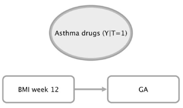
Figure 8: DAG resulting from MMHC, $\widehat{Q}_{\rightarrow T}^{1}$

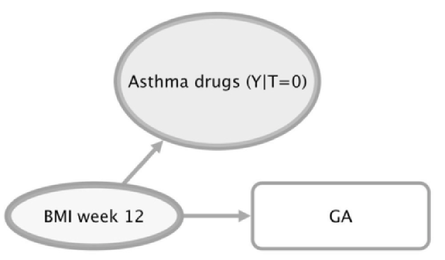
Figure 9: DAG resulting from MMHC, $\widehat{Q}_{\rightarrow T}^{0}$

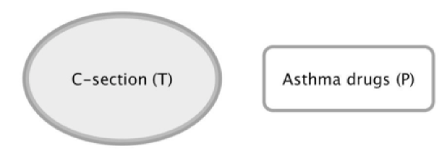
Figure 10: DAG resulting from MMHC, $\widehat{Z}_{\rightarrow Y}^{1}$

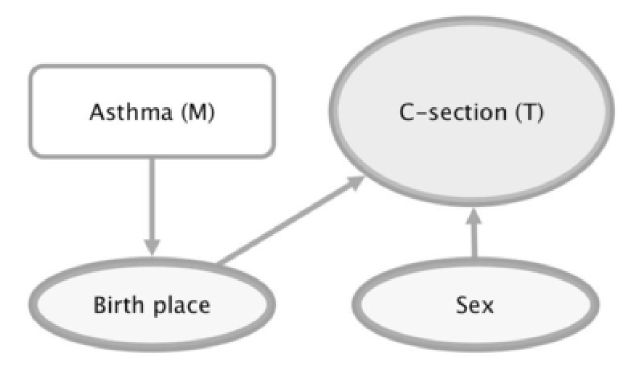
Figure 11: DAG resulting from MMHC, $\widehat{Z}_{\rightarrow Y}^{0}$

References

- Abadie and Imbens (2006) Abadie, A. and Imbens, G. W. (2006). Large sample properties of matching estimators for average treatment effects. Econometrica 74, 235–267.
- Bråbäck et al. (2013) Bråbäck, L., Ekéus, C., Lowe, A. J., and Hjern, A. (2013). Confounding with familial determinants affects the association between mode of delivery and childhood asthma medication–a national cohort study. Allergy, Asthma & Clinical Immunology 9, 1–9.
- Breiman (2001) Breiman, L. (2001). Random forests. Machine Learning 45, 5–32.
- Chickering (2002) Chickering, D. M. (2002). Optimal structure identification with greedy search. Journal of Machine Learning Research 3, 507–554.
- Chipman et al. (2010) Chipman, H. A., George, E. I., and McCulloch, R. E. (2010). BART: Bayesian additive regression trees. The Annals of Applied Statistics 4, 266–298.
- Dawid (1979) Dawid, A. P. (1979). Conditional independence in statistical theory. Journal of the Royal Statistical Society, Series B 41, 1–31.
- de Luna et al. (2011) de Luna, X., Waernbaum, I., and Richardson, T. S. (2011). Covariate selection for the nonparametric estimation of an average treatment effect. Biometrika 98, 861–875.
- Ding and Miratrix (2015) Ding, P. and Miratrix, L. W. (2015). To adjust or not to adjust? Sensitivity analysis of M-bias and Butterfly-bias. Journal of Causal Inference 3, 41–57.
- Friedman et al. (2010) Friedman, J., Hastie, T., and Tibshirani, R. (2010). Regularization paths for generalized linear models via coordinate descent. Journal of Statistical Software 33, 1–22.
- Friedman et al. (1999) Friedman, N., Nachman, I., and Peér, D. (1999). Learning Bayesian network structure from massive datasets: the ”sparse candidate” algorithm. In Proceedings of the Fifteenth conference on Uncertainty in artificial intelligence, pages 206–215. Morgan Kaufmann Publishers Inc.
- Greenland (2003) Greenland, S. (2003). Quantifying biases in causal models: Classical confounding vs collider-stratification bias. Epidemiology 14, 300–306.
- Gruber and van der Laan (2012) Gruber, S. and van der Laan, M. J. (2012). tmle: An R package for targeted maximum likelihood estimation. Journal of Statistical Software 51, 1–35.
- Hill (2011) Hill, J. L. (2011). Bayesian nonparametric modeling for causal inference. Journal of Computational and Graphical Statistics 20, 217–240.
- Häggström (2016) Häggström, J. (2016). CovSelHigh: Model-Free Covariate Selection in High Dimensions. R package version 1.0.0.
- Häggström et al. (2015) Häggström, J., Persson, E., Waernbaum, I., and de Luna, X. (2015). CovSel: An R package for covariate selection when estimating average causal effects. Journal of Statistical Software 68, 1–20.
- Kapelner and Bleich (2016) Kapelner, A. and Bleich, J. (2016). bartMachine: Machine learning with Bayesian additive regression trees. Journal of Statistical Software 70, 1–40.
- King and Nielsen (2016) King, G. and Nielsen, R. (2016). Why propensity scores should not be used for matching. Working paper. Copy at http://j.mp/1sexgVw.
- Liaw and Wiener (2002) Liaw, A. and Wiener, M. (2002). Classification and regression by randomForest. R News 2, 18–22.
- Lindgren et al. (2016) Lindgren, U., Nilsson, K., de Luna, X., and Ivarsson, A. (2016). Data resource profile: Swedish microdata research from childhood into lifelong health and welfare (Umeå SIMSAM Lab). International Journal of Epidemiology 45, 1075–1075g.
- Liu et al. (2012) Liu, W., Brookhart, M. A., Schneeweiss, S., Mi, X., and Setoguchi, S. (2012). Implications of M bias in epidemiologic studies: A simulation study. American Journal of Epidemiology 176, 938–948.
- Maathuis et al. (2009) Maathuis, M. H., Kalisch, M., and Bühlmann, P. (2009). Estimating high-dimensional intervention effects from observational data. The Annals of Statistics 37, 3133–3164.
- Magnus et al. (2011) Magnus, M. C., Håberg, S. E., Stigum, H., Nafstad, P., London, S. J., Vangen, S., and Nystad, W. (2011). Delivery by Cesarean section and early childhood respiratory symptoms and disorders: the Norwegian mother and child cohort study. American Journal of Epidemiology 174, 1275–1285.
- Neyman (1923) Neyman, J. (1923). On the application of probability theory to agricultural experiments, essay on principles. Roczniki nauk Rolczych X, 1-51. In Polish. English translation by D.M. Dabrowska and T.P. Speed in Statistical Science 5, 465–472.
- Pearl (1995) Pearl, J. (1995). Causal diagrams for empirical research. Biometrika 82, 669–688.
- Pearl (2009a) Pearl, J. (2009a). Causality, Second edition. Cambridge University Press, Cambridge.
- Pearl (2009b) Pearl, J. (2009b). Letter to the editor. Statistics in Medicine 28, 1415–1416.
- Persson et al. (2017) Persson, E., Häggström, J., Waernbaum, I., and de Luna, X. (2017). Data-driven algorithms for dimension reduction in causal inference. Computational Statistics & Data Analysis 105, 280–292.
- R Core Team (2016) R Core Team (2016). R: A Language and Environment for Statistical Computing. R Foundation for Statistical Computing, Vienna, Austria.
- Rubin (1974) Rubin, D. B. (1974). Estimating causal effects of treatments in randomized and nonrandomized studies. Journal of Educational Psychology 66, 688–701.
- Rubin (1990) Rubin, D. B. (1990). Formal modes of statistical inference for causal effects. Journal of Statistical Planning and Inference 25, 279–292.
- Rubin (2007) Rubin, D. B. (2007). The design versus the analysis of observational studies for causal effects: Parallels with the design of randomized trials. Statistics in Medicine 26, 20–36.
- Rubin (2008a) Rubin, D. B. (2008a). Author’s reply (to Ian Shrier’s letter to the editor). Statistics in Medicine 27, 2741–2742.
- Rubin (2008b) Rubin, D. B. (2008b). For objective causal inference, design trumps analysis. The Annals of Applied Statistics 2, 808–840.
- Rubin (2009) Rubin, D. B. (2009). Author’s reply (to Judea Pearl’s and Arvid Sjölander’s letters to the editor). Statistics in Medicine 28, 1420–1423.
- Schnitzer et al. (2016) Schnitzer, M. E., Lok, J. J., and Gruber, S. (2016). Variable selection for confounder control, flexible modeling and collaborative targeted minimum loss-based estimation in causal inference. The International Journal of Biostatistics 12, 97–115.
- Scutari (2010) Scutari, M. (2010). Learning Bayesian networks with the bnlearn R package. Journal of Statistical Software 35, 1–22.
- Sekhon (2011) Sekhon, J. S. (2011). Multivariate and propensity score matching software with automated balance optimization: the Matching package for R. Journal of Statistical Software 42, 1–52.
- Shannon et al. (2003) Shannon, P., Markiel, A., Ozier, O., Baliga, N. S., Wang, J. T., Ramage, D., Amin, N., Schwikowski, B., and Ideker, T. (2003). Cytoscape: A software environment for integrated models of biomolecular interaction networks. Genome Research 13, 2498–2504.
- Shrier (2008) Shrier, I. (2008). Letter to the editor. Statistics in Medicine 27, 2740–2741.
- Sjölander (2009) Sjölander, A. (2009). Letter to the editor. Statistics in Medicine 28, 1416–1420.
- Spirtes et al. (2000) Spirtes, P., Glymour, C. N., and Scheines, R. (2000). Causation, Prediction, and Search. MIT press.
- Tibshirani (1996) Tibshirani, R. (1996). Regression shrinkage and selection via the lasso. Journal of the Royal Statistical Society. Series B (Methodological) 58, 267–288.
- Tsamardinos et al. (2006) Tsamardinos, I., Brown, L., and Aliferis, C. (2006). The max-min hill-climbing Bayesian network structure learning algorithm. Machine Learning 65, 31–78.
- van der Laan and Rubin (2006) van der Laan, M. J. and Rubin, D. (2006). Targeted maximum likelihood learning. The International Journal of Biostatistics 2, 1–38.
- VanderWeele and Shpitser (2011) VanderWeele, T. J. and Shpitser, I. (2011). A new criterion for confounder selection. Biometrics 67, 1406–1413.
- WHO Collaborating Centre for Drug Statistics Methodology (2014) WHO Collaborating Centre for Drug Statistics Methodology (2014). ATC Classification Index With DDDs, 2015. WHO Collaborating Centre for Drug Statistics Methodology, Oslo, Norway.