MOCCA code for star cluster simulations – VI. Bimodal spatial distribution of blue stragglers

Abstract

The paper presents an analysis of formation mechanism and properties of spatial distributions of blue stragglers in evolving globular clusters, based on numerical simulations done with the mocca code. First, there are presented N-body and mocca simulations which try to reproduce the simulations presented by Ferraro et al. (2012). Then, the agreement between N-body and the mocca code is shown. Finally, we discuss the formation process of the bimodal distribution. We report that so-called bimodal spatial distribution of blue stragglers is a very transient feature. It is formed for one snapshot in time and it can easily vanish in the next one. Moreover, we show that the radius of avoidance proposed by Ferraro et al. (2012) goes out of sync with the apparent minimum of the bimodal distribution after about two half-mass relaxation times. This finding creates a real challenge for the dynamical clock, which uses this radius to determine the dynamical age of globular clusters. Additionally, the paper discusses a few important problems concerning the apparent visibilities of the bimodal distributions which have to be taken into account while studying the spatial distributions of blue stragglers.

1 Introduction

Blue straggler stars (BSs) are important members of globular clusters (GCs). They are promising tools to study the complex interplay between the dynamical evolution of globular clusters and stellar evolution. BSs are defined as stars which are brighter than the main-sequence (MS) turn-off point (also their mass is larger than the stars on the turn-off point). They lie on the extension of the main-sequence in color-magnitude diagram (CMD). Thus, they had to acquire somehow an additional mass to stay on the main-sequence longer. Two possible channels of their formation involve a physical collision with another star or some mass transfer. BSs were first discovered by Sandage (1953) in M3, later they were observed in essentially all clusters (Piotto et al., 2004). BSs were discovered also in open clusters, e.g. Mathieu & Geller (2009) and dwarf galaxies e.g. Mateo et al. (1995), Mapelli et al. (2007) or Monelli et al. (2012).

In order to study radial positions of BSs in GCs one needs to compare their number as a function of radius with other types of stars which are assumed that they trace the radial density distribution of stars in a cluster. In the literature the best two, from among such candidate populations, are HB stars and RGB stars. Their number is sufficiently high, they are well visible on the CMD, and they are present essentially on any radial distance from the center throughout the entire cluster. Additionally, their lifetimes are rather short, and thus, they are rather unchanged by stellar dynamics significantly during their lifetimes (like more massive BSs). Thus, HB and RGB radial positions trace clusters densities very well.

For a quantitative analysis, GC is divided into a number of concentric annuli around the cluster center and a specific frequency definition is introduced (Ferraro et al., 1993). The specific frequency, called also the double normalized ratio, is defined by the equation:

$$R_{pop}=\frac{N_{pop}/N^{tot}_{pop}}{L_{samp}/L^{tot}_{samp}}$$ (1)

where $pop$ described BSs, HB or RGB stars, $N_{pop}$ is the number of stars of a given population (e.g. $N_{BSS}$), and $N^{tot}_{pop}$ is the total number of stars from a given population. $L_{samp}$ denotes the sampled luminosity measured in each annulus and $N^{tot}_{samp}$ is the total luminosity for all annuli. The luminosity in each annulus is calculated by integrating the single-mass King model that best fits the observed surface density profile (see e.g. Lanzoni et al. (2007)). The reddening, distance to the cluster, and possible incompleteness in spatial coverage of the outermost annuli should be taken into account as well. The specific frequency, $R_{pop}$, is a very useful quantity which allows to show whether the number of stars from a given population shows signs of an increased number in some parts of a GC. The luminosity of GCs is very smooth through out the entire cluster and very well represents ,,underlying” mass of GC. By scaling the number of BSs, or another population, with luminosities, one can compare GCs of various sizes with various dynamical statuses. For example, if the number of BSs was significantly larger in the center of GC, the specific frequency would reveal it with values larger than 1.0. The bimodal, unimodal and flat radial distributions of BSs are nicely visible with the specific frequency (see below).

Ferraro et al. (2003) defined the BSs specific frequency as the number of BSs, normalized to the number of the horizontal branch stars. They examined six GCs and found that the BSs’ specific frequency varies from 0.07 to 0.92, and it does not depend on the central density, total mass, and velocity dispersion. What is surprising, they found the largest BSs specific frequencies for clusters with the lowest central density (NGC 288) and the highest central density (M80). Ferraro et al. (2003) claim that these two kinds of BSs formation processes, i.e., mass transfer and mergers, can have comparable efficiency in producing BSs in their respective typical environments.

Sollima et al. (2008) found a strong correlation between the BSs specific frequency and the linear combination of the binary fraction ($\xi_{bin}$) and velocity dispersion ($\sigma_{v}$): $\xi_{bin}+\alpha\sigma_{v}$, where $\alpha=-4.62$. This indicates that, for a given binary fraction, the BSs specific frequency decreases with increasing velocity dispersion. Small cluster velocity dispersion corresponds to a lower binding energy limit between soft and hard binaries (to a larger fraction of hard binaries). Since the natural evolution of hard binaries leads to an increase of their binding energy (Heggie, 1975), low velocity dispersion GCs should host a larger fraction of hard binaries, which are able to survive both, stellar encounters and activate mass-transfer, and/or merging processes between the companions (Sollima et al., 2008). Therefore, more BSs formed by the evolution of primordial binaries is expected to form in lower velocity dispersion GCs.

The radial distribution of BSs in many clusters is bimodal. First discoveries of bimodal distributions were made for M3 by Ferraro et al. (1993); Ferraro et al. (1997) and by Zaggia et al. (1997) for M55. The BSs radial distribution for the M3 cluster clearly shows a maximum at the center of the cluster, a clear-cut dip in the intermediate region, and again a rise of BSs in the outer region of the cluster (but lower than the central value). The bimodal distribution of BSs was later shown by other authors for other clusters like 47 Tuc (Ferraro et al., 2004), NGC 6752 (Sabbi et al., 2004), M55 (Lanzoni et al., 2007), M5 (Warren et al., 2006; Lanzoni et al., 2007) and others. Sigurdsson et al. (1994) suggested that BSs were formed by direct collisions in the center of the cluster and then ejected to the outer part of the system as a result of a dynamical interaction. Ejected BSs were afterwards moved back to the center of the cluster because of the mass segregation, which leads to the increase of the number of BSs in the center of the system. If dynamical interactions were energetic enough, then BSs would stay outside of the cluster for longer time and this could be the reason why there is a higher rate of formation of BSs in the outer part of the cluster, i.e., the second peak of the BSs in the bimodal distribution. Later, the bimodal distribution of BSs in the cluster was explained differently by Ferraro et al. (1997). They showed it as a result of different processes forming BSs in different parts of the cluster – mass transfer for the outer BSs and stellar collisions leading to mergers for BSs in the center of the cluster. Furthermore, Mapelli et al. (2004a); Mapelli et al. (2006a) and Lanzoni et al. (2007), by performing numerical simulations, showed that the bimodal distribution in the cluster cannot be explained only by a collisional scenario in which BSs are created in the center of the cluster and some of them are ejected to the outer part of the system. This process is believed to be not efficient enough, and $\sim 20-40\%$ of BSs have to be created in the peripherals in order to get the required number of BSs for the cluster. It is believed that in the outer part of a star cluster, binaries can start mass transfer in isolation without suffering from energetic dynamical interactions with field stars. Even if one can observe a bimodal distribution of BSs for many clusters, one can not generalize this feature. There are known clusters for which radial distributions are even flat, like for NGC 2419 (Dalessandro et al., 2008a; Contreras Ramos et al., 2012).

For GCs, which have signs of the bimodal spatial distribution, the radius at the minimum of the specific frequency is called the radius of avoidance ($r_{avoid}$). See Lanzoni et al. (2007, Fig. 12) for a few examples of $r_{avoid}$ in GCs with respect to the GCs core radii. The area surrounding the radius of avoidance is called ,,zone of avoidance” (Mapelli et al., 2004b). The radius of avoidance is a quantitative value which describes the radius below which all heavier objects are expected to have enough time to already sink to the center of GC. BSs are example of such objects. They have masses larger than $m_{turn-off}$, some of them can have masses even close to $2\times m_{turn-off}$ (collisional BSs) – they are significantly larger than the average mas of stars in a GC. Some BSs appear in binaries, which lowers the mass segregation time for them even more. The radius of avoidance is a value which divides the GC essentially into two regions. The structure below the $r_{avoid}$ is expected to be mass-segregated and thus it should not reflect the initial GC properties. More massive objects, like BSs, are expected to be found already in the deep center of the GC ($<r_{c}$). However, the stars at the distances larger than $r_{avoid}$ should more-less resemble the initial GC properties, because at such large radii dynamical processes in GC should not change significantly the structure of the GC. Thus, it is expected e.g. for mass-transfer BSs (EMT), created as a result of unperturbed evolution, to stay more or less on their initial orbits. The radius of avoidance can be calculated from the equation for the dynamical friction time $t_{df}$ by (Binney & Tremaine, 1987):

$$t_{df}=\frac{3}{4~{}ln\Lambda~{}G^{2}~{}(2\Pi)^{0.5}}\frac{\sigma(r)^{3}}{m_{BSS}~{}\rho(r)}$$ (2)

where $ln\Lambda$ is the Coulomb logarithm, G is gravitational constant and $\sigma(r)$, $\rho(r)$ are cluster velocity dispersion and density at the radius $r$. Masses of the BSs are usually assumed to be $m_{BSS}=1.2M_{\odot}$.

NGC 6388 is another example of a very well studied globular cluster in terms of the BSs population and radial properties, see Dalessandro et al. (2008b). They show this bimodal spatial distribution of BSs in NGC 6388 together with a flat distribution of HB (which are used here to trace the entire GC mass distribution). In NGC 6388 several groups of HB stars were recognized. HB referred here is the red-HB (RGH) subgroup – the most numerous group of HB stars characteristic for metal-reach stellar populations (for more details about HB subgroups see Dalessandro et al. (2008b)). The bimodal distribution is clearly visible with its central peak in the cluster center, then a clear fall around $4-5r/r_{c}$, and again an increase of the number of BSs in the outer parts of GCs ($>5r/r_{c}$).

The bimodal radial distribution is also visible in the cumulative plot which very well represents the internal radial structure of the GC (Dalessandro et al., 2008b). It represents the cumulative number of BSs ($\Phi$) and the corresponding cumulative number of HB stars starting from the deep center ($\Phi=0$) of the cluster up to its outer regions ($\Phi=1$). The fraction of BSs is clearly larger in the center ($\Phi\leq 0.5$), which corresponds to the most central $\sim 30^{\prime\prime}$ of the GC. Then, the fraction of HB stars outnumbers the BSs population. The cumulative number of BSs raises again near $100^{\prime\prime}$ of the center of GC. It is worth to notice how smooth the cumulative number of HB stars is, which makes them a very good reference population for the radial positions of BSs.

Dalessandro et al. (2008b) claim that the radial distribution of BSs in NGC 6388 is peculiar. Although it is clearly bimodal (see Dalessandro et al. (2008b, Fig. 11)), BSs occupy regions which already should be cleared from them due to dynamical friction. The position of the radius of avoidance ($r_{avoid}$) for NGC 6388 does not correspond to the dip in the intermediate region, where the number of BSs is the lowest (Dalessandro et al., 2008b). The radius of avoidance, $r_{avoid}\simeq 15r_{c}$, was calculated using Eq. 2, GC age was assumed to be $t_{age}=12$ Gyr, velocity dispersion $\sigma_{0}=18.9km/s$, and stellar density of the order of $10^{6}stars/pc^{3}$ (Pryor & Meylan, 1993). The position of $r_{avoid}$ is rather unexpected. It is about 3 times larger than the dip in the bimodal spatial distribution ($5r_{c}$). This could suggest that the dynamical friction, responsible for creating so-called ,,zone of avoidance”, is not as efficient as it was previously thought. NGC 6388 GC seems to be ,,dynamically younger” than assumed because BSs segregated only up to $5r_{c}$, rather than to the expected $15r_{c}$. Dalessandro et al. (2008b) discuss the possibility of the existence of IMBH in the center of NGC 6388 but it is not clear how it affects GC at radii of about $5-15r_{c}$. Moreover, if IMBH existed in the center of NGC 6388 and BSs were influenced by strong interactions with central objects, then BSs would be ejected to the outer regions but across all radii. The ejected BSs would fill the dip around $5r_{c}$ rather than concentrating in the outskirts of GC. It is especially important from the point of view of this paper, which also suggests that dynamical friction is itself a very interesting explanation, but it does not explain all features observed in the mocca simulations. The picture of formation of bimodal spatial distribution for GCs seems to be more complex (see Section. 3).

Dynamical simulations of Mapelli et al. (2004b, 2006b) and Lanzoni et al. (2007) showed that rather a large number of collisional BSs ($\lesssim 50\%$) is needed to reproduce the number of BSs in the central peak. Additionally, about 20-40% of mass-transfer BSs are needed to reproduce the number of BSs in the outer regions of GCs.

A detail study of BSs radial distribution was performed by Lanzoni et al. (2007) for NGC 1904 (M79). They used wide-field ground based ESO-WFI and space GALEX observations to collect a multiwavelength photometric data (from far UV to near infrared). What is important, this extensive work covered entire cluster extension from the very central regions up to the tidal radius. In total, position of 39 BSs were analyzed and they have been found to be highly segregated in the cluster core. No other increase of the number of BSs were found in the outskirts of GC. No evidence for the bimodal spatial distribution in this case is consistent with the formation mechanism based on the dynamical friction which drives BSs into the center of the GC. In the Harris catalogue (Harris, 1996) NGC 1904 is denoted as core-collapsed GC and thus stars in this GC are most probably already fully segregated and there is no expectation to observe the bimodal spatial distribution. Radius of avoidance for NGC 1904 is $r_{avoid}\sim 30r_{c}$ (see Eq. 2) which supports the conclusions of the fully mass segregation of this GC (Lanzoni et al., 2007).

For the GC $\omega$ Cen the radial distribution of BSs is flat (Ferraro et al., 2006). This GC is simply too large and mass segregation processes did not have enough time to alter the BSs positions. There is no increase in the number of BSs in the center and there is no evidence of the second peak in the outskirts of GC.

Blue stragglers are luminous stars in GCs and thus they are useful to probe the dynamical evolution of stellar systems. Ferraro et al. (2012) used them to build a dynamical clock of GCs. Using their location inside GCs, they tried to infer the dynamical stage reached by GCs. They suggest that the only physical mechanism which lies behind such a clock is the dynamical friction.

At the end of the introductory section it is worth to mention that in the literature, terms collision and merger are used differently by different authors. In this paper the term collision is defined as a physical collision between at least two stars during a dynamical interaction, while the term merger is defined as a coalescence between stars from one binary as a result of stellar evolution.

This paper is organized as follows. The Sect. 2 briefly describes the properties of various models computed for the needs of this work. In the Sect. 3 there is detailed analysis of the formation and evolution of the bimodal spatial distribution of BSs. First, we described an attempt to reproduce available N-body simulations, then we present comparison between our N-body simulations and mocca code simulations. Finally, in this section we discuss in details the formation mechanism of the bimodal spatial distribution for real-size GCs. In the Sect.4 we summarize or work and discuss its influence on the observations of GCs.

2 Numerical simulations

The numerical simulations were performed with the mocca code (Hypki & Giersz, 2013).

The mocca code is one of the most advanced codes to simulate real size globular clusters and provide full information on the stellar and dynamical evolution of all stars in such system. It originates from the Monte Carlo code for star clusters simulations developed by Hénon (1971), then improved by Stodolkiewicz (1986) and later heavily developed by Giersz and collaborators (Giersz et al., 2013, 2015). The stellar evolution is done for both single and binary stars using SSE and BSE codes (Hurley et al., 2000, 2002). Recently, the Monte Carlo code was integrated with fewbody code of Fregeau & Rasio (2007) to deal with strong interactions like in N-body codes. The code got a new name – mocca. This addition allows the mocca code to follow the formation and evolution of exotic objects, for instance blue stragglers (Hypki & Giersz, 2013).

2.1 Initial parameters for the mocca code simulations

The mocca code was used to compute many models of globular clusters with various initial conditions. The models and their properties are summarized in Tab. 1 and Tab. 2.

The models from Tab. 1 and Tab. 2 are identical to the models presented in another paper in the series about BSs (Hypki et al. 2016, MOCCA code for star cluster simulations – V. Initial globular cluster conditions influence on blue stragglers, submitted). This other paper shows how various initial conditions of globular clusters and various initial properties of binaries influence the population of BSs. The copy of Tab. 1 and Tab. 2 is however left in this paper for the sake of completeness.

initial mass function of the mocca simulations (Part I)
Name	$N$	$f_{b}$	IM	$IMF_{s}$	$IMF_{b}$	q	a	e	z	$r_{tid}$	$r_{h}$
mocca-1	300k	0.1	P	K93	K91	U	UL	T	0.001	69	6.9
mocca-2	300k	0.2	P	K93	K91	U	UL	T	0.001	15	1.5
mocca-3	300k	0.2	P	K93	K91	U	UL	T	0.001	25	2.5
mocca-4	300k	0.2	P	K93	K91	U	UL	T	0.001	35	3.5
mocca-5	300k	0.2	P	K93	K91	U	UL	T	0.001	45	4.5
mocca-6	300k	0.2	P	K93	K91	U	UL	T	0.001	69	1.2
mocca-7	300k	0.2	P	K93	K91	U	UL	T	0.001	69	1.7
mocca-8	300k	0.2	P	K93	K91	U	UL	T	0.001	69	2.3
mocca-9	300k	0.2	P	K93	K91	U	UL	T	0.001	69	2.8
mocca-10	300k	0.2	P	K93	K91	U	UL	T	0.001	69	3.5
mocca-11	300k	0.2	P	K93	K91	U	UL	T	0.001	69	4.6
mocca-12	300k	0.2	P	K93	K91	U	UL	T	0.001	69	6.9
mocca-13	300k	0.2	P	K93	K91	U	UL	T	0.001	69	9.9
mocca-14	300k	0.2	P	K93	K91	U	UL	T	0.001	69	17.3
mocca-15	300k	0.2	P	K93	K91	U	UL	T	0.001	85	8.5
mocca-16	300k	0.2	P	K93	K91	U	UL	T	0.001	135	13.5
mocca-17	300k	0.2	P	K93	K91	U	UL	T	0.001	235	23.5
mocca-18	300k	0.2	P	K93	K91	U	UL	T	0.001	335	33.5
mocca-19	300k	0.3	P	K93	K91	U	UL	T	0.001	69	9.6
mocca-20	300k	0.5	P	K93	K91	U	UL	T	0.001	69	9.6
mocca-21	600k	0.05	P	K93	K91	U	UL	T	0.001	100	10.0
mocca-22	600k	0.1	P	K93	K91	U	UL	T	0.001	100	10.0
mocca-23	600k	0.2	P	K93	K91	U	UL	T	0.001	25	2.5
mocca-24	600k	0.2	P	K93	K91	U	UL	T	0.001	35	0.9
mocca-25	600k	0.2	P	K93	K91	U	UL	T	0.001	35	1.2
mocca-26	600k	0.2	P	K93	K91	U	UL	T	0.001	35	1.8
mocca-27	600k	0.2	P	K93	K91	U	UL	T	0.001	35	3.5
mocca-28	600k	0.2	P	K93	K91	U	UL	T	0.001	55	1.4
mocca-29	600k	0.2	P	K93	K91	U	UL	T	0.001	55	1.8
mocca-30	600k	0.2	P	K93	K91	U	UL	T	0.001	55	2.8
mocca-31	600k	0.2	P	K93	K91	U	UL	T	0.001	55	5.5
mocca-32	600k	0.2	P	K93	K91	U	UL	T	0.001	100	1.7
mocca-33	600k	0.2	P	K93	K91	U	UL	T	0.001	100	2.5
mocca-34	600k	0.2	P	K93	K91	U	UL	T	0.001	100	5.0
mocca-35	600k	0.2	P	K93	K91	U	UL	T	0.001	100	10.0
mocca-36	600k	0.2	P	K93	K91	U	UL	T	0.001	100	20.0
mocca-37	600k	0.2	P	K93	K91	U	UL	T	0.001	180	18.0
mocca-38	600k	0.2	P	K93	K91	U	UL	T	0.001	130	13.0
mocca-39	600k	0.2	P	K93	K91	U	UL	T	0.001	230	23.0
mocca-40	600k	0.2	P	K93	K91	U	UL	T	0.001	300	30.0
mocca-41	600k	0.2	P	K93	K91	U	UL	T	0.001	400	40.0
mocca-42	600k	0.4	P	K93	K91	U	UL	T	0.001	100	10.0
mocca-43	600k	0.5	P	K93	K91	U	UL	T	0.001	100	10.0

Table 1: Initial conditions of mocca simulations done for the purpose of this paper. Symbols have the following meaning: N – initial number of objects (single + binary stars), $f_{b}$ – initial binary fraction, $f_{b}=N_{b}/N$ ($N_{b}$ – number of binaries), $IM$ – initial model, P – Plummer model, $IMF_{s}$ – Initial Mass Function for single stars, K93 – Kroupa et al. (1993) in the range $[0.1;100]\mathrm{M_{\odot}}$, $IMF_{b}$ – Initial Mass Function for binary stars, K91 – Kroupa et al. (1991, eq. 1), binary masses from 0.2 to 100 $\mathrm{M_{\odot}}$, q – distribution of mass ratios between stars in binaries, U – uniform distribution of mass ratios, R – random pairing of masses for binary components, a – semi-major axes distribution, UL – uniform distribution of semi-major axes in the logarithmic scale from $2(R_{1}+R_{2})$ to 100 AU, L – lognormal distribution of semi-major axes from $2(R_{1}+R_{2})$ to 100 AU, K95 – binary period distribution from Kroupa (1995), K95E – distribution of semi-major axes with eigenevolution and feeding algorithm (Kroupa, 1995), K13 – new eigenevolution and feeding algorithm (Kroupa et al., 2013), e – eccentricity distribution, T – thermal eccentricity distribution, TE – thermal eccentricity distribution with eigenevolution, z – mettalicity (e.g. 0.001 = 1/20 of the solar metallicity 0.02), $r_{tid}$ – tidal radius in pc, $r_{h}$ – half-mass radius in pc. The main difference in the simulation from mocca-1 to mocca-43 is in the dynamical timescales of GCs’ evolution.

initial mass function of the mocca simulations (Part I)
Name	$N$	$f_{b}$	IM	$IMF_{s}$	$IMF_{b}$	q	a	e	z	$r_{tid}$	$r_{h}$
mocca-44	300k	0.2	P	K93	K91	R	UL	T	0.001	69	6.9
mocca-45	300k	0.2	P	K93	K91	R	L	T	0.001	69	6.9
mocca-46	300k	0.2	P	K93	K91	R	K95	T	0.001	69	6.9
mocca-47	300k	0.2	P	K93	K91	R	K95E	T	0.001	69	6.9
mocca-48	300k	0.2	P	K93	K91	R	K13	T	0.001	69	6.9
mocca-49	300k	0.2	P	K93	K91	R	UL	TE	0.001	69	6.9
mocca-50	300k	0.2	P	K93	K91	R	L	TE	0.001	69	6.9
mocca-51	300k	0.2	P	K93	K91	R	K95	TE	0.001	69	6.9
mocca-52	300k	0.2	P	K93	K91	R	K95E	TE	0.001	69	6.9
mocca-53	300k	0.2	P	K93	K91	R	K13	TE	0.001	69	6.9
mocca-54	300k	0.2	P	K93	K91	U	L	T	0.001	69	6.9
mocca-55	300k	0.2	P	K93	K91	U	K95	T	0.001	69	6.9
mocca-56	300k	0.2	P	K93	K91	U	K95E	T	0.001	69	6.9
mocca-57	300k	0.2	P	K93	K91	U	K13	T	0.001	69	6.9
mocca-58	300k	0.2	P	K93	K91	U	UL	TE	0.001	69	6.9
mocca-59	300k	0.2	P	K93	K91	U	L	TE	0.001	69	6.9
mocca-60	300k	0.2	P	K93	K91	U	K95	TE	0.001	69	6.9
mocca-61	300k	0.2	P	K93	K91	U	K95E	TE	0.001	69	6.9
mocca-62	300k	0.2	P	K93	K91	U	K13	TE	0.001	69	6.9
mocca-63	600k	0.2	P	K93	K91	U	K13	TE	0.001	55	5.5

Table 2: For description see Tab. 1

The models from mocca-1 up to mocca-43 (Tab. 1) differ mainly in the dynamical scales of their evolution. These are models which have mainly different tidal radii (distance from the host galaxy) and different concentrations. These are the parameters which are expected to have the biggest influence on the spatial evolution of BSs. They cover the models from slowly evolving ones to the models which evolve very fast and dissolve very quickly (even in several Gyr). Whereas, the models with identifiers larger than 43 (Tab. 2) differ mainly in the initial parameters of binaries (e.g. different initial semi-major axes distributions, eccentricity distributions). They were used mostly in the already mentioned other paper about BSs. Nevertheless, they were also used in this paper to check whether the different initial binaries properties could have some additional influence on the formation of the bimodal spatial distribution of blue stragglers.

All models from Tab. 1 and Tab. 2 were used to study the evolution of the spatial distribution of BSs in evolving globular clusters. However, eventually we have carefully chosen only three models to support the conclusions of this work (see Sect. 3.2).

The core radius ($r_{c}$) referred in this work is computed with Casertano & Hut (1985), the relaxation time ($t_{rh}$) is actually the half-mass relaxation time (unless noted otherwise) and a star is considered as the blue straggler in mocca simulations if it exceeds the turn-off mass by at leas 2% (for details see Hypki & Giersz (2013)).

3 Bimodal spatial distribution of blue stragglers

This section presents a study of the spatial distribution of blue stragglers in GCs. For a few of them the bimodal distribution is observed (see Sect. 1). In the first subsection we present a comparison between N-body and mocca simulations in terms of the spatial distribution of blue stragglers. We show that the mocca code is a suitable tool to track positions of BSs in stellar systems. The next subsection shows the formation and evolution of the bimodal spatial distribution for the real-size star clusters. This subsection points out also its important implications on the determination of the dynamical ages of GCs.

3.1 N-body and MOCCA simulations of simplified models

The origin and evolution of the bimodal spatial distribution in the simulations done with the mocca code for real-size star clusters was very challenging from the beginning. It was very difficult to obtain clear signs of the bimodality of blue stragglers. Moreover, the bimodal distribution appeared to be very transient. It was present for some snapshots in time and then after one or several next snapshots ($\sim$ hundreds of Myr) the signs of bimodality disappeared. It was very difficult to recreate observations or results from the N-body simulations presented already in the literature (Ferraro et al., 2012). Thus, we decided to perform a series of sanity checks and comparisons with N-body models. The results of these tests are presented here. They should give a proper confidence to the results obtained by the mocca code for simulations of real-size star clusters presented and discussed in Sect. 3.2.

Simulations which show the formation of bimodal spatial distribution were performed by Ferraro et al. (2012) with nbody6 code (Aarseth, 2003; Nitadori & Aarseth, 2012). The results of the simulations are shown in Ferraro et al. (2012, Supplementary Fig. 2). They performed 8 N-body simulations with 16k particles. For each simulation 3 projections of stars’ positions to the plane of the sky were made along three main axes to have a better statistics. The initial conditions for simulations were simplified. Each simulation consisted initially only of stars with three different masses: 1% of heavy BSs with masses $1.2M_{\odot}$, 10% of RGB stars with masses $0.8M_{\odot}$ and 89% of MS stars with masses $0.4M_{\odot}$. The initial model was a King model with $W_{0}=6$, which corresponds to the concentration $c=r_{tid}/r_{c}\cong 18$. The stellar evolution was switched off, there were no primordial binaries and there was no initial mass segregation present in the system. The simplified initial conditions were chosen to have a very simple physics in the system but with all needed processes essential to form the bimodal spatial distribution of BSs. The values on Y axis are the relative frequency of BSs normalized to the number of RGB stars ($R_{BSS}(r)=[N_{BSS}(r)/N_{BSS,tot}]/[N_{RGB}(r)/N_{RGB,tot}]$). The values on X axis are distances from the center of star cluster in the units of current cluster core radius. The gray strip around unity is drawn for the reference and by definition it represents regions of star cluster in which stars were not yet fully affected by the mass segregation – thus, the relative number between BSs and RGB stars is $\sim 1$. The error bars are calculated based on Poisson counting statistics. The N-body simulations done by Ferraro et al. (2012) are referred in this paper as ff simulations.

The ff simulations show the drift of $r_{min}$, denoted with arrows, from the very center to the outskirts of the star cluster with increasing relaxation time. The radius $r_{min}$ is roughly the position around which the bimodal distribution is visible (roughly the lowest value of $R_{BSS}$). The width of the dip around $r_{min}$ is also increasing with time. Note that the minima $r_{min}$ for all snapshots except $t=0$ reach very low values $\sim 0.1$ $R_{BSS}$. The purpose of these simulations was to show the ongoing evolution of $r_{min}$ due to the mass segregation in the system. Ferraro et al. (2012) used these simulations to show that the physical process behind the formation of the bimodal spatial distribution of BSs is the mass segregation. These simulations were not intended to be compared with any observational data.

Our goal was to try to reproduce ff simulations done by Ferraro et al. (2012) and to verify the mass segregation as the formation process of the bimodal distributions in GCs. First, a number of tests were performed with the nbody6 and the mocca codes to show that there is an agreement between them.

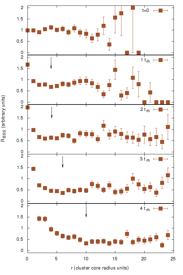
Figure 1: The relative frequency of BSs obtained from direct N-body simulations as an attempt to reproduce results from Ferraro et al. (2012). These are simulations which are referred to as dh simulations in the text. The initial conditions for N-body models are the same as for the simulation showed in Ferraro et al. (2012). The positions of $r_{min}$, chosen by eye, are denoted with arrows. For later times ($>2t_{rh}$) an estimation of the position of $r_{min}$ is rather debatable. However, the overall drift of $r_{min}$ with time should be well visible with the arrows.

The N-body simulations, performed for the purpose of this paper, were done with the same initial conditions as for N-body simulation done by Ferraro et al. (2012) and with the same numerical code, i.e., nbody6. In total, there were made 8 N-body simulations (with 3 projections). They are referred here as dh simulations. They were calculated until the core collapse only ($\sim 5t_{rh}$). The snapshots with the drift or $r_{min}$ value for a few dynamical times ($1,2,3,4t_{rh}$) are presented in Fig. 1. Values for $R_{BSS}$ were calculated in the same way as for ff simulations. The error bars are calculated based on Poisson counting statistics ($R_{BSS}/\sqrt{n_{BSS}}$). The drift is denoted with the arrows and their places were chosen by eye (taking into account error bars). The $r_{min}$ is moving to the outer regions of star cluster with time. This is in agreement with the results of ff simulations.

However, dh simulations were not able to reproduce fully the results obtained by ff simulations (Ferraro et al., 2012). In ff simulations the minimum around $r_{min}$ reaches values of $R_{BSS}\sim 0.2$. These results were unable to reproduce such a large dip around $r_{min}$ for any of the times ($1,2,3,4t_{rh}$, see Fig. 1).

The large differences between ff and dh simulations concern different binning. In Ferraro et al. (2012) the widths of bins are different for different distances from the center of the star cluster. In the dh simulations the width of bins were the same across all distances (in cluster core units). The bins have the same size in order to have a clear picture of the formation and evolution of the $r_{min}$ radius, since variable sizes for bins would introduce only artificial changes of the radial distribution of BSs. The careful selection of the sizes of bins can have a large impact of the visible appearance of the bimodal spatial distributions (see discussion in Sect. 3.3). Interestingly, for the first bin for time $4~{}t_{rh}$ the value for $R_{BSS}$ runs out of the scale already.

Noticeable differences between ff and dh are also in terms of the noise (error bars). ff simulations do not show all bins – e.g. it is not possible that for $t=0$ there are no BSs stars outside $\sim 6r_{c}$ (see Ferraro et al. (2012, Supplementary Fig. 2)). Thus, it is difficult to realize what the noise in the outer regions of star clusters is (after $r_{min}$). However, based on the dh simulations one can see that the noise is very large. The error bars are largest for the bins which are outside $r_{min}$ due to a small number of BSs there.

For the dh simulations there are plotted all 25 first bins, regardless of how many BSs are present in the bin. We decided to have the same sizes for all bins to avoid adding any artificial changes to the signs of bimodal spatial distribution. Together with large errors, the values for $R_{BSS}$ scatter a lot too. Even for time $t=0.0$ many values are not around 1.0 – this is the expected value for non-segregated regions of the star cluster. In the case of ff simulations such errors are not discussed.

However, the overall drift of $r_{min}$ was reproduced in dh simulations but without such a clear minimum around $r_{min}$, like in ff simulations. In the ff model for time $t=2t_{rh}$ it reaches values $R_{BSS}\sim 0.2$, and after $r_{min}$ it raises to values $\sim 1.0$. In the dh model the values are $\sim 0.5$ and in general do not raise to value $\sim 1.0$ after $r_{min}$. This is also the reason why the proper selection of the $r_{min}$ was so difficult.

The positions of $r_{min}$ in the units of the core radii were not reproduced. The radii $r_{min}$ in Ferraro et al. (2012) are significantly further away from the center than in dh simulations. For the time $2t_{rh}$ ff simulation has $r_{min}\sim 10[r/r_{c}]$, whereas in dh simulations $r_{min}$ is about two times smaller ($r_{min}\sim 5[r/r_{c}]$).

The mocca simulation showing the drift of $r_{min}$ is presented in Fig. 2 and it is called ah simulation. The model is essentially the same as for ff and dh simulations with the only difference that for ah simulation the initial number was 100k stars. Thus, the total number of BSs, RGB and MS stars is essentially the same as for ff and dh simulations (8 simulations $\times$ 16k $\sim$ 128k). All the other parameters for ah simulation are the same and the overall evolution between models is very similar as well (e.g. the core collapse for dh and ah models in the units of $t_{rh}$ is the same). The positions of $r_{min}$ are chosen by eye too.

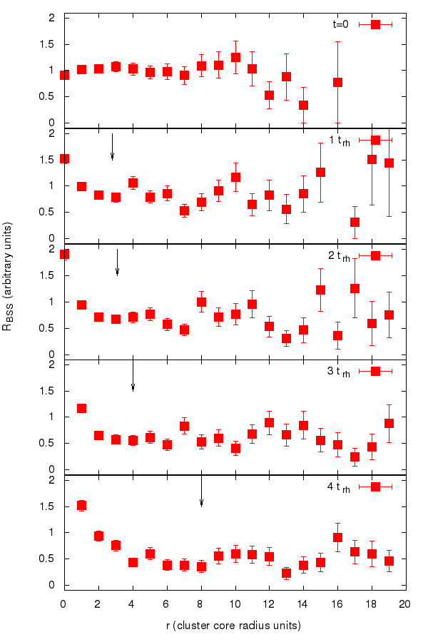
Figure 2: BSs radial distributions obtained from the mocca simulation as an attempt to reproduce the $r_{min}$ drift showed by Ferraro et al. (2012) – this simulation is referred in the text as ah simulation. Its initial conditions are the same as for ff and dh simulations (see Ferraro et al. (2012, Supplementary Fig. 2) and Fig. 1) with the exception that there was made only one mocca simulation but with 100k initial stars (see details in the text). The positions $r_{min}$, chosen by eye, are denoted with arrows. For later times ($>2t_{rh}$) the proper estimation on the location of $r_{min}$ is very debatable. However, the overall drift of $r_{min}$ with time should be well visible with the arrows.

The drift of $r_{min}$ is reproduced in the ah simulation too. Additionally, the dip around $r_{min}$ is also not as significant as in ff simulations – the results are more consistent actually with dh models. The noise in the outer regions is as large as in dh simulations and also the values of $r_{min}$ are different than in ff simulations. These values are, in turn, more consistent with dh simulations.

Large errors for bins outside the $r_{min}$ were the reason to check carefully how the noise really looks like for all snapshots throughout the whole simulation. Fig. 3 shows the radial distribution of normalized number of BSs ($R_{BSS}$) for the 1st, 3rd, 6th and 10th bin for all snapshots. The top panel is for dh simulations, and the bottom one for ah simulation. In other words, Fig. 3 is like Fig. 1, only for selected bins and for all snapshots. Initial parameters for both types of simulations are discussed in the text. The time of the simulation on the X axis is scaled to the core collapse units – in this way it is easier to compare the simulations. The snapshots for ah simulation are performed less frequently, thus, there is less points for it. The first bin for ah simulation has slightly larger values than for dh simulation. It means that for the mocca code there is a slightly larger mass segregation rate. It is a consequence of the larger number of stars for ah simulations (core collapses more significantly for GCs with higher numbers of stars). However, this is not important in the context of the bimodal distribution formation.

The overall trend in Fig. 3 is well visible for both types of simulations. The most central bin constantly increases up to the value $\sim 2.0$. It is caused by the increasing number of BSs in the central region. The 3rd and 6th bins constantly decrease, which corresponds to the continuous decrease of the region around $r_{min}$. The 10th bin remains more or less constant but it has a very large dispersion. The values for $R_{BSS}$, for bins $>1st$, scatter for both simulations significantly. The values for 3rd and 6th bins are alternately smaller and larger with respect to each other. The overall trend is well visible but differences between consequent snapshots are huge. It covers up the signs of bimodal spatial distribution between consequent snapshots. The purpose of this figure is twofold. First of all, it shows that the agreement between N-body dh simulations and mocca ah simulation is good. It shows that the mocca code properly deals with the mass segregation process and thus it is a suitable tool to study radial distribution of exotic objects like BSs. The second goal was to show how greatly chaotic bins are for all snapshots in time, for bins outside the central 1st bin.

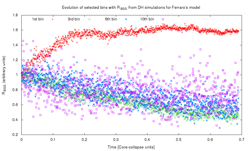
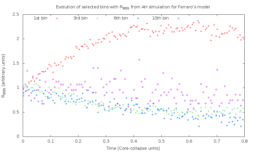
Figure 3: The values of normalized number of BSs ($R_{BSS}$) for the 1st, 3rd, 6th and 10th bins for all snapshots for dh (top) and ah simulations (bottom). Initial parameters are discussed in the text. The time of the simulation on the X axis is scaled to the core collapse units. The snapshots for ah simulation are performed less frequently, thus, there are much less points for the bottom plot. The first bin for ah simulation has a slightly larger value than for dh simulation. However, the overall trend agrees and is well visible for both simulations. The values for $R_{BSS}$ scatter for both simulations significantly (except the 1st bin).

The signs of bimodal spatial distribution for the simplified model defined by Ferraro et al. (2012) is very chaotic both for N-body (dh) and mocca (ah) simulations. Thus, we decided to check the signs of the bimodal distribution for even a simpler model with only two test masses: 99% of MS stars with $0.4M_{\odot}$ and 1% of BSs stars with $1.2M_{\odot}$. This model is called ah2 simulation. All other initial conditions for simulation ah2 are the same as for the ah simulation. Thus, the model ah2 is the simplest possible, for which the mass segregation works only for 2 different masses. The goal was to check whether the signs of the bimodal spatial distributions will be easier to see in comparison to ah simulation (with 3 different masses). The scaling of the normalized number of BSs ($R_{BSS}$) for ah2 model is done with luminosities (there are no RGB stars there).

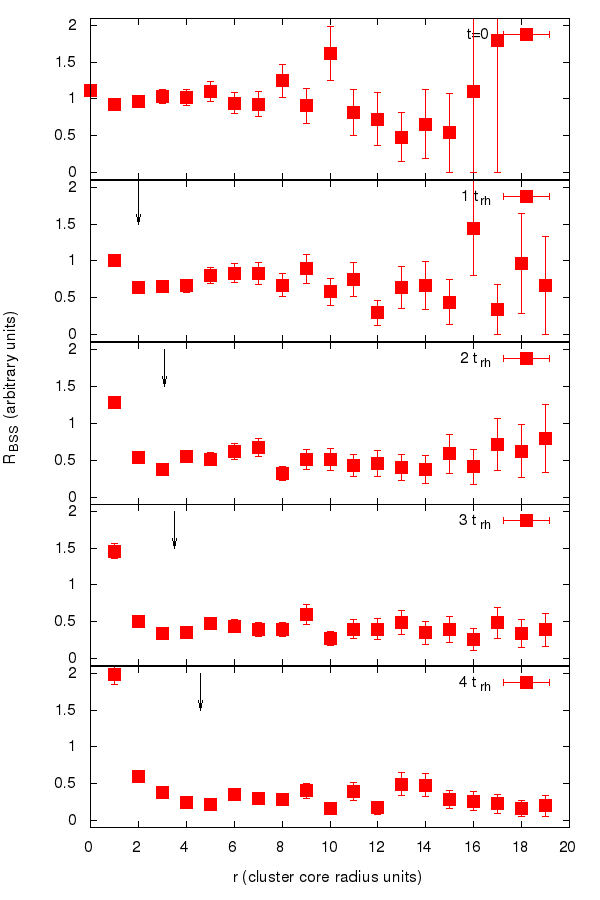
Figure 4: BSS radial distributions of BSs ($R_{BSS}$) obtained from the mocca simulation as an attempt to reproduce $r_{min}$ drift showed by Ferraro et al. (2012) but for the simplified model consisting of only 2 masses: 99% of MS stars with $0.4M_{\odot}$ and 1% of BSs with $1.2M_{\odot}$.

The results for a few half-mass relaxation times for ah2 simulation are presented in Fig. 4. It shows the formation and evolution of the dip around $r_{min}$ value. The minima turned out to be hardly visible, even more difficult than for the ah simulation. The signs of the bimodal spatial distribution are chaotic too. The differences between consequent snapshots are significant – the sign of bimodality can disappear between two following snapshots in time. Even for the simplest possible model, the signs of bimodal distribution are very hard to observe. Thus, for the real-size star cluster the signs of bimodality are expected to be very chaotic, i.e., present for some snapshot and vanishing within the next one or more snapshots.

Another significant difference between ff simulations and dh, ah, ah2 simulations concerns the average value of $R_{BSS}$ outside the $r_{min}$ values. It decreases with time. However, we expected to see them more or less around the value 1.0. The $R_{BSS}\sim 1.0$ is the expected value for the regions which are not yet affected much by the mass segregation (due to larger distances from the center of star cluster). This feature was looked for in ff simulations in order to find the $r_{min}$. However, the values of $R_{BSS}$ are constantly decreasing with time for all of the dh, ah, ah2 simulations (see Fig. 1, Fig. 2, Fig. 4). This constant decrease is likely to originate from the fact that some of BSs move to the cluster’s center faster than the local mass-segregation time. If it happens by a chance that a star (on elongated orbit), while moving through the pericenter of its orbit, will have a close two-body interaction, it may loose more energy and sink to the center more quickly. Nevertheless, dh, ah, ah2 simulations showed that it is rather a wrong assumption to expect the $R_{BSS}$ values to stay at $\sim 1.0$ outside the $r_{min}$.

The comparison between dh and ah simulations shows that the mocca code can follow the mass segregation and thus the changes in positions of BSs as accurately as N-body codes. Thus, the mocca code is a proper tool to study the formation and evolution of the bimodal spatial distribution for real-size stars clusters.

3.2 Bimodal distribution for real-size globular clusters

Three selected models, showing the formation and evolution of the spatial distribution of BSs, were chosen to have different relaxation times and thus different rates of mass segregations. Tab. 3 summarizes the initial parameters for them. The only differences between the models are in the concentrations and the tidal radii. Thus, their rate of the dynamical evolution varies. The slowest evolving model, mocca-slow, has large tidal radius $r_{tid}=180$ [pc], and small concentration $c=r_{tid}/r_{h}=10$. The GC with slightly faster dynamical evolution, mocca-medium, has smaller tidal radius $r_{tid}=100$ [pc], and larger concentration $c=20$. The fastest evolving GC, mocca-fast, has even smaller tidal radius $r_{tid}=55$ [pc] with the same concentration $c=20$. All simulations were computed up to 20 Gyr. The implications of the different rate of evolution of GCs on the population of BSs are presented in Fig. 5 and Fig. 6. The selected models are actually equivalent to models presented in Sect. 2.1, but they are renamed in this section for the sake of clarity. Model mocca-slow is equal to model mocca-37, mocca-medium to mocca-34 and mocca-fast to mocca-30.

Parameter	mocca-slow	mocca-medium	mocca-fast
Single stars ($N_{s}$)	480k
Binary stars ($N_{b}$)	120k
Binary fraction ($f_{b}=\frac{N_{s}}{N_{b}+N_{s}}$)	0.2
Initial model	Plummer
IMF of stars	Kroupa et al. (1993) in the range $[0.1;100]\mathrm{M_{\odot}}$
IMF of binaries	Kroupa et al. (1991, eq. 1), binary masses from 0.2 to 100 $\mathrm{M_{\odot}}$
Total mass (M(0))	$3.4\times 10^{5}\mathrm{M_{\odot}}$
Binary mass ratios	Uniform
Binary semi-major axes	Uniform in the logarithmic scale from $2(R_{1}+R_{2})$ to 100 AU
Binary eccentricities	Thermal (modified by Hurley et al. (2005, eq. 1))
Metallicity	0.001 (1/20 of the solar metallicity 0.02)
Initial tidal radius ($r_{tid}$)	180 pc	100 pc	55 pc
Initial half-mass radius ($r_{h}$)	18 pc	5 pc	2.75 pc
Initial core radius ($r_{c}$)	8.2 pc	3.8 pc	2.0 pc

Table 3: Initial conditions for mocca-slow, mocca-medium and mocca-fast simulations. They represent slowly, slightly faster and fast evolving GCs. Such models were chosen to have different rates of dynamical evolution to study the different speeds of formation and evolution of the bimodal spatial distribution in the real-size GCs. See details in Sect. 3.2.

The first column in Fig. 5 presents the evolution of characteristic radii for the mocca-slow, mocca-medium and mocca-fast simulations. Each plot contains core radius $r_{c}$, half-mass radius $r_{h}$, tidal radius $r_{tid}$, and two additional Lagrangian radii, $r_{1\%}$ and $r_{70\%}$. The changes in radii show the dynamical evolution of the models. For the mocca-slow simulation there are actually no changes of the inner most radii which means that this GC is not affected by the dynamical interactions much. Its evolution is driven mainly by stellar evolution. The faster evolving model, mocca-medium, shows changes in the $r_{1\%}$ and $r_{c}$. The radii get smaller with time, which means that the density increases in the core region of the GC. The fastest evolving GC, mocca-fast, gets even denser and around 16 Gyr one can see the sign of the core collapse in $r_{c}$ – it gets dynamically old.

The second column in the Fig. 5 shows the number of BSs of different types as a function of time for the mocca-slow, mocca-medium and mocca-fast simulations. The number of EM and EMT changes similarly for all three simulations. It is a consequence of the same initial parameters for binaries for the three models. EM and EMT channels in general are not affected by dynamical interactions, thus their numbers are essentially the same for the models with different densities but with the same initial mass functions. The differences in the GCs’ densities have a great influence on the dynamically created BSs (CBS, CBB). Their number differ a lot between the models. The densest and fastest evolving model, mocca-fast, has the largest number of them because of the more frequent strong dynamical interactions between stars which lead to the BSs creation. mocca-fast has also the highest number of BSs which had some interactions with other binaries and changed their companions (EXBS, EXBB) or were disrupted (DBS, DBB). For the details about the formation processes of BSs see Hypki & Giersz (2013).

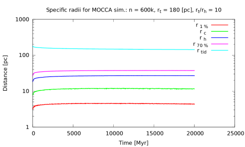
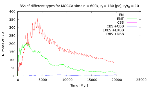
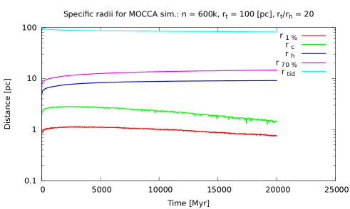
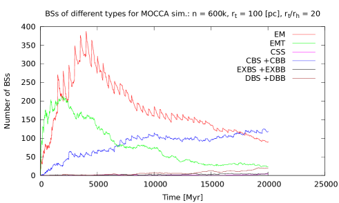
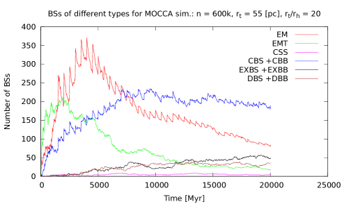
Figure 5: Characteristic radii and number of BSs of different types for mocca-slow (top row), mocca-medium (middle row) and mocca-fast simulations (bottom row). The first column presents a few specific radii as a function of time, like core radius ($r_{c}$), half-mass radius ($r_{h}$), tidal radius ($t_{tid}$), and some Lagrangian radii. The second column shows the number of BSs of different types: EM – evolutionary mergers, EMT – evolution mass transfer, CBS/CBB – collisional binary-single, binary-binary, EXBS/EXBB – exchanged binary-single, binary-binary, and DBS/DBB – dissolved binary-single, binary-binary. For the initial conditions of the models see Tab. 3 and for the discussion of the plots see Sect. 3.2.

Fig. 6 shows the timescales of the GCs evolution which are relevant for the formation of the signs of the bimodal spatial distributions. The first column in Fig. 6 shows the half-mass relaxation times ($t_{rh}$) for the mocca-slow, mocca-medium and mocca-fast models. The $t_{rh}$ is the largest for slowest evolving model and is much larger than the age of the Universe. Whereas the $t_{rh}$ increases for mocca-fast models to only about 3 Gyr after the first few Gyr of the simulation, which is much less than the Hubble time. The second column of Fig. 6 presents the mass-segregation times for 12 Gyr snapshot for BSs, RGB and MS stars. The mass-segregation time gives an impression on how much time is needed for a star at a distance r to sink to the center of GC. For most massive stars, BSs, the times are lowest. The RGB stars, with masses just slightly smaller than these of BSs, have the mass-segregation times only slightly larger. The violet line which denotes 12 Gyr is plotted for a reference to show which portion of stars could be affected already by the mass-segregation process. For the mocca-slow one can see that almost all BSs and RGB stars are above this 12 Gyr limit. Whereas for mocca-fast almost all BSs are well below 12 Gyr.

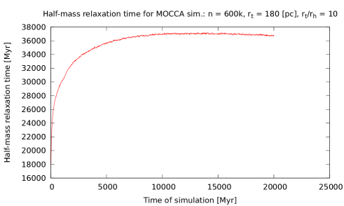
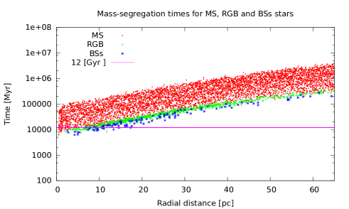
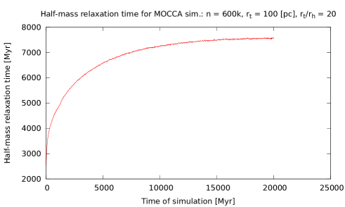
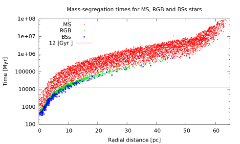
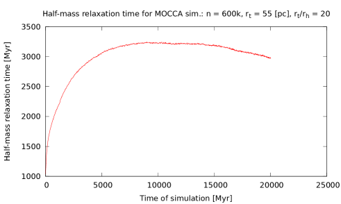
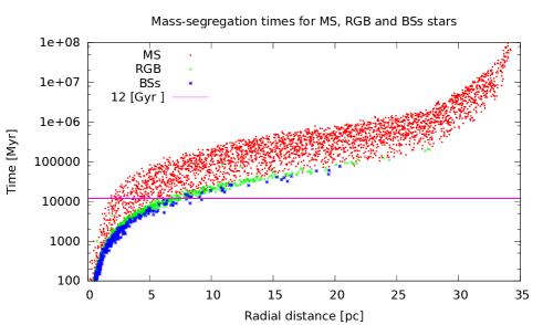
Figure 6: Half-mass relaxation and mass-segregation times for mocca-slow (top row), mocca-medium (middle row) and mocca-fast simulations (bottom row). The first column shows the changes with time of the half-mass relaxation time. The second column contains plots with mass-segregation times for BSs, RGB and MS stars at the time 12 Gyr. The violet line represents the time 12 Gyr itself. For the initial conditions of the models see Tab. 3, and for the discussion of the plots see Sect. 3.2.

For the models with different rates of the dynamical evolution the formation of the signs of bimodal spatial distribution should be different. For the mocca-slow we expected that the bimodality will not be visible for a very long time. Whereas for mocca-fast we expected to observe it earlier and with a larger dip around $r_{avoid}$. Additionally, the drift of $r_{avoid}$ should be also different for the models. For the faster evolving GCs its value in the units of e.g. the core radius should be larger.

Fig. 7 shows the signs of bimodal spatial distribution for mocca-slow (left column), mocca-medium (middle) and mocca-fast simulations (right) for a few selected times for which the bimodal distribution is best visible. The times are specified in the plots’ legends and are given in Myr and in the units of the present $t_{rh}$. The distances on the X axis are given in the units of the core radii ($r_{c}$). Each plot shows three BSs specific frequencies ($R_{BSs}$) calculated for all BSs (red), only the evolutionary BSs (green) and the dynamical ones (blue, except the mocca-slow model for which the number of dynamical BSs is small). Number of BSs in each bin is written on the top of red circles. The errors for the $R_{BSs}$ are calculated as a Poisson error ($R_{BSs}/\sqrt{n_{BSs}}$). Additionally, each plot contains three characteristic radii for a reference: half-light radius ($r_{h~{}obs}$), half-mass radius ($r_{h}$) on the bottom X axis, and the radius of avoidance ($r_{avoid}$) on the top X axis. The radius of avoidance is calculated with Eq. 2 and it is equal to the radius $r$ at which the time of the dynamical friction ($t_{df}$) exceeds the age of the GC. However, a few additional comments concerning the determination of $r_{avoid}$ are needed here. The radius $r_{avoid}$ strongly depends on the local parameters of the GCs. For example, if the local density at some radius r is slightly smaller than the average one, $t_{df}$ can suddenly exceed the age of GC. In order to avoid such randomness, the value of $r_{avoid}$ is actually calculated as the average value from the last 5 $r_{avoid}$ measurements. The average $r_{avoid}$ value is much smoother and less depends on the local GC parameters. Additionally, we decided to use $2\times 100$ neighboring stars around a given test star to calculate the local density and velocity dispersions (see Eq. 2). This number has large impact on the calculated values of $r_{avoid}$ too.

The bins in Fig. 7, and other similar figures presented later, have essentially the same widths for one simulation. Usually the width of bins is 1.0 or 0.5 $r_{c~{}ob}$. However, the number of BSs at larger distances from the center is small, and as a result, errors for later bins are also large. Thus, we decided to join bins into larger ones to increase the amount of BSs per bin. However, this procedure is applied only for bins larger than the calculated $r_{avoid}$. It is consistent with the observational way of presenting the bimodal distribution where bins further from the center are wider too.

The signs of the bimodal distribution in Fig. 7 are best visible for the mocca-fast model. The bimodality for this fast evolving model forms very quick – just after 1 Gyr (0.5 $t_{rh}$) it is already well visible (see the top plot on the right column of Fig. 7). The dip gets bigger with time. After a few Gyr it gets smaller than $R_{BSs}<0.5$ which makes the bimodal distribution more visible. Also the first peak in the center of GC gets bigger with time. It reaches values $R_{BSs}\sim 2.0$ after around 6 Gyr. The time needed to form some signs of the bimodal distribution is comparable to a very low $t_{rh}$ which initially is only around 1.5 Gyr (see Fig. 6).

A similar formation of the bimodal distribution presents mocca-medium model. After 1 Gyr (the top plot in Fig. 7 in the middle column) one can see some sign of a bimodal distribution but the central peak is only $R_{BSs}\sim 1.5$. The bimodality gets more visible with time, and after 9 Gyr (the forth plot in the middle column) is well distinguishable. Here again the formation of the bimodal distribution is comparable to $t_{rh}$. The bimodality starts to be well visible after 4-5 Gyr which corresponds to $t_{rh}~{}\sim~{}6-7~{}Gyr$ at that time (see Fig. 6).

The slowest evolving model, mocca-slow, does not show any signs of bimodal distribution until 6 Gyr (the second plot in Fig. 7 in the left column). Before that time, BSs spatial distributions taking into account errors of $R_{BSs}$ are more or less flat (similarly to the time 0.4 Gyr; the top plot in the left column). The errors for this model are the largest because of the low number of BSs in the bins. The number of EM, and EMT BSs for mocca-slow model is actually the same as for mocca-medium and mocca-fast models (see Fig. 5) but mocca-slow is a much more extended cluster. The BSs for mocca-slow are spread across the whole GC and only in the central regions of GC amount of BSs is around or larger than 10, thus providing a better statistics. The signs of the bimodality are not clearly visible even after 20 Gyr. The overall lack of clear signs of the bimodality is caused by the fact that $t_{rh}$ increases for mocca-slow model from the initial 16 Gyr up to about 36 Gyr after the first few Gyr (see Fig. 6). This is a very slowly evolving GC.

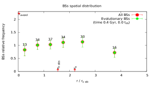
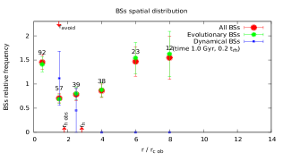
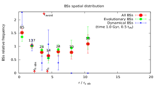
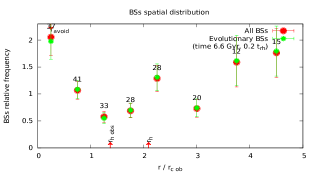
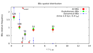
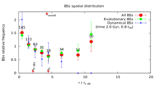
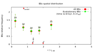
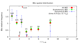
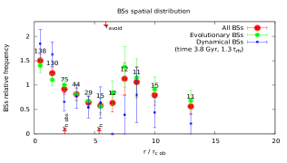
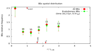
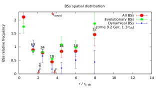
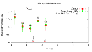
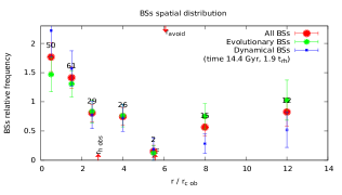
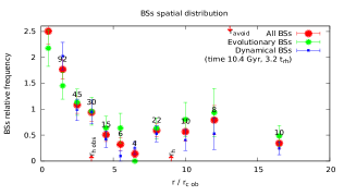
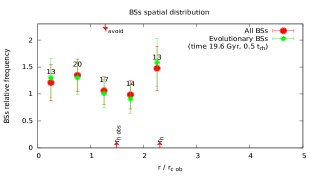
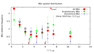
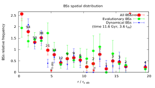
Figure 7: Figure shows the signs of bimodal spatial distribution for mocca-slow (left), mocca-medium (middle) and mocca-fast simulations (right) for a few selected times (in [Myr] and in [$t_{rh}$], see plots’ legends). Each plot contains three characteristic radii for reference: $r_{h~{}obs}$, $r_{h}$ on the bottom X axis, and $r_{avoid}$ on the top X axis. Each plot shows three BSs specific frequencies calculated for all BSs (red), only evolutionary (green) and dynamical ones (blue, except the first column) together with the numbers of all BSs per bins. For detail discussion see Sect. 3.2.

The radius of avoidance goes out of sync after $\sim 2t_{rh}$ (see the middle and right column in Fig. 7). It was rather an unexpected result. Instead, the initial assumptions indicated that the position of $r_{avoid}$ should more or less follow the $r_{min}$, i.e., the radial position at minimum $R_{BSs}$, chosen by eye. Fig. 7 shows the $r_{avoid}$ (on the top X axes) for all three models. For the mocca-fast model $r_{avoid}$ stops to follow the minimum dip already after 6.4 Gyr (2 $t_{rh}$; the forth plot in the right column). The $r_{avoid}$ has to increase with time because it follows the region of GC which has to be affected by the mass segregation. It should constantly increase with time. The same assumptions were made for $r_{min}$, namely that it has to follow more or less the positions of $r_{avoid}$. However, the $r_{min}$ stops to increase with time. After around 10 Gyr $r_{avoid}$ lies even after the second peak (see the second to the last plot in the right column). It corresponds to $>3.0t_{rh}$. For the slower evolving mocca-medium model, $r_{avoid}$ goes out of sync with $r_{min}$ after 16 Gyr (the last plot in the middle column).

As a remark, it is necessary to say that for a few snapshots of mocca-fast model, even after 6 Gyr, the plots with the BSs relative frequency ($R_{BSs}$) show agreement between $r_{avoid}$ and $r_{min}$. But in majority of cases $r_{avoid}$ is clearly out of sync with $r_{min}$. These plots are not shown in the Fig. 7. The randomness of $r_{avoid}$ is discussed in Sect. 3.3.

The bimodal spatial distribution changes to unimodal after several $t_{rh}$. After that time the signs of bimodal distribution appear very rarely. An example of such feature one can see for the mocca-fast model. Thel last plot in Fig. 7 in the right column shows the BSs distribution for the time 11.6 Gyr (3.6 $t_{r}h$). Only the central peak is present, then $R_{BSs}$ drops continuously throughout the whole cluster. In the mocca-fast model after $\sim~{}12$ Gyr BSs are already mass segregated. Almost all BSs at the time of 12 Gyr had already enough time to sink to the center of GC (see mass-segregation time scales in Fig. 6). After 12 Gyr there were a few snapshots for which the bimodal distribution was also visible. However, in majority of cases the distribution was already unimodal. For details on the transientness of the signs of the bimodality see Sect. 3.3. The same feature of transition to unimodal distribution was observed also for other models for which $t_{rh}$ were relatively small (not shown in the paper, though).

Figure 7 shows the BSs specific frequencies for all BSs ($R_{BSs}$, red circles) but also separately for only the evolutionary ($R_{BSs}^{evol}$, green), and the dynamical ones ($R_{BSs}^{dyn}$, blue). There is one feature which is consistent across both mocca-medium and mocca-fast models. For the bins which are before the apparent minimum of the bimodal distributions the values of $R_{BSs}^{evol}$ are consistently below the values of $R_{BSs}$ (red). In turn, the values of $R_{BSs}^{dyn}$ are for the same bins above them. For the bins outside the apparent minimum of the bimodal distributions the situation is reversed. The values of $R_{BSs}^{dyn}$ are consistently below the values of $R_{BSs}$, while the values $R_{BSs}^{evol}$ are consistently above the values of $R_{BSs}$. This situation is a consequence of a several factors. First, the number of dynamical BSs is the highest in the center of a GC because of the higher density there and thus also the higher probabilities for strong dynamical interactions. Second, the dynamical BSs are on average more massive than the evolutionary ones (Hypki & Giersz, 2013, Fig. 6). This causes that the mass segregation times for them are slightly smaller and they can sink faster to the center. Some of the dynamical BSs are ejected due to strong dynamical interactions to larger orbits. Thus, some amount of them can be found far from the center. The last factor is the fact that the evolutionary BSs are being created from unperturbed binaries, so they are created more or less in any part of the system. Thus, the values $R_{BSs}^{evol}$ follow quite closely the values of $R_{BSs}$. The values of $R_{BSs}$ are changed mainly due to the population of dynamical BSs.

3.3 Transientness of the bimodal spatial distribution

The bimodal spatial distribution is very transient. It can be clearly visible in one snapshot and vanish just in the next one (snapshot are written every 200 Myr). Fig. 8 shows a few examples of such transitions between clear signs of the bimodal distribution and the unimodal distribution and vice versa. This change from one state into another can happen actually at any stage of GC evolution, even at later stages when GC is dynamically old. However, after 2-3 $t_{rh}$ the transitions from the unimodal distribution into bimodal are clearly less frequent (see Sect. 3.2).

The transientness of the bimodal distributions is a consequence of the fact that BSs often change their bins. This is also the reason why the values of the BSs relative frequencies vary so much, for the same bins, between two consequent snapshots in time (see Fig. 3). The BSs change their bins due to a combination of a few factors. BSs have small mass-segregation times (see Fig. 6), thus, they can sink to the center faster than RGB or MS stars. Additionally, the orbits of stars around the GC’s center can be elongated (high eccentricity). The time which BSs spend close to their apocenters is larger than in pericenter, but still the high eccentricity of the orbits mean that the radial distances (thus also the bins) for BSs can vary significantly between snapshots. Additionally, the $r_{c}$, which is used to compute BSs relative frequencies, is small in comparison to $r_{h}$. It means that for the bins $\gtrsim r_{h}$ the number of BSs per bin can differ substantially. This is also the reason why it is so important to join bins into larger ones for these bins to see some signs of the bimodal distributions.

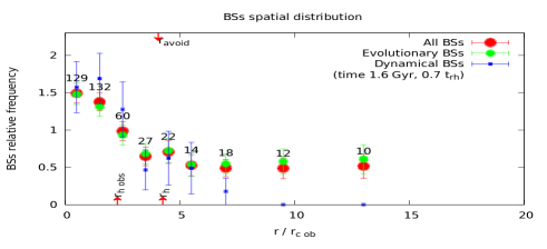
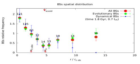
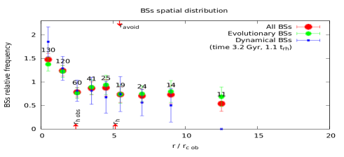
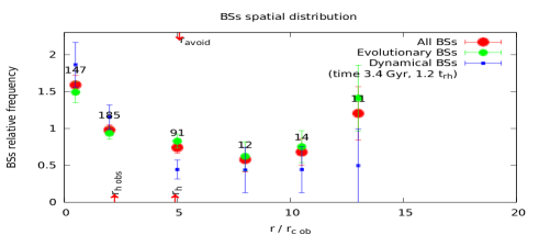
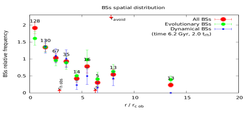
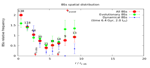
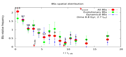
Figure 8: Figure shows a few examples of the transientness of the signs of the bimodal spatial distribution taken only from the mocca-fast simulation. Description of the plots are the same as for Fig. 7. The examples show that between only two snapshots ($\Delta~{}t=200$ Myr, from left to right column) the clear sign of the bimodality can change to unimodal and vice versa. For detailed discussion see Sect. 3.3.

Radius of avoidance ($r_{avoid}$) is rather chaotic and very difficult to compute too. The procedure of its calculation was explained in Sect. 3.2. Fig. 9 shows three examples on how significantly $r_{avoid}$ can change its value between just two consequent snapshots in time ($\Delta~{}t=200$ Myr). Figure shows how unstable the $r_{avoid}$ is for computation of the ,,dynamical clocks” of GCs. The randomness of the $r_{avoid}$ is a result of its large dependence on the local parameters of GCs.

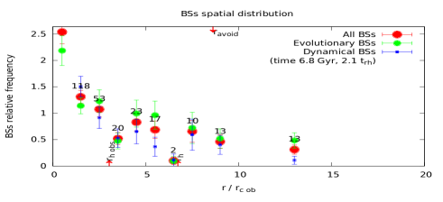
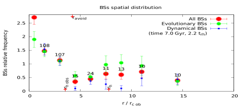
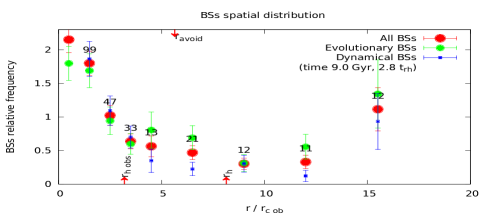
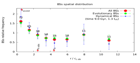
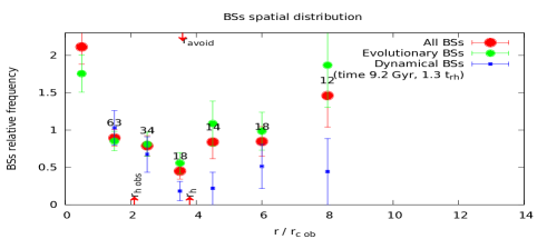
Figure 9: Figure shows three examples on how significantly the radius of avoidance ($r_{avoid}$) can change its value between two consequent snapshots in time ($\Delta~{}t=200$ Myr, from left to right column). The first two rows are taken from mocca-fast and the third one from mocca-medium simulation. The description of the plots is the same as for Fig. 7. For details see Sect. 3.3.

The way of binning has a large impact on the apparent visibility of the bimodal distributions. Too small or too wide bins can obviously hide any signal in any data. However, for the signs of bimodal distribution the procedure of binning histograms seems to be especially important. Fig. 10 shows two examples where just by combining two neighbouring bins into larger ones one can considerably improve the apparent visibility of the bimodal distribution. These examples shows only that the bimodality itself is very noisy. These examples are intended only to make readers sensitive to this problem. By a careful binning one can increase the overall visibility of the bimodal distribution and simultaneously create artificial impression of signals which might not really be present in the data. For example, the widths of bins in Ferraro et al. (2012) are different and look quite random. In this paper the way of binning is kept to be quite simple, and what is most important, consistent for all models (see Sect. 3.2) in order to avoid creation of any artificial signals.

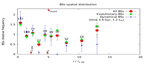
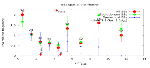
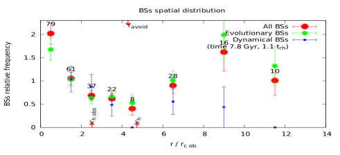
Figure 10: Figure shows two examples on how, only by combining two neighbouring bins into larger ones, one can considerably improve the apparent visibility of the bimodal distribution. These examples are taken from the mocca-fast simulation. The description of the plots is the same as for Fig. 7. For details see Sect. 3.3.

4 Summary and discussion

The goal of this work was to check the evolution of the spatial positions of BSs in GCs. Particularly interesting is the formation of the bimodal distribution of BSs which was already observed in several GCs. This phenomena is also important from the point of view of the dynamical processes which take place in GCs. The formation of the bimodal distribution of BSs is believed to be a result of the mass segregation – the main manifestation of the relaxation processes. In turn, the relaxation describes the age of GCs. Thus, the bimodal distribution might help to determine which GCs are dynamically old and which dynamically young.

The clear sign of the bimodal distribution forms during time comparable with the half-mass relaxation time ($t_{rh}$). Thus, it forms earlier for faster evolving GCs, i.e., these GCs which are denser or have smaller tidal radii (see Sect. 3.2). To check the formation of the bimodal distributions three mocca simulations with different dynamical ages were selected. Only for the slowest evolving model, mocca-slow, the signs of the bimodal distribution were not as clear as for the other models (see Sect. 3.2). For the mocca-slow model the half-mass relaxation time was simply too large and BSs did not have enough time to sink to the center and form a clear central peak.

The bimodal distribution is very transient. It can appear at some point and then vanish after relatively short time ($\sim 200$ Myr, i.e., duration between two subsequent snapshots in time in the mocca simulations). After the next snapshot it may appear again. The mocca-fast model (see Sect. 3.2) is the fastest evolving model from the selected ones. For this model a clear sign of the bimodal distribution forms just after 1 Gyr (see Fig. 7). The half-mass relaxation time changes from $t_{rh}^{T=0}\sim 1.0$ [Gyr] to $t_{rh}^{T=20}\sim 3.0$ [Gyr]. The number of clear signs of the bimodal distribution was observed only in 13 out of 53 snapshots between time 1 Gyr and 11.6 Gyr (interval between the first and the last plot for this model in Fig. 7). It gives 25% chance to see a bimodality for this model. For the model mocca-medium, which evolves a bit slower ($t_{rh}^{T=0}\sim 3$ Gyr, $t_{rh}^{T=20}\sim 7.5$ Gyr), the chance drops to 22% (between 1 and 16.6 Gyr). In other words, it is about 4 times more probable not to see the signs of the bimodal distribution than to actually see it.

The transientness of the signs of bimodal distributions could have important implications for the observations of the real GCs. Fig. 11 shows the GCs with observed bimodal, unimodal and flat distributions marked on the top of all GCs from the Harris catalogue (Harris, 1996). On the X axis there is a half-mass relaxation time ($t_{rh}$) of a GC and on the Y axis – the mass of GC estimated from the M/L relation. Three GCs with flat distributions have large $t_{rh}\gtrsim 10$ Gyr. The bimodal distribution has not been formed for them yet. It is in agreement with the mocca-slow model (see Fig. 7).

The GCs with unimodal and bimodal distributions of BSs intersect each other in Fig. 11. The intersection corresponds to GCs with $t_{rh}\sim 1$ Gyr. The GCs located there should have enough time to form the signs of the bimodal distribution, which they do. However, because of the fact that the bimodality seems to be very transient, the GCs with unimodal distributions occupy the same regions. It is possible that the GCs located there have similar dynamical ages but the signs of the bimodal distributions switches cyclically with the unimodal distributions. This, in turn, implies that the unimodal distributions are not necessarily characteristic for dynamically old GCs which are already well segregated. Because of the transientness, the signs of the bimodal distribution can reappear after a few hundreds of Myr.

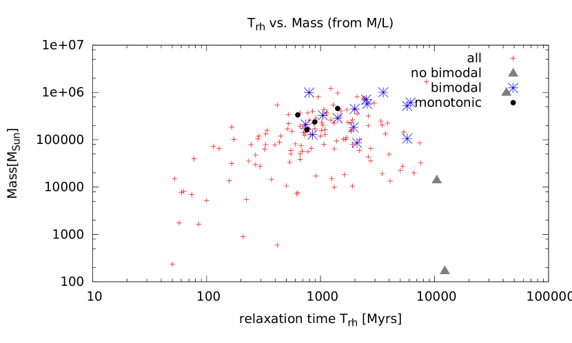
Figure 11: Globular clusters with observed bimodal, unimodal, and flat distributions showed on top of all GCs from the Harris catalogue (Harris, 1996). On the X axis there is the half-mass relaxation time of a GC, while on the Y axis the mass from the M/L relation. The GCs marked with known bimodal distribution are: NGC104, NGC288, NGC5024, NGC5272, NGC5466, NGC5824, NGC5904, NGC6121, NGC6205, NGC6229, NGC6341, NGC6388, NGC6752, NGC6809, NGC7089, with known unimodal distribution: NGC1904, NGC6093, NGC6864, NGC7099 and with known flat distribution: NGC2419, NGC5139, Pal14.

The ,,dynamical clock” proposed by Ferraro et al. (2012) allows to relate the position of the $r_{avoid}$ to the age of GC. However, the simulations from Sect. 3.2 suggest that the ,,dynamical clock” works only for the first $\sim 2t_{rh}$. After that time $r_{avoid}$ goes out of sync with $r_{min}$ (the position of the dip in the bimodal distribution chosen by eye). The position of $r_{avoid}$ keeps increasing its value, while $r_{min}$ stays closer to the center of GC (as the bimodal distribution, see Fig. 7). An example of the real GC which is consistent with this finding is NGC 6388 (see Lanzoni et al. (2007, Fig. 12), Dalessandro et al. (2008b)). The figure presents a clear bimodal distribution of the GC, but the radius $r_{avoid}$ does not correspond to the visible minimum (the place with the lowest number of the relative BSs frequency). The position of $r_{avoid}$ is about $15r_{c}$, whereas the position of the minimum is about 3 times smaller ($5r_{c}$). Dalessandro et al. (2008b) suggests that the dynamical friction, responsible for creating so-called ,,zone of avoidance” (regions around $r_{avoid}$), is not as efficient as previously thought. However, on the basis of this paper, another explanation is argued. The radius $r_{avoid}$ goes out of sync with $r_{min}$ for models if the age of GC exceeds $\sim 2t_{rh}$. If $r_{avoid}$ does not correspond to $r_{min}$, it suggests that NGC 6388 is a dynamically old GC – not dynamically younger as it is stated by Dalessandro et al. (2008b). These authors discuss also the possibility of the existence of IMBH in the center of NGC 6388 but it is not clear how it would affect GC at radii of about $5-15r_{c}$. However, the mocca simulations which do not show agreement between $r_{avoid}$ and $r_{min}$ after $\sim 2t_{rh}$, do not have any IMBHs in their centers. Is is possible that there are GCs with IMBHs in their centers and that for them these two radii would be out of sync too. Nevertheless, the paper shows that there is no need for IMBHs to explain such a feature.

Radius $r_{avoid}$ is found to be very hard to compute. It strongly depends on the local parameters of GCs. Thus, its value can differ significantly between two consequent snapshots in time (200 Myr for all models in Sect. 3). It rises additional difficulties for the ,,dynamical clock” which relates the values of $r_{avoid}$ with the ages of GCs. The mass segregation is in fact the mechanisms which stands behind the formation of the bimodal distributions (see Sect. 3.2). However, the calculations of $r_{avoid}$ in Sect. 3.3 shows and stresses that $r_{avoid}$ is actually a very challenging quantity to compute. Their values should be taken with caution.

It is argued that the ,,dynamical clock” is not as promising tool for dating the dynamical ages of GCs as previously thought. The main challenges constitute the transientness of the signs of the bimodal distribution, the fact that $r_{avoid}$ goes out of sync with the apparent minimum, and the strong dependence of $r_{avoid}$ on the local GC’s parameters.

References

- Aarseth (2003) Aarseth S. J., 2003, Gravitational N-Body Simulations. Cambridge University Press
- Binney & Tremaine (1987) Binney J., Tremaine S., 1987, Galactic dynamics
- Casertano & Hut (1985) Casertano S., Hut P., 1985, ApJ, 298, 80
- Contreras Ramos et al. (2012) Contreras Ramos R., Ferraro F. R., Dalessandro E., Lanzoni B., Rood R. T., 2012, ApJ, 748, 91
- Dalessandro et al. (2008a) Dalessandro E., Lanzoni B., Ferraro F. R., Rood R. T., Milone A., Piotto G., Valenti E., 2008a, ApJ, 677, 1069