Coupled Spin-Light dynamics in Cavity Optomagnonics

Abstract

Experiments during the past two years have shown strong resonant photon-magnon coupling in microwave cavities, while coupling in the optical regime was demonstrated very recently for the first time. Unlike with microwaves, the coupling in optical cavities is parametric, akin to optomechanical systems. This line of research promises to evolve into a new field of optomagnonics, aimed at the coherent manipulation of elementary magnetic excitations by optical means. In this work we derive the microscopic optomagnonic Hamiltonian. In the linear regime the system reduces to the well-known optomechanical case, with remarkably large coupling. Going beyond that, we study the optically induced nonlinear classical dynamics of a macrospin. In the fast cavity regime we obtain an effective equation of motion for the spin and show that the light field induces a dissipative term reminiscent of Gilbert damping. The induced dissipation coefficient however can change sign on the Bloch sphere, giving rise to self-sustained oscillations. When the full dynamics of the system is considered, the system can enter a chaotic regime by successive period doubling of the oscillations.

I Introduction

The ability to manipulate magnetism has played historically an important role in the development of information technologies, using the magnetization of materials to encode information. Today’s research focuses on controlling individual spins and spin currents, as well as spin ensembles, with the aim of incorporating these systems as part of quantum information processing devices. Tserkovnyak et al. (2005); Chumak et al. (2015); Krawczyk and Grundler (2014); Kurizki et al. (2015). In particular the control of elementary excitations of magnetically ordered systems –denominated magnons or spin waves, is highly desirable since their frequency is broadly tunable (ranging from MHz to THz) Stancil and Prabhakar (2009); Chumak et al. (2015) while they can have very long lifetimes, especially for insulating materials like the ferrimagnet yttrium iron garnet (YIG) Serga et al. (2010). The collective character of the magnetic excitations moreover render these robust against local perturbations.

Whereas the good magnetic properties of YIG have been known since the 60s, it is only recently that coupling and controlling spin waves with electromagnetic radiation in solid-state systems has started to be explored. Pump-probe experiments have shown ultrafast magnetization switching with light Stanciu et al. (2007); Kirilyuk et al. (2010); Lambert et al. (2015a), and strong photon-magnon coupling has been demonstrated in microwave cavity experiments Huebl et al. (2013); Zhang et al. (2014); Tabuchi et al. (2014); Goryachev et al. (2014); Bourhill et al. (2015); Haigh et al. (2015a); Bai et al. (2015); Zhang et al. (2015a); Lambert et al. (2015b) –including the photon-mediated coupling between a superconducting qubit and a magnon mode Tabuchi et al. (2015). Going beyond microwaves, this points to the tantalizing possibility of realizing optomagnonics: the coupled dynamics of magnons and photons in the optical regime, which can lead to coherent manipulation of magnons with light. The coupling between magnons and photons in the optical regime differs from that of the microwave regime, where resonant matching of frequencies allows for a linear coupling: one magnon can be converted into a photon, and viceversa Soykal and Flatté (2010); Cao et al. (2015); Zare Rameshti et al. (2015). In the optical case instead, the coupling is a three-particle process. This accounts for the frequency mismatch and is generally called parametric coupling. The mechanism behind the optomagnonic coupling is the Faraday effect, where the angle of polarization of the light changes as it propagates through a magnetic material. Very recent first experiments in this regime show that this is a promising route, by demonstrating coupling between optical modes and magnons, and advances in this field are expected to develop rapidly Zhang et al. (2015b); Haigh et al. (2015b); Zhang et al. (2016); Hisatomi et al. (2016); Osada et al. (2016).

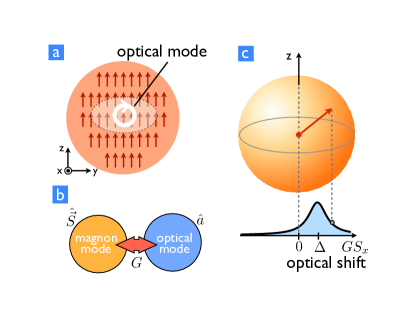
Figure 1: (Color online) Schematic configuration of the model considered. (a) Optomagnonic cavity with homogeneous magnetization along the z-axis and a localized optical mode with circular polarization in the y-z-plane. (b) The homogeneous magnon mode couples to the optical mode with strength $G$. (c) Representation of the magnon mode as a macroscopic spin on the Bloch sphere, whose dynamics is controlled by the coupling to the driven optical mode.

In this work we derive and analyze the basic optomagnonic Hamiltonian that allows for the study of solid-state cavity optomagnonics. The parametric optomagnonic coupling is reminiscent of optomechanical models. In the magnetic case however, the relevant operator that couples to the optical field is the spin, instead of the usual bosonic field representing a mechanical degree of freedom. Whereas at small magnon numbers the spin can be replaced by a harmonic oscillator and the ideas of optomechanics Aspelmeyer et al. (2014) carry over directly, for general trajectories of the spin this is not possible. This gives rise to rich non-linear dynamics which is the focus of the present work. Parametric spin-photon coupling has been studied previously in atomic ensembles Hammerer et al. (2010); Brahms and Stamper-Kurn (2010). In this work we focus on solid-state systems with magnetic order and derive the corresponding optomagnonic Hamiltonian. After obtaining the general Hamiltonian, we consider a simple model which consists of one optical mode coupled to a homogeneous Kittel magnon mode Kittel (1948). We study the classical dynamics of the magnetic degrees of freedom and find magnetization switching, self-sustained oscillations, and chaos, tunable by the light field intensity.

The manuscript is ordered as follows. In Sec. (II) we present the model and the optomagnonic Hamiltonian which is the basis of our work. In Sec. (II.1) we discuss briefly the connection of the optomagnonic Hamiltonian derived in this work and the one used in optomechanic systems. In Sec. (II.2) we derive the optomagnonic Hamiltonian from microscopics, and give an expression for the optomagnonic coupling constant in term of material constants. In Sec. (III) we derive the classical coupled equations of motion of spin and light for a homogeneous magnon mode, in which the spin degrees of freedom can be treated as a macrospin. In Sec. (III.1) we obtain the effective equation of motion for the macrospin in the fast-cavity limit, and show the system presents magnetization switching and self oscillations. We treat the full (beyond the fast-cavity limit) optically induced nonlinear dynamics of the macrospin in Sec. (III.2), and follow the route to chaotic dynamics. In Sec. (IV) we sketch a qualitative phase diagram of the system as a function of coupling and light intensity, and discuss the experimental feasibility of the different regimes. An outlook and conclusions are found in Sec. (V). In the Appendix we give details of some of the calculations in the main text, present more examples of nonlinear dynamics as a function of different tuning parameters, and compare optomagnonic vs. optomechanic attractors.

II Model

Further below, we derive the optomagnonic Hamiltonian which forms the basis of our work:

$$H=-\hbar\Delta\hat{a}^{\dagger}\hat{a}-\hbar\Omega\hat{S}_{z}+\hbar G\hat{S}_{x}\hat{a}^{\dagger}\hat{a}\,,$$ (1)

where $\hat{a}^{\dagger}$ ($\hat{a}$) is the creation (annihilation) operator for a cavity mode photon. We work in a frame rotating at the laser frequency $\omega_{las}$, and $\Delta=\omega_{las}-\omega_{cav}$ is the detuning with respect to the optical cavity frequency $\omega_{cav}$. Eq. (1) assumes a magnetically ordered system with (dimensionless) macrospin ${\bf S}=(S_{x},S_{y},S_{z})$ with magnetization axis along $\mathbf{\hat{z}}$, and a precession frequency $\Omega$ which can be controlled by an external magnetic field . The coupling between the optical field and the spin is given by the last term in Eq. (1), where we assumed (see below) that light couples only to the $x-$ component of the spin as shown in Fig. (1). The coefficient $G$ denotes the parametric optomagnonic coupling. We will derive it in terms of the Faraday rotation, which is a material-dependent constant.

II.1 Relation to optomechanics

Close to the ground state, for deviations such that $\delta S\ll S$ (with $S=|\mathbf{S}|$), we can treat the spin in the usual way as a harmonic oscillator, $\hat{S}_{x}\approx\sqrt{S/2}(\hat{b}+\hat{b}^{\dagger})$, with $\left[\hat{b},\hat{b}^{\dagger}\right]=1$. Then the optomagnonic interaction $\hbar G\hat{S}_{x}\hat{a}^{\dagger}\hat{a}\approx\hbar G\sqrt{S/2}\hat{a}^{\dagger}\hat{a}(\hat{b}+\hat{b}^{\dagger})$ becomes formally equivalent to the well-known optomechanical interaction Aspelmeyer et al. (2014), with bare coupling constant $g_{0}=G\sqrt{S/2}$. All the phenomena of optomechanics apply, including the “optical spring” (here: light-induced changes of the magnon precession frequency) and optomagnonic cooling at a rate $\Gamma_{{\rm{\rm opt}}}$, and the formulas (as reviewed in Ref. Aspelmeyer et al. (2014)) can be taken over directly. All these effects depend on the light-enhanced coupling $g=g_{0}\alpha$, where $\alpha=\sqrt{n_{{\rm phot}}}$ is the cavity light amplitude. For example, in the sideband-resolved regime ($\kappa\ll\Omega$, where $\kappa$ is the optical cavity decay rate) one would have $\Gamma_{{\rm opt}}=4g^{2}/\kappa$. If $g>\kappa$, one enters the strong-coupling regime, where the magnon mode and the optical mode hybridize and where coherent state transfer is possible. A Hamiltonian of the form of Eq. (1) is also encountered for light-matter interaction in atomic ensembles Hammerer et al. (2010), and its explicit connection to optomechanics in this case was discussed previously in Ref. Brahms and Stamper-Kurn (2010). In contrast to such non-interacting spin ensembles, the confined magnon mode assumed here can be frequency-separated from other magnon modes.

II.2 Microscopic magneto-optical coupling $G$

In this section we derive the Hamiltonian presented in Eq. (1) starting from the microscopic magneto-optical effect in Faraday-active materials. The Faraday effect is captured by an effective permittivity tensor that depends on the magnetization $\mathbf{M}$ in the sample. We restrict our analysis to non-dispersive isotropic media and linear response in the magnetization, and relegate magnetic linear birefringence effects which are quadratic in $\mathbf{M}$ (denominated the Cotton-Mouton or Voigt effect) for future work Landau and Lifshitz (1984); Stancil and Prabhakar (2009). In this case, the permittivity tensor acquires an antisymmetric imaginary component and can be written as $\varepsilon_{ij}\left(\mathbf{M}\right)$=$\varepsilon_{0}$$\left(\varepsilon\delta_{ij}-if\sum_{k}\epsilon_{ijk}M_{k}\right)$, where $\varepsilon_{0}$ ($\varepsilon$) is the vacuum (relative) permittivity, $\epsilon_{ijk}$ the Levi-Civita tensor and $f$ a material-dependent constant Landau and Lifshitz (1984) (here and in what follows, Latin indices indicate spatial components). The Faraday rotation per unit length

$$\theta_{F}=\frac{\omega fM_{s}}{2c\sqrt{\varepsilon}}\,,$$ (2)

depends on the frequency $\omega$, the vacuum speed of light $c$, and the saturation magnetization $M_{s}$. The magneto-optical coupling is derived from the time-averaged energy $\bar{U}=\frac{1}{4}\int{\rm d}\mathbf{r}\,\sum_{ij}\,E_{i}^{*}(\mathbf{r},t)\varepsilon_{ij}E_{j}(\mathbf{r},t)$, using the complex representation of the electric field, $\left(\mathbf{E}+\mathbf{E^{*}}\right)/2$. Note that $\bar{U}$ is real since $\varepsilon_{ij}$ is hermitean Landau and Lifshitz (1984); Stancil and Prabhakar (2009). The magneto-optical contribution is

$$\bar{U}_{MO}=-\frac{i}{4}\varepsilon_{0}f\int{\rm d}\mathbf{r}\,\mathbf{M}(\mathbf{r)}\cdot[\mathbf{E^{*}}\left(\mathbf{r}\right)\times\mathbf{E}\left(\mathbf{r}\right)]\,.$$ (3)

This couples the magnetization to the spin angular momentum density of the light field. Quantization of this expression leads to the optomagnonic coupling Hamiltonian. A similar Hamiltonian is obtained in atomic ensemble systems when considering the electric dipolar interaction between the light field and multilevel atoms, where the spin degree of freedom (associated with $\mathbf{M}(\mathbf{r})$ in our case) is represented by the atomic hyperfine structure Hammerer et al. (2010). The exact form of the optomagnonic Hamiltonian will depend on the magnon and optical modes. In photonic crystals, it has been demonstrated that optical modes can be engineered by nanostructure patterning Joannopoulos et al. (2008), and magnonic-crystals design is a matter of intense current research Krawczyk and Grundler (2014). The electric field is easily quantized, $\mathbf{\hat{E}^{(+)}}(\mathbf{r},t)=\sum_{\beta}\mathbf{E}_{\beta}(\mathbf{r})\hat{a}_{\beta}(t)$, where $\mathbf{E}_{\beta}(\mathbf{r})$ indicates the $\beta^{{\rm th}}$ eigenmode of the electric field (eigenmodes are indicated with Greek letters in what follows). The magnetization requires more careful consideration, since $\mathbf{M}(\mathbf{r})$ depends on the local spin operator which, in general, cannot be written as a linear combination of bosonic modes. There are however two simple cases: (i) small deviations of the spins, for which the Holstein-Primakoff representation is linear in the bosonic magnon operators, and (ii) a homogeneous Kittel mode $\mathbf{M}(\mathbf{r})=\mathbf{M}$ with macrospin $\mathbf{S}$. In the following we treat the homogeneous case, to capture nonlinear dynamics. From Eq. (3) we then obtain the coupling Hamiltonian $\hat{H}_{MO}=\hbar\sum_{j\beta\gamma}\hat{S}_{j}G_{\beta\gamma}^{j}\hat{a}_{\beta}^{\dagger}\hat{a}_{\gamma}$ with

$$G_{\beta\gamma}^{j}=-i\frac{\varepsilon_{0}f\,M_{s}}{4\hbar S}\sum_{mn}\epsilon_{jmn}\int{\rm d}\mathbf{r}E_{\beta m}^{*}(\mathbf{r)}E_{\gamma n}(\mathbf{r})\,,$$ (4)

where we replaced $M_{j}/M_{s}=\hat{S}_{j}/S$, with $S$ the extensive total spin (scaling like the mode volume). One can diagonalize the hermitean matrices $G^{j}$, though generically not simultaneously. In the present work, we treat the conceptually simplest case of a strictly diagonal coupling to some optical eigenmodes ($G_{\beta\beta}^{j}\neq 0$ but $G_{\alpha\beta}^{j}=0$). This is precluded only if the optical modes are both time-reversal invariant (${\bf E}_{\beta}$ real-valued) and non-degenerate. In all the other cases, a basis can be found in which this is valid. For example, a strong static Faraday effect will turn optical circular polarization modes into eigenmodes. Alternatively, degeneracy between linearly polarized modes implies we can choose a circular basis.

Consider circular polarization (R/L) in the $y-z$-plane, such that $G^{x}$ is diagonal while $G^{y}=G^{z}=0$. Then we find

$$G_{LL}^{x}=-G_{RR}^{x}=G=\frac{1}{S}\frac{c\,\theta_{F}}{4\sqrt{\varepsilon}}\xi\,,$$ (5)

where we used Eq. (2) to express the coupling via the Faraday rotation $\theta_{F}$, and where $\xi$ is a dimensionless overlap factor that reduces to $1$ if we are dealing with plane waves (see App. A). Thus, we obtain the coupling Hamiltonian $H_{MO}=\hbar G\hat{S}_{x}(\hat{a}_{L}^{\dagger}\hat{a}_{L}-\hat{a}_{R}^{\dagger}\hat{a}_{R})$. This reduces to Eq. (1) if the incoming laser drives only one of the two circular polarizations.

The coupling $G$ gives the magnon precession frequency shift per photon. It decreases for larger magnon mode volume, in contrast to $GS$, which describes the overall optical shift for saturated spin ($S_{x}=S$). For YIG, with $\varepsilon\approx 5$ and $\theta_{F}\approx 200^{{\rm o}}{\rm cm}^{-1}$ Weber (1994); Stancil and Prabhakar (2009), we obtain $GS\approx 10^{10}{\rm Hz}$ (taking $\xi=1$), which can easily become comparable to the precession frequency $\Omega$. The ultimate limit for the magnon mode volume is set by the optical wavelength, $\sim(1\mu m)^{3}$, which yields $S\sim 10^{10}$. Therefore $G\approx 1{\rm Hz}$, whereas the coupling to a single magnon would be remarkably large: $g_{0}=G\sqrt{S/2}\approx 0.1{\rm MHz}$. This provides a strong incentive for designing small magnetic structures, by analogy to the scaling of piezoelectrical resonators Fan et al. (2015). Conversely, for a macroscopic volume of $(1mm)^{3}$, with $S\sim 10^{19}$, this reduces to $G\approx 10^{-9}{\rm Hz}$ and $g_{0}\approx 10{\rm Hz}$.

III Spin dynamics

The coupled Heisenberg equations of motion are obtained from the Hamiltonian in Eq. (1) by using $\left[\hat{a},\hat{a}^{\dagger}\right]=1$, $\left[\hat{S}_{i},\hat{S}_{j}\right]=i\epsilon_{ijk}\hat{S}_{k}$. We next focus on the classical limit, where we replace the operators by their expectation values:

$$\dot{a} = -i\left(GS_{x}-\Delta\right)a-\frac{\kappa}{2}\left(a-\alpha_{{\rm max}}\right)$$

$$\dot{\mathbf{S}} = \left(Ga^{*}a\mathbf{\,e}_{x}-\Omega\,\mathbf{e}_{z}\right)\times\mathbf{S}+\frac{\eta_{{\rm G}}}{S}(\mathbf{\dot{S}}\times\mathbf{S})\,.$$ (6)

Here we introduced the laser amplitude $\alpha_{{\rm max}}$ and the intrinsic spin Gilbert-damping Gilbert (2004), characterized by $\eta_{{\rm G}}$, due to phonons and defects ($\eta_{{\rm G}}\approx 10^{-4}$ for YIG ). After rescaling the fields (see App.. B), we see that the classical dynamics is controlled by only five dimensionless parameters: $\frac{GS}{\Omega},\,\frac{G\alpha_{{\rm max}}^{2}}{\Omega},\,\frac{\Delta}{\Omega},\,\frac{\kappa}{\Omega},\,\eta_{{\rm G}}$. These are independent of $\hbar$ as expected for classical dynamics.

In the following we study the nonlinear classical dynamics of the spin, and in particular we treat cases where the spin can take values on the whole Bloch sphere and therefore differs significantly from a harmonic oscillator, deviating from the optomechanics paradigm valid for $\delta S\ll S$. The optically induced tilt of the spin can be estimated from Eq. (6) as $\delta S/S=G|a|^{2}/\Omega\sim G\alpha_{{\rm max}}^{2}/\Omega=B_{{\rm\alpha_{{\rm max}}}}/\Omega$, where $B_{\alpha_{{\rm max}}}=G\alpha_{{\rm max}}^{2}$ is an optically induced effective magnetic field. We would expect therefore unique optomagnonic behavior (beyond optomechanics) for large enough light intensities, such that $B_{{\rm\alpha_{{\rm max}}}}$ is of the order of or larger than the precession frequency $\Omega$. We will show however that, in the case of blue detuning, even small light intensity can destabilize the original magnetic equilibrium of the uncoupled system, provided the intrinsic Gilbert damping is small.

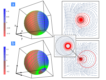
Figure 2: (Color online) Spin dynamics (fast cavity limit) at blue detuning $\Delta=\Omega$ and fixed $GS/\Omega=2$, $\kappa/\Omega=5$, $\eta_{{\rm G}}=0$. The left column depicts the trajectory (green full line) of a spin (initially pointing near the north pole) on the Bloch sphere. The color scale indicates the optical damping $\eta_{{\rm opt}}$. The right column shows a stereographic projection of the spin’s trajectory (red full line). The black dotted line indicates the equator (invariant under the mapping), while the north pole is mapped to infinity. The stream lines of the spin flow are also depicted (blue arrows). (a) Magnetization switching behavior for light intensity $G\alpha_{{\rm max}}^{2}/\Omega=0.36$. (b) Limit cycle attractor for larger light intensity $G\alpha_{{\rm max}}^{2}/\Omega=0.64$.

III.1 Fast cavity regime

As a first step we study a spin which is slow compared to the cavity, where $G\dot{S}_{x}\ll\kappa^{2}$. In that case we can expand the field $a(t)$ in powers of $\dot{S}_{x}$ and obtain an effective equation of motion for the spin by integrating out the light field. We write $a(t)=a_{0}(t)+a_{1}(t)+\ldots$, where the subscript indicates the order in $\dot{S}_{x}$. From the equation for $a(t)$, we find that $a_{0}$ fulfills the instantaneous equilibrium condition

$$a_{0}(t)=\frac{\kappa}{2}\alpha_{{\rm max}}\frac{1}{\frac{\kappa}{2}-i\left(\Delta-GS_{x}(t)\right)}\,,$$ (7)

from which we obtain the correction $a_{1}$:

$$a_{1}(t)=-\frac{1}{\frac{\kappa}{2}-i\left(\Delta-GS_{x}\right)}\frac{\partial a_{0}}{\partial S_{x}}\dot{S}_{x}\,.$$ (8)

To derive the effective equation of motion for the spin, we replace $|a|^{2}\approx|a_{0}|^{2}+a_{1}^{*}a_{0}+a_{0}^{*}a_{1}$ in Eq. (6) which leads to

$$\dot{\mathbf{S}}=\mathbf{B}_{{\rm eff}}\times\mathbf{S}+\frac{\eta_{{\rm opt}}}{S}(\dot{S}_{x}\,\mathbf{e}_{x}\times\mathbf{S})+\frac{\eta_{{\rm G}}}{S}(\mathbf{\dot{S}}\times\mathbf{S})\,.$$ (9)

Here $\mathbf{B}_{{\rm eff}}=-\Omega\mathbf{e}_{z}+\mathbf{B}_{{\rm opt}}$, where $\mathbf{B}_{{\rm opt}}(S_{x})=G|a_{0}|^{2}\,\mathbf{e}_{x}$ acts as an optically induced magnetic field. The second term is reminiscent of Gilbert damping, but with spin-velocity component only along $\mathbf{e}_{x}$. Both the induced field $\mathbf{B}_{{\rm opt}}$ and dissipation coefficient $\eta_{{\rm opt}}$ depend explicitly on the instantaneous value of $S_{x}(t)$:

$$\mathbf{B}_{{\rm opt}} = \frac{G}{[(\frac{\kappa}{2})^{2}+(\Delta-GS_{x})^{2}]}\left(\frac{\kappa}{2}\alpha_{{\rm max}}\right)^{2}\mathbf{e}_{x}$$ (10)

$$\eta_{{\rm opt}} = -2G\kappa S\,|\mathbf{B}_{{\rm opt}}|\,\frac{(\Delta-GS_{x})}{[(\frac{\kappa}{2})^{2}+(\Delta-GS_{x})^{2}]^{2}}\,.$$ (11)

This completes the microscopic derivation of the optical Landau-Lifshitz-Gilbert equation for the spin, an important tool to analyze effective spin dynamics in different contexts Tserkovnyak et al. (2002). We consider the nonlinear adiabatic dynamics of the spin governed by Eq. (9) below. Two distinct solutions can be found: generation of new stable fixed points (magnetic switching) and optomagnonic limit cycles (self oscillations).

Given our Hamiltonian (Eq. (1)), the north pole is stable in the absence of optomagnonic coupling – the selection of this state is ensured by the intrinsic damping $\eta_{{\rm G}}>0$. By driving the system this can change due to the energy pumped to (or absorbed from) the spin, and the new equilibrium is determined by $\mathbf{B}_{{\rm eff}}$ and $\eta_{{\rm opt}}$, when $\eta_{{\rm opt}}$ dominates over $\eta_{{\rm G}}$. Magnetic switching refers to the rotation of the macroscopic magnetization by $\sim\pi$, to a new fixed point near the south pole in our model. This can be obtained for blue detuning $\Delta>0$, in which case $\eta_{{\rm opt}}$ is negative either on the whole Bloch sphere (when $\Delta>GS$) or on a certain region, as shown in Fig. (2)a. Similar results were obtained in the case of spin optodynamics for cold atoms systems Brahms and Stamper-Kurn (2010). The possibility of switching the magnetization direction in a controlled way is of great interest for information processing with magnetic memory devices, in which magnetic domains serve as information bits Stanciu et al. (2007); Kirilyuk et al. (2010); Lambert et al. (2015a). Remarkably, we find that for blue detuning, magnetic switching can be achieved for arbitrary small light intensities in the case of $\eta_{{\rm G}}=0$. This is due to runaway solutions near the north pole for $\Delta>0$, as discussed in detail in App. C. In physical systems, the threshold of light intensity for magnetization switching will be determined by the extrinsic dissipation channels.

For higher intensities of the light field, limit cycle attractors can be found for $|\Delta|<GS$, where the optically induced dissipation $\eta_{{\rm opt}}$ can change sign on the Bloch sphere (Fig. (2)b). The combination of strong nonlinearity and a dissipative term which changes sign, leads the system into self sustained oscillations. The crossover between fixed point solutions and limit cycle attractors is determined by a balance between the detuning and the light intensity, as discussed in App. C. Limit cycle attractors require $B_{{\rm\alpha_{{\rm max}}}}/\Omega>|\Delta|/GS$ (note that from (11) $B_{{\rm opt}}\sim B_{\alpha_{{\rm max}}}$ if $\kappa\gg(\Delta-GS)$ ).

We note that for both examples shown in Fig. (2), for the chosen parameters we have $\eta_{{\rm opt}}\gg\eta_{{\rm G}}$ in the case of YIG, and hence taking $\eta_{{\rm G}}=0$ is a very good approximation. More generally, from Eqs. (10) we estimate $\eta_{opt}\sim GSB_{{\rm opt}}/\kappa^{3}$ and therefore we can safely neglect $\eta_{{\rm G}}$ for $(\alpha_{{}_{{\rm max}}}G)^{2}S\gg\eta_{{\rm G}}\kappa^{3}$. The qualitative results (limit cycle, switching) survive up to $\eta_{opt}\gtrsim\eta_{G}$, although quantitatively modified as $\eta_{{\rm G}}$ is increased: for example, the size of the limit cycle would change, and there would be a threshold intensity for switching.

III.2 Full nonlinear dynamics

The nonlinear system of Eq. (6) presents even richer behavior when we leave the fast cavity regime. For limit cycles near the north pole, when $\delta S\ll S$, the spin is well approximated by a harmonic oscillator, and the dynamics is governed by the attractor diagram established for optomechanics Marquardt et al. (2006). In contrast, larger limit cycles will display novel features unique to optomagnonics, on which we focus here.

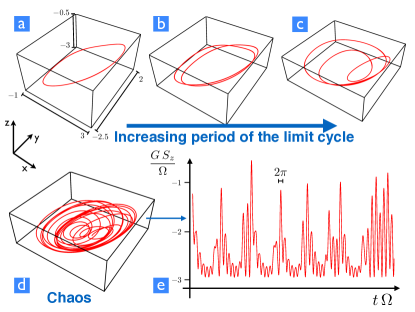
Figure 3: (Color Online) Full non-linear spin dynamics and route to chaos for $GS/\Omega=3$ and $G\alpha_{{\rm max}}^{2}/\Omega=1$ ($\eta_{{\rm G}}=0$). The system is blue detuned by $\Delta=\Omega$ and the dynamics, after a transient, takes place in the southern hemisphere. The solid red curves represent the spin trajectory after the initial transient, on the Bloch sphere for (a) $\kappa/\Omega=3$, (b) $\kappa/\Omega=2$, (c) $\kappa/\Omega=0.9$ , (d) $\kappa/\Omega=0.5$. (f) $S_{z}$ projection as a function of time for the chaotic case $\kappa/\Omega=0.5$.

Beyond the fast cavity limit, we can no longer give analytical expressions for the optically induced magnetic field and dissipation. Moreover, we can not define a coefficient $\eta_{\rm{opt}}$ since an expansion in $\dot{S_{x}}$ is not justified. We therefore resort to numerical analysis of the dynamics. Fig. (3) shows a route to chaos by successive period doubling, upon decreasing the cavity decay $\kappa$. This route can be followed in detail as a function of any selected parameter by plotting the respective bifurcation diagram. This is depicted in Fig. (4). The plot shows the evolution of the attractors of the system as the light intensity is increased. The figure shows the creation and expansion of a limit cycle from a fixed point near the south pole, followed by successive period doubling events and finally entering into a chaotic region. At high intensities, a limit cycle can coexist with a chaotic attractor. For even bigger light intensities, the chaotic attractor disappears and the system precesses around the $\mathbf{\mathbf{e}_{x}}$ axis, as a consequence of the strong optically induced magnetic field. Similar bifurcation diagrams are obtained by varying either $GS/\Omega$ or the detuning $\Delta/\Omega$ (see App. D).

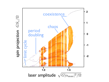
Figure 4: Bifurcation density plot for $GS/\Omega=3$ and $\kappa/\Omega=1$ at $\Delta=\Omega$ ($\eta_{{\rm G}}=0$), as a function of light intensity. We plot the $S_{z}$ values attained at the turning points ($\dot{S}{}_{z}=0$). For other possible choices (eg. $\dot{S}{}_{x}=0$ ) the overall shape of the bifurcation diagram is changed, but the bifurcations and chaotic regimes remain at the same light intensities. For the plot, 30 different random initial conditions were taken.

IV Discussion

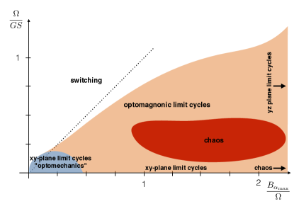
Figure 5: Phase diagram for blue detuning with $\Delta=\Omega$, as a function of the inverse coupling strength $\Omega/GS$ and the optically induced field $B_{\alpha_{{\rm max}}}/\Omega=G\alpha_{{\rm max}}^{2}/\Omega$. Boundaries are qualitative. Switching, in white, refers to a fixed point solution with the spin pointing near the south pole. Limit cycles in the $xy$ plane are shaded in blue, and they follow the optomechanical attractor diagram discussed in Ref. Marquardt et al. (2006). For higher $B_{\alpha_{{\rm max}}}$, chaos can ensue. Orange denotes the parameter space in which limit cycles deviate markedly from optomechanical predictions. These are not in the $xy$ plane and also undergo period doubling leading to chaos. In red is depicted the area where pockets of chaos can be found. For large $B_{\alpha_{{\rm max}}}/\Omega$, the limit cycles are in the $yz$ plane. In the case of red detuning $\Delta=-\Omega$, the phase diagram remains as is, except that instead of switching there is a fixed point near the north pole.

We can now construct a qualitative phase diagram for our system. Specifically, we have explored the qualitative behavior (fixed points, limit cycles, chaos etc.) as a function of optomagnonic coupling and light intensity. These parameters can be conveniently rescaled to make them dimensionless. We chose to consider the ratio of magnon precession frequency to coupling, in the form $\Omega/GS$. Furthermore, we express the light intensity via the maximal optically induced magnetic field $B_{\alpha_{{\rm max}}}=G\alpha_{max}^{2}$. The dimensionless coupling strength, once the material of choice is fixed, can be tuned via an external magnetic field which controls the precession frequency $\Omega$. The light intensity can be controlled by the laser.

We start by considering blue detuning, this is shown in Fig. (5). The “phase diagram” is drawn for $\Delta=\Omega$, and we set $\kappa=\Omega$ and $\eta_{{\rm G}}=0$. We note that some of the transitions are rather crossovers (“optomechanical limit cycles” vs. “optomagnonic limit cycles”). In addition, the other “phase boundaries” are only approximate, obtained from direct inspection of numerical simulations. These are not intended to be exact, and are qualitatively valid for departures of the set parameters, if not too drastic – for example, increasing $\kappa$ will lead eventually to the disappearance of the chaotic region.

As the diagram shows, there is a large range of parameters that lead to magnetic switching, depicted in white. This area is approximately bounded by the condition $B_{\alpha_{{\rm max}}}/\Omega\lesssim\Delta/GS$, which in Fig. (5) corresponds to the diagonal since we took $\Delta=\Omega$. This condition is approximate since it was derived in the fast cavity regime, see App. C. As discussed in Sec. III, magnetic switching should be observable in experiments even for small light intensity in the case of blue detuning, provided that all non-optical dissipation channels are small. The caveat of low intensity is a slow switching time. For $B_{\alpha_{{\rm max}}}/\Omega\gtrsim\Delta/GS$, the system can go into self oscillations and even chaos. For optically induced fields much smaller than the external magnetic field, $B_{\alpha_{{\rm max}}}\ll\Omega$ we expect trajectories of the spin in the $xy$ plane, precessing around the external magnetic field along ${\bf e_{z}}$ and therefore the spin dynamics (after a transient) is effectively two-dimensional. This is depicted by the blue-shaded area in Fig.(5). These limit cycles are governed by the optomechanical attractor diagram presented in Ref. Marquardt et al. (2006), as we show in App. E. There is large parameter region in which the optomagnonic limit cycles deviate from the optomechanical attractors. This is marked by orange in Fig.(5). As the light intensity is increased, for $\Omega/GS\ll 1$ the limit cycles remain approximately confined to the $xy$ plane but exhibit deviations from optomechanics. This approximate confinement of the trajectories to the $xy$ plane at large $B_{\alpha_{{\rm max}}}/\Omega$ ($B_{\alpha_{{\rm max}}}/\Omega\gtrsim 0.5$ for $\Delta=\Omega$) can be understood qualitatively by looking at the expression of the induced magnetic field $B_{{\rm opt}}$ deduced in the fast cavity limit, Eq. (10). Since we consider $\Delta=\Omega$, $\Omega/GS\ll 1$ implies $GS\gg\Delta$. In this limit, $B_{{\rm opt}}/\Omega$ can become very small and the spin precession is around the $\mathbf{e}_{z}$ axis. For moderate $B_{\alpha_{{\rm max}}}/\Omega$ and $\Omega/GS$, the limit cycles are tilted and precessing around an axis determined by the effective magnetic field, a combination of the optical induced field and the external magnetic field. Blue detuning causes these limit cycles to occur in the southern hemisphere. Period doubling leads eventually to chaos. The region where pockets of chaos can be found is represented by red in the phase diagram. For large light intensity, such that $B_{\alpha_{{\rm max}}}\gg\Omega$, the optical field dominates and the effective magnetic field is essentially along the $\mathbf{e_{x}}$ axis. The limit cycle is a precession of the spin around this axis.

According to our results optomagnonic chaos is attained for values of the dimensionless coupling $GS/\Omega\sim 1-10$ and light intensities $G\alpha_{{\rm max}}^{2}/\Omega\sim 0.1-1$. This implies a number of circulating photons similar to the number of locked spins in the material, which scales with the cavity volume. This therefore imposes a condition on the minimum circulating photon density in the cavity. For YIG with characteristic frequencies $\Omega\sim 1-10{\rm GHz}$, the condition on the coupling is easily fulfilled (remember $GS=10{\rm GHz}$ as calculated above). However the condition on the light intensity implies a circulating photon density of $\sim 10^{8}-10^{9}$ photons/${\rm\mu m^{3}}$ which is outside of the current experimental capabilities, limited by the power a typical microcavity can support (around $\sim 10^{5}$ photons/${\rm\mu m^{3}}$). On the other hand, magnetic switching and self-sustained oscillations of the optomechanical type (but taking place in the southern hemisphere) can be attained for low powers, assuming all external dissipation channels are kept small. While self-sustained oscillations and switching can be reached in the fast-cavity regime, more complex nonlinear behavior such as period doubling and chaos requires approaching sideband resolution. For YIG the examples in Figs. 3, 4 correspond to a precession frequency $\Omega\approx 3\cdot 10^{9}{\rm Hz}$ (App. D), whereas $\kappa$ can be estimated to be $\sim 10^{10}{\rm Hz}$, taking into account the light absorption factor for YIG ($\sim 0.3{\rm cm}^{-1}$) Weber (1994).

For red detuning $\Delta<0$, the regions in the phase diagram remain the same, except that instead of magnetic switching, the solutions in this parameter range are fixed points near the north pole. This can be seen by the symmetry of the problem: exchanging $\Delta\rightarrow-\Delta$ together with $\mathbf{e}_{x}\rightarrow-\mathbf{e}_{x}$ and $\mathbf{e}_{z}\rightarrow-\mathbf{e}_{z}$ leaves the problem unchanged. The limit cycles and trajectories follow also this symmetry, and in particular the limit cycles in the $xy$ plane remain invariant.

V Outlook

The observation of the spin dynamics predicted here will be a sensitive probe of the basic cavity optomagnonic model, beyond the linear regime. Our analysis of the optomagnonic nonlinear Gilbert damping could be generalized to more advanced settings, leading to optomagnonic reservoir engineering (e.g. two optical modes connected by a magnon transition). Although the nonlinear dynamics presented here requires light intensities outside of the current experimental capabilities for YIG, it should be kept in mind that our model is the simplest case for which highly non-linear phenomena is present. Increasing the model complexity, for example by allowing for multiple-mode coupling, could result in a decreased light intensity requirement. Materials with a higher Faraday constant would be also beneficial. In this work we focused on the homogeneous Kittel mode. It will be an interesting challenge to study the coupling to magnon modes at finite wavevector, responsible for magnon-induced dissipation and nonlinearities under specific conditions Clogston et al. (1956); Suhl (1957); Gibson and Jeffries (1984). The limit cycle oscillations can be seen as “optomagnonic lasing”, analogous to the functioning principle of a laser where energy is pumped and the system settles in a steady state with a characteristic frequency, and also discussed in the context of mechanics (“cantilaser” Bargatin and Roukes (2003)). These oscillations could serve as a novel source of traveling spin waves in suitable geometries, and the synchronization of such oscillators might be employed to improve their frequency stability. We may see the design of optomagnonic crystals and investigation of optomagnonic polaritons in arrays. In addition, future cavity optomagnonics experiments will allow to address the completely novel regime of cavity-assisted coherent optical manipulation of nonlinear magnetic textures, like domain walls, vortices or skyrmions, or even nonlinear spatiotemporal light-magnon patterns. In the quantum regime, prime future opportunities will be the conversion of magnons to photons or phonons, the entanglement between these subsystems, and their applications to quantum communication and sensitive measurements.

We note that different aspects of optomagnonic systems have been investigated in a related work done simultaneously Liu et al. (2016). Our work was supported by an ERC-StG OPTOMECH and ITN cQOM. H.T. acknowledges support by the Defense Advanced Research Projects Agency (DARPA) Microsystems Technology Office/Mesodynamic Architectures program (N66001-11-1-4114) and an Air Force Office of Scientific Research (AFOSR) Multidisciplinary University Research Initiative grant (FA9550-15-1-0029).

Appendix A Optomagnonic coupling $G$ for plane waves

In this section we calculate explicitly the optomagnonic coupling presented in Eq.. (5) for the case of plane waves mode functions for the electric field. We choose for definiteness the magnetization axis along the $\mathbf{\hat{z}}$ axis, and consider the case $G_{x\beta\gamma}\neq 0$. The Hamiltonian $H_{MO}$ is then diagonal in the the basis of circularly polarized waves, $\mathbf{e}_{R/L}=\frac{1}{\sqrt{2}}\left(\mathbf{e}_{y}\mp i\mathbf{e}_{z}\right)$. The rationale behind choosing the coupling direction perpendicular to the magnetization axis, is to maximize the coupling to the magnon mode, that is to the deviations of the magnetization with respect to the magnetization axis. The relevant spin operator is therefore $\hat{S}_{x}$, which represents the flipping of a spin. In the case of plane waves, we quantize the electric field according to $\mathbf{\hat{E}^{+(-)}}(\mathbf{r},t)=+(-)i\sum_{{}_{j}}\mathbf{e}_{j}\sqrt{\frac{\hbar\omega_{j}}{2\varepsilon_{0}\varepsilon V}}\hat{a}_{j}^{(\dagger)}(t)e^{+(-)i\mathbf{k_{j}\cdot r}}\,,$ where $V$ is the volume of the cavity, $\mathbf{k}_{j}$ the wave vector of mode $j$ and we have identified the positive and negative frequency components of the field as $\mathbf{E}\rightarrow\hat{\mathbf{E}}^{+}$, $\mathbf{E^{*}}\rightarrow\hat{\mathbf{E}}^{-}$. The factor of $\varepsilon_{0}\varepsilon$ in the denominator ensures the normalization $\hbar\omega_{j}=\varepsilon_{0}\varepsilon\langle j|\int d^{3}\mathbf{r}|\mathbf{E}(\mathbf{r})|^{2}|j\rangle-\varepsilon_{0}\varepsilon\langle 0|\int d^{3}\mathbf{r}|\mathbf{E}(\mathbf{r})|^{2}|0\rangle$, which corresponds to the energy of a photon in state $|j\rangle$ above the vacuum $|0\rangle$. For two degenerate (R/L) modes at frequency $\omega$, using Eq. (2) we see that the frequency dependence cancels out and we obtain the simple form for the optomagnonic Hamiltonian $H_{MO}=\hbar G\hat{S}_{x}(\hat{a}_{L}^{\dagger}\hat{a}_{L}-\hat{a}_{R}^{\dagger}\hat{a}_{R})$ with $G=\frac{1}{S}\frac{c\,\theta_{F}}{4\sqrt{\varepsilon}}$. Therefore the overlap factor $\xi=1$ in this case.

Appendix B Rescaled fields and linearized dynamics

To analyze Eq. (6) it is convenient to re-scale the fields such that $a=\alpha_{{\rm max}}a^{\prime}$, ${\bf S}=S{\bf S}^{\prime}$ and measure all times and frequencies in $\Omega$. We obtain the rescaled equations of motion (time-derivatives are now with respect to $t^{\prime}=\Omega t$)

$$\dot{a}^{\prime} = -i(\frac{GS}{\Omega}S_{x}^{\prime}-\frac{\Delta}{\Omega})a^{\prime}-\frac{\kappa}{2\Omega}(a^{\prime}-1)$$ (12)

$$\dot{{\bf S}}^{\prime} = \left(\frac{G\alpha_{{\rm max}}^{2}}{\Omega}|a^{\prime}|^{2}{\bf e}_{x}-{\bf e}_{z}\right)\times{\bf S}^{\prime}+\frac{\eta_{{\rm{G}}}}{S}\left(\dot{\mathbf{S}^{\prime}}\times\mathbf{S}^{\prime}\right)$$ (13)

If we linearize the spin-dynamics (around the north-pole, e.g.), we should recover the optomechanics behavior. In this section we ignore the intrinsic Gilbert damping term. We set approximately ${\bf S}^{\prime}\approx(S^{\prime}_{x},S^{\prime}_{y},1)^{T}$ and from Eq. (12) we obtain

$$\dot{S}_{x}^{\prime} = S^{\prime}_{y}$$ (14)

$$\dot{S}_{y}^{\prime} =- \frac{G\alpha_{{\rm max}}^{2}}{\Omega}|a^{\prime}|^{2}-S^{\prime}_{x}$$ (15)

We can now choose to rescale further, via $S^{\prime}_{x}=\left(\alpha_{{\rm max}}/\sqrt{S}\right)S^{\prime\prime}_{x}$ and likewise for $S_{y}^{\prime}$. We obtain the following spin-linearized equations of motion:

$$\dot{S}_{x}^{\prime\prime} = S^{\prime\prime}_{y}$$ (16)

$$\dot{S}_{y}^{\prime\prime} = -\frac{G\sqrt{S}\alpha_{{\rm max}}}{\Omega}|a^{\prime}|^{2}-S^{\prime\prime}_{x}$$ (17)

$$\dot{a}^{\prime} = -i(\frac{G\sqrt{S}\alpha_{{\rm max}}}{\Omega}S_{x}^{\prime\prime}-\frac{\Delta}{\Omega})a^{\prime}-\frac{\kappa}{2\Omega}(a^{\prime}-1)$$ (18)

This means that the number of dimensionless parameters has been reduced by one, since the two parameters initially involving G, $S$, and $\alpha_{{\rm max}}$ have all been combined into

$$\frac{G\sqrt{S}\alpha_{{\rm max}}}{\Omega}$$ (19)

In other words, for $S^{\prime}_{x,y}=S_{x,y}/S\ll 1$, the dynamics should only depend on this combination, consistent with the optomechanical analogy valid in this regime as discussed in the main text (where we argued based on the Hamiltonian).

Appendix C Switching in the fast cavity limit

From Eq. (9) in the weak dissipation limit ($\eta_{G}\,\ll 1$) we obtain

$$\dot{S}_{x}= \Omega S_{y}$$

$$\dot{S}_{y}= -S_{z}B_{{\rm opt}}-\Omega S_{x}-\frac{\eta_{{\rm opt}}}{S}\dot{S}_{x}S_{z}\,,$$

from where we obtain an equation of motion for $S_{x}$. We are interested in studying the stability of the north pole once the driving is turned on. Hence we set $S_{z}=S$,

$$\ddot{S}_{x}=-\Omega SB_{{\rm opt}}-\Omega^{2}S_{x}-\eta_{{\rm opt}}\Omega\dot{S}_{x}\,,$$

and we consider small deviations $\delta S_{x}$ of $S_{x}$ from the equilibrium position that satisfies $S_{x}^{0}=-SB_{{\rm opt}}/\Omega$, where $B_{{\rm opt}}$ is evaluated at $S_{x}^{0}$. To linear order we obtain

$$\ddot{\delta S}_{x}=-\Omega\left(\Omega+S\frac{\partial B_{{\rm opt}}}{\partial S_{x}}\right)\delta S_{x}+2GS\kappa\Omega B_{{\rm opt}}\frac{(\Delta+GSB_{{\rm opt}}/\Omega)}{\left[\left(\kappa/\Omega\right)^{2}+(\Delta+GSB_{{\rm opt}}/\Omega)^{2}\right]^{2}}\dot{\delta S}_{x}\,.$$

We see that the dissipation coefficient for blue detuning ($\Delta>0$) is always negative, giving rise to runaway solutions. Therefore the solutions near the north pole are always unstable under blue detuning, independent of the light intensity. These trajectories run to a fixed point near the south pole, which accepts stable solutions for $\Delta>0$ (switching) or to a limit cycle. Near the south pole, $S_{z}=-S$, $S_{x}^{0}=SB_{{\rm opt}}/\Omega$ and

$$\ddot{\delta S}_{x}=-\Omega\left(\Omega-S\frac{\partial B_{{\rm opt}}}{\partial S_{x}}\right)\delta S_{x}-2GS\kappa\Omega B_{{\rm opt}}\frac{(\Delta-GSB_{{\rm opt}}/\Omega)}{\left[\left(\kappa/\Omega\right)^{2}+(\Delta-GSB_{{\rm opt}}/\Omega)^{2}\right]^{2}}\dot{\delta S}_{x}\,.$$

Therefore for $\Delta>GSB_{{\rm opt}}/\Omega$ there are stable fixed points, while in the opposite case there are also runaway solutions that are caught in a limit cycle. For red detuning, $\Delta\rightarrow-\Delta$ and the roles of south and north pole are interchanged.

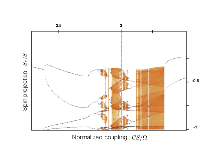
Figure 6: (Color online) Bifurcation density plot for $G\alpha_{{\rm max}}^{2}/\Omega=1$ and $\kappa/\Omega=1$ at $\Delta=\Omega$ ($\eta_{{\rm G}}=0$), as a function of the relative coupling strength $GS/\Omega$. The dotted blue line indicates $GS/\Omega=3$, for comparison with Fig. (4). As in the main text, the points (obtained after the transient) are given by plotting the values of $S_{z}$ attained whenever the trajectory fulfills the turning point condition $\dot{S}{}_{z}=0$, for 20 different random initial conditions.

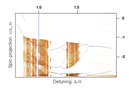
Figure 7: (Color online) Bifurcation density plot for $GS/\Omega=3$, $G\alpha_{{\rm max}}^{2}/\Omega=1$ and $\kappa/\Omega=1$ ($\eta_{{\rm G}}=0$), as a function of the detuning $\Delta/\Omega$. The dotted blue line indicates $\Delta/\Omega=1$, for comparison with Fig. (4).

Appendix D Nonlinear dynamics

In this section we give more details on the full nonlinear dynamics described in the main text. In Figs. 3 and (4) of the main text we chose a relative coupling $GS/\Omega=3$, around which a chaotic attractor is found. With our estimated $GS\approx 10^{10}{\rm Hz}$ for YIG, this implies a precession frequency $\Omega\approx 3\cdot 10^{9}{\rm Hz}$. In Fig. (3) the chaotic regime is reached at $\kappa\approx\Omega/2$ with $G\alpha_{{\rm max}}^{2}/\Omega=1$, which implies $\alpha_{{\rm max}}^{2}\approx S/3$, that is, a number of photons circulating in the (unperturbed) cavity of the order of the number of locked spins and hence scaling with the cavity volume. Bigger values of the cavity decay rate are allowed for attaining chaos at the same frequency, at the expense of more photons in the cavity, as can be deduced from Fig. (4) where we took $\kappa=\Omega$. On the other hand we can think of varying the precession frequency $\Omega$ by an applied external magnetic field and explore the nonlinearities by tuning $GS/\Omega$ in this way (note that $GS$ is a material constant). This is done in Fig. (6). Alternatively, the nonlinear behavior can be controlled by varying the detuning $\Delta$, as shown in Fig. (7).

Appendix E Relation to the optomechanical attractors

In this appendix we show that the optomagnonic system includes the higher order nonlinear attractors found in optomechanics as a subset in parameter space.

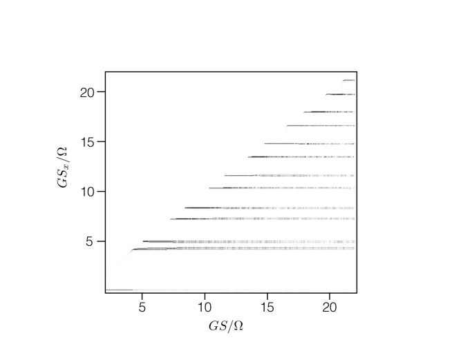
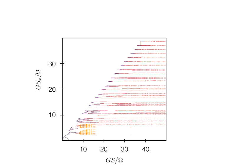
Figure 8: Attractor diagram for $\Delta=1.5\Omega$ and $\kappa/\Omega=1$ with condition $G^{2}S|\alpha_{{\rm max}}|^{2}=n\Omega^{2}$. Top: $n=1$, bottom $n=10$. We plot the $S_{x}$ values attained at the turning points ($\dot{S}_{x}=0$) for $S_{x}>0$. The diagram is symmetric for $S_{x}<0$ as expected for a limit cycle on the Bloch sphere. The diagram at the left coincides to a high degree of approximation with the predictions obtained for optomechanical systems (i.e. replacing the spin by a harmonic oscillator). In contrast, this is no longer the case for the diagram on the right, which involves higher light intensities.

In optomechanics, the high order nonlinear attractors are self sustained oscillations with amplitudes $A$ such that the optomechanical frequency shift $GA$ is a multiple of the mechanical frequency $\Omega$. Translating to our case, this means $G\delta S\sim n\Omega$. Since $\delta S/S\sim G|\alpha_{{\rm max}}|^{2}/\Omega=B_{\alpha_{{\rm max}}}/\Omega$ we obtain the condition

$$\frac{GS}{\Omega}\frac{B_{\alpha_{{\rm max}}}}{\Omega}\sim n\,$$ (20)

for observing these attractors. We can vary $B_{\alpha_{{\rm max}}}$ according to Eq. (20). For $\Omega/GS\ll 1$ we are in the limit of small $B_{\alpha_{{\rm max}}}/\Omega$ and we expect limit cycles precessing along ${\bf e_{z}}$ as discussed in Sec. (IV). In Fig. 8 the attractor diagram obtained by imposing condition (20) is plotted. Since the trajectories are in the $xy$ plane, we plot the inflection point of the coordinate $S_{x}$. We expect $GS_{x}/\Omega$ evaluated at the inflection point, which gives the amplitude of the limit cycle, to coincide with the optomechanic attractors for small $B_{\alpha_{{\rm max}}}/\Omega$ and hence flat lines at the expected amplitudes (as calculated in Ref. Marquardt et al. (2006)) as $GS/\Omega$ increases. Relative evenly spaced limit cycles increasing in number as larger values of $GS/\Omega$ are considered are observed, in agreement with Ref. Marquardt et al. (2006). Remarkable, these limit cycles attractors are found on the whole Bloch sphere, and not only near the north pole where the harmonic approximation is strictly valid. These attractors are reached by allowing initial conditions on the whole Bloch sphere. For $n=1$, (Fig. 8, top), switching is observed up to $GS/\Omega\sim 4$ and then perfect optomechanic behavior. For higher values of $n$, deviations from the optomechanical behavior are observed for small $GS/\Omega$ (implying large $B_{\alpha_{{\rm max}}}/\Omega$ according to Eq. (20)) and large amplitude limit cycles, as compared to the size of the Bloch sphere. An example is shown in Fig. 8, bottom, for $n=10$.

References

- Tserkovnyak et al. (2005) Y. Tserkovnyak, A. Brataas, G. E. W. Bauer, and B. I. Halperin, Reviews of Modern Physics 77, 1375 (2005).
- Chumak et al. (2015) A. V. Chumak, V. I. Vasyuchka, A. A. Serga, and B. Hillebrands, Nature Physics 11, 453 (2015).
- Krawczyk and Grundler (2014) M. Krawczyk and D. Grundler, Journal of physics. Condensed matter : an Institute of Physics journal 26, 123202 (2014).
- Kurizki et al. (2015) G. Kurizki, P. Bertet, Y. Kubo, K. Mølmer, D. Petrosyan, P. Rabl, and J. Schmiedmayer, Proceedings of the National Academy of Sciences 112, 3866 (2015).
- Stancil and Prabhakar (2009) D. D. Stancil and A. Prabhakar, Spin Waves (Springer, 2009).
- Serga et al. (2010) A. A. Serga, A. V. Chumak, and B. Hillebrands, Journal of Physics D: Applied Physics 43, 264002 (2010).
- Stanciu et al. (2007) C. D. Stanciu, F. Hansteen, A. V. Kimel, A. Kirilyuk, A. Tsukamoto, A. Itoh, and T. Rasing, Physical Review Letters 99, 047601 (2007).
- Kirilyuk et al. (2010) A. Kirilyuk, A. V. Kimel, and T. Rasing, Reviews of Modern Physics 82, 2731 (2010).
- Lambert et al. (2015a) C.-H. Lambert, S. Mangin, B. S. D. C. S. Varaprasad, Y. K. Takahashi, M. Hehn, M. Cinchetti, G. Malinowski, K. Hono, Y. Fainman, M. Aeschlimann, and E. E. Fullerton, Science 345, 1337 (2015a).
- Huebl et al. (2013) H. Huebl, C. W. Zollitsch, J. Lotze, F. Hocke, M. Greifenstein, A. Marx, R. Gross, and S. T. B. Goennenwein, Physical Review Letters 111, 127003 (2013).
- Zhang et al. (2014) X. Zhang, C.-l. Zou, L. Jiang, and H. X. Tang, Physical Review Letters 113, 156401 (2014).
- Tabuchi et al. (2014) Y. Tabuchi, S. Ishino, T. Ishikawa, R. Yamazaki, K. Usami, and Y. Nakamura, Physical Review Letters 113, 083603 (2014).
- Goryachev et al. (2014) M. Goryachev, W. G. Farr, D. L. Creedon, Y. Fan, M. Kostylev, and M. E. Tobar, Physical Review Applied 2, 054002 (2014).
- Bourhill et al. (2015) J. Bourhill, N. Kostylev, M. Goryachev, D. Creedon, and M. Tobar, (2015).
- Haigh et al. (2015a) J. A. Haigh, N. J. Lambert, A. C. Doherty, and A. J. Ferguson, Physical Review B 91, 104410 (2015a).
- Bai et al. (2015) L. Bai, M. Harder, Y. P. Chen, X. Fan, J. Q. Xiao, and C.-M. Hu, Physical Review Letters 114, 227201 (2015).
- Zhang et al. (2015a) D. Zhang, X.-M. Wang, T.-F. Li, X.-Q. Luo, W. Wu, F. Nori, and J. You, npj Quantum Information 1, 15014 (2015a).
- Lambert et al. (2015b) N. J. Lambert, J. A. Haigh, and A. J. Ferguson, Journal of Applied Physics 117, 41 (2015b).
- Tabuchi et al. (2015) Y. Tabuchi, S. Ishino, A. Noguchi, T. Ishikawa, R. Yamazaki, K. Usami, and Y. Nakamura, Science 349, 405 (2015), arXiv:1410.3781 .
- Soykal and Flatté (2010) O. Ì. O. Soykal and M. E. Flatté, Physical Review Letters 104, 077202 (2010).
- Cao et al. (2015) Y. Cao, P. Yan, H. Huebl, S. T. B. Goennenwein, and G. E. W. Bauer, Physical Review B 91, 094423 (2015).
- Zare Rameshti et al. (2015) B. Zare Rameshti, Y. Cao, and G. E. W. Bauer, Physical Review B 91, 214430 (2015).
- Zhang et al. (2015b) X. Zhang, N. Zhu, C.-L. Zou, and H. X. Tang, (2015b), arXiv:1510.03545 .
- Haigh et al. (2015b) J. A. Haigh, S. Langenfeld, N. J. Lambert, J. J. Baumberg, A. J. Ramsay, A. Nunnenkamp, and A. J. Ferguson, Physical Review A 92, 063845 (2015b).
- Zhang et al. (2016) X. Zhang, C.-L. Zou, L. Jiang, and H. X. Tang, Science Advances 2, 1501286 (2016).
- Hisatomi et al. (2016) R. Hisatomi, A. Osada, Y. Tabuchi, T. Ishikawa, A. Noguchi, R. Yamazaki, K. Usami, and Y. Nakamura, Physical Review B 93, 174427 (2016).
- Osada et al. (2016) A. Osada, R. Hisatomi, A. Noguchi, Y. Tabuchi, R. Yamazaki, K. Usami, M. Sadgrove, R. Yalla, M. Nomura, and Y. Nakamura, Physical Review Letters 116, 223601 (2016).
- Aspelmeyer et al. (2014) M. Aspelmeyer, T. J. Kippenberg, and F. Marquardt, Reviews of Modern Physics 86, 1391 (2014).
- Hammerer et al. (2010) K. Hammerer, A. S. Soerensen, and E. S. Polzik, Reviews of Modern Physics 82, 1041 (2010).
- Brahms and Stamper-Kurn (2010) N. Brahms and D. M. Stamper-Kurn, Physical Review A 82, 041804 (2010).
- Kittel (1948) C. Kittel, Physical Review 73, 155 (1948).
- Note (1) Note that this frequency however depends on the magnetic field inside the sample, and hence it depends on its geometry and the corresponding demagnetization fields.
- Landau and Lifshitz (1984) L. D. Landau and E. M. Lifshitz, Electrodynamics of continuous media, second edi ed., edited by E. M. Lifshitz and L. P. Pitaevskii (Pergamon Press, 1984).
- Joannopoulos et al. (2008) J. D. Joannopoulos, S. G. Johnson, J. N. Winn, and R. D. Meade, Photonic Crystals, 2nd ed. (Princeton University Press, 2008).
- Weber (1994) M. J. Weber, CRC Handbook of Laser Science and Technology Supplement 2: Optical Materials (CRC Press, 1994).
- Fan et al. (2015) L. Fan, K. Y. Fong, M. Poot, and H. X. Tang, Nature communications 6, 5850 (2015).
- Gilbert (2004) T. Gilbert, IEEE Transactions on Magnetics 40, 3443 (2004).
- Note (2) In the magnetic literature, is denoted as Stancil and Prabhakar (2009).
- Tserkovnyak et al. (2002) Y. Tserkovnyak, A. Brataas, and G. E. W. Bauer, Physical review letters 88, 117601 (2002), 0110247 .
- Marquardt et al. (2006) F. Marquardt, J. G. E. Harris, and S. M. Girvin, Physical Review Letters 96, 103901 (2006).
- Clogston et al. (1956) A. M. Clogston, H. Suhl, L. R. Walker, and P. W. Anderson, J. Phys. Chem. Solids 1, 129 (1956).
- Suhl (1957) H. Suhl, Journal of Physics and Chemistry of Solids 1, 209 (1957).
- Gibson and Jeffries (1984) G. Gibson and C. Jeffries, Physical Review A 29, 811 (1984).
- Bargatin and Roukes (2003) I. Bargatin and M. L. Roukes, Physical review letters 91, 138302 (2003).
- Liu et al. (2016) T. Liu, X. Zhang, H. X. Tang, and M. E. Flatté, (2016), arXiv:1604.07052 .