M(H) dependence and size distribution of SPIONs measured by atomic magnetometry

Abstract

We demonstrate that the quasistatic recording of the magnetic excitation function $M(H)$ of superparamagnetic iron oxide magnetic nanoparticle (SPION) suspensions by an atomic magnetometer allows a precise determination of the sample’s iron mass content $m_{\mathrm{Fe}}$ and the particle size distribution.

1 Introduction

Magnetic nanoparticles (MNP) play a role of increasing importance in biomedical and biochemical applications [1]. The use of MNPs in hyperthermia [2] and as MRI contrast agents [3] is well established, and active studies continue in view of using MNPs for targeted drug delivery [4, 5, 6]. Most MNP applications call for a quantitative characterization and monitoring of the particle distributions both prior to and after their administration into the biological tissue. Two imaging modalities for determining MNP distributions in biological tissues are being actively pursued, viz., magnetorelaxation (MRX) [7] and Magnetic Particle Imaging (MPI) [8].

The superparamagnetic character of the MNPs’ magnetic $M(H)$ response makes magnetic measurements the method of choice for their investigation. High-sensitivity magnetic induction detection plays a key role in view of minimizing the administered MNP dose in biomedical applications. Established MNP characterization/detection methods mainly rely on detecting the oscillating induction $B(t){\propto}M(t)$ induced by a harmonic excitation $H(t)$ with a magnetic pick-up (induction) coil.

Here we describe our successful attempt to replace the pick-up coil by an atomic magnetometer which allows recording quasi-static $B(t)$ variations in frequency ranges that are not accessible to induction coils. Since their introduction in the 1950s [9], atomic magnetometers, also known as optical or optically-pumped magnetometers ($\mathrm{OPM}$) have become important instruments with a broad range of applications [10]. Reports on applications of $\mathrm{OPM}$s for studying MNPs are scarce and have, so far, focused on MRX studies [11, 12, 13].

We have studied the magnetic response $M(H)$ of water-suspended superparamagnetic iron oxide nano-particle samples exposed to time varying excitation fields $H_{\mathrm{drive}}(t)$. We show that an $\mathrm{OPM}$ can be used to record the magnetic induction $B_{\mathrm{\mathrm{NP}}}(t)$ produced by (and proportional to) the time-varying MNP magnetization $M_{\mathrm{\mathrm{NP}}}(t)$, itself proportional to the iron mass content of the sample.

2 Apparatus

The experiments were carried out using the apparatus sketched in Fig. 1 that was mounted in a double aluminum chamber of walk-in size, described by Bison et al. [14]. A major challenge for operating an $\mathrm{OPM}$-based magnetic particle spectrometer lies in the fact that the $\mathrm{OPM}$ has to record fields $B_{\mathrm{\mathrm{NP}}}$ in the pT$\dots$nT range, while being placed as closely as possible to the drive coil producing fields $H_{\mathrm{drive}}$ of several mT/$\mu_{0}$.

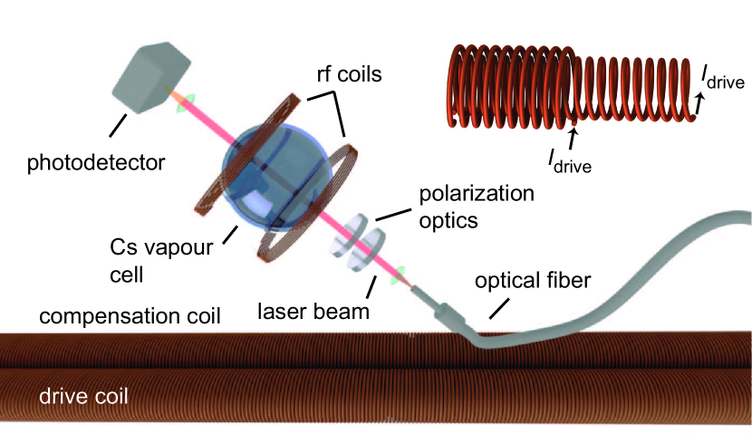
Figure 1: Experimental set-up of the $\mathrm{OPM}$-based MPS. Top right inset: Current flow in the two (opposite handedness) layers in one of the two identical double-layered solenoids. The currents flow in opposite directions in the second double solenoid.

A 70 cm long solenoid with an aspect ratio of 50:1 produces an oscillating drive field $H_{\mathrm{drive}}(t)$ with an amplitude of up to ${\sim}$16 mT${}_{\mathrm{pp}}/\mu_{0}$. The drive solenoid was wound as a double layer of 1.2 mm diameter copper wire on a PVC tube. The two layers have opposite handedness, such that the longitudinal currents originating from the coil’s helicoidal structure (the individual wire loops are not perfectly perpendicular to the solenoid axis) cancel. A second, identical, but oppositely-poled double solenoid, placed next to the drive solenoid, strongly suppresses the stray field originating from the solenoid’s finite aspect ratio. These passive measures reduce the total stray field at the OPM position (at a distance $R\sim$7 cm from the solenoids) by a factor of 10⁶ compared to the field inside of the excitation solenoid.

The $\mathrm{OPM}$ module is similar to the one described by Bison et al. [14], except that the rf field is oriented along the light propagation direction. The sensor uses room-temperature Cs vapour contained in a $\sim$30 mm diameter evacuated and paraffin-coated glass cell. The $\mathrm{OPM}$ is operated as a so-called $M_{x}$ magnetometer, in which a weak magnetic field (rf field) oscillating at frequency $f_{\mathrm{rf}}$ (produced by a pair of small Helmholtz coils) drives the precession of the Cs vapour’s spin polarization around a bias magnetic field $\vec{B}_{0}$ in a resonant, phase-coherent manner. A single circularly-polarized laser beam ($\lambda$=894 nm), locked to the 4-3 hyperfine component of the D₁ transition serves both to create the spin polarization and to detect its precession by monitoring the synchronous modulation of the transmitted laser power. An electronic phase-locked loop (PLL) consisting of a phase detector and a voltage-controlled oscillator ensure that $f_{\mathrm{rf}}$ stays phase-locked to the spin precession frequency

$$f_{\mathrm{prec}}{=}\gamma_{F}\,|\vec{B}_{0}{+}\delta\vec{B}_{\mathrm{\mathrm{NP}}}|\approx\gamma_{F}\left(|\vec{B}_{0}\,|{+}\,\delta\vec{B}_{\mathrm{\mathrm{NP}}}{\cdot}\hat{B}_{0}\right){\equiv}f_{0}+\delta f_{\mathrm{\mathrm{NP}}}\,,$$ (1)

where $\gamma_{F}\approx$ 3.5 Hz/nT, so that $f_{0}{=}$95 kHz in the used bias field $B_{0}$ of 27 $\mu$T. The phase detection and PLL are implemented using a digital lock-in amplifier (Zurich Instruments, model HF2LI, DC—50 MHz) which provides a direct numerical output of the deviations $\delta f_{\mathrm{\mathrm{NP}}}$ that are proportional to the signal of interest $\delta B_{\mathrm{\mathrm{NP}}}$. Although the $M_{x}$ magnetometer is scalar in its nature, it is—to first order—sensitive only to the projection of $\delta\vec{B}_{\mathrm{\mathrm{NP}}}$ onto $\vec{B}_{0}$, since $|\delta\vec{B}_{\mathrm{\mathrm{NP}}}|{\ll}|\vec{B}_{0}|$. It thus acts as a vector component magnetometer like a SQUID.

The bias field $\vec{B}_{0}$ is oriented parallel to the solenoids, in order to maximize the sensitivity to the induction $\delta\vec{B}_{\mathrm{\mathrm{NP}}}$ of interest. The effect of the solenoids’ stray field on $\vec{B}_{0}$ results in a harmonic oscillation of $|\vec{B}_{0}|$ with an amplitude of ${\approx}$3 nT. The magnetometer detects no signal without MNP sample down to its noise floor of $\approx$5 pT$/\sqrt{Hz}$. Under typical experimental conditions the magnetometer can react to magnetic field changes with a bandwidth of $\sim$1 kHz, while keeping the mentioned sensitivity.

3 Measurements and results

We have performed measurements on different MNP samples suspended in aqueous solutions of $\sim$500 $\mu$l contained in sealed glass vessels. The samples can be moved freely through one of the solenoids, and positioned in its center by maximizing the magnetometer signal. Experiments were done by driving the solenoids with a sine-wave-modulated current provided by a high current operational amplifier (Texas Instruments, model OPA541, 5 A max.). We recorded time series (2000 samples per period) of both the magnetometer signal, i.e., its oscillation frequency change $\delta f_{\mathrm{\mathrm{NP}}}$ and the coil current $I_{\mathrm{drive}}$, proportional to the drive field $H_{\mathrm{drive}}(t)$, monitored as the voltage drop over a series resistor. An x–y representation of $\delta f_{\mathrm{\mathrm{NP}}}$ vs. $I_{\mathrm{drive}}$ that is equivalent to $\delta B_{\mathrm{\mathrm{NP}}}$ vs. $H_{\mathrm{drive}}$ after calibration, can then directly be visualized as an oscilloscope trace. Time series of $\delta f_{\mathrm{\mathrm{NP}}}(t)$ and $I_{\mathrm{drive}}(t)$ are stored for further off-line processing. Figure 2 shows a typical example of a recorded $\delta B_{\mathrm{\mathrm{NP}}}(H_{\mathrm{drive}}){\propto}M_{\mathrm{\mathrm{NP}}}(H_{\mathrm{drive}})$ dependence, together with a fitted function and the fit residuals.

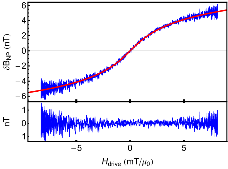
Figure 2: Typical $\delta B_{\mathrm{\mathrm{NP}}}(H_{\mathrm{drive}})$ response of a 0.5 ml Ferrotec EMG${-}707$ sample containing 0.3 mg of iron. The data, representing 50 averaged sinusoidal $H_{\mathrm{drive}}(t)$ cycles (total recording time of $\sim$5 s) are fitted by Eq. 8. The lower graph shows the fit residuals.

Each MNP has a magnetic moment $\mu_{\mathrm{core}}{=}V_{\mathrm{core}}\,M_{S}$, where $V_{\mathrm{core}}{=}4\pi r^{3}/3$ is the particle’s core volume and $M_{s}$ its saturation magnetization. The infinitesimal contribution of particles with radius $r$ to the total magnetic moment is given by

$$\mathrm{d}\mu_{\mathrm{sample}}(H;r)\leavevmode\nobreak\ {=} \mathrm{d}\mu_{\mathrm{core}}(r)\mathcal{L}\left(\frac{H}{H_{k}(r)}\right)$$

$${=} \mathrm{d}N_{\mathrm{\mathrm{NP}}}(r)V_{\mathrm{core}}(r)M_{S}\mathcal{L}\left(\frac{H}{H_{k}(r)}\right)\,,$$ (2)

where the Langevin function $\mathcal{L}(x)=\coth(x)-x^{-1}$ describes the field-dependent degree of magnetization. The saturation field

$$H_{k}(r)=\frac{k_{B}T}{\mu_{0}\mu_{\mathrm{core}}}=\frac{3k_{B}T}{4\pi\mu_{0}r^{3}\,M_{s}}$$ (3)

is a property of the individual particle. The scaling prefactor in Eq. 2, expressed as $\mathrm{d}N_{\mathrm{\mathrm{NP}}}\,V_{\mathrm{core}}{=}\mathrm{d}m_{\mathrm{Fe}}^{\mathrm{tot}}/(\alpha\,\rho_{\mathrm{core}})$, shows that the contribution $\mathrm{d}\mu_{\mathrm{sample}}$ depends in a linear manner on its total iron mass content $\mathrm{d}m_{\mathrm{Fe}}^{\mathrm{tot}}$. In the last expression $\alpha{=}m_{\mathrm{Fe}}/m_{\mathrm{core}}\approx$0.71 is the mass fraction of iron in each nanoparticle’s core, $\rho_{\mathrm{core}}{\equiv}m_{\mathrm{core}}/V_{\mathrm{core}}$ and $m_{\mathrm{core}}$ the core’s density and mass, respectively. With this, Eq. 2 takes the form

$$\mathrm{d}\mu_{\mathrm{sample}}(H;r){=}\frac{\mathrm{d}m_{\mathrm{Fe}}^{\mathrm{tot}}\,M_{S}}{\alpha\,\rho_{\mathrm{core}}}\mathcal{L}\left(\frac{H}{H_{k}(r)}\right)\,.$$ (4)

In practice, the MNP sample shows a size polydispersity that we describe by the lognormal distribution

$$w_{\mathrm{LN}}(r;\mu,k)=\frac{1}{r\sqrt{2\pi k}}\exp\left(-\frac{\ln^{2}(r/\mu)}{2\,k}\right)\,.$$ (5)

The infinitesimal mass of iron in particles of a given size is then expressed as

$$\mathrm{d}m_{\mathrm{Fe}}^{\mathrm{tot}}\leavevmode\nobreak\ =\leavevmode\nobreak\ m_{\mathrm{Fe}}^{\mathrm{tot}}\leavevmode\nobreak\ \frac{r^{3}w_{\mathrm{LN}}(r;\mu,k)}{\mu^{2}e^{\frac{9}{2}k}}\mathrm{d}r=\leavevmode\nobreak\ m_{\mathrm{Fe}}^{\mathrm{tot}}\leavevmode\nobreak\ D(r;\mu,k)\leavevmode\nobreak\ \mathrm{d}r$$ (6)

where $D(r;\mu,k)$ is the mass fraction distribution with mean radius $\overline{r}=\mu\leavevmode\nobreak\ e^{7/2k}$ and standard deviation $\sigma{=}\overline{r}\sqrt{e^{k}-1}$. The distribution $D$ is readily extended to multimodal variants by

$$D_{\mathrm{NP}}^{(n)}(r)=\,\sum_{i=1}^{n}A_{i}D(r;\mu_{i},k_{i})$$ (7)

where $A_{i}$ is the relative mass ratio of the mode $i$ with $\sum_{i=1}^{n}A_{i}{=}1$ and $n$ is the number of modes of the distribution. The magnetic moment of a polydisperse sample is then given by $\mu_{\mathrm{sample}}(H){=}\int_{0}^{\infty}\mathrm{d}\mu_{\mathrm{sample}}(H;r)\,.$ The $\mathrm{OPM}$ detects the far-field magnetic induction

$$\delta B_{\mathrm{\mathrm{NP}}}(H) = \frac{\mu_{0}}{4\pi}\frac{\mu_{\mathrm{sample}}(H)}{R^{3}}=\frac{\mu_{0}}{4\pi R^{3}}\mu_{\mathrm{sample}}^{\mathrm{sat}}\,$$ (8)

$$\times \int\limits_{0}^{\infty}D^{(n)}_{\mathrm{NP}}(r)\mathcal{L}\left(\frac{4\pi\mu_{0}r^{3}M_{S}H}{3k_{B}T}\right)\mathrm{d}r\,,$$

were the saturation ($H{\gg}H_{k}$) value of the sample’s magnetic moment is given by

$$\mu_{\mathrm{sample}}^{\mathrm{sat}}{=}\frac{M_{S}}{\alpha\rho_{\mathrm{core}}}\,m_{\mathrm{Fe}}^{\mathrm{tot}}\,.$$ (9)

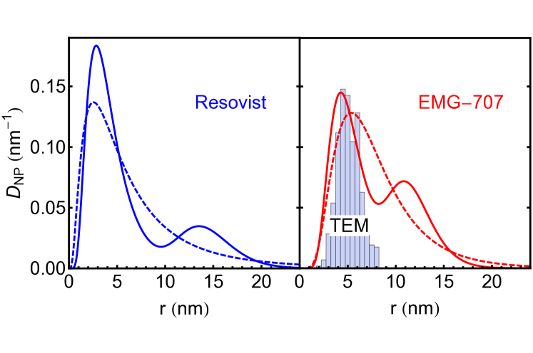
Figure 3: Mono- and bi-modal MNP mass fraction distributions inferred from fits of Eq. 8 to recorded $M(H)$ curves.

We have performed $M(H)$ measurements like the one shown in Fig. 2 on 500 $\mu$l samples in a dilution series of the ferrofluids EMG${-}707$ (from Ferrotec) and Resovist. The experimental parameters ($R$, $T$) and the sample parameters ($\rho_{\mathrm{core}}$, $\alpha$) are known a priori. We use the samples with the highest iron content to obtain the MNP parameters ($M_{S}$ and mass fraction distribution) in the following way: We fit Eq. 8 to the data by fixing the amount of iron as a known parameter derived from manufacturer specifications and the degree of dilution, i.e., $m_{\mathrm{Fe}}^{\mathrm{tot}}{=}m_{\mathrm{Fe}}^{\mathrm{spec}}{=}$4.2 mg for Resovist and $m_{\mathrm{Fe}}^{\mathrm{tot}}{=}m_{\mathrm{Fe}}^{\mathrm{spec}}{=}$10.2 mg for EMG${-}707$, keeping the saturation magnetization $M_{S}$ and the particle mass fraction distribution parameters $\bar{r}_{i}$ and $\sigma_{i}$ as fit parameters. We have performed these calibrations assuming both mono-modal ($n{=}1$) and bi-modal ($n{=}2$) mass fraction distributions. The results are listed in Table 1.

Assuming a monomodal distribution, the fits yield $M_{S}$ and the mass fraction distribution parameters. However, this procedure leads to $M_{S}$ values that are much smaller than the literature/manufacturer values (rows R-1 and E-1 in Table 1). The reason for this discrepancy lies in the fact that because of the modest $H_{\mathrm{drive}}$ field amplitudes used in our experiment we do not strongly saturate the $\mathcal{L}(H_{\mathrm{drive}})$ dependence, so that $M_{S}$ is determined by the linear slope of the $\mathcal{L}(H_{\mathrm{drive}})$ dependence. In the $H_{\mathrm{drive}}{\approx}0$ region, $M_{S}$ is strongly correlated with the mass fraction distribution parameters.

Table 1: Results from fitting magnetization of Resovist (R) and EMG-707 (E) with mono(1)- and bi(2)-modal distributions. Fixed parameters are marked by (f). The distributions of the fits marked with ^∗ are shown in Figure 3.

	$M_{S}$	$\bar{r}_{1}/\sigma_{1}$	$\bar{r}_{2}/\sigma_{2}$	$A_{1}$	FOM
	kA/m	nm	nm		nT
R-1	143	15.4/5.8	–/–	–	0.45
R-1$\ast$	340(f)	7.0/6.8	–/–	–	0.78
R-2$\ast$	340(f)	4.3/2.4	14.5/2.8	0.78	0.43
E-1	279	11.2/3.5	–/–	–	1.01
E-1$\ast$	418(f)	7.9/4.3	–/–	–	1.84
E-2$\ast$	418(f)	5.3/2.1	11.8/2.3	0.64	0.98

In a next step we have fixed (for the fits) the $M_{S}$ values to literature values (340 kA/m [15] for Resovist and 418 kA/m [16] for $\mathrm{EMG}{-}707$), leaving only the mass fraction distribution parameters as fit parameters. The results for monomodal distributions are listed in rows R-1$\ast$ and E-1$\ast$ of Table 1, with corresponding mass fraction distributions shown as dashed lines in Fig. 3. However, the fit qualities of the $M(H)$ dependences obtained with fixed $M_{S}$ values are worse than with free, i.e., fitted $M_{S}$ values, as evidenced by the standard deviations (FOM=figure of merit, listed in Table 1) of the fit residuals.

We next have fitted bi-modal distributions. The bimodal fits yield the $A_{1}$, $\bar{r}_{1}$, $\bar{r}_{2}$, $\sigma_{1}$ and $\sigma_{2}$ values listed in Table 1 as rows R-2 and E-2, respectively. The corresponding distributions are shown as solid lines in Fig. 3. These bimodal fits yield the best FOM of the three outlined procedures. For Resovist the extracted parameters are in agreement with the results of Eberbeck et al. [15]. For $\mathrm{EMG}{-}707$ an agreement of the smaller size mode with the histogram given in Ref. [16] is found.

Freshly produced MNP solutions are basically mono-modal, but, because of cluster formation evolve during aging to a bimodal distribution, as described e.g. in Ref. [15]. The method demonstrated here thus allows a quantitative monitoring of this process.

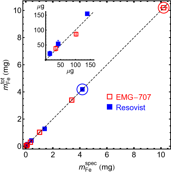
Figure 4: Dependence of the samples’ iron mass $m_{\mathrm{Fe}}^{\mathrm{tot}}$ (inferred from fits by Eq. 8) on the iron mass taken from manufacturer specification and degree of sample dilution, together with slope=1 linear reference line. Circles denote samples used for extraction of MNP parameters. Inset: Data points for small iron contents.

With the size parameter values determined by the calibration procedure we then fit $M(H)$ curves to samples with different dilutions, having $m_{\mathrm{Fe}}^{\mathrm{tot}}$ as only fit parameter. Figure 4 shows the dependence of $m_{\mathrm{Fe}}^{\mathrm{tot}}$ on the mass $m_{\mathrm{Fe}}^{\mathrm{spec}}$ calculated from manufacturer specifications and degree of dilution. We find an excellent agreement, as evidenced by the (non-fitted) slope=1 dashed line in the figure. From the low iron content data points we estimate the current sensitivity to be on the order of $m_{\mathrm{Fe}}^{\mathrm{tot}}\lesssim$7 $\mu$g.

Acknowledgements. Supported by the Swiss National Science Foundation Grant No. 200021_149542.

References

- Huang and Juang [2011] S.-H. Huang and R.-S. Juang. Biochemical and biomedical applications of multifunctional magnetic nanoparticles: a review. J. Nanopart. Res., 13(10):4411–4430, 2011. 10.1007/s11051-011-0551-4.
- Deatsch and Evans [2014] A. E. Deatsch and B. A. Evans. Heating efficiency in magnetic nanoparticle hyperthermia. J. Magn. Magn. Mater., 354:163–172, 2014. 10.1016/j.jmmm.2013.11.006.
- Lee and Hyeon [2012] N. Lee and T. Hyeon. Designed synthesis of uniformly sized iron oxide nanoparticles for efficient magnetic resonance imaging contrast agents. Chem. Soc. Rev., 41(7):2575–2589, 2012. 10.1039/c1cs15248c.
- Arruebo et al. [2007] M. Arruebo, R. Fernándes-Pacheco, M. R. Ibarra, and J. Santamaria. Magnetic nanoparticles for drug delivery. Nanotoday, 2(3):22–32, 2007. 10.1016/S1748-0132(07)70084-1.
- Neuberger et al. [2005] T. Neuberger, B. Schopf, H. Hofmann, M. Hofmann, and B. von Rechenberg. Superparamagnetic nanoparticles for biomedical applications: Possibilities and limitations of a new drug delivery system. J. Magn. Magn. Mater., 293(1, SI):483–496, 2005. 10.1016/j.jmmm.2005.01.064.
- Mahmoudi et al. [2011] M. Mahmoudi, S. Sant, B. Wang, S. Laurent, and T. Sen. Superparamagnetic iron oxide nanoparticles (SPIONs): Development, surface modification and applications in chemotherapy. Adv. Drug Delivery Rev., 63(1-2):24–46, 2011. 10.1016/j.addr.2010.05.006.
- Liebl et al. [2014] M. Liebl, U. Steinhoff, F. Wiekhorst, J. Haueisen, and L. Trahms. Quantitative imaging of magnetic nanoparticles by magnetorelaxometry with multiple excitation coils. Phys. Med. Biol., 59(21):6607, 2014. 10.1088/0031-9155/59/21/6607.
- Panagiotopoulos et al. [2015] N. Panagiotopoulos, R. L. Duschka, M. Ahlborg, G. Bringout, Ch. Debbeler, M. Graeser, Ch. Kaethner, K. Lüdtke-Buzug, H. Medimagh, J. Stelzner, et al. Magnetic particle imaging: current developments and future directions. Int. Journ. Nanomed., 10:3097, 2015. 10.2147/IJN.S70488.
- Dehmelt [1957] H.G. Dehmelt. Modulation of a light beam by precessing absorbing atoms. Phys. Rev., 105(5):1924–1925, 1957. 10.1103/PhysRev.105.1924.
- Budker and Jackson Kimball [2013] D. Budker and D.F. Jackson Kimball. Optical Magnetometry. Cambridge University Press, 2013. 10.1017/CBO9780511846380.
- Maser et al. [2011] D. Maser, S. Pandey, H. Ring, M.P. Ledbetter, S. Knappe, J. Kitching, and D. Budker. Note: Detection of a single cobalt microparticle with a microfabricated atomic magnetometer. Rev. Sci. Instrum., 82:086112, 2011. 10.1063/1.3626505.
- Johnson et al. [2012] C. Johnson, N. L. Adolphi, K. L. Butler, D. M. Lovato, R. Larson, P. D. D. Schwindt, and E. R. Flynn. Magnetic relaxometry with an atomic magnetometer and SQUID sensors on targeted cancer cells. J. Magn. Magn. Mater., 324(17):2613–2619, 2012. 10.1016/j.jmmm.2012.03.015.
- Dolgovskiy et al. [2015] V. Dolgovskiy, V. Lebedev, S. Colombo, A. Weis, B. Michen, L. Ackermann-Hirschi, and A. Petri-Fink. A quantitative study of particle size effects in the magnetorelaxometry of magnetic nanoparticles using atomic magnetometry. J. Magn. Magn. Mater., 379:137–150, 2015. 10.1016/j.jmmm.2014.12.007.
- Bison et al. [2009] G. Bison, N. Castagna, A. Hofer, P. Knowles, J. L. Schenker, M. Kasprzak, H. Saudan, and A. Weis. A room temperature 19-channel magnetic field mapping device for cardiac signals. Appl. Phys. Lett., 95(17):173701, 2009. 10.1063/1.3255041.
- Eberbeck et al. [2013] D. Eberbeck, C. L. Dennis, N. F. Huls, K. L. Krycka, C. Gruttner, and F. Westphal. Multicore magnetic nanoparticles for magnetic particle imaging. IEEE Magn., 49(1):269–274, 2013. 10.1109/TMAG.2012.2226438.
- Gmbh [2006] Ferrotec Gmbh. Application note, 2006. URL www.ferrotec-europe.de/pdf/mnp-kit.app-note4.pdf.