Multiple testing with optimal individual tests
in Gaussian graphical model selection

Abstract

Gaussian Graphical Model selection problem is considered. Concentration graph is identified by multiple decision procedure based on individual tests. Optimal unbiased individual tests are constructed. It is shown that optimal tests are equivalent to sample partial correlation tests. Associated multiple decision procedure is compared with standard procedure.

1 Introduction

Gaussian graphical model (GGM) is a useful and popular tool in biology and genetics Lauritzen (1996), Edwards (2000). This model is based on analysis of conditional independences between random variables which is equivalent to specified zeros among the set of partial correlation coefficients. Some statistical procedures for Gaussian graphical model selection are proposed and investigated in Dempster (1972), Edwards (2000). Statistical procedures in Edwards (2000) does not control family wise error rate (FWER). To overcome this issue multiple single-step and stepwise statistical procedures were recently introduced (see Drton and Perlman (2004), Drton and Perlman (2007), Drton and Perlman (2008) and references therein). Majority of multiple testing procedures are based on statistics for individual hypotheses testing. Usually, sample partial correlations are used as natural test statistics for testing individual hypotheses. However, as far as we know, properties of optimality of these tests were not well investigated so far. In the present paper we construct an optimal unbiased test of the Neyman structure for testing individual hypotheses in GGM selection and prove that these tests are equivalent to sample partial correlation tests. Numerical experiments are conducted to compare the multiple testing procedure with optimal individual tests with standard concentration graph identification procedure based on Fisher z-transform of sample partial correlations.

The paper is organized as follows. Section 2 contains basic definition and problem statement. In the Section 3 a general description of the tests of the Neyman structure is given. In the Section 4 optimal tests for testing individual hypotheses are constructed. In the Section 5 the main result of optimality of the sample partial correlation test is proved. Multiple testing procedure with optimal individual tests is presented in 6 and it is compared with standard Bonferroni procedure. Concluding remarks are given in the Section 7.

2 Basic notations and problem statement

Let random vector $X=(X_{1},X_{2},\ldots,X_{N})$ has a multivariate Gaussian distribution $N(\mu,\Lambda)$, where $\mu=(\mu_{1},\mu_{2},\ldots,\mu_{N})$ is the vector of means and $\Lambda=(\sigma_{i,j})$ is the covariance matrix, $\sigma_{i,j}=\mbox{cov}(X_{i},X_{j})$, $i,j=1,2,\ldots,N$. Denote by $\rho_{i,j}$ Pearson correlation between random variables $X_{i}$, $X_{j}$, $\rho_{i,j}=\sigma_{i,j}/\sqrt{\sigma_{i,i}\sigma_{j,j}}$. Let $x(t)$, $t=1,2,\ldots,n$ be a sample of the size $n$ from distribution $X$. Let

$$s_{i,j}=\frac{1}{n}\Sigma_{t=1}^{n}(x_{i}(t)-\overline{x_{i}})(x_{j}(t)-\overline{x_{j}}),\ \ \overline{x_{i}}=(1/n)\sum_{t=1}^{n}x_{i}(t)$$

be the sample covariance between $X_{i}$, $X_{j}$. Let $S=(s_{i,j})$ be the matrix of sample covariances. Denote by $r_{i,j}$ the sample Pearson correlation between random variables $X_{i}$, $X_{j}$, $r_{i,j}=s_{i,j}/\sqrt{s_{i,i}s_{j,j}}$. It is known Anderson (2003), that the statistics $\overline{x}=(\overline{x_{1}},\overline{x_{2}},...,\overline{x_{N}})$ and $S=(s_{i,j})$ are sufficient for multivariate Gaussian distribution. The inverse matrix for $\Lambda$, $\Lambda^{-1}=(\sigma^{i,j})$ is known as concentration or precision matrix for the distribution $X$.

Consider the set $\cal{G}$ of all $N\times N$ symmetric matrices $G=(g_{i,j})$ with $g_{i,j}\in\{0,1\}$, $i,j=1,2,\ldots,N$, $g_{i,i}=0$, $i=1,2,\ldots,N$. Matrices $G\in\cal{G}$ represent adjacency matrices of all simple undirected graphs with $N$ vertices. Total number of matrices in $\cal{G}$ equals to $L=2^{M}$ with $M=N(N-1)/2$. The problem of Gaussian graphical model selection can be formulated now as a multiple decision problem of selecting one from a set of $L$ hypotheses:

$$H_{G}:\sigma^{i,j}=0,\mbox{ if }g_{i,j}=0,\ \ \sigma^{i,j}\neq 0,\mbox{ if }g_{i,j}=1;\ \ i\neq j$$ (1)

For the multiple decision problem (1) we introduce the following set of individual hypotheses:

$$h_{i,j}:\sigma^{i,j}=0\mbox{ vs }\ k_{i,j}:\sigma^{i,j}\neq 0,\\ \ i,\ j=1,2,\ldots,N,\ i\neq j.$$ (2)

In this paper we consider individual tests for (2) of the following form

$$\varphi_{i,j}(x)=\left\{\begin{array}[]{lll}0,&\mbox{if}&c^{1}_{i,j}<T_{i,j}<c^{2}_{i,j}\\ 1,&\mbox{otherwise}&\end{array}\right.$$ (3)

where $T_{i,j}(x)$, are the tests statistics. There are many multiple testing procedures based on simultaneous use of individual tests statistics: Bonferroni, Holm, Hochberg, Simes, T-max procedures and others. In this paper we concentrate on Bonferroni multiple testing procedures with optimal individual tests.

3 Tests of the Neyman structure

To construct optimal individual tests for the problem (2) we use a tests of the Neyman structure Lehmann and Romano (2005), Koldanov and Koldanov (2014). Let $f(x;\theta)$ be the density of the exponential family:

$$f(x;\theta)=c(\theta)exp(\sum_{j=1}^{M}\theta_{j}T_{j}(x))m(x)$$ (4)

where $c(\theta)$ is a function defined in the parameters space, $m(x)$, $T_{j}(x)$ are functions defined in the sample space $R^{N\times n}$, and $T_{j}(X)$ are the sufficient statistics for $\theta_{j},j=1,\ldots,M$.

Suppose that individual hypotheses have the form:

$$h_{j}:\theta_{j}=\theta^{0}_{j}\mbox{ vs }k_{j}:\theta_{j}\neq\theta^{0}_{j},\ \ j=1,2,\ldots,M$$ (5)

where $\theta^{0}_{j}$ are fixed.

The optimal unbiased tests for individual hypotheses (5) are (see Lehmann and Romano (2005) ch. 4, theorem 4.4.1):

$$\varphi_{j}=\left\{\begin{array}[]{lc}0,&\mbox{if}\ \ c^{1}_{j}(t_{1},\ldots,t_{j-1},t_{j+1},\ldots,t_{M})<t_{j}<c^{2}_{j}(t_{1},\ldots,t_{j-1},t_{j+1},\ldots,t_{M})\\ 1,&\mbox{ otherwise }\end{array}\right.$$ (6)

where $t_{i}=T_{i}(x),i=1,\ldots,M$ and constants $c^{1}_{j}$, $c^{2}_{j}$ are defined from the equations

$$\int_{c^{1}_{j}}^{c^{2}_{j}}f(t_{j},\theta^{0}_{j}|T_{i}=t_{i},i=1,\ldots,M;i\neq j)dt_{j}=1-\alpha_{j}$$ (7)

and

$$\begin{array}[]{l}\int_{-\infty}^{c^{1}_{j}}t_{j}f(t_{j},\theta^{0}_{j}|T_{i}=t_{i},i=1,\ldots,M;i\neq j)dt_{j}+\\ +\int_{c^{2}_{j}}^{+\infty}t_{j}f(t_{j},\theta^{0}_{j}|T_{i}=t_{i},i=1,\ldots,M;i\neq j)dt_{j}=\\ =\alpha_{j}\int_{-\infty}^{+\infty}t_{j}f(t_{j},\theta^{0}_{j}|T_{i}=t_{i},i=1,\ldots,M;i\neq j)dt_{j}\end{array}$$ (8)

where $f(t_{j},\theta^{0}_{j}|T_{i}=t_{i},i=1,\ldots,M;i\neq j)$ is the density of conditional distribution of statistics $T_{j}$ and $\alpha_{j}$ is the significance level of the test.

4 Optimal individual tests

Now we construct the optimal test in the class of unbiased tests for individual hypothesis (2). This construction is based on the tests of the Neyman structure. Joint distribution of sufficient statistics $s_{k,l}$, $k,l=1,2,\ldots,N$ is given by Wishart density function Anderson (2003):

$$f(\{s_{k,l}\})=\displaystyle\frac{[\det(\sigma^{k,l})]^{n/2}\times[\det(s_{k,l})]^{(n-N-2)/2}\times\exp[-(1/2)\sum_{k}\sum_{l}s_{k,l}\sigma^{k,l}]}{2^{(Nn/2)}\times\pi^{N(N-1)/4}\times\Gamma(n/2)\Gamma((n-1)/2)\cdots\Gamma((n-N+1)/2)}$$

if the matrix $(s_{k,l})$ is positive definite, and $f(\{s_{k,l}\})=0$ otherwise. For a fixed $(i,j)$ one has:

$$f(\{s_{k,l}\})=\displaystyle C(\{\sigma^{k,l}\})\exp[-\sigma^{i,j}s_{i,j}-\frac{1}{2}\sum_{(k,l)\neq(i,j);(k,l)\neq(j,i)}s_{k,l}\sigma^{k,l}]m(\{s_{k,l}\})$$

where

$$C(\{\sigma^{k,l}\})=c_{1}^{-1}[\det(\sigma^{k,l})]^{n/2}$$

$$c_{1}=2^{(Nn/2)}\times\pi^{N(N-1)/4}\times\Gamma(n/2)\Gamma((n-1)/2)\cdots\Gamma((n-N+1)/2)$$

$$m(\{s_{k,l}\})=[\det(s_{k,l})]^{(n-N-2)/2}$$

According to (6) the optimal test in the class of unbiased tests for the individual hypothesis (2) has the form:

$$\varphi_{i,j}(\{s_{kl}\})=\left\{\begin{array}[]{rl}\ 0,&\mbox{}\>if\>c_{i,j}^{1}(\{s_{k,l}\})<s_{ij}<c_{i,j}^{2}(\{s_{k,l}\}),\ (k,l)\neq(i,j)\\ \ 1,&\mbox{}\>if\>s_{ij}\leq c_{i,j}^{1}(\{s_{kl}\})\mbox{ or }s_{i,j}\geq c_{i,j}^{2}(\{s_{k,l}\}),\ (k,l)\neq(i,j)\end{array}\right.$$ (9)

where according to (7),(8) the critical values $c_{i,j}$ are defined from the equations

$$\frac{\int_{I\cap[c_{i,j}^{1};c_{i,j}^{2}]}[\det(s_{k,l})]^{(n-N-2)/2}ds_{i,j}}{\int_{I}[\det(s_{k,l})]^{(n-N-2)/2}ds_{i,j}}=1-\alpha_{i,j}$$ (10)

$$\begin{array}[]{l}\displaystyle\int_{I\cap[-\infty;c_{i,j}^{1}]}s_{i,j}[\det(s_{k,l})]^{(n-N-2)/2}ds_{i,j}+\\ +\displaystyle\int_{I\cap[c_{i,j}^{2};+\infty]}s_{i,j}[\det(s_{k,l})]^{(n-N-2)/2}ds_{i,j}=\\ =\alpha_{i,j}\int_{I}s_{i,j}[\det(s_{k,l})]^{(n-N-2)/2}ds_{i,j}\end{array}$$ (11)

where $I$ is the interval of values of $s_{i,j}$ such that the matrix $(s_{k,l})$ is positive definite and $\alpha_{i,j}$ is the significance level of the tests.

Consider $\det(s_{k,l})$ as a function of the variable $s_{i,j}$. This determinant is a quadratic polynomial of $s_{i,j}$:

$$\det(s_{k,l})=-as_{i,j}^{2}+bs_{i,j}+c$$ (12)

Let $K=(n-N-2)/2$. Denote by $x_{1},x_{2}$ the roots of the equation $-ax^{2}+bx+c=0$. One has with the change of variable $x=x_{1}+(x_{2}-x_{1})u$:

$$\int_{f}^{d}(ax^{2}-bx-c)^{K}dx=\displaystyle(-1)^{K}a^{K}(x_{2}-x_{1})^{2K+1}\int_{\frac{f-x_{1}}{x_{2}-x_{1}}}^{\frac{d-x_{1}}{x_{2}-x_{1}}}u^{K}(1-u)^{K}du$$

Therefore the equation (10) takes the form:

$$\int_{\frac{c^{1}-x_{1}}{x_{2}-x_{1}}}^{\frac{c^{1}-x_{1}}{x_{2}-x_{1}}}u^{K}(1-u)^{K}du=(1-\alpha)\int_{0}^{1}u^{K}(1-u)^{K}du$$ (13)

or

$$\frac{\Gamma(2K+2)}{\Gamma(K+1)\Gamma(K+1)}\int_{\frac{c^{1}-x_{1}}{x_{2}-x_{1}}}^{\frac{c^{1}-x_{1}}{x_{2}-x_{1}}}u^{K}(1-u)^{K}du=(1-\alpha)$$ (14)

It means that conditional distribution of $s_{i,j}$ when all other $s_{k,l}$ are fixed is the beta distribution $Be(K+1,K+1)$.

Beta distribution $Be(K+1,K+1)$ is symmetric with respect to the point $\frac{1}{2}$. Therefore the significance level condition (10) and unbiasedness condition (11) are satisfied if and only if:

$$\frac{c^{2}-x_{1}}{x_{2}-x_{1}}=1-\frac{c^{1}-x_{1}}{x_{2}-x_{1}}$$

Let $q$ be the $\frac{\alpha}{2}(\alpha<\frac{1}{2})$-quantile of beta distribution $Be(K+1,K+1)$, i.e. $F_{Be}(q)=\frac{\alpha}{2}$. Then thresholds $c^{1}$, $c^{2}$ are defined by:

$$\begin{array}[]{c}c^{1}=x_{1}+(x_{2}-x_{1})q\\ c^{2}=x_{2}-(x_{2}-x_{1})q\end{array}$$ (15)

Finally, the test of the Neyman structure accepts the hypothesis $\sigma^{i,j}=0$ vs alternative $\sigma^{i,j}\neq 0$ iff:

$$c^{1}_{i,j}<s_{i,j}<c^{2}_{i,j}$$ (16)

where

$$\begin{array}[]{l}c^{1}_{i,j}=x_{1}(i,j)+(x_{2}(i,j)-x_{1}(i,j))q(\alpha_{i,j})\\ c^{1}_{i,j}=x_{2}(i,j)-(x_{2}(i,j)-x_{1}(i,j))q(\alpha_{i,j})\end{array}$$

and $F_{Be}(q(\alpha_{i,j}))=\alpha_{i,j}/2$, $x_{1},x_{2}$ are defined from the equation $ax^{2}-bx-c=0$ with $a,b,c$ defined in (12). The test (16) can be written in the following form

$$\varphi_{i,j}=\left\{\ \begin{array}[]{ll}0,&\displaystyle 2q-1<\frac{as_{i,j}-\frac{b}{2}}{\sqrt{\frac{b^{2}}{4}+ac}}<1-2q\\ 1,&\mbox{otherwise}\end{array}\right.$$ (17)

where $a=a_{i,j},b=b_{i,j},c=c_{i,j}$ are defined in (12).

5 Optimality of the sample partial correlation tests

It is known Lauritzen (1996) that hypothesis $\sigma^{i,j}=0$ is equivalent to the hypothesis $\rho^{i,j}=0$, where $\rho^{i,j}$ is the saturated partial correlation between $X_{i}$ and $X_{j}$:

$$\rho^{i,j}=\frac{-\Lambda_{i,j}}{\sqrt{\Lambda_{i,i}\Lambda_{j,j}}}$$

where for a given matrix $A=(a_{k,l})$ we denote by $A_{i,j}$ the cofactor of the element $a_{i,j}$. Denote by $r^{i,j}$ a sample partial correlation

$$r^{i,j}=\frac{-S_{i,j}}{\sqrt{S_{i,i}S_{j,j}}}$$

where $S_{i,j}$ is the cofactor of the element $s_{i,j}$ in the matrix of sample covariances $S$.

Test for testing hypothesis $\rho^{i,j}=0$ has the form Anderson (2003):

$$\varphi_{i,j}=\left\{\ \begin{array}[]{ll}0,&|r^{i,j}|\leq c_{i,j}\\ 1,&|r^{i,j}|>c_{i,j}\end{array}\right.$$ (18)

where $c_{i,j}$ is $(1-\alpha_{i,j}/2)$-quantile of the distribution with the following density function

$$f(x)=\displaystyle\frac{1}{\sqrt{\pi}}\frac{\Gamma(n-N+1)/2)}{\Gamma((n-N)/2)}(1-x^{2})^{(n-N-2)/2},\ \ \ -1\leq x\leq 1$$

In practical applications the following Fisher transformation is used:

$$z_{i,j}=\frac{\sqrt{n}}{2}\ln\left(\frac{1+r^{i,j}}{1-r^{i,j}}\right)$$

For the case $\rho^{i,j}=0$ statistic $z_{i,j}$ asymptotically has standard Gaussian distribution. That is why the following test is largely used Anderson (2003), Drton and Perlman (2007):

$$\varphi_{i,j}=\left\{\ \begin{array}[]{ll}0,&|z_{i,j}|\leq c_{i,j}\\ 1,&|z_{i,j}|>c_{i,j}\end{array}\right.$$ (19)

where the constant $c_{i,j}$ is $(1-\alpha_{i,j}/2)$-quantile of standard Gaussian distribution.

In this section we prove that optimal unbiased test (17) is equivalent to the test (18).

Theorem: Sample partial correlation test (18) is optimal in the class of unbiased tests for testing hypothesis $\rho^{i,j}=0$ vs $\rho^{i,j}\neq 0$.

Proof: it is sufficient to prove that

$$\frac{S_{i,j}}{\sqrt{S_{i,i}S_{j,j}}}=\frac{as_{i,j}-\frac{b}{2}}{\sqrt{\frac{b^{2}}{4}+ac}}$$ (20)

To prove this equation we introduce some notations. Let $A=(a_{k,l})$ be an $(N\times N)$ symmetric matrix. Fix $i<j$, $i,j=1,2,\ldots,N$. Denote by $A(x)$ the matrix obtained from $A$ by replacing the elements $a_{i,j}$ and $a_{j,i}$ by $x$. Denote by $A_{i,j}(x)$ the cofactor of the element $(i,j)$ in the matrix $A(x)$. Then the following statement is true

Lemma: One has $[\mbox{det}A(x)]^{\prime}=-2A_{i,j}(x)$.

Proof of the Lemma: one has from the general Laplace decomposition of $\det A(x)$ by two rows $i$ and $j$:

$$\det(A(x))=\det\left(\begin{array}[]{ll}a_{i,i}&x\\ x&a_{j,j}\\ \end{array}\right)A_{\{i,j\},\{i,j\}}+\sum_{k<j,k\neq i}\det\left(\begin{array}[]{ll}a_{i,k}&x\\ a_{j,k}&a_{j,j}\\ \end{array}\right)A_{\{i,j\},\{k,j\}}+$$

$$+\sum_{k>j}\det\left(\begin{array}[]{ll}x&a_{i,k}\\ a_{j,j}&a_{j,k}\\ \end{array}\right)A_{\{i,j\},\{j,k\}}+\sum_{k<i}\det\left(\begin{array}[]{ll}a_{i,k}&a_{i,i}\\ a_{j,k}&x\\ \end{array}\right)A_{\{i,j\},\{k,i\}}+$$

$$\sum_{k>i,k\neq j}\det\left(\begin{array}[]{ll}a_{i,i}&a_{i,k}\\ x&a_{j,k}\\ \end{array}\right)A_{\{i,j\},\{i,k\}}+\sum_{k<l,k,l\neq i,j}\det\left(\begin{array}[]{ll}a_{i,k}&a_{i,l}\\ a_{j,k}&a_{j,l}\\ \end{array}\right)A_{\{i,j\},\{k,l\}}$$

where $A_{\{i,j\},\{k,l\}}$ is the cofactor of the matrix $\left(\begin{array}[]{ll}a_{i,k}&a_{i,l}\\ a_{j,k}&a_{j,l}\\ \end{array}\right)$ in the matrix $A$. Taking the derivative of $\det A(x)$ one get

$$[\det(A(x))]^{\prime}=-2xA_{\{i,j\},\{i,j\}}-\sum_{k<j,k\neq i}a_{j,k}A_{\{i,j\},\{k,j\}}+\sum_{k>j}a_{j,k}A_{\{i,j\},\{j,k\}}+$$

$$+\sum_{k<i}a_{k,i}A_{\{i,j\},\{k,i\}}-\sum_{k>i,k\neq j}a_{k,i}A_{\{i,j\},\{k,i\}}=-2A_{i,j}(x)$$

The last equation follows from the symmetry conditions $a_{k,l}=a_{l,k}$ and from Laplace decomposition of $A_{i,j}(x)$ by the row $j$ and the column $i$. Lemma is proved.

Now we come back to the proof of the theorem. One has $\det(S(x))=-ax^{2}+bx+c$, where $a,b,c$ are the same as in (12). Therefore by Lemma one has $[\det S(x)]^{\prime}=-2ax+b=-2S_{i,j}(x)$, i.e. $S_{i,j}(x)=ax-b/2$. Let $x=s_{i,j}$ then $as_{i,j}-\frac{b}{2}=S_{i,j}$. To prove the theorem it is sufficient to prove that $\sqrt{S_{i,i}S_{j,j}}=\sqrt{\frac{b^{2}}{4}+ac}$. Let $x_{2}=\frac{b+\sqrt{b^{2}+4ac}}{2a}$ be the maximum root of equation $ax^{2}-bx-c=0$. Then $ax_{2}-\frac{b}{2}=\sqrt{\frac{b^{2}}{4}+ac}$. Consider

$$r^{i,j}(x)=\frac{-S_{i,j}(x)}{\sqrt{S_{i,i}S_{j,j}}}$$

The value of $r^{i,j}(x)$ is a partial correlation associated with the covariance matrix $S(x)$. When $x$ is increasing from $x_{1}$ to $x_{2}$ then $r^{i,j}(x)$ is decreasing from $1$ to $-1$. That is $r^{i,j}(x_{2})=-1$, i.e. $ax_{2}-\frac{b}{2}=\sqrt{S_{i,i}S_{j,j}}$. Therefore

$$\sqrt{S_{i,i}S_{j,j}}=\sqrt{\frac{b^{2}}{4}+ac}$$

The Theorem is proved. Therefore the optimal unbiased test for testing hypothesis $\sigma^{i,j}=0$ vs $\sigma^{i,j}\neq 0$ can be written in the following form

$$\varphi_{i,j}=\left\{\ \begin{array}[]{ll}0,&\displaystyle 2q-1<r^{i,j}<1-2q\\ 1&\mbox{otherwise}\end{array}\right.$$ (21)

where $q$ is the $\frac{\alpha}{2}$-quantile of beta distribution $Be(K+1,K+1)$.

6 Multiple testing procedures

Consider two multiple decision Bonferroni type statistical procedures for the problem (1). First procedure will be based on standard individual tests (19). Second procedure will be based on the tests of the Neyman structure (17). Let $\Phi^{Fi}(x)$ be the matrix

$$\Phi^{Fi}(x)=\left(\begin{array}[]{cccc}1,&\varphi^{Fi}_{1,2}(x),&\ldots,&\varphi^{Fi}_{1,N}(x)\\ \varphi^{Fi}_{2,1}(x),&1,&\ldots,&\varphi^{Fi}_{2,N}(x)\\ \ldots&\ldots&\ldots&\ldots\\ \varphi^{Fi}_{N,1}(x),&\varphi^{Fi}_{N,2}(x),&\ldots,&1\\ \end{array}\right).$$ (22)

where $\varphi^{Fi}_{i,j}(x)$ are defined by (19), and constants $c_{i,j}=c$ are $(1-\alpha/(N(N-1))$-quantiles of standard Gaussian distribution. In this case the probability of at least one error (FWER) is asymptotically majorated by $\alpha$. Bonferroni type multiple decision statistical procedure based on standard individual tests (19) is given by

$$\delta_{1}(x)=d_{G},\ \mbox{iff}\ \Phi^{Fi}(x)=G$$ (23)

The second procedure $\delta_{2}$ is defined by the decision matrix $\Phi^{Ne}(x)$:

$$\Phi^{Ne}(x)=\left(\begin{array}[]{cccc}1,&\varphi^{Ne}_{1,2}(x),&\ldots,&\varphi^{Ne}_{1,N}(x)\\ \varphi^{Ne}_{2,1}(x),&1,&\ldots,&\varphi^{Ne}_{2,N}(x)\\ \ldots&\ldots&\ldots&\ldots\\ \varphi^{Ne}_{N,1}(x),&\varphi^{Ne}_{N,2}(x),&\ldots,&1\\ \end{array}\right).$$ (24)

where $\varphi^{Ne}_{ij}(x)$ are defined by (21) and $q$ is the $\frac{\alpha}{N(N-1)}$-quantile of beta distribution $Be(K+1,K+1)$. In this case the probability of at least one error (FWER) is exactly majorated by $\alpha$. Two multiple decision procedures $\delta_{1}(x)$ and $\delta_{2}(x)$ have similar FWERs when number of observations $n$ is sufficiently large. It is interesting to compare FWER for these procedures for a small sample size $n$. The Figures 1-3 present a results of numerical experiments conducted for the case of diagonal matrix $\Lambda$. This is the case where one can expect a highest value of FWER. We use $S$ replications to estimate the probability of at least one false edge inclusion (FWER).

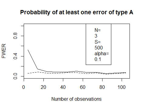
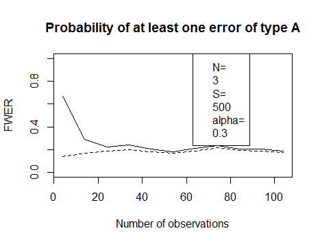
Figure 1: FWER as a function of $n$. N=3. Left: significance level $\alpha=0.1$. Right: significance level $\alpha=0.3$ Solid line - procedure $\delta_{1}$ (standard). Dashed line - procedure $\delta_{2}$ (optimal). Horizontal axe represents the number of observations $n$.

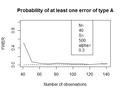
Figure 2: FWER as a function of $n$. N=40. Left: significance level $\alpha=0.1$. Right: significance level $\alpha=0.3$ Solid line - procedure $\delta_{1}$ (standard). Dashed line - procedure $\delta_{2}$ (optimal). Horizontal axe represents the number of observations $n$.

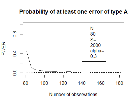
Figure 3: FWER as a function of $n$. N=80. Left: significance level $\alpha=0.1$. Right: significance level $\alpha=0.3$ Solid line - procedure $\delta_{1}$ (standard). Dashed line - procedure $\delta_{2}$ (optimal). Horizontal axe represents the number of observations $n$.

One can note that standard procedure $\delta_{1}$ does not control the FWER for number of observation $n$ close to the matrix dimension $N$. It is interesting to note that FWER for $\delta_{1}$ is rapidly decreasing starting from the value $n=N+1$, it is stabilized from some value of $n=n(N)$ and the difference $(n(N)-N)$ is decreasing in contrast with what one can expect.

7 Concluding remarks

Optimality of individual tests for individual hypotheses testing does not imply in general optimality of associated single-step multiple testing procedure. However if the losses from false decisions are supposed to be additive then in some cases it is possible to prove optimality of multiple testing procedure Lehmann (1957), Koldanov et al (2013). Application of this approach for GGM selection will be a subject of forthcoming publication.

References

• Lauritzen (1996) Lauritzen S.L. (1996). Graphical models. Oxford university press.
• Edwards (2000) Edwards D.(2000). Introduction to graphical modeling. Springer-Verlag New York, Inc.
• Dempster (1972) Dempster A.P.(1972). Covariance selection. Biometrics 28, 157–175.
• Drton and Perlman (2004) Drton M. Perlman M.(2004). Model selection for Gaussian concentration graph. Biometrika 91(3), 591–602.
• Drton and Perlman (2007) Drton M. Perlman M.(2007). Multiple Testing and Error Control in Gaussian Graphical Model Selection. Statistical Science 22(3), 430–449.
• Drton and Perlman (2008) Drton M. Perlman M.(2008). A SINful approach to Gaussian graphical model selection. Journal of Statistical Planning and Inference 138, 1179–1200.
• Anderson (2003) Anderson T. (2003). An introduction to multivariate statistical analysis.3-d edition. Wiley-Interscience, New York.
• Lehmann and Romano (2005) Lehmann E.L. Romano J.P. (2005). Testing statistical hypotheses. 3-d edition. Springer, New York.
• Koldanov and Koldanov (2014) Koldanov A.P. Koldanov P.A. (2014). Optimal multiple decision statistical procedure for inverse covariance matrix. Constructive nonsmooth analysis and related topics, Springer optimization and its applications 87, 205–216.
• Lehmann (1957) Lehmann E.L. (1957). A theory of some multiple decision problems, I. The Annals of Mathematical Statistics, 1-25.
• Koldanov et al (2013) Koldanov A.P., Koldanov P.A., Kalyagin V.A., Pardalos P.M. (2013) Statistical procedures for the market graph construction. Computational Statistics & Data Analysis 68, 17–29, Elsevier.