Reflectivity properties of graphene with nonzero mass-gap parameter

Abstract

The reflectivity properties of graphene with nonzero mass-gap parameter are investigated in the framework of Dirac model using the polarization tensor in (2+1)-dimensional space-time. For this purpose, a more simple explicit representation for the polarization tensor along the real frequency axis is found. The approximate analytic expressions for the polarization tensor and for the reflectivities of graphene are obtained in different frequency regions at any temperature. We show that the nonzero mass-gap parameter has a profound effect on the reflectivity of graphene. Specifically, at zero temperature the reflectivity of gapped graphene goes to zero with vanishing frequency. At nonzero temperature the same reflectivities are equal to unity at zero frequency. We also find the resonance behavior of the reflectivities of gapped graphene at both zero and nonzero temperature at the border frequency determined by the width of the gap. At nonzero temperature the reflectifities of graphene drop to zero in the vicinity of some frequency smaller than the border frequency. Our analytic results are accompanied with numerical computations performed over a wide frequency region. The developed formalism can be used in devising nanoscale optical detectors, optoelectronic switches and in other optical applications of graphene.

I Introduction

Graphene is a two-dimensional sheet of carbon atoms arranged in a hexagonal lattice, which possesses unusual mechanical, electrical and optical properties. At energies below a few eV the electronic excitations (quasiparticles) in graphene are well described by the Dirac model, i.e., display the linear dispersion relation, where the speed of light $c$ is replaced with the Fermi velocity $v_{F}\ll c$ 1 ; 2 . This makes graphene a unique laboratory for testing some effects of quantum electrodynamics and quantum field theory, such as the thermal Casimir force 3 , the Klein paradox 4 , and the creation of particles from vacuum in strong external fields 5 ; 6 ; 7 . It is important also that technological applications of graphene are numerous and diverse. One could mention graphene coatings used in the optical detectors  8 , solar cells 9 , transparent electrodes 10 , corrosium protection 11 , optical biosensors 12 , optoelectronic switches  13 , etc.

In order to make the best use of graphene in both fundamental physics and its applications, it is necessary to investigate the reflectivity properties of this novel material over the wide frequency region. As was shown experimentally, in the region of visible light, where the photon energy is much larger than both thermal and Fermi energies, the transparency and conductivity of graphene are defined by the fine structure constant $\alpha=e^{2}/(\hbar c)$ 14 and by the quantity $e^{2}/(4\hbar)$ 15 , respectively. These facts were understood in theoretical studies of the conductivity of graphene using the current-current correlation function and the Kubo formula (see Ref. 16 and review in Ref. 17 ).

The obtained results for the in-plane (longitudinal) conductivity have been applied to investigate the reflectivity properties of graphene. This was done in the framework of spatially local approximation, i.e., with no regard for dependence on the wave vector. The reflection coefficients and reflectivities of graphene with zero mass-gap parameter (quasiparticle mass) for the transverse magnetic (TM), i.e., $p$ polarized, electromagnetic waves have been found at both low 18 and high 19 frequencies. The case of gapless graphene deposited on a substrate was considered in Ref. 20 .

The most fundamental quantity allowing full investigation of the reflectivity properties of graphene over the entire frequency range is the polarization tensor in (2+1)-dimensional space-time. It was found in Refs. 21 ; 22 at zero and nonzero temperature, respectively, and used to investigate the Casimir effect in graphene systems in Refs. 23 ; 24 ; 25 ; 26 ; 27 ; 28 ; 29 ; 30 (several calculations of the Casimir force were performed also using the density-density correlation functions of graphene and other methods  3 ; 31 ; 32 ; 33 ; 34 ; 35 ). We stress, however, that for calculation of the Casimir force using the Lifshitz theory one should use the reflection coefficients defined at the discrete imaginary Matsubara frequencies  36 ; 37 . It was shown 38 that the polarization tensor of Ref.  22 is valid strictly at the Matsubara frequencies and cannot be immediately continued either to the real or to the entire imaginary frequency axis.

The polarization tensor of graphene valid at all complex frequencies, including the real frequency axis, was derived in Ref. 38 . At the imaginary Matsubara frequencies it coincides with that of Ref. 22 , but, in contrast to Ref. 22 , allows immediate analytic continuation to the whole complex plane. Using this representation for the polarization tensor, the reflectivity properties of gapless graphene were investigated at low, high and intermediate frequencies for both polarizations of the electromagnetic field TM and TE (i.e., transverse electric or $s$ polarization). In so doing, some new properties were found which escaped notice in previous literature. The polarization tensor of Ref. 38 , has been also used to find the reflectivities of material plates coated with gapless graphene 39 .

In this paper, the polarization tensor of Ref. 38 is used to investigate the reflectivity properties of graphene with nonzero mass-gap parameter $m$. It is common knowledge that the quasiparticles of pristine (ideal) graphene are massless. However, they acquire some small mass $m$ under the influence of defects of the structure, electron-electron interaction, and in the presence of substrates 1 ; 40 ; 41 ; 42 ; 43 . The exact value of $m$ for some specific graphene sample usually remains unknown, but, according to some estimations  21 , may achieve 0.1 eV (we measure masses and frequencies in the units of energy). Here, we derive convenient explicit expressions for the polarization tensor of graphene with nonzero mass-gap parameter at any temperature. We demonstrate that under some conditions the nonzero mass-gap parameter may have a dramatic effect on the reflectivity properties of graphene. Specifically, we find the resonance behavior of graphene reflectivities at the border frequency of incident electromagnetic waves $\omega\approx 2mc^{2}/\hbar$. This effect occurs at both zero and nonzero temperature. At nonzero temperature the reflectivities of gapped graphene drop to zero at some frequency smaller than the border one. We find the asymptotic expressions for the reflectivities of gapped graphene at both low and high frequencies. At zero temperature the TM and TE reflectivities of graphene with $m\neq 0$ take the zero value at zero frequency. This is different from the case of gapless graphene, where both reflectivities at zero temperature are equal to nonzero constants depending on $\alpha$ and on the angle of incidence 38 . At nonzero temperature the reflectivities of gapped graphene go to unity with vanishing frequency. We also perform numerical computations of the reflectivities of gapped graphene over the wide range of frequencies at both zero and nonzero temperature and find the regions, where nonzero value of $m$ makes a profound effect on the obtained results.

The paper is organized as follows. In Sec. II we derive convenient expressions for the polarization tensor of graphene with nonzero mass-gap parameter and present the general formalism. Section III contains calculation of the reflectivities of gapped graphene at zero temperature. An investigation of the impact of temperature on the reflectivity of gapped graphene is presented in Sec. IV. In Sec. V the reader will find our conclusions and discussion.

II Special features of the polarization tensor of graphene with nonzero mass-gap parameter

The description of graphene by means of the polarization tensor in (2+1)-dimensional space-time is in fact equivalent 26 to the method using the density-density correlation functions, which is more often used in atomic and condensed matter physics. The formalism of the polarization tensor, however, offers some advantages over the more conventional methods, especially at nonzero temperature, because it has been much studied and elaborated in the framework of thermal quantum field theory.

It is conventional 44 ; 45 to notate the polarization tensor as $\Pi_{\mu\nu}$, where in (2+1)-dimensional case $\mu,\nu=0,1,2$, and $\Pi_{tr}\equiv\Pi_{\mu}^{\mu}$. In our configuration the polarization tensor $\Pi_{\mu\nu}=\Pi_{\mu\nu}(\omega,\theta_{i})$, where $\omega$ is the frequency of electromagnetic wave incident on graphene and $\theta_{i}$ is the angle of incidence. We assume that the graphene sheet is situated in the plane $(x,y)$ and the $z$ azis is perpendicular to it. Then for real photons on a mass-shell the magnitude of the wave vector component parallel to graphene (i.e., perpendicular to the $z$ axis) is defined as

$$k_{\|}=\frac{\omega}{c}\sin\theta_{i}\,.$$ (1)

The amplitude reflection coefficients for TM and TE polarizations of the electromagnetic field incident on a graphene sheet are given by  22 ; 23 ; 24 ; 25 ; 26 ; 27 ; 28 ; 29 ; 30 ; 38

$$r_{\rm TM}(\omega,\theta_{i})=\frac{\cos\theta_{i}\,\Pi_{00}(\omega,\theta_{i})}{2i\hbar\frac{\omega}{c}\sin^{2}\theta_{i}+\cos\theta_{i}\,\Pi_{00}(\omega,\theta_{i})},$$

$$r_{\rm TE}(\omega,\theta_{i})=\frac{\Pi(\omega,\theta_{i})}{2i\hbar\frac{\omega^{3}}{c^{3}}\sin^{2}\theta_{i}\,\cos\theta_{i}-\Pi(\omega,\theta_{i})},$$ (2)

where the following notation is introduced:

$$\Pi(\omega,\theta_{i})=\frac{\omega^{2}}{c^{2}}\left[\sin^{2}\theta_{i}\,\Pi_{\rm tr}(\omega,\theta_{i})+\cos^{2}\theta_{i}\,\Pi_{00}(\omega,\theta_{i})\right]\,.$$ (3)

Note that so important quantity as the conductivity of graphene can be immediately expressed via the polarization tensor. Thus, the spatially nonlocal (i.e., depending on the wave vector) longitudinal and transverse conductivities of graphene are given by 26

$$\sigma_{\|}(\omega,k_{\|})=-i\frac{\omega}{4\pi\hbar k_{\|}^{2}}\,\Pi_{00}(\omega,k_{\|}),\qquad\sigma_{\bot}(\omega,k_{\|})=i\frac{c^{2}}{4\pi\hbar k_{\|}^{2}\omega}\,\Pi(\omega,k_{\|}).$$ (4)

It is convenient to represent the quantities $\Pi_{00}$ and $\Pi$ in the form

$$\Pi_{00}(\omega,\theta_{i})=\Pi_{00}^{(0)}(\omega,\theta_{i})+\Delta_{T}\Pi_{00}(\omega,\theta_{i}),$$

$$\Pi(\omega,\theta_{i})=\Pi^{(0)}(\omega,\theta_{i})+\Delta_{T}\Pi(\omega,\theta_{i}),$$ (5)

where $\Pi^{(0)}_{00}$ and $\Pi^{(0)}$ are defined at zero temperature and $\Delta_{T}\Pi_{00}$, $\Delta_{T}\Pi$ are the thermal corrections which go to zero in the limiting case of vanishing temperature.

The explicit expressions for the quantities $\Pi^{(0)}_{00}$ and $\Pi^{(0)}$ at the imaginary frequencies in the case of arbitrary mass-gap parameter $m$ have been found in Ref. 21 . In our case of real frequencies they can be presented in the form

$$\Pi_{00}^{(0)}(\omega,\theta_{i})=-\frac{\alpha\sin^{2}\theta_{i}}{\eta^{2}(\theta_{i})}\,\Phi(\omega,\theta_{i}),$$

$$\Pi^{(0)}(\omega,\theta_{i})=\alpha\frac{\omega^{2}}{c^{2}}\sin^{2}\theta_{i}\Phi(\omega,\theta_{i}),$$ (6)

where $\eta(\theta_{i})\equiv\eta=[1-\tilde{v}_{F}^{2}\sin^{2}\theta_{i}]^{1/2}$, $\tilde{v}_{F}\equiv v_{F}/c$ and the function $\Phi$ is given by 38

$$\Phi(\omega,\theta_{i})=\left\{\begin{array}[]{ll}4mc-\frac{2\hbar\omega\eta}{c}\left[1+\frac{4m^{2}c^{4}}{\hbar^{2}\omega^{2}\eta^{2}}\right]{\rm arctanh}\frac{\hbar\omega\eta}{2mc^{2}},&\hbar\omega<\frac{2mc^{2}}{\eta},\\[2.84526pt] 4mc-\frac{2\hbar\omega\eta}{c}\left[1+\frac{4m^{2}c^{4}}{\hbar^{2}\omega^{2}\eta^{2}}\right]\left({\rm arctanh}\frac{2mc^{2}}{\hbar\omega\eta}+i\frac{\pi}{2}\right),&\hbar\omega\geq\frac{2mc^{2}}{\eta}.\end{array}\right.$$ (7)

Note that for a gapless graphene ($m=0$) only the second line in Eq. (7) is applicable at all $\omega$. In this case the function $\Phi$ is pure imaginary and has the negative imaginary part

$$\Phi(\omega,\theta_{i})=-i\pi\hbar\frac{\omega}{c}\eta(\theta_{i}).$$ (8)

Substituting Eqs. (6) and  (8) in Eq. (4) with account of Eq. (1), one finds the conductivities of graphene at zero temperature

$$\sigma_{\|}^{(0)}(\omega,k_{\|})=\frac{e^{2}}{4\hbar}\,\frac{\omega}{\sqrt{\omega^{2}-\tilde{v}_{F}^{2}c^{2}k_{\|}^{2}}},\qquad\sigma_{\bot}^{(0)}(\omega,k_{\|})=\frac{e^{2}}{4\hbar}\,\frac{\sqrt{\omega^{2}-\tilde{v}_{F}^{2}c^{2}k_{\|}^{2}}}{\omega},$$ (9)

which are in accordance with the previous knowledge (see, for instance, Refs. 14 ; 15 ; 16 ; 17 ; 46 ).

Now we consider thermal corrections to the 00 component of the polarization tensor and to its trace entering the definition (3) of the quantity $\Pi$. According to Eqs. (33)–(36) of Ref. 38 , along the real frequency axis these thermal corrections can be written in the form

$$\Delta_{T}\Pi_{00({\rm tr})}(\omega,\theta_{i})=\frac{16\alpha\hbar}{\tilde{v}_{F}^{2}}\int_{0}^{\infty}\!\!\!dq\frac{q}{\Gamma(q)}\,\frac{1}{e^{\beta\Gamma(q)}+1}\left[1+\frac{1}{2}\sum_{\lambda=\pm 1}\frac{M_{00({\rm tr})}^{(\lambda)}(\omega,\theta_{i},q)}{N^{(\lambda)}(\omega,\theta_{i},q)}\right],$$ (10)

where $\beta\equiv\hbar c/(k_{B}T)$. Here, the integration variable $q$ has the dimension 1/cm, $\Gamma(q)=[q^{2}+(mc/\hbar)^{2}]^{1/2}$, $k_{B}$ is the Boltzmann constant, $T$ is the temperature, and the following notations are introduced:

$$M_{00}^{(\lambda)}(\omega,\theta_{i},q)=4\Gamma^{2}(q)+\frac{\omega^{2}}{c^{2}}\eta^{2}(\theta_{i})+4\lambda\frac{\omega}{c}\Gamma(q),$$ (11)

$$M_{{\rm tr}}^{(\lambda)}(\omega,\theta_{i},q)=\frac{\omega^{2}}{c^{2}}\eta^{2}(\theta_{i})+4\tilde{v}_{F}^{2}\left(\frac{mc}{\hbar}\right)^{2}+4\left(1-\tilde{v}_{F}^{2}\right)\left[\Gamma^{2}(q)+\lambda\frac{\omega}{c}\Gamma(q)\right].$$

The expression for $N^{(\lambda)}$ depends on the fulfilment of the following conditions:

$$N^{(\lambda)}(\omega,\theta_{i},q)=\left\{\begin{array}[]{ll}{\rm sign}Q_{\lambda}\left[{Q_{\lambda}}^{\!\!\!2}-\left(2\tilde{v}_{F}\frac{\omega}{c}q\sin\theta_{i}\right)^{2}\right]^{1/2},&|Q_{\lambda}|\geq 2\tilde{v}_{F}\frac{\omega}{c}q\sin\theta_{i},\\[2.84526pt] -i\left[-{Q_{\lambda}}^{\!\!\!2}+\left(2\tilde{v}_{F}\frac{\omega}{c}q\sin\theta_{i}\right)^{2}\right]^{1/2},&|Q_{\lambda}|<2\tilde{v}_{F}\frac{\omega}{c}q\sin\theta_{i},\end{array}\right.$$ (12)

where

$$Q_{\lambda}\equiv Q_{\lambda}(\omega,\theta_{i},q)=-\frac{\omega^{2}}{c^{2}}\eta^{2}(\theta_{i})-2\lambda\frac{\omega}{c}\Gamma(q).$$ (13)

In the case of $m\neq 0$ under consideration here it is more convenient to represent the temperature correction  (10) as an integral with respect to the new variable $u=\Gamma(q)$:

$$\Delta_{T}\Pi_{00({\rm tr})}(\omega,\theta_{i})=\frac{16\alpha\hbar}{\tilde{v}_{F}^{2}}\int_{mc/\hbar}^{\infty}\!\!\!du\frac{1}{e^{\beta u}+1}\left[1+\frac{1}{2}\sum_{\lambda=\pm 1}\frac{M_{00({\rm tr})}^{(\lambda)}(\omega,\theta_{i},u)}{N^{(\lambda)}(\omega,\theta_{i},u)}\right],$$ (14)

where

$$M_{00}^{(\lambda)}(\omega,\theta_{i},u)=4u^{2}+\frac{\omega^{2}}{c^{2}}\eta^{2}(\theta_{i})+4\lambda\frac{\omega}{c}u,$$ (15)

$$M_{{\rm tr}}^{(\lambda)}(\omega,\theta_{i},u)=\frac{\omega^{2}}{c^{2}}\eta^{2}(\theta_{i})+4\tilde{v}_{F}^{2}\left(\frac{mc}{\hbar}\right)^{2}+4\left(1-\tilde{v}_{F}^{2}\right)\left(u^{2}+\lambda\frac{\omega}{c}u\right).$$

The quantity $Q_{\lambda}$ defined in Eq. (13) takes the form

$$Q_{\lambda}\equiv Q_{\lambda}(\omega,\theta_{i},u)=-\frac{\omega^{2}}{c^{2}}\eta^{2}(\theta_{i})-2\lambda\frac{\omega}{c}u.$$ (16)

It is easily seen that for $\lambda=1$ the quantity $Q_{\lambda}$ is always negative and satisfies the condition

$$|Q_{1}|\geq 2\tilde{v}_{F}\frac{\omega}{c}\left[u^{2}-\left(\frac{mc}{\hbar}\right)^{2}\right]^{1/2}\sin\theta_{i}\,.$$ (17)

Thus, the first line in Eq. (12) is applicable leading to

$$N^{(1)}(\omega,\theta_{i},u)=-\frac{\omega}{c}\left\{\vphantom{\left[4\left(\frac{mc}{\hbar}\right)^{2}-\frac{\omega^{2}}{c^{2}}\eta^{2}(\theta_{i})\right]}\eta^{2}(\theta_{i})\left(\frac{\omega}{c}+2u\right)^{2}+\tilde{v}_{F}^{2}\sin^{2}\theta_{i}\left[4\left(\frac{mc}{\hbar}\right)^{2}-\frac{\omega^{2}}{c^{2}}\eta^{2}(\theta_{i})\right]\right\}^{1/2}.$$ (18)

The case $\lambda=-1$ is more complicated and deserves separate consideration. According to Eq. (16) in this case $Q_{-1}$ can be both positive and negative. In order to explicitly rewrite Eq. (12) in terms of the variable $u$, we introduce the quantity

$$\chi(\omega,\theta_{i},u)\equiv{Q^{\,2}_{-1}}-4\tilde{v}_{F}^{2}\frac{\omega^{2}}{c^{2}}\left[u^{2}-\left(\frac{mc}{\hbar}\right)^{2}\right]\sin^{2}\theta_{i}$$ (19)

$$~{}~{}=\frac{\omega^{2}}{c^{2}}\left\{\vphantom{\left[4\left(\frac{mc}{\hbar}\right)^{2}-\frac{\omega^{2}}{c^{2}}\eta^{2}(\theta_{i})\right]}\eta^{2}(\theta_{i})\left(\frac{\omega}{c}-2u\right)^{2}+\tilde{v}_{F}^{2}\sin^{2}\theta_{i}\left[4\left(\frac{mc}{\hbar}\right)^{2}-\frac{\omega^{2}}{c^{2}}\eta^{2}(\theta_{i})\right]\right\}.$$

The sign of the quantity $\chi$ under different values of parameters is found by solving the equation

$$\chi(\omega,\theta_{i},u)=0$$ (20)

with respect to the variable $u$:

$$u^{(\pm)}=\frac{1}{2}\left[\frac{\omega}{c}\pm\tilde{v}_{F}\sin\theta_{i}\sqrt{\frac{\omega^{2}}{c^{2}}-\frac{4m^{2}c^{2}}{\hbar^{2}\eta^{2}(\theta_{i})}}\right].$$ (21)

If the condition

$$\omega<\frac{2mc^{2}}{\hbar\eta(\theta_{i})}$$ (22)

is satisfied, Eq. (20) does not possess real roots and the function $\chi$ is always positive. In this case the first line in Eq. (12) is applicable and

$$N_{-1}(\omega,\theta_{i},u)=\sqrt{\chi(\omega,\theta_{i},u)},\quad\frac{mc}{\hbar}\leq u<\infty,$$ (23)

where $\chi$ is defind in Eq. (19).

Now we consider the opposite condition

$$\omega\geq\frac{2mc^{2}}{\hbar\eta(\theta_{i})},$$ (24)

when Eq. (20) has two different real roots $u^{(\pm)}$ defined in Eq. (21) [they coincide in the case of equality in Eq. (24)]. It is easily seen that under the condition (24) $u^{(-)}\geq mc/\hbar$. Thus, in the regions $mc/\hbar\leq u\leq u^{(-)}$ and $u\geq u^{(+)}$ the function $\chi$ is nonnegative and the quantity $N^{(-1)}$ is given by the first line of Eq. (12). In so doing $Q_{-1}>0$ in the latter interval whereas it can be both negative and positive in the former. As to the region $u^{(-)}<u<u^{(+)}$, here the function $\chi$ is negative and, as a consequence, $N^{(-1)}$ is given by the second line of Eq. (12). Combining all these facts together, for the quantity $N^{(-1)}$ one obtains

$$N^{(-1)}(\omega,\theta_{i},u)=\left\{\begin{array}[]{ll}{\rm sign}Q_{-1}\sqrt{\chi(\omega,\theta_{i},u)},&\frac{mc}{\hbar}\leq u\leq u^{(-)},\\ -i\sqrt{-\chi(\omega,\theta_{i},u)},&u^{(-)}<u<u^{(+)},\\ \sqrt{\chi(\omega,\theta_{i},u)},&u\geq u^{(+)}.\end{array}\right.$$ (25)

Simple analysis using Eqs. (13) and (21) shows that for $u\leq u^{(-)}$ within the interval

$$\frac{2mc^{2}}{\hbar\eta(\theta_{i})}\leq\omega<\frac{2mc^{2}}{\hbar\eta^{2}(\theta_{i})}$$ (26)

we have ${\rm sign}Q_{-1}=+1$, whereas within the interval

$$\omega>\frac{2mc^{2}}{\hbar\eta^{2}(\theta_{i})}$$ (27)

it holds ${\rm sign}Q_{-1}=-1$.

Equations (14)–(16), (18), (19), (23) and (25) are convenient for both analytic and numerical calculations using the polarization tensor of gapped graphene. To apply them for calculations of the reflection coefficients and reflectivities, it is convenient also to present an explicit expression for the quantity $\Delta_{T}\Pi(\omega,\theta_{i})$. It is obtained from Eqs. (3), (14) and (15) and has the form

$$\Delta_{T}\Pi(\omega,\theta_{i})=\frac{16\alpha\hbar}{\tilde{v}_{F}^{2}}\int_{mc/\hbar}^{\infty}\!\!\!du\frac{1}{e^{\beta u}+1}\left[\frac{\omega^{2}}{c^{2}}+\frac{1}{2}\sum_{\lambda=\pm 1}\frac{M^{(\lambda)}(\omega,\theta_{i},u)}{N^{(\lambda)}(\omega,\theta_{i},u)}\right],$$ (28)

where the quantity $M^{(\lambda)}$ is given by

$$M^{(\lambda)}(\omega,\theta_{i},u)=\frac{\omega^{2}}{c^{2}}\left[\eta^{2}(\theta_{i})\left(2u+\lambda\frac{\omega}{c}\right)^{2}+4\tilde{v}_{F}^{2}\left(\frac{mc}{\hbar}\right)^{2}\sin^{2}\theta_{i}\right].$$ (29)

The denominator $N^{(\lambda)}$ in Eq. (28) is presented in Eqs. (18) and (25). In the limiting case $m\to 0$ the above expressions take a more simple form used in Ref. 38 to investigate the reflectivity properties of gapless graphene.

III Reflectivity of gapped graphene at zero temperature

At $T=0$ the polarization tensor of graphene is given by Eqs. (6) and (7). We consider first the region of frequencies (22). Here, the first line of Eq. (7) is applicable which can be rewritten in the form

$$\Phi(\omega,\theta_{i})=4mc\left[1-\frac{2mc^{2}}{\hbar\omega\eta}\left(1+\frac{\hbar^{2}\omega^{2}\eta^{2}}{4m^{2}c^{4}}\right){\rm arctanh}\frac{\hbar\omega\eta}{2mc^{2}}\right].$$ (30)

This is real function in contrast with the case of gapless graphene [in the latter case the function $\Phi$ is pure imaginary, see Eq. (8)].

Substituting Eq. (6) with the real function $\Phi$ in Eq. (2), one obtains the reflection coefficients and reflectivities of gapped graphene at sufficiently low frequencies

$${\cal R}_{\rm TM}(\omega,\theta_{i})\equiv|r_{\rm TM}(\omega,\theta_{i})|^{2}=\frac{\alpha^{2}\cos^{2}(\theta_{i})\Phi^{2}(\omega,\theta_{i})}{4\hbar^{2}\frac{\omega^{2}}{c^{2}}\eta^{4}(\theta_{i})+\alpha^{2}\cos^{2}(\theta_{i})\Phi^{2}(\omega,\theta_{i})},$$

$${\cal R}_{\rm TE}(\omega,\theta_{i})\equiv|r_{\rm TE}(\omega,\theta_{i})|^{2}=\frac{\alpha^{2}\Phi^{2}(\omega,\theta_{i})}{4\hbar^{2}\frac{\omega^{2}}{c^{2}}\cos^{2}(\theta_{i})+\alpha^{2}\Phi^{2}(\omega,\theta_{i})},$$ (31)

where $\Phi$ is defined by Eq. (30). It is seen that at the normal incidence ($\theta_{i}=0$)

$${\cal R}_{\rm TM}(\omega,0)={\cal R}_{\rm TE}(\omega,0),$$ (32)

as it should be.

III.1 Asymptotic results

Now we consider the asymptotic regime of very small frequencies satisfying the condition

$$\frac{\hbar\omega\eta(\theta_{i})}{2mc^{2}}\ll 1.$$ (33)

Expanding Eq. (30) in powers of small parameter (33), one obtains

$$\Phi(\omega,\theta_{i})\approx-\frac{4\hbar^{2}\omega^{2}\eta^{2}(\theta_{i})}{3mc^{3}}.$$ (34)

Substituting this in Eq. (31) with account of Eq. (33), we arrive at

$${\cal R}_{\rm TM}(\omega,\theta_{i})\approx\frac{4}{9}\alpha^{2}\cos^{2}(\theta_{i})\frac{\hbar^{2}\omega^{2}}{m^{2}c^{4}},\qquad{\cal R}_{\rm TE}(\omega,\theta_{i})\approx\frac{4\alpha^{2}\hbar^{2}\omega^{2}}{9m^{2}c^{4}\cos^{2}(\theta_{i})}.$$ (35)

Note that in Eq. (35) and below we have also used $\eta(\theta_{i})\approx 1$.

As can be seen in Eq. (35),

$${\cal R}_{\rm TM}(\omega,\theta_{i}),{\ }{\cal R}_{\rm TE}(\omega,\theta_{i})\to 0{\ \ }\mbox{when}{\ }\omega\to 0.$$ (36)

This is different from the case of gapless graphene at zero temperature. In the latter case, substituting Eq. (8) in Eq. (6), one finds

$$\Pi_{00}^{(0)}(\omega,\theta_{i})=i\alpha\pi\hbar\frac{\omega}{c}\,\sin^{2}\theta_{i},\qquad\Pi^{(0)}(\omega,\theta_{i})=-i\alpha\pi\hbar\frac{\omega^{3}}{c^{3}}\,{\sin^{2}\theta_{i}}.$$ (37)

Substituting these equations in Eq. (2), after simple calculation, we obtain

$${\cal R}_{\rm TM}(\theta_{i})=\frac{\alpha^{2}\pi^{2}\cos^{2}\theta_{i}}{(\alpha\pi\cos\theta_{i}+2)^{2}},\qquad{\cal R}_{\rm TE}(\theta_{i})=\frac{\alpha^{2}\pi^{2}}{(2\cos\theta_{i}+\alpha\pi)^{2}}.$$ (38)

Note that both reflectivities in Eq. (38) do not depend on the frequency and, thus, take nonzero values at $\omega=0$, as opposed to Eq. (36) for a gapped graphene.

We are coming now to the asymptotic region

$$\omega\to\frac{2mc^{2}}{\hbar\eta(\theta_{i})},$$ (39)

where the quantity on the left-hand side of Eq. (33) approaches unity from the left. It is convenient to present the frequency in the form

$$\omega=\frac{2mc^{2}}{\hbar\eta(\theta_{i})}\left(1-2e^{-\tau}\right),$$ (40)

where the limiting case (39) corresponds to $\tau\to\infty$.

Substituting Eq. (40) in Eq. (30), one finds that at $\tau\to\infty$

$$\Phi(\omega,\theta_{i})\approx 4mc(1-\tau)\approx-4mc\tau.$$ (41)

Then from Eq. (31) we conclude that in the limiting case (39)

$${\cal R}_{\rm TM}(\omega,\theta_{i})\to 1,\quad{\cal R}_{\rm TE}(\omega,\theta_{i})\to 1.$$ (42)

The next region to consider is given by Eq. (24). Here, the second line of Eq. (7) is applicable, where the function $\Phi$ has both real and imaginary parts

$${\rm Re}\Phi(\omega,\theta_{i})=4\left[mc-\frac{\hbar\omega\eta}{2c}\left(1+\frac{4m^{2}c^{4}}{\hbar^{2}\omega^{2}\eta^{2}}\right){\rm arctanh}\frac{2mc^{2}}{\hbar\omega\eta}\right],$$

$${\rm Im}\Phi(\omega,\theta_{i})=-\frac{\pi\hbar\omega\eta}{c}\left(1+\frac{4m^{2}c^{4}}{\hbar^{2}\omega^{2}\eta^{2}}\right).$$ (43)

Using Eqs. (2) and (6), we find the reflectivities in the form

$${\cal R}_{\rm TM}(\omega,\theta_{i})=\frac{\alpha^{2}\cos^{2}(\theta_{i})[{\rm Re}^{2}\Phi(\omega,\theta_{i})+{\rm Im}^{2}\Phi(\omega,\theta_{i})]}{\alpha^{2}\cos^{2}(\theta_{i}){\rm Re}^{2}\Phi(\omega,\theta_{i})+\left[2\hbar\frac{\omega}{c}\eta^{2}-\alpha\cos\theta_{i}{\rm Im}\Phi(\omega,\theta_{i})\right]^{2}},$$

$${\cal R}_{\rm TE}(\omega,\theta_{i})=\frac{\alpha^{2}[{\rm Re}^{2}\Phi(\omega,\theta_{i})+{\rm Im}^{2}\Phi(\omega,\theta_{i})]}{\alpha^{2}{\rm Re}^{2}\Phi(\omega,\theta_{i})+\left[2\hbar\frac{\omega}{c}\cos\theta_{i}-\alpha{\rm Im}\Phi(\omega,\theta_{i})\right]^{2}}.$$ (44)

Now we consider the asymptotic behavior of the reflectivities at high frequencies

$$\frac{\hbar\omega\eta(\theta_{i})}{2mc^{2}}\gg 1.$$ (45)

In this case Eq. (43) leads to

$${\rm Re}\Phi(\omega,\theta_{i})\approx-\frac{64m^{3}c^{5}}{3\hbar^{2}\omega^{2}\eta^{2}(\theta_{i})}\to 0{\ \ }\mbox{when}{\ }\omega\to\infty,$$

$${\rm Im}\Phi(\omega,\theta_{i})\approx-\pi\hbar\frac{\omega}{c}\eta(\theta_{i}),$$ (46)

i.e., to the same result as for a gapless graphene [see Eq. (8)]. Then, the reflectrivities are again given by Eq. (38) or, neglecting by the small terms, as compared to unity, by

$${\cal R}_{\rm TM}(\theta_{i})\approx\frac{\alpha^{2}\pi^{2}\cos^{2}\theta_{i}}{(2+\alpha\pi\cos\theta_{i})^{2}},\qquad{\cal R}_{\rm TE}(\theta_{i})\approx\frac{\alpha^{2}\pi^{2}}{(2\cos\theta_{i}+\alpha\pi)^{2}}.$$ (47)

Note that these reflectivities do not depend on the frequency and on the mass-gap parameter.

The remaining asymptotic region is given by Eq. (39) when the quantity on the left-hand side of Eq. (45) approaches unity from the right. In this case from the second line of Eq. (43) one obtains

$${\rm Im}\Phi(\omega,\theta_{i})\approx-2\pi\hbar\frac{\omega}{c}\eta(\theta_{i}).$$ (48)

The asymptotic behavior of the real part of $\Phi$ in the first line of Eq. (43) can be found similar to Eqs. (40) and (41) with the same results for the reflectivity properties as in Eq. (42).

III.2 Numerical computations

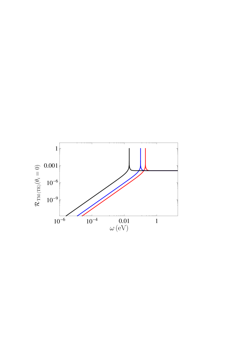
Figure 1: (Color online) The reflectivity of gapped graphene at $T=0\,$K at the normal incidence is shown as a function of frequency by the three lines from right to left for the mass-gap parameter $m$=0.1, 0.05, and 0.01 eV, respectively.

We are coming to numerical computations of the reflectivity properties of gapped graphene at zero temperature over wide frequency range of incident electromagnetic waves. Computations are performed by using Eqs. (2), (6) and (7). Taking into account that due to the conditions $\tilde{v}_{F}\ll 1$, $\eta\approx 1$ the angular dependences of reflectivities are similar to those for gapless graphene 38 , computations are performed at the normal incidence. In Fig. 1 the three lines from right to left show the computational results for the TM and TE reflectivities (32) at the normal incidence calculated as functions of frequency for the graphene sheets with mass-gap parameter $m$ equal to 0.1, 0.05, and 0.01 eV, respectively. The double logarithmic scale is used allowing to cover the frequency range from 1 $\mu$eV to 20 eV. The linear dependence of the logarithm of reflectivities on the logarithm of frequency at low frequencies satisfying the condition (33) corresponds to the asymptotic regime where Eq. (35) is applicable. At the frequency value

$$\omega=\frac{2mc^{2}}{\hbar},$$ (49)

which is different for different $m$ [recall that at the normal incidence $\eta(0)=1$], the narrow resonances are observed in Fig. 1. Under the condition (39) these resonances satisfy Eq. (42). At high frequencies satisfying the condition (45) the asymptotic equations (47) are applicable. Note that at $\theta_{i}=0$ one can neglect by $\alpha\pi$, as compared with 2 in the denominators.

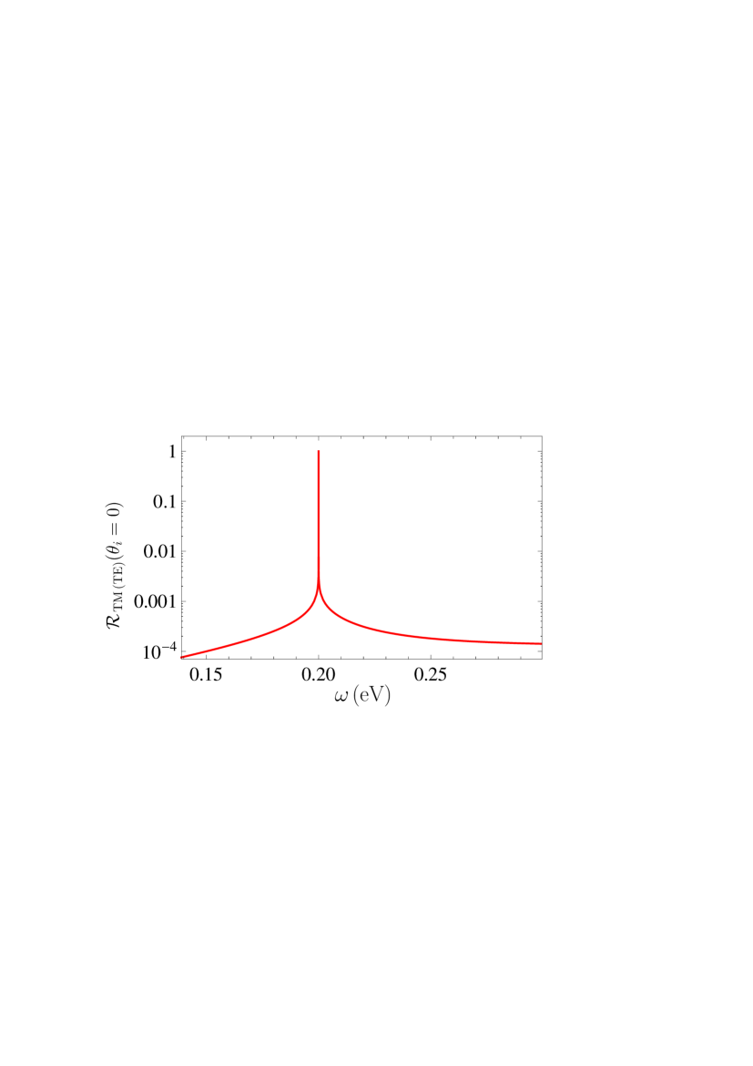
Figure 2: (Color online) The reflectivity of graphene with the mass-gap parameter $m$=0.1 eV at $T=0\,$K at the normal incidence is shown as a function of frequency in the vicinity of the resonance frequency $\omega=2mc^{2}/\hbar$.

It would be interesting to investigate in more detail an immediate vicinity of the resonance frequency (49), where the above asymptotic expressions do not apply. As an example, in Fig. 2 we again plot the reflectivity at the normal incidence (32) as a function of frequency for the graphene sheet with $m=0.1\,eV$. Now the computational results are plotted over a narrow frequency region from 0.14 to 0.30 eV using the natural scale in the frequency axis. As is seen in Fig. 2, even over a so narrow range, the reflectivity of graphene varies by four orders of magnitude, whereas the width of the resonance peak remains unresolved.

In fact the half-width of this resonance can be found analytically from the asymptotic representation (41). Substituting Eq. (41) in Eq. (31) taken at $\theta_{i}=0$, we find

$${\cal R}_{\rm TM}(\omega,0)={\cal R}_{\rm TM}(\omega,0)\approx\frac{\alpha^{2}\tau^{2}}{\frac{\hbar^{2}\omega^{2}}{4m^{2}c^{4}}+\alpha^{2}\tau^{2}}.$$ (50)

Taking into account Eq. (49), one obtains that ${\cal R}_{\rm TM\,(TE)}\approx 1/2$ when $\alpha^{2}\tau^{2}=1$, i.e., for $\tau=1/\alpha\approx 137$. Then, using Eq. (40), we conclude that the half-width of the resonance is equal to

$$4e^{-137}\frac{mc^{2}}{\hbar}\sim 10^{-59}\frac{mc^{2}}{\hbar}.$$ (51)

This half-width is too small and makes the resonance under consideration unobservable. However, at zero temperature it might be possible to observe the change in the reflectivity of graphene by a factor of ten with increasing frequency of the incident light. Thus, the reflectivity increases from 0.00013 to 0.00134 when $\omega$ increases from 0.16 to 0.199 eV. In a similar way, with further increase of frequency from 0.201 to 0.3 eV the reflectivity of graphene changes from 0.00141 to 0.000141.

We consider now more detailly the region of frequencies from 0 to 0.4 eV, where the reflectivity varies by more than an order of magnitude for all values of $m$ under discussion. Note that at room temperature ($T=300\,$K) it holds $k_{B}T\approx 0.025$ eV, i.e., the thermal energy is of the same order as $mc^{2}$ for the smallest value of $m$.

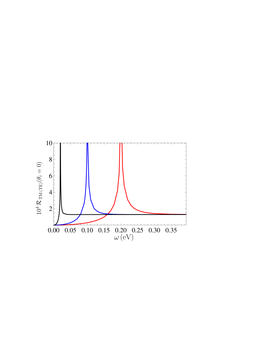
Figure 3: (Color online) The reflectivity of gapped graphene at $T=0\,$K at the normal incidence is shown as a function of frequency using the natural scales in the vicinity of resonance frequencies. The three lines from right to left are for the mass-gap parameter $m$=0.1, 0.05, and 0.01 eV, respectively.

In Fig. 3 we plot the reflectivity of gapped graphene at the normal incidence as a function of frequency by the three lines from right to left for the mass-gap parameter $m=0.1$, 0.05, and 0.01 eV, respectively. In this figure, both the reflectivity and frequency are plotted in their natural scales. Because of this, only the lower parts of the resonance peaks are shown. As is seen in Fig. 3, an impact of the mass-gap parameter of graphene on the reflectivity properties decreases with decreasing $m$ and increasing frequency. For small mass-gap parameters $m<0.01$ eV in the region $\hbar\omega>2mc^{2}$ the reflectivity is approximately equal to that obtained for $m=0$ at any temperature $T\leq 300$ K 38 . The role of nonzero temperature in the case of gapped graphene is considered below.

IV Influence of nonzero temperature on the reflectivity of gapped graphene

In this section, we consider the reflection coefficients (2), where the quantities $\Pi_{00}$ and $\Pi$ are given by Eq. (5), i.e., are defined at any nonzero temperature. In so doing, the zero-temperature contributions are presented in Eqs. (6) and (7) and the thermal corrections to them are given in Eqs. (14) and (28) with all necessary notations in Eqs. (15)–(19), (23), (25) and (29).

IV.1 Asymptotic results

We begin with thermal correction to the polarization tensor of graphene calculated at frequencies satisfying Eq. (22). From Eqs. (14), (15), (18), (19) and (23) one obtains

$$\Delta_{T}\Pi_{00}(\omega,\theta_{i})=\frac{16\alpha\hbar}{\tilde{v}_{F}^{2}}\int_{mc/\hbar}^{\infty}\frac{du}{e^{\beta u}+1}\left\{\vphantom{\left[\frac{(2cu-\omega)^{2}-\tilde{v}_{F}^{2}\omega^{2}\sin^{2}\theta_{i}}{\sqrt{(2cu-\omega)^{2}+\tilde{v}_{F}^{2}\omega^{2}\left(\frac{4m^{2}c^{4}}{\hbar^{2}\omega^{2}\eta^{2}}-1\right)\sin^{2}\theta_{i}}}\right]}1+\frac{1}{2\omega\eta}\right.$$

$$\times\left[-\frac{(2cu+\omega)^{2}-\tilde{v}_{F}^{2}\omega^{2}\sin^{2}\theta_{i}}{\sqrt{(2cu+\omega)^{2}+\tilde{v}_{F}^{2}\omega^{2}\left(\frac{4m^{2}c^{4}}{\hbar^{2}\omega^{2}\eta^{2}}-1\right)\sin^{2}\theta_{i}}}\right.$$

(52)

$$+\left.\left.\frac{(2cu-\omega)^{2}-\tilde{v}_{F}^{2}\omega^{2}\sin^{2}\theta_{i}}{\sqrt{(2cu-\omega)^{2}+\tilde{v}_{F}^{2}\omega^{2}\left(\frac{4m^{2}c^{4}}{\hbar^{2}\omega^{2}\eta^{2}}-1\right)\sin^{2}\theta_{i}}}\right]\right\}.$$

Now we impose a more stringent than Eq. (22) requirement, i.e., $\hbar\omega\lesssim mc^{2}$.Under this requirement the quantity $2cu-\omega$ cannot become too small and one can expand both square roots in Eq. (52) up to the first order of respective small parameters with the result

$$\Delta_{T}\Pi_{00}(\omega,\theta_{i})\approx\frac{16\alpha\hbar}{\tilde{v}_{F}^{2}}\int_{mc/\hbar}^{\infty}\frac{du}{e^{\beta u}+1}$$ (53)

$$~{}~{}\times\left\{1+\frac{1}{2\eta}\left[-2+\frac{\tilde{v}_{F}^{2}\sin^{2}\theta_{i}}{2}\left(\frac{4m^{2}c^{4}}{\hbar^{2}\omega^{2}\eta^{2}}+1\right)\left(\frac{\omega}{2cu+\omega}-\frac{\omega}{2cu-\omega}\right)\right]\right\}.$$

Then, using the smallness of $\tilde{v}_{F}$, we arrive at

$$\Delta_{T}\Pi_{00}(\omega,\theta_{i})\approx-8\alpha\hbar\sin^{2}\theta_{i}\int_{mc/\hbar}^{\infty}\frac{du}{e^{\beta u}+1}\left(1+\frac{4\frac{m^{2}c^{4}}{\hbar^{2}}+\omega^{2}}{4u^{2}c^{2}-\omega^{2}}\right).$$ (54)

Note that Eq. (54) is also valid under a less stringent condition (22) if one assumes that $\hbar\omega\ll k_{B}T$. This is because the main contribution to the integral in Eq. (52) is given by $\hbar cu\sim k_{B}T$ and hence the quantity $2cu-\omega$ cannot become too small. Both application regions of Eq. (54) are used below to obtain approximate expressions for the polarization tensor and reflectivity of gapped graphene at nonzero temperature.

It is convenient to introduce two dimensionless parameters and new integration variable according to

$$\mu\equiv\frac{mc^{2}}{k_{B}T},\quad\nu\equiv\frac{\hbar\omega}{k_{B}T},\quad v=\frac{\hbar cu}{k_{B}T}\equiv\beta u.$$ (55)

Then Eq. (54) takes the form

$$\Delta_{T}\Pi_{00}(\omega,\theta_{i})\approx-8\alpha\sin^{2}\theta_{i}\frac{k_{B}T}{c}\int_{\mu}^{\infty}\frac{dv}{e^{v}+1}\left(1+\frac{4\mu^{2}+\nu^{2}}{4v^{2}-\nu^{2}}\right).$$ (56)

We consider, first, Eq. (56) under its validity condition $\nu\ll 1$ and assume that $\mu\ll 1$ as well. Taking into account that the main contribution to the integral in Eq. (56) is given by $v\sim 1$, one can neglect by the small second term in the round brackets. Then, after the integration, we arrive at

$$\Delta_{T}\Pi_{00}(\omega,\theta_{i})\approx-8\alpha\frac{k_{B}T}{c}\sin^{2}\theta_{i}\ln\left(1+e^{-\mu}\right)\approx-8\alpha\ln 2\frac{k_{B}T}{c}\sin^{2}\theta_{i}.$$ (57)

The latter thermal correction does not depend on $m$ and coincides with that obtained in Eq. (89) of Ref. 38 for a gapless graphene. Note, however, that for a gapped graphene at $T=0\,$K from Eqs. (6) and (34), i.e., in the case of small frequencies, one obtains

$$\Pi_{00}^{(0)}(\omega,\theta_{i})\approx\frac{4}{3}\alpha\sin^{2}\theta_{i}\frac{\hbar^{2}\omega^{2}}{mc^{3}}.$$ (58)

This is real quantity, as opposed to the case of $m=0$, where $\Pi_{00}^{(0)}$ at small frequencies is pure imaginary.

As is seen using Eq. (22) and the conditions $\mu,\,\nu\ll 1$, $\Pi_{00}^{(0)}\ll\Delta_{T}\Pi_{00}$. As a result, for the TM reflectivity of graphene from Eqs. (2) and (57) we find

$${\cal R}_{\rm TM}(\omega,\theta_{i})\approx\frac{16\alpha^{2}\ln^{2}{2}(k_{B}T)^{2}\cos^{2}\theta_{i}}{\hbar^{2}\omega^{2}+16\alpha^{2}\ln^{2}{2}(k_{B}T)^{2}\cos^{2}\theta_{i}}.$$ (59)

Similar approximate calculation with account of Eqs. (6) and (34) results in

$$\Delta_{T}\Pi(\omega,\theta_{i})\approx 8\alpha\ln 2\frac{\omega^{2}}{c^{2}}\frac{k_{B}T}{c}\sin^{2}\theta_{i}\gg|\Pi^{(0)}(\omega,\theta_{i})|.$$ (60)

Then, substituting this equation in Eq. (2), one obtains

$${\cal R}_{\rm TE}(\omega,\theta_{i})\approx\frac{16\alpha^{2}\ln^{2}{2}(k_{B}T)^{2}}{\hbar^{2}\omega^{2}\cos^{2}\theta_{i}+16\alpha^{2}\ln^{2}{2}(k_{B}T)^{2}}.$$ (61)

Unlike the case of gapped graphene at zero temperature, Eqs. (59) and (61) result in

$${\cal R}_{\rm TM\,(TE)}(\omega,\theta_{i})\to 1{\ \ }\mbox{when}{\ }{\omega\to 0}$$ (62)

similar to the case of gapless graphene at nonzero $T$ 38 . Below we demonstrate, both analytically and numerically, that this is general property of the reflectivity of gapped graphene at $T\neq 0$.

Now we return to Eq. (56) derived under the condition $\hbar\omega\lesssim mc^{2}$ and consider it under additional assumptions $\mu\gg 1$ and $\hbar\omega\ll mc^{2}$. Under these assumptions one can neglect by unity, as compared with $e^{v}$, and by $\nu^{2}$, as compared with $\mu^{2}$ and $v^{2}$. As a result, Eq. (56) takes the form

$$\Delta_{T}\Pi_{00}(\omega,\theta_{i})\approx-8\alpha\sin^{2}\theta_{i}\frac{k_{B}T}{c}\int_{\mu}^{\infty}\!\!\!{dv}{e^{-v}}\left(1+\frac{\mu^{2}}{v^{2}}\right)$$

(63)

$$~{}=-8\alpha\sin^{2}\theta_{i}\frac{k_{B}T}{c}\left\{e^{-\mu}+\mu^{2}\left[\frac{e^{-\mu}}{\mu}+{\rm Ei}(-e^{-\mu})\right]\right\},$$

where ${\rm Ei}(z)$ is the exponential integral. Taking into account the asymptotic expansion 47

$${\rm Ei}(-x)=e^{-x}\left[-\frac{1}{x}+\frac{1}{x^{2}}+O\left(\frac{1}{x^{3}}\right)\right],$$ (64)

one arrives at

$$\Delta_{T}\Pi_{00}(\omega,\theta_{i})\approx-16\alpha\sin^{2}\theta_{i}\frac{k_{B}T}{c}e^{-mc^{2}/(k_{B}T)}.$$ (65)

Combining this expression with Eq. (58), we find

$$\Pi_{00}(\omega,\theta_{i})\approx 4\alpha\sin^{2}\theta_{i}\frac{\omega}{c}\left[\frac{1}{3}\,\frac{\hbar^{2}\omega}{mc^{2}}-4\frac{k_{B}T}{\omega}e^{-mc^{2}/(k_{B}T)}\right],$$ (66)

i.e., the thermal correction is exponentially small. Substituting this equation [and similar for $\Pi(\omega,\theta_{i})$] in Eq. (2), we again obtain Eq. (62) in the limiting case of vanishing frequency.

As is seen from Eq. (66), the thermal correction to the 00 component of the polarization tensor is negative, whereas the zero-temperature contribution to it is positive. Taking into account that they can be of the same order of magnitude, we find the value of frequency $\omega_{0}$ where the quantity $\Pi_{00}$ vanishes

$$\omega_{0}^{2}=12\frac{mc^{2}}{\hbar^{2}}k_{B}Te^{-mc^{2}/(k_{B}T)}.$$ (67)

At room temperature ($k_{B}T=0.025\,$eV) only the maximum value of the mass-gap parameter under consideration here ($m=0.1\,$eV) leads to $\mu=4$ and can be considered as close to the application region of the approximation used. For these values of parameters we find from Eq. (67) the value $\omega_{0}=0.0234\,$eV, which is more or less in agreement with the second application condition of our approximation ($\hbar\omega\ll mc^{2}$). Below we compare the obtained approximate value of $\omega_{0}$ with the results of numerical computations and find rather good agreement. Just now we only note that vanishing of $\Pi_{00}(\omega_{0},\theta_{i})$ leads in accordance with Eq. (2) to vanishing of the reflectivities of graphene ${\cal R}_{\rm TM\,(TE)}(\omega_{0},\theta_{i})$ at the frequency $\omega_{0}\neq 0$. This does not happen either for a gapless graphene at any temperature or for a gapped graphene at $T=0\,$K. In the next subsection we consider the effect of vanishing reflectivity of graphene in more details by means of numerical computations.

Here, we continue with the approximate analytic expressions for the polarization tensor and consider the frequency region of higher frequencies defined in Eq. (24). We start with the imaginary part of the thermal correction (14) which arises only for $\lambda=-1$ and is obtained from the first line of Eq. (15) and the second line of Eq. (25):

$${\rm Im}\Delta_{T}\Pi_{00}(\omega,\theta_{i})=\frac{8\alpha\hbar}{\tilde{v}_{F}^{2}}\int_{u^{(-)}}^{u^{(+)}}\frac{du}{e^{\beta u}+1}\frac{\left(2cu-\omega\right)^{2}-\tilde{v}_{F}^{2}\omega^{2}\sin^{2}\theta_{i}}{\omega\eta\sqrt{\tilde{v}_{F}^{2}\omega^{2}\sin^{2}\theta_{i}\,A(\omega,\theta)-\left(2cu-\omega\right)^{2}}},$$ (68)

where

$$A(\omega,\theta_{i})\equiv 1-4\frac{m^{2}c^{4}}{\hbar^{2}\omega^{2}\eta^{2}(\theta_{i})}$$ (69)

and $u^{(\pm)}$ are defined in Eq. (21). Note that in the case of equality in Eq. (24) the imaginary part (68) vanishes.

It is convenient to introduce new dimensionless integration variable

$$\tau=\frac{2cu-\omega}{\tilde{v}_{F}\omega\sin\theta_{i}\sqrt{A(\omega,\theta_{i})}}.$$ (70)

Then Eq. (68) takes the form

$${\rm Im}\Delta_{T}\Pi_{00}(\omega,\theta_{i})=-4\alpha\hbar\frac{\omega}{c}\frac{\sin^{2}\theta_{i}}{\eta}\int_{-1}^{1}\frac{d\tau}{e^{\hbar\omega/(2k_{B}T)}e^{\gamma\tau}+1}\frac{1-A(\omega,\theta_{i})\tau^{2}}{\sqrt{1-\tau^{2}}},$$ (71)

where

$$\gamma\equiv\gamma(\omega,\theta_{i})=\tilde{v}_{F}\sin\theta_{i}\sqrt{A(\omega,\theta_{i})}\frac{\hbar\omega}{2k_{B}T}.$$ (72)

The integral in Eq. (71) can be calculated approximately under different relationships between $\omega$ and $T$. We first assume that $\hbar\omega\ll k_{B}T$ [and also use $\eta(\theta_{i})\approx 1$]. In this case both exponents in the denominator of Eq. (71) can be replaced with unities and after the integration one obtains

$${\rm Im}\Delta_{T}\Pi_{00}(\omega,\theta_{i})\approx-\alpha\pi\hbar\frac{\omega}{c}\sin^{2}\theta_{i}e^{-\frac{\hbar\omega}{2k_{B}T}}\left(1+\frac{4m^{2}c^{4}}{\hbar^{2}\omega^{2}}\right)\approx-\alpha\pi\hbar\frac{\omega}{c}\sin^{2}\theta_{i}\left(1+\frac{4m^{2}c^{4}}{\hbar^{2}\omega^{2}}\right).$$ (73)

For $m=0$ this expression coincides with Eq. (83) of Ref. 38 obtained for gapless graphene.

Now we consider the opposite case $\hbar\omega\gg k_{B}T$. In this case it is convenient to rewrite Eq. (71) in the form

$${\rm Im}\Delta_{T}\Pi_{00}(\omega,\theta_{i})=-4\alpha\hbar\frac{\omega}{c}\frac{\sin^{2}\theta_{i}}{\eta}e^{-\frac{\hbar\omega}{2k_{B}T}}\int_{-1}^{1}\frac{d\tau}{e^{\gamma\tau}+e^{-\hbar\omega/(2k_{B}T)}}\frac{1-A(\omega,\theta_{i})\tau^{2}}{\sqrt{1-\tau^{2}}}.$$ (74)

Now we can neglect by the second exponent in the denominator, as compared to the first, put $\eta(\theta_{i})\approx 1$ and calculate the integral with the result

$${\rm Im}\Delta_{T}\Pi_{00}(\omega,\theta_{i})\approx-4\alpha\hbar\frac{\omega}{c}\sin^{2}\theta_{i}e^{-\frac{\hbar\omega}{2k_{B}T}}\pi\left[\frac{I_{1}\left(\gamma\right)}{\gamma}\left(1-\frac{4m^{2}c^{4}}{\hbar^{2}\omega^{2}}\right)+\frac{4m^{2}c^{4}}{\hbar^{2}\omega^{2}}I_{0}\left(\gamma\right)\right],$$ (75)

where $I_{n}(z)$ is the modified Bessel function of the first kind.

If the frequency is not too large, i.e., $\hbar\omega\gg k_{B}T$ but $\gamma(\omega,\theta_{i})\ll 1$, one can put $I_{1}(\gamma)\approx\gamma/2$ and $I_{0}(\gamma)\approx 1$. Substituting this in Eq. (75) one finds

$${\rm Im}\Delta_{T}\Pi_{00}(\omega,\theta_{i})=-2\alpha\pi\hbar\frac{\omega}{c}\sin^{2}\theta_{i}e^{-\frac{\hbar\omega}{2k_{B}T}}\left(1+\frac{4m^{2}c^{4}}{\hbar^{2}\omega^{2}}\right).$$ (76)

Note that for $m=0$ this result agrees with the estimation in Eq. (70) of Ref. 38 made for a gapless graphene.

We now turn our attention to the real part of the polarization tensor under the condition (24). It is given by Eq. (14), where all notations are contained in the first line of Eq. (15) for $\lambda=\pm 1$, in Eq. (18) and in the first and third lines of Eq. (25). Using the dimensionless quantities $\mu$ and $\nu$ and the integration variable $v$ introduced in Eq. (55), the real part of the polarization tensor takes the form

$${\rm Re}\Delta_{T}\Pi_{00}(\omega,\theta_{i})=\frac{16\alpha}{\tilde{v}_{F}^{2}}\frac{k_{B}T}{c}(I_{1}+I_{2}+I_{3}),$$ (77)

where the integrals $I_{1,2,3}$ are defined as

$$I_{1} \equiv \int_{\mu}^{v^{(-)}}\frac{dv}{e^{v}+1}\left\{1-\frac{1}{2\nu\eta}\left[\frac{(2v+\nu)^{2}-\tilde{v}_{F}^{2}\nu^{2}\sin^{2}\theta_{i}}{\sqrt{(2v+\nu)^{2}-\tilde{v}_{F}^{2}\nu^{2}A\sin^{2}\theta_{i}}}\right.\right.$$

$$+\left.\left.\frac{(2v-\nu)^{2}-\tilde{v}_{F}^{2}\nu^{2}\sin^{2}\theta_{i}}{\sqrt{(2v-\nu)^{2}-\tilde{v}_{F}^{2}\nu^{2}A\sin^{2}\theta_{i}}}\right]\right\},$$

$$I_{2} \equiv \int_{v^{(-)}}^{v^{(+)}}\frac{dv}{e^{v}+1}\left[1-\frac{1}{2\nu\eta}\frac{(2v+\nu)^{2}-\tilde{v}_{F}^{2}\nu^{2}\sin^{2}\theta_{i}}{\sqrt{(2v+\nu)^{2}-\tilde{v}_{F}^{2}\nu^{2}A\sin^{2}\theta_{i}}}\right],$$

$$I_{3} \equiv \int_{v^{(+)}}^{\infty}\frac{dv}{e^{v}+1}\left\{1-\frac{1}{2\nu\eta}\left[\frac{(2v+\nu)^{2}-\tilde{v}_{F}^{2}\nu^{2}\sin^{2}\theta_{i}}{\sqrt{(2v+\nu)^{2}-\tilde{v}_{F}^{2}\nu^{2}A\sin^{2}\theta_{i}}}\right.\right.$$ (78)

$$-\left.\left.\frac{(2v-\nu)^{2}-\tilde{v}_{F}^{2}\nu^{2}\sin^{2}\theta_{i}}{\sqrt{(2v-\nu)^{2}-\tilde{v}_{F}^{2}\nu^{2}A\sin^{2}\theta_{i}}}\right]\right\}.$$

Here, the integration limits are $v^{(\pm)}\equiv\beta u^{(\pm)}$ and $u^{(\pm)}$ are presented in Eq. (21), $\eta\equiv\eta(\theta_{i})$ is defined below Eq. (6) and $A\equiv A(\omega,\theta_{i})$ is introduced in Eq. (69).

We consider first the region of relatively low frequencies $\hbar\omega\ll k_{B}T$ ($\nu\ll 1$). Note that under the condition (24) assumed now the inequality $\nu\ll 1$ can be valid only if $\mu\ll 1$ is valid as well. Now we take into account that the main contributions to all integrals (78) are given by $v\sim 1$ and that in our case the inequalities $\nu,\mu\ll 1$ lead to $v^{(\pm)}\ll 1$. Therefore only the integral $I_{3}$ contains the values $v\sim 1$ in the integration region and, thus, $I_{3}$ alone determines the value of ${\rm Re}\Delta_{T}\Pi_{00}$ in this case. Under the integral $I_{3}$ one can expand in powers of a small parameter $\tilde{v}_{F}^{2}\equiv v_{F}^{2}/c^{2}$ because for $v\sim 1$ we have $2v\gg\nu$ and the quantity $2v-\nu$ cannot vanish. As a result, one obtains

$${\rm Re}\Delta_{T}\Pi_{00}(\omega,\theta_{i})\approx-8\alpha\frac{k_{B}T}{c}\sin^{2}\theta_{i}\int_{v^{(+)}}^{\infty}\frac{dv}{e^{v}+1}$$ (79)

$$~{}~{}=-8\alpha\frac{k_{B}T}{c}\sin^{2}\theta_{i}\ln\left[1+e^{-\hbar\omega/(2k_{B}T)}\right]\approx-8\alpha\ln 2\frac{k_{B}T}{c}\sin^{2}\theta_{i}.$$

Comparing this with Eq. (57), we conclude that under the condition $\mu\ll 1$ ($mc^{2}\ll k_{B}T$) there is a smooth transition between the frequency regions satisfying the inequalities (22) and (24).

At this point we can present the complete polarization tensor of graphene under the conditions $mc^{2}\ll\hbar\omega\ll k_{B}T$. In this case the zero-temperature contribution $\Pi_{00}^{(0)}$ is given by Eqs. (6) and (46), whereas the imaginary and real parts of thermal correction are found in Eqs. (73) and (79). The results is

$$\Pi_{00}(\omega,\theta)\approx-8\alpha\ln 2\frac{k_{B}T}{c}\sin^{2}\theta_{i}.$$ (80)

It is seen that under our conditions the imaginary part of this expression is much smaller than the real one and can be neglected. Taking into account the similar result for $\Pi(\omega,\theta_{i})$ and using Eq. (2), for the reflectivities of graphene we return back to Eqs. (59) and (61) obtained above in the frequency region $\hbar\omega\ll mc^{2}$. We will return to this fact below when discussing the results of numerical computations.

Now we consider the opposite case $\hbar\omega\gg k_{B}T$ , i.e., $\nu\gg 1$. In the region of frequencies satisfying Eq. (24) this is possible for both $mc^{2}>k_{B}T$ and $mc^{2}<k_{B}T$. Then we have $v^{(\pm)}\gg 1$ and, thus, the major contribution to $\Delta_{T}\Pi_{00}$ is given by the integral $I_{1}$, where the upper integration limit $v^{(-)}$ can be replaced with infinity. Taking into account that for $v\sim 1$ we have $\nu\gg 2v$, it is easy to expand the function under the integral $I_{1}$, as was done above, and arrive at

$${\rm Re}\Delta_{T}\Pi_{00}(\omega,\theta_{i})\approx 32\alpha\frac{k_{B}T}{c}\sin^{2}\theta_{i}\int_{\mu}^{\infty}\frac{dv}{e^{v}+1}\left(\frac{v^{2}}{\nu^{2}}+\frac{m^{2}c^{4}}{\hbar^{2}\omega^{2}}\right).$$ (81)

After the integration in Eq. (81) we have

$${\rm Re}\Delta_{T}\Pi_{00}(\omega,\theta_{i})\approx 64\alpha\frac{k_{B}T}{c}\sin^{2}\theta_{i}$$ (82)

$$~{}~{}\times\left[\left(\frac{mc^{2}}{\hbar\omega}\right)^{2}\ln(1+e^{-\mu})-\frac{mc^{2}k_{B}T}{\hbar^{2}\omega^{2}}{\rm Li}_{2}(-e^{-\mu})-\left(\frac{k_{B}T}{\hbar\omega}\right)^{2}{\rm Li}_{3}(-e^{-\mu})\right],$$

where ${\rm Li}_{n}(z)$ is the polylogarithm function.

If we additionally assume that $mc^{2}\ll k_{B}T$, we can neglect by the first and second terms on the right-hand side of Eq. (82), as compared to the third one. Then, by putting $\exp(-\mu)\approx 1$, one arrive at

$${\rm Re}\Delta_{T}\Pi_{00}(\omega,\theta_{i})\approx-64\alpha\frac{(k_{B}T)^{3}}{c(\hbar\omega)^{2}}\sin^{2}\theta_{i}\,{\rm Li}_{3}(-1).$$ (83)

Taking into account that ${\rm Li}_{3}(-1)=-3\zeta(3)/4$, where $\zeta(z)$ is the Riemann zeta function, this is in agreement with Eq. (67) of Ref. 38 obtained for $m=0$. Then, the complete polarization tensor and also the reflectivities of gapped graphene in this case are the same for a gapless one [we remind that under our conditions the imaginary part of the thermal correction to the 00 component of the polarization tensor is exponentially small according to Eq. (76), whereas the dominant contributions to the imaginary parts of $\Pi_{00}^{(0)}$ and $\Pi^{(0)}$ do not depend on $m$].

Under another additional condition, $k_{B}T\ll mc^{2}$, the main contribution in Eq. (82) is given by the first term on the right-hand side and the result is

$${\rm Re}\Delta_{T}\Pi_{00}(\omega,\theta_{i})\approx 96\alpha\frac{k_{B}Tm^{2}c^{3}}{(\hbar\omega)^{2}}\sin^{2}\theta_{i}e^{-\frac{mc^{2}}{k_{B}T}}.$$ (84)

In this case both the real and imaginary parts of the thermal correction are exponentially small [see Eq. (76)], and we again return to the same reflectivities, as were obtained for a gapless graphene in Ref. 38 .

IV.2 Numerical computations

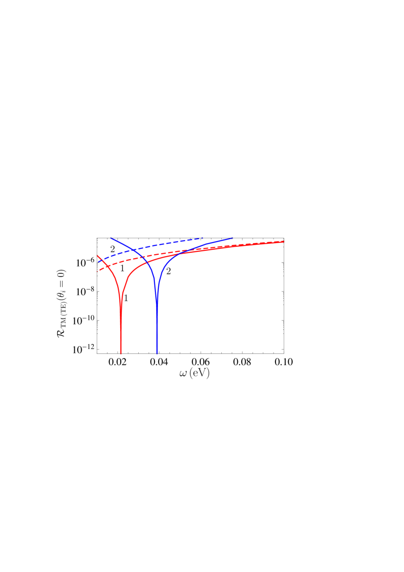
Figure 5: (Color online) The reflectivity of gapped graphene at $T=300\,$K at the normal incidence is shown in the vicinity of frequencies where it drops to zero by the solid lines 1 and 2 as a function of frequency for the mass-gap parameters $m=0.1$ and 0.05 eV, respectively. The dashed lines 1 and 2 reproduce the respective results at $T=0\,$K.

Now we perform numerical computations of the reflectivity of graphene at the normal incidence ($\theta_{i}=0$) defined via the reflection coefficients by the first equalities in Eq. (31). Computations are performed using Eqs. (5)–(7), (14)–(19), (23) and (25). As noted in Sec. IIIB, under the conditions $\tilde{v}_{F}\ll 1$, $\eta\approx 1$ the angular dependences of reflectivities are similar to the case of gapless graphene. They are presented in the above analytic expressions and in Figs. 3 and 5 of Ref. 38 . Taking into account the possibility of comparison with the measurement data, we consider the temperature at a laboratory, $T=300\,$K, and cover the maximally wide range of frequencies.

In Fig. 4 we present the computational results for the reflectivities ${\cal R}_{\rm TM}={\cal R}_{\rm TE}$ as functions of frequency by the two solid lines 1 and 2 for graphene sheets with the mass-gap parameter $m$ equal to 0.1 and 0.05 eV, respectively. The double logarithmic scale is used. The dashed lines 1 and 2 reproduce from Fig. 1 the respective results at zero temperature. As is seen in Fig. 4, the reflectivity of graphene depends heavily on the fact that temperature is not equal to zero.

First of all note that the reflectivity at zero frequency is equal to unity rather than zero, as it was at zero temperature (see Figs. 1 and 3). This fact was already established analytically in the asymptotic expressions (59), (62) and (66) valid at small frequencies.

Second, as was noted above, in the region of sufficiently small frequencies the thermal correction $\Delta\Pi_{00}$ in Eq. (65) is real and negative. Taking into account that at small frequencies $\Pi_{00}^{(0)}$ is real and positive [see Eqs. (6) and (30)], it is possible that $\Pi_{00}$ turns into zero at some frequency $\omega_{0}$ depending on $m$ and $T$. As is noted above, the reflection coefficients and reflectivities also vanish at the frequency $\omega_{0}$. From Fig. 4 it is seen that ${\cal R}_{\rm TM\,(TE)}(\omega_{0},\theta_{i})=0$ at $\omega_{0}\approx 0.02159$ and 0.03033 eV for graphene sheets with $m=0.1$ and $0.05\,$eV, respectively. An approximate analytic expression for $\omega_{0}$ is obtained in Eq. (67). As discussed above, at room temperature it can be applied only for the largest value $m=0.1\,$eV and even in this case it is slightly outside the validity region of the approximation used. However, comparing the numerical (0.02159 eV) and analytic (0.0234 eV) results for $\omega_{0}$, one can conclude that the approximate expression (67) leads to only 8.4% error.

In the region of higher frequencies satisfying Eq. (24) for the mass-gap parameters considered in Fig. 4 the computational results are similar to those obtained at $T=0\,$K. Here, we observe the resonance peaks at the border frequencies and the asymptotic regime at high frequencies, which does not depend on $\omega$. In this region the dashed line 1 coincides with the solid line 1 ($m=0.1\,$eV), and the dashed line 2 ($m=0.05\,$eV) only minor deviates from the solid line 2. One can conclude that in the range of low frequencies satisfying the condition (22) the reflectivity properties of gapped graphene at zero and room temperature are quite different. Now we perform numerical computations in order to investigate these differences in more details.

In Fig. 5, we present the reflectivity of graphene with $m=0.1$ and 0.05 eV at $T=300\,$K at the normal incidence in an immediate vicinity of the frequency $\omega_{0}$ where it drops to zero (the lines 1 and 2, respectively). For this purpose the natural scale is used along the frequency axis. The dashed lines 1 and 2 show the respective results at $T=0\,$K. As is seen in Fig. 5, near the frequencies $\omega_{0}$ it should be possible to observe the change in the reflectivity of graphene by several orders of magnitude.

From Fig. 4 it can be seen that with decreasing $m$ the interval between the frequency $\omega_{0}$, where the reflectivity vanishes, and the border frequency $2mc^{2}/\hbar$, where it is equal to unity, becomes more narrow. To illustrate this tendency, in Fig. 6 we plot the reflectivity of graphene with $m=0.001\,$eV at $T=300\,$K as a function of frequency in the double logarithmic scale (the solid line). From Fig. 6 it is seen that zero reflectivity is achieved at the frequency $\omega_{0}$ which is only slightly less than 0.002 eV. Because of this, the minimum and maximum values of the reflectivity virtually coincide. For not too high frequencies satisfying the condition $\hbar\omega\ll k_{B}T$ and with exception of some vicinity of the border frequency $2mc^{2}/\hbar$, the solid line in Fig. 6 is in a good agreement with the asymptotic expressions (59) and (61) taken at $\theta_{i}=0$.

In the same figure the reflectivity of graphene with $m=0.001\,$eV at zero temperature is shown by the dashed line. In this case the reflectivity has only the maximum value at 0.002 eV and goes to zero with vanishing frequency. Note that all the above results related to the region of frequencies (22) are valid only for graphene with nonzero mass-gap parameter. Specifically, the reflectivity of gapless graphene does not vanish at any frequency 38 .

Finally, we perform numerical computations of the frequency $\omega_{0}$, where the reflectivity of graphene vanishes, as a function of the mass-gap parameter $m$. The computational results in the region of $m$ from 0.001 to 0.1 eV at $T=300\,$K are shown in Fig. 7 by the solid line. As is seen in Fig. 7, with increasing $m$, the frequency $\omega_{0}$ increases, achieves the maximum value at $m\approx 0.03\,$eV and then gradually decreases. In the same figure, the border frequency $\omega=2mc^{2}/\hbar$ is plotted by the dashed line. It is seen that the frequency interval between the dashed and solid lines becomes narrower with decreasing $m$ (as already was concluded from Fig. 4 basing on only two values of $m$). The dashed line remains above the solid line at all $m$ and almost coincides with it at $m\lesssim 0.015\,$eV. This is in accordance with Fig. 6, where for $m=0.001\,$eV the frequencies, where reflectivity of graphene takes the minimum and maximum values, cannot be discerned.

V Conclusions and discussion

In the foregoing, we have investigated the reflectivity properties of gapped graphene at both zero and nonzero temperature in the framework of the Dirac model. It was shown that the presence of nonzero mass-gap parameter has a profound effect on the reflectivity of graphene. To find this effect, we have employed the polarization tensor of graphene found in Ref. 38 , which was further adapted and simplified for the case of gapped graphene. Specifically, it was shown that at zero temperature the reflectivities of gapped graphene go to zero when the frequency vanishes. This is not the case for a gapless graphene, where the reflectivities at zero temperature are nonzero and depend only on the fine structure constant and the angle of incidence. We have shown also that at nonzero temperature the reflectivities of gapped graphene go to unity with vanishing frequency, as it is for a gapless graphene.

Another distinctive property of gapped graphene is that its reflectivities possess the narrow resonances having the maximum values equal to unity at the border frequency $\omega=2mc^{2}/[\hbar\eta(\theta_{i})]$. This is the case at both zero and nonzero temperature and can be observed experimentally as a jump in the reflectivities of graphene when passing across the border frequency. At frequencies larger than the border frequency there is only minor influence of the mass-gap parameter on the reflectivities of graphene.

The next remarkable property of gapped graphene at nonzero temperature is that in the vicinity of some frequency $\omega_{0}$ smaller than the border frequency its reflectivities drop to zero. This local minimum also can be observed as a jump in the reflectivities of graphene when passing across the frequency $\omega_{0}$. There is no such effect for a gapless graphene or for a gapped graphene at $T=0\,$K. It is caused by the fact that the thermal correction to the polarization tensor takes negative values.

All the above effects have been derived and investigated analytically in different frequency regions. As a result, the approximate analytic expressions for the reflectivities of graphene and for the frequency $\omega_{0}$ have been found. Both the cases of the normal incidence and an arbitrary incidence angle were considered. The analytic results have been illustrated by numerical computations over a wide range of frequencies from $1\,\mu$eV to 20 eV. From the comparison between approximate analytic and computational results, the exactness of the former was estimated.

The developed theory of the reflectivity of gapped graphene at any temperature is based on the first principles of quantum electrodynamics. It can be used in many prospective applications of graphene, such as optical detectors, optoelectronic switches and other mentioned in Sec. I. In future it would be interesting to generalize this theory for the case of nonzero chemical potential (see Ref. 48 for the polarization tensor of graphene taking the chemical potential into account) and to apply it to graphene-coated substrates.

                      

                      

                      

                      

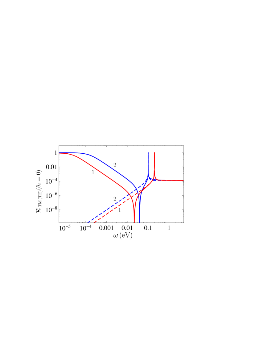
Figure 4: (Color online) The reflectivity of gapped graphene at $T=300\,$K at the normal incidence is shown by the solid lines 1 and 2 as a function of frequency for the mass-gap parameters $m=0.1$ and 0.05 eV, respectively. The dashed lines 1 and 2 reproduce the respective results at $T=0\,$K.

                      

                      

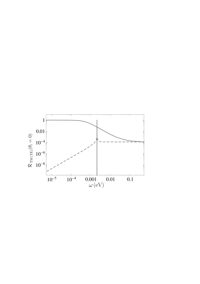
Figure 6: The reflectivity of gapped graphene with $m=0.001$ eV at the normal incidence is shown as a function of frequency by the solid and dashed lines at $T=300\,$K and $T=0\,$K, respectively.

                      

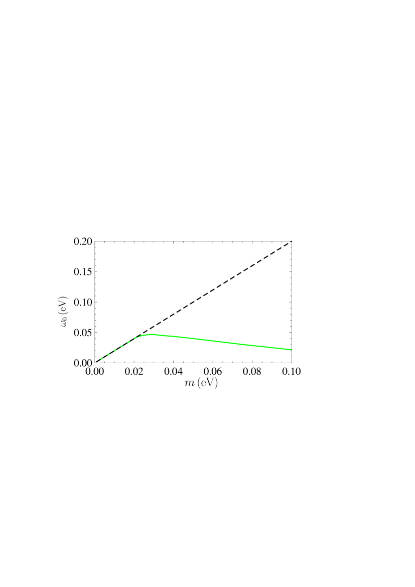
Figure 7: (Color online) The frequency, where the reflectivity of graphene at $T=300\,$K at the normal incidence vanishes, is shown by the solid line as a function of the mass-gap parameter. The dashed line shows the border frequency $2mc^{2}/\hbar$.

References

- (1) A. H. Castro Neto, F. Guinea, N. M. R. Peres, K. S. Novoselov, and A. K. Geim, Rev. Mod. Phys. 81, 109 (2009).
- (2) M. I. Katsnelson, Graphene: Carbon in two Dimensions (Cambridge University Press, Cambridge, 2012).
- (3) G. Gómez-Santos, Phys. Rev. B 80, 245424 (2009).
- (4) M. I. Katsnelson, K. S. Novoselov, and A. K. Geim, Nat. Phys. 2, 620 (2006).
- (5) D. Allor, T. D. Cohen, and D. A. McGady, Phys. Rev. D 78, 096009 (2008).
- (6) C. G. Beneventano, P. Giacconi, E. M. Santangelo, and R. Soldati, J. Phys A: Math. Theor. 42, 275401 (2009).
- (7) G. L. Klimchitskaya and V. M. Mostepanenko, Phys. Rev. D 87, 215011 (2013).
- (8) X. Jiang, Y. Cao, K. Wang, J. Wei, D. Wu, and H. Zhu, Surf. Coatings Technology 261, 327 (2015).
- (9) Springer Handbook of Nanomaterials, edited by R. Vajtai (Springer, Berlin, 2013).
- (10) S. Watcharotone, D. A. Dikin, S. Stankovich et al., Nano Lett. 7, 1888 (2007).
- (11) L. F. Dumée, L. He, Z. Wang et al., Carbon 87, 395 (2015).
- (12) T. Kuila, S. Bose, P. Khanra, A. K. Mishra, N. H. Kim, and J. H. Lee, Biosens. Bioelectr. 29, 4637 (2011).
- (13) Yu. V. Bludov, M. I. Vasilevskiy, and N. M. R. Peres, Europhys. Lett. 92, 68001 (2011).
- (14) R. R. Nair, P. Blake, A. N. Grigorenko, K. S. Novoselov, T. J. Booth, T. Stauber, N. M. R. Peres, and A. K. Geim, Science 320, 1308 (2008).
- (15) A. B. Kuzmenko, E. van Neumen, F. Carbone, and D. van der Marel, Phys. Rev. Lett. 100, 117401 (2008).
- (16) V. P. Gusynin, S. G. Sharapov, and J. P. Carbotte, Phys. Rev. Lett. 96, 256802 (2006).
- (17) V. P. Gusynin, S. G. Sharapov, and J. P. Carbotte, Int. J. Mod. Phys. B 21, 4611 (2007).
- (18) L. A. Falkovsky and S. S. Pershoguba, Phys. Rev. B 76, 153410 (2007).
- (19) T. Stauber, N. M. R. Peres, and A. K. Geim, Phys. Rev. B 78, 085432 (2008).
- (20) F. H. L. Koppens, D. E. Chang, and F. J. García de Abajo, Nano Lett. 11, 3370 (2011).
- (21) M. Bordag, I. V. Fialkovsky, D. M. Gitman, and D. V. Vassilevich, Phys. Rev. B 80, 245406 (2009).
- (22) I. V. Fialkovsky, V. N. Marachevsky, and D. V. Vassilevich, Phys. Rev. B 84, 035446 (2011).
- (23) M. Bordag, G. L. Klimchitskaya, and V. M. Mostepanenko, Phys. Rev. B 86, 165429 (2012).
- (24) M. Chaichian, G. L. Klimchitskaya, V. M. Mostepanenko, and A. Tureanu, Phys. Rev. A 86, 012515 (2012).
- (25) G. L. Klimchitskaya and V. M. Mostepanenko, Phys. Rev. B 87, 075439 (2013).
- (26) G. L. Klimchitskaya, V. M. Mostepanenko, and Bo E. Sernelius, Phys. Rev. B 89, 125407 (2014).
- (27) G. L. Klimchitskaya, U. Mohideen, and V. M. Mostepanenko, Phys. Rev B 89, 115419 (2014).
- (28) G. L. Klimchitskaya and V. M. Mostepanenko, Phys. Rev A 89, 052512 (2014).
- (29) G. L. Klimchitskaya and V. M. Mostepanenko, Phys. Rev. B 91, 045412 (2015).
- (30) G. L. Klimchitskaya and V. M. Mostepanenko, Phys. Rev B 91, 174501 (2015).
- (31) D. Drosdoff and L. M. Woods, Phys. Rev. B 82, 155459 (2010).
- (32) D. Drosdoff and L. M. Woods, Phys. Rev. A 84, 062501 (2011).
- (33) Bo E. Sernelius, Europhys. Lett. 95, 57003 (2011).
- (34) Bo E. Sernelius, Phys. Rev. B 85, 195427 (2012).
- (35) A. D. Phan, L. M. Woods, D. Drosdoff, I. V. Bondarev, and N. A. Viet, Appl. Phys. Lett. 101, 113118 (2012).
- (36) M. Bordag, G. L. Klimchitskaya, U. Mohideen, and V. M. Mostepanenko, Advances in the Casimir Effect (Oxford University Press, Oxford, 2015).
- (37) G. L. Klimchitskaya, U. Mohideen, and V. M. Mostepanenko, Rev. Mod. Phys. 81, 1827 (2009).
- (38) M. Bordag, G. L. Klimchitskaya, V. M. Mostepanenko, and V. M. Petrov, Phys. Rev. D 91, 045037 (2015); Phys. Rev. D93, 089907(E) (2016).
- (39) G. L. Klimchitskaya, C. C. Korikov, and V. M. Petrov, Phys. Rev. B 92, 125419 (2015); Phys. Rev. B 93, 159906(E) (2016).
- (40) S. A. Jafari, J. Phys.: Condens. Matter 24, 205802 (2012).
- (41) P. K. Pyatkovsky, J. Phys.: Condens. Matter 21, 025506 (2009).
- (42) V. P. Gusynin, S. G. Sharapov, and J. P. Carbotte, New J. Phys. 11, 095013 (2009).
- (43) V. P. Gusynin and S. G. Sharapov, Phys. Rev. B 73, 245411 (2006).
- (44) A. I. Akhiezer and V. B. Berestetskii, Quantum Electrodynamics (Interscience, New York, 1965).
- (45) S. S. Schweber, An Introduction to Relativistic Quantum Field Theory (Dover, New York, 2005).
- (46) M. I. Katsnelson, Eur. Phys. J. B 51, 157 (2006).
- (47) I. S. Gradshtein and I. M. Ryzhik, Table of Integrals, Series and Products (Academic Press, New York, 1980).
- (48) M. Bordag, I. Fialkovsky, and D. Vassilevich, Phys. Rev. B 93, 075414 (2016).