Satisfiability-Based Methods for Reactive Synthesis from Safety Specifications

Abstract

Existing approaches to synthesize reactive systems from declarative specifications mostly rely on Binary Decision Diagrams (BDDs), inheriting their scalability issues. We present novel algorithms for safety specifications that use decision procedures for propositional formulas (SAT solvers), Quantified Boolean Formulas (QBF solvers), or Effectively Propositional Logic (EPR). Our algorithms are based on query learning, templates, reduction to EPR, QBF certification, and interpolation. A parallelization combines multiple algorithms. Our optimizations expand quantifiers and utilize unreachable states and variable independencies. Our approach outperforms a simple BDD-based tool and is competitive with a highly optimized one. It won two medals in the SyntComp competition.

1 Introduction

A common criticism of formal verification techniques such as model checking [1, 2] is that they are only applied after the implementation is completed. Synthesis [3] is more ambitious: it constructs an implementation from a declarative specification automatically. The specification may only express what the system shall do, but not how. Hence, writing a specification can be significantly easier than implementing it. Another advantage is that synthesized implementations are correct-by-construction, i.e., guaranteed to satisfy the specification from which they have been constructed. Assuming that the specification expresses the design intent correctly and completely, this eliminates the need for verification and debugging of the implementation. This effort reduction is illustrated in Figure 1.

Applications of synthesis. Synthesis is particularly well suited for rapid prototyping, where a working implementation needs to be available quickly. A synthesized prototype can later be exchanged by a (manual) implementation that is more optimized. Another interesting application is program sketching [4, 5], where the programmer can leave “holes” in the code. A synthesizing compiler then fills the holes such that a given specification is satisfied. This mix of imperative and declarative programming is appealing because some aspects of the program may be easy to implement, while others may be easier to specify. In controller synthesis, a plant needs to be controlled such that some specification is satisfied. Synthesizing such a controller is similar to program sketching in that a given part (the plant) is combined with a synthesized part (the controller). Another related application is automatic program repair [6, 7], where potentially faulty program parts (identified by some error localization algorithm) are replaced by synthesized corrections. In all these applications, automatic synthesis contributes to keeping the manual development effort low.

Systems. This article is concerned with synthesis algorithms for reactive systems [8], which interact with their environment in a synchronous way: in every time step, the environment provides input values and the system responds with output values. This is repeated ad infinitum, i.e., reactive systems conceptually never terminate. Thus, reactive systems can directly model (synchronous) hardware designs, but also other non-terminating systems such as an operating system, a server implementing some protocol, etc. In contrast, transformational systems terminate after processing their input. They are thus suited to model procedures of a software program, e.g., a sorting algorithm.

Specifications. We focus on synthesis of reactive systems from safety specifications, which express that certain “bad things” never happen. This stands in contrast to liveness properties, which stipulate that certain “good things” must happen eventually. Synthesis algorithms for safety specifications can be useful even for specifications that contain liveness properties. First, bounded synthesis approaches [9, 10] can reduce synthesis from richer specifications, such as Linear Temporal Logic (LTL) [11], to safety synthesis problems by setting a bound on the reaction time. For instance, instead of requiring that some event happens eventually, one may require that it happens within at most $k$ steps. Clearly, a realization of the latter is also a realization of the former. By choosing $k$ as low as possible (such that a solution still exists), we may even get systems that react faster. A second reason why safety specifications are important is that safety properties often make up the bulk of a specification and they can be handled in a compositional manner: the safety synthesis problem can be solved before the other properties are handled [12].

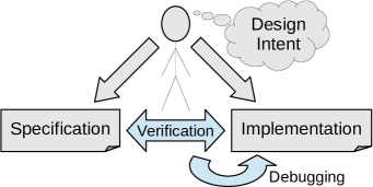
(a)

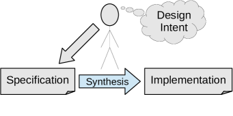
(b)

Figure 1: Reduction of the development effort due to synthesis

Synthesis is a game. Model checking can be understood as (exhaustive) search for inputs under which a (model of the) system violates its specification. That is, the inputs are the only source of non-determinism. Synthesis, on the other hand, needs to handle two sources of non-determinism: the unknown inputs and the (yet) unknown system implementation. Synthesis can thus be seen as a game between two players: The environment player controls the inputs of

the system to be synthesized. The system player controls the outputs and attempts to satisfy the specification for every environment behavior. The environment player has the role of the antagonist, trying to violate the specification. The game-based approach to synthesis computes a strategy for the system player to win the game (i.e., to satisfy the specification) against every environment player. An implementation of such a winning strategy forms the solution. Computing a winning strategy involves dealing with alternating quantifiers because for every input (or environment behavior) there must exist some output (or system behavior) satisfying the specification. This stands in contrast to model checking, where existential quantification suffices.

Scalability. Synthesis is computationally hard. For safety specifications, the worst-case time complexity is exponential [13, 14] in the size of the specification. For LTL, it is even doubly exponential [15]. Measures to improve the performance in practice include limiting the expressiveness of the specification [16, 17], limiting the size of systems to construct [18], and applying symbolic algorithms [19], which use formulas as a compact representation of state sets instead of enumerating states explicitly. These formulas can in turn be represented using Binary Decision Diagrams (BDDs) [20], a graph-based representation for propositional formulas. However, for certain structures, BDDs are known to explode in size and thus scale insufficiently [20]. This is one reason why BDDs have largely been displaced by SAT solvers in model checking. Yet, in reactive synthesis, BDDs are still the predominant symbolic reasoning engine. This is witnessed by the fact that all submissions to the reactive synthesis competition SyntComp in 2014 [21] and 2015 [22], except for our own, were BDD-based. One reason is that synthesis inherently deals with alternating quantifiers (see above). BDDs provide universal and existential quantifier elimination to deal with that.

Contributions and Outline

To offer additional alternatives to BDDs in reactive synthesis, we present novel synthesis algorithms for safety specifications using decision procedures for the satisfiability of propositional formulas (SAT solvers), Quantified Boolean Formulas (QBF solvers), or Effectively Propositional Logic (EPR), which is a subset of first-order logic. Our algorithms exploit solver features such as incremental solving and unsatisfiable cores by design. Similar to existing solutions, our approach consists of two steps: computing a strategy and building a circuit that implements this strategy.

Preliminaries. Before we present our algorithms, Chapter 2 introduces background and notation. It starts by defining logics and decision procedures. Readers who are familiar with SAT and QBF can focus on Section 2.2.2.1 and 2.2.3.1 to understand our notation. In Section 2.4, we define the addressed synthesis problem and give a textbook solution. Synthesis experts can focus on Definition 4. Finally, we introduce query learning [23] and Counterexample-Guided Inductive Synthesis (CEGIS) [4] as algorithmic principles underlying many of our algorithms.

Strategy computation. Chapter 3 presents our algorithms and optimizations for computing a strategy to satisfy the specification. Section 3.1 starts with a learning algorithm that uses a QBF solver. In Section 3.2, we modify this algorithm to use a plain SAT solver while exploiting incremental solving and unsatisfiable cores. This turns out to be significantly faster. Both these sections contain correctness proofs and discuss possible variations and an efficient implementation. In Section 3.3, we reduce the number of iterations (and thereby the execution time) of the SAT solver based solution by partially expanding quantifiers. Section 3.4 continues with optimizations that exploit unreachable states based on concepts from the model checking algorithm IC3 [24]. Both optimizations give a speedup of more than one order of magnitude each. In Section 3.5, we describe a completely different approach, which fixes the structure of the solution using a template. We compute solutions either with a single call to a QBF solver or by calling a SAT solver repeatedly using (an extension of) CEGIS [4]. Section 3.6 is similar in spirit but avoids the template by formulating the problem in EPR. Since different algorithms perform well in different cases, we finally present a parallelization that combines various methods and configurations in multiple threads while exchanging fine-grained information.

Circuit computation. Chapter 4 is devoted to computing an implementation in the form of a circuit from a given strategy. The goal is to obtain small circuits efficiently. To this end, implementation freedom available in the strategy needs to be exploited wisely. We present a number of satisfiability-based methods that not only work for safety specifications but also for strategies to satisfy other objectives. For each method, we thus present the general solution as well as an efficient realization for the special case of safety synthesis problems. We start with an approach based on QBF certification [25] in Section 4.1. In Section 4.2, we use a QBF solver in a learning algorithm. This performs better, especially when using incremental QBF solving. Section 4.3 adopts the interpolation-based approach by Jiang et al. [26] and extends it with an optimization to exploit variable (in)dependencies. In Section 4.4, we combine the approach by Jiang et al. [26] with query learning as a special interpolation procedure. This improves the speed and the resulting circuit size by around two orders of magnitude. Finally, we present a parallelization that combines multiple methods in different threads with the aim to inherit their strengths and to compensate their weaknesses.

Tool. We implemented our methods in an open-source tool named Demiurge. It supports the input format of the reactive synthesis competition SyntComp [21] and won two medals in this competition. Demiurge is extendable and highly configurable regarding solvers, methods and optimizations to use. We describe Demiurge in Section 5.1.

Experiments. In Chapter 5, we evaluate our approach on the SyntComp benchmarks. We compare our different methods and evaluate the effect of optimizations. We also investigate the performance of different methods on different classes of benchmarks. Our parallelization turns out to be faster than a BDD-based tool by one order of magnitude and produces circuits that are smaller by two orders of magnitude. Our tool is even competitive with AbsSynthe [13], a BDD-based tool that implements advanced concepts such as abstraction/refinement.

Conclusion. Since our approach is particularly superior for certain benchmark classes, we conclude that it forms a valuable complement to existing approaches. Moreover, decision procedures for satisfiability are an active field of research, and enormous scalability improvements are witnessed by various competitions over the years. Since our algorithms use such decision procedures as a black box, they directly benefit from future developments in this field.

Relation to previous work. This is the manuscript of an article that has been submitted to the Journal of Computer and System Sciences (JCSS). It is based on earlier work by the authors [27, 28], which has been extended with additional optimizations and variations of algorithms, as well as a more elaborate experimental evaluation. This entire work forms the basis of a dissertation [29].

2 Preliminaries and Notation

We will use upper case letters for sets, lower case letters for set elements, and calligraphic fonts for tuples defining more complex structures. We denote the Boolean domain by $\mathbb{B}=\{\mathsf{true},\mathsf{false}\}$ and write iff for “if and only if”.

2.1 Logics

We will use various kinds of logics to solve synthesis problems. This section introduces these logics. Decision procedures and reasoning engines for these logics will then be introduced in Section 2.2.

Variables and formulas. We will use lower case letters for variables and capital letters to denote formulas. Recall that capital letters are also used to denote sets, but this is no coincidence since we will later use formulas to represent sets (see Section 2.3). Vectors of variables will be written with an overline. For clarity, we will often write the variables that occur freely in a formula in brackets. For instance, $F(\overline{x})$ denotes a formula over the variables $\overline{x}=(x_{1},x_{2},\ldots,x_{n})$. If the variables are clear from the context, we will sometimes omit the brackets, i.e., write only $F$ instead of $F(\overline{x})$. Furthermore, we will use the brackets to denote variable substitutions: if $F(\ldots,x,\ldots)$ is a formula, we denote by $F(\ldots,y,\ldots)$ the same formula but with all occurrences of $x$ replaced by $y$. With a slight abuse of notation, we will also treat vectors of variables like sets if the order of the elements is irrelevant. For instance, $\overline{x}\cup\overline{y}$ denotes a concatenation of two variable vectors, and $\overline{x}\setminus\{x_{i}\}$ denotes the variable vector $\overline{x}$ but with element $x_{i}$ removed.

Operator precedence. Save for cases where too many brackets hamper readability, we will avoid ambiguities in operator precedence. However, for the avoidance of doubt, will will use the following precedence order (from stronger to weaker binding) for operators in formulas: $\neg,\wedge,\vee,\rightarrow,\leftrightarrow,\forall,\exists$.

2.1.1 Propositional Logic

All variables in propositional logic are Boolean, i.e., take values from $\mathbb{B}=\{\mathsf{true},\mathsf{false}\}$. We will use the Boolean connectives $\neg$, $\wedge$, $\vee$, $\rightarrow$, $\leftrightarrow$, encoding negation, conjunction, disjunction, implication, and equivalence, respectively.

Conjunctive Normal Forms (CNFs). A literal is a Boolean variable or its negation. A clause is a disjunction of literals. A cube is a conjunction of literals. We will sometimes treat clauses and cubes as sets of literals. For instance, given that $l$ is a literal and $c_{1},c_{2}$ are clauses, we write $l\in c_{1}$ to denote that $l$ occurs as a disjunct in clause $c_{1}$, and we write $c_{1}\subseteq c_{2}$ to denote that all literals of clause $c_{1}$ also occur in clause $c_{2}$. A propositional formula is in Conjunctive Normal Form (CNF) if it is written as a conjunction of clauses. There are two reasons why CNF representations are important. First, decision procedures for satisfiability usually require the input formula to be in CNF. Second, every formula can be transformed into an equisatisfiable formula in CNF by introducing at most a linear amount of auxiliary variables. This is called Tseitin transformation [30]. An improvement by exploiting the polarity (even or odd number of negations) of subformulas to obtain smaller CNF encodings has been proposed by Plaisted and Greenbaum [31].

Variable assignments. We use cubes to describe (potentially partial) truth assignments to variables: unnegated variables of the cube are set to $\mathsf{true}$, negated ones are $\mathsf{false}$. We use bold letters to denote cubes. For instance, $\mathbf{x}$ denotes a cube over the variables $\overline{x}$. An $\overline{x}$-minterm is a cube that contains all variables of $\overline{x}$ either negated or unnegated (but not both). Thus, minterms describe complete assignments to Boolean variables. We write $\mathbf{x}\models F(\overline{x})$ to denote that the $\overline{x}$-minterm $\mathbf{x}$ satisfies the formula $F(\overline{x})$. Given a formula $F(\ldots,\overline{x},\ldots)$ and an $\overline{x}$-minterm $\mathbf{x}$, we write $F(\ldots,\mathbf{x},\ldots)$ to denote the formula $F$ but with all occurrences of the variables $\overline{x}$ replaced by their respective truth value defined by $\mathbf{x}$.

Unsatisfiable cores. Let $F$ be an unsatisfiable formula in CNF. A clause-level unsatisfiable core is a subset of the clauses of $F$ that is still unsatisfiable. While this definition is widely used, many applications require the minimization of “interesting” constraints while the remaining constraints remain fixed. For such problems, Nadel [32] coined the term high-level unsatisfiable core. To support such high-level unsatisfiable cores, we use the following definition. Let $\mathbf{x}$ be a cube and let $F(\overline{x},\overline{y})$ be a formula such that $\mathbf{x}\wedge F$ is unsatisfiable. An unsatisfiable core of $\mathbf{x}$ with respect to $F$ is a subset $\mathbf{x}^{\prime}\subseteq\mathbf{x}$ of the literals in $\mathbf{x}$ such that $\mathbf{x}^{\prime}\wedge F$ is still unsatisfiable. An unsatisfiable core $\mathbf{x}^{\prime}$ is minimal if no proper subset $\mathbf{x}^{\prime\prime}$ of $\mathbf{x}^{\prime}$ makes $\mathbf{x}^{\prime\prime}\wedge F$ unsatisfiable. With this definition, high-level unsatisfiable cores can be computed by adding conjuncts of the form $x_{i}\rightarrow G(\overline{y})$ for $x_{i}\in\overline{x}$ to $F(\overline{x},\overline{y})$. This way, the constraint $G(\overline{y})$ can be enabled or disabled via the truth value of $x_{i}$. Moreover, this notion of unsatisfiable cores is directly supported by many solver.

Interpolants. Let $A(\overline{x},\overline{y})$ and $B(\overline{x},\overline{z})$ be two propositional formulas such that $A\wedge B$ is unsatisfiable, and $\overline{y}$ and $\overline{z}$ are disjoint. A Craig interpolant [33] is a formula $I(\overline{x})$ such that $A\rightarrow I\rightarrow\neg B$. Intuitively, the interpolant is a formula that is weaker than $A$, but still strong enough to make $I\wedge B$ unsatisfiable. In addition to that, the interpolant references only the variables $\overline{x}$ that occur both in $A$ and in $B$.

Cofactors. Let $F(\ldots,x,\ldots)$ be a propositional formula. The positive cofactor of $F$ regarding $x$ is the formula $F(\ldots,\mathsf{true},\ldots)$, where all occurrences of $x$ have been replaced by $\mathsf{true}$. Analogously, the negative cofactor of $F$ regarding $x$ is the formula $F(\ldots,\mathsf{false},\ldots)$.

2.1.2 Quantified Boolean Formulas

Quantified Boolean Formulas (QBFs) [34] extend propositional logic with universal (denoted $\forall$) and existential (denoted $\exists$) quantification of variables. The quantifiers have their expected semantics: Since propositional variables can only be either $\mathsf{true}$ or $\mathsf{false}$, $\exists x_{i}\operatorname{\mathbin{:}}F(\ldots,x_{i},\ldots)$ can be seen as a shorthand for $F(\ldots,\mathsf{true},\ldots)\vee F(\ldots,\mathsf{false},\ldots)$. Likewise, $\forall x_{i}\operatorname{\mathbin{:}}F(\ldots,x_{i},\ldots)$ is short for $F(\ldots,\mathsf{true},\ldots)\wedge F(\ldots,\mathsf{false},\ldots)$. Using these rules, a Quantified Boolean Formula (QBF) can always be transformed into a purely propositional formula. However, this usually causes a significant blow-up in formula size.

PCNFs. A QBF is in Prenex Conjunctive Normal Form (PCNF) if it is written in the form

$$Q_{1}\overline{x}_{1}\operatorname{\mathbin{:}}Q_{2}\overline{x}_{2}\operatorname{\mathbin{:}}\ldots Q_{k}\overline{x}_{k}\operatorname{\mathbin{:}}F(\overline{x}_{1},\overline{x}_{2},\ldots,\overline{x}_{k}),$$

where $Q_{i}\in\{\forall,\exists\}$ and $F$ is a propositional formula in CNF. In this formulation, we use $Q_{i}\overline{x}_{i}$ as a shorthand for $Q_{i}x_{i,1}\operatorname{\mathbin{:}}\ldots Q_{i}x_{i,n}$ with $\overline{x}_{i}=(x_{i,1},\ldots,x_{i,n})$. We refer to $Q_{1}\overline{x}_{1}\operatorname{\mathbin{:}}Q_{2}\overline{x}_{2}\operatorname{\mathbin{:}}\ldots Q_{k}\overline{x}_{k}$ as the quantifier prefix and call $F(\overline{x}_{1},\overline{x}_{2},\ldots,\overline{x}_{k})$ the matrix of the PCNF. We require every PCNF to be closed in the sense that all variables occurring in the matrix must be quantified either existentially or universally. Hence, a QBF in PCNF can only be valid (equivalent to $\mathsf{true}$) or unsatisfiable (equivalent to $\mathsf{false}$).

Skolem functions. Let $\exists\overline{a}_{1}\operatorname{\mathbin{:}}\forall\overline{b}_{1}\operatorname{\mathbin{:}}\ldots\exists\overline{a}_{k}\operatorname{\mathbin{:}}\forall\overline{b}_{k}\operatorname{\mathbin{:}}\exists\overline{c}\operatorname{\mathbin{:}}Q_{1}\overline{d}_{1}\operatorname{\mathbin{:}}\ldots Q_{l}\overline{d}_{l}\operatorname{\mathbin{:}}F(\overline{a}_{1},\overline{b}_{1},\ldots,\overline{a}_{k},\overline{b}_{k},\overline{c},\overline{d}_{1},\ldots,\overline{d}_{l})$ with $Q_{i}\in\{\forall,\exists\}$ be a QBF in PCNF that is valid. A Skolem function for the existentially quantified variables $\overline{c}$ is a function $f:2^{|\overline{b}_{1}|}\times\ldots\times 2^{|\overline{b}_{k}|}\rightarrow 2^{|\overline{c}|}$ that defines the values of the variables $\overline{c}$ based on the universally quantified variables $\overline{b}_{1},\ldots,\overline{b}_{k}$ occurring before $\overline{c}$ in the quantifier prefix such that

$$\exists\overline{a}_{1}\operatorname{\mathbin{:}}\forall\overline{b}_{1}\operatorname{\mathbin{:}}\ldots\exists\overline{a}_{k}\operatorname{\mathbin{:}}\forall\overline{b}_{k}\operatorname{\mathbin{:}}Q_{1}\overline{d}_{1}\operatorname{\mathbin{:}}\ldots Q_{l}\overline{d}_{l}\operatorname{\mathbin{:}}F\bigl{(}\overline{a}_{1},\overline{b}_{1},\ldots,\overline{a}_{k},\overline{b}_{k},f(\overline{b}_{1},\ldots,\overline{b}_{k}),\overline{d}_{1},\ldots,\overline{d}_{l}\bigr{)}$$

is still valid. The function $f$ can be seen as a certificate to show that values for the variables $\overline{c}$ making the QBF $\mathsf{true}$ exist (for any values of the variables $\overline{b}_{1},\ldots,\overline{b}_{k}$). Note that $f$ cannot depend on the variables $\overline{d}_{1},\ldots,\overline{d}_{l}$ occurring after $\overline{c}$ in the quantifier prefix, independent of whether some $\overline{d}_{i}$ is quantified universally or existentially.

Herbrand functions. A Herbrand function is the dual of a Skolem function for a QBF that is unsatisfiable. Let $\exists\overline{a}_{1}\operatorname{\mathbin{:}}\forall\overline{b}_{1}\operatorname{\mathbin{:}}\ldots\exists\overline{a}_{k}\operatorname{\mathbin{:}}\forall\overline{b}_{k}\operatorname{\mathbin{:}}\forall\overline{c}\operatorname{\mathbin{:}}Q_{1}\overline{d}_{1}\operatorname{\mathbin{:}}\ldots Q_{l}\overline{d}_{l}\operatorname{\mathbin{:}}F(\overline{a}_{1},\overline{b}_{1},\ldots,\overline{a}_{k},\overline{b}_{k},\overline{c},\overline{d}_{1},\ldots,\overline{d}_{l})$ be an unsatisfiable QBF. A Herbrand function for the universally quantified variables $\overline{c}$ is a function $f:2^{|\overline{a}_{1}|}\times\ldots\times 2^{|\overline{a}_{k}|}\rightarrow 2^{|\overline{c}|}$ that defines the values of the variables $\overline{c}$ based on the existentially quantified variables $\overline{a}_{1},\ldots,\overline{a}_{k}$ occurring before $\overline{c}$ in the quantifier prefix such that $\exists\overline{a}_{1}\operatorname{\mathbin{:}}\forall\overline{b}_{1}\operatorname{\mathbin{:}}\ldots\exists\overline{a}_{k}\operatorname{\mathbin{:}}\forall\overline{b}_{k}\operatorname{\mathbin{:}}Q_{1}\overline{d}_{1}\operatorname{\mathbin{:}}\ldots Q_{l}\overline{d}_{l}\operatorname{\mathbin{:}}F\bigl{(}\overline{a}_{1},\overline{b}_{1},\ldots,\overline{a}_{k},\overline{b}_{k},f(\overline{b}_{1},\ldots,\overline{b}_{k}),\overline{d}_{1},\ldots,\overline{d}_{l}\bigr{)}$ is still unsatisfiable.

Universal expansion. Let $G=Q_{1}\overline{x}_{1}\operatorname{\mathbin{:}}\ldots Q_{k}\overline{x}_{k}\operatorname{\mathbin{:}}\forall y\operatorname{\mathbin{:}}\exists\overline{z}\operatorname{\mathbin{:}}F(\overline{x}_{1},\ldots,\overline{x}_{k},y,\overline{z})$ be a QBF in PCNF. The universal expansion [35] of variable $y$ in $G$ is the formula $G^{\prime}=Q_{1}\overline{x}_{1}\operatorname{\mathbin{:}}\ldots Q_{k}\overline{x}_{k}\operatorname{\mathbin{:}}\exists\overline{z},\overline{z}^{\prime}\operatorname{\mathbin{:}}F(\overline{x}_{1},\ldots,\overline{x}_{k},\mathsf{true},\overline{z})\wedge F(\overline{x}_{1},\ldots,\overline{x}_{k},\mathsf{false},\overline{z}^{\prime}),$ where $\overline{z}^{\prime}$ is a fresh copy of the variables $\overline{z}$. This transformation is equivalence preserving [35]. In our formulation, the universally quantified variable $y$ to expand must only be followed by existential quantifications in the prefix. The variables $\overline{z}$ may depend on $y$ in $G$, i.e., may take different values for different truth values of $y$. Hence, they need to be renamed in one copy of the matrix when turning the universal quantification into a conjunction. Note that $G^{\prime}$ is in PCNF again because the conjunction of two CNFs is again a CNF.

One-point rule. Let $\mathbf{x}$ be an $\overline{x}$-minterm. We have that

$$\Bigl{(}\forall\overline{x}\operatorname{\mathbin{:}}\mathbf{x}\rightarrow F(\overline{x},\overline{y})\Bigr{)}\leftrightarrow\Bigl{(}F(\mathbf{x},\overline{y})\Bigr{)}\leftrightarrow\Bigl{(}\exists\overline{x}\operatorname{\mathbin{:}}\mathbf{x}\wedge F(\overline{x},\overline{y})\Bigr{)}$$ (1)

holds true because, in all three formulations, $F$ has to hold for a given $\overline{y}$-assignment if and only if the variables $\overline{x}$ have the specific truth values defined by $\mathbf{x}$. A slightly more complicated instance of this rule can be formulated as follows. Let $T(\overline{z},\overline{x})$ be a formula that defines the variables $\overline{x}$ uniquely based on the values of some other variables $\overline{z}$. Formally, we assume that $\forall\overline{z}\operatorname{\mathbin{:}}\exists\overline{x}\operatorname{\mathbin{:}}T(\overline{z},\overline{x})$ and $\forall\overline{z},\overline{x}_{1},\overline{x}_{2}\operatorname{\mathbin{:}}\bigl{(}T(\overline{z},\overline{x}_{1})\wedge T(\overline{z},\overline{x}_{2})\bigr{)}\rightarrow(\overline{x}_{1}=\overline{x}_{2})$. We have that

$$\Bigl{(}\forall\overline{x}\operatorname{\mathbin{:}}T(\overline{z},\overline{x})\rightarrow F(\overline{x},\overline{y})\Bigr{)}\leftrightarrow\Bigl{(}\exists\overline{x}\operatorname{\mathbin{:}}T(\overline{z},\overline{x})\wedge F(\overline{x},\overline{y})\Bigr{)}$$ (2)

holds true because for a given $\overline{z}$-assignment $\mathbf{z}$ and a given $\overline{y}$-assignment $\mathbf{y}$, $F$ needs to hold only for the $\overline{x}$-assignment $\mathbf{x}$ that is uniquely defined by $T$ in both formulations. We will use these dualities in various proofs and transformations.

2.1.3 First-Order Logic

First-Order Logic (FOL) [36] is a more expressive logic, which enables reasoning about elements from arbitrary domains. Let $\mathbb{D}$ be a (potentially infinite) domain and let $\overline{x}=(x_{1},x_{2},\ldots,x_{k})$ be variables ranging over this domain. Furthermore, let $\overline{y}=(y_{1},y_{2},\ldots,y_{l})$ be Boolean variables ranging over $\mathbb{B}$, let $f_{1},f_{2},\ldots,f_{m}$ be function symbols and let $p_{1},p_{2},\ldots,p_{n}$ be predicate symbols. Each function symbol and each predicate symbol has a certain arity, i.e., number of arguments to which it can be applied. A term in first-order logic is either a domain variable $x_{i}$ (with $1\leq i\leq k$) or a function application $f_{i}(t_{1},\ldots,t_{a})$, where $f_{i}$ is a function symbol with arity $a$, and all $t_{i}$ (with $1\leq i\leq a$) are terms. Intuitively, a term evaluates to an element of $\mathbb{D}$. An atom is either a propositional variable $y_{i}$ (with $1\leq i\leq l$) or a predicate application $p_{i}(t_{1},\ldots,t_{a})$ where $p_{i}$ is a predicate symbol with arity $a$, and all $t_{i}$ (with $1\leq i\leq a$) are terms. Thus, intuitively, an atom evaluates to a truth value from $\mathbb{B}$. Finally, a First-Order Logic (FOL) formula is one of

$$a,\quad\neg F_{1},\quad F_{1}\vee F_{2},\quad F_{1}\wedge F_{2},\quad F_{1}\rightarrow F_{2},\quad F_{1}\leftrightarrow F_{2},\quad\exists x_{i}\operatorname{\mathbin{:}}F_{1},\text{ or }\quad\forall x_{i}\operatorname{\mathbin{:}}F_{1},$$

where $F_{1}$ and $F_{2}$ are First-Order Logic formulas themselves and $a$ is an atom. The semantics of the Boolean connectives and the quantifiers are as expected. A model of a FOL formula is a structure that satisfies the formula. It consists of concrete values for all variables that are not explicitly quantified, as well as concrete realizations of all functions $f_{i}$ and predicates $p_{i}$. Similar to propositional logic, we refer to an atom or the negation of an atom as a first-order literal. A first-order clause is a disjunction of first-order literals. A first-order CNF is a conjunction of first-order clauses. A FOL formula is quantifier-free if it contains no occurrences of $\exists$ and $\forall$.

2.1.4 Effectively Propositional Logic

Effectively Propositional Logic (EPR) [37], also known as Bernays-Schönfinkel class, is a subset of first-order logic that contains formulas of the form $\exists\overline{x}\operatorname{\mathbin{:}}\forall\overline{y}\operatorname{\mathbin{:}}F$, where $\overline{x}$ and $\overline{y}$ are disjoint vectors of variables ranging over domain $\mathbb{D}$, and $F$ is a function-free first-order CNF. The formula $F$ can contain predicates over $\overline{x}$ and $\overline{y}$, though.

2.2 Decision Procedures and Reasoning Engines

In the following, we will discuss decision procedures and reasoning engines for the logics introduced in the previous section from a user’s perspective.

2.2.1 Binary Decision Diagrams

Binary Decision Diagrams (BDDs) [20] are a graph-based representation for formulas in propositional logic. The graphs are rooted and acyclic. There are two terminal nodes, which we denote by 0 and 1. Non-terminal nodes are labeled by a variable, have exactly two outgoing edges, and act as decisions: when traversing the graph from the root node, depending on the truth value of the variable labelling a node, one of the outgoing edges is taken. If the terminal node 0 is reached during such a traversal, then this means that the formula evaluates to $\mathsf{false}$ for this assignment. If 1 is reached, the formula evaluates to $\mathsf{true}$.

Example 1. A Binary Decision Diagram (BDD) for the formula $f=(x\vee y)\wedge\neg z$ is shown on the right. The root node, representing $f$, is marked with an incoming arrow. Non-terminal nodes are drawn as circles. The solid outgoing edge is taken if the variable written in the node is $\mathsf{true}$, the dashed edge is taken if the variable written in the node is $\mathsf{false}$. The two terminal nodes are drawn as boxes. The graph can be read as follows: If $z=\mathsf{true}$, the entire formula $f$ is $\mathsf{false}$. Otherwise, $x$ is considered. If $x$ is $\mathsf{true}$ (and $z=\mathsf{false}$), the formula is $\mathsf{true}$. Otherwise, $y$ is considered. If $y=\mathsf{true}$ (and $z=x=\mathsf{false}$), then $f$ is $\mathsf{true}$. If $y=\mathsf{false}$ (and $z=x=\mathsf{false}$), then $f$ is $\mathsf{false}$.

Orderdness and Reducedness. BDDs are ordered in the sense that for all paths from the root to the terminal nodes, decisions on the variables are always taken in the same order. We will refer to this order as the variable order of the BDD. For instance, the variable order in Example 2.2.1 is $z,x,y$. Furthermore, BDDs are reduced in the sense that redundant vertices (where the $\mathsf{true}$- and the $\mathsf{false}$-successor are the same node) and isomorphic subgraphs have been eliminated. This reduction serves two purposes. First, it reduces the size of the BDDs. Second, for a fixed variable order, it makes BDDs a canonical representation of a propositional formula.

Canonicity. A BDD is a canonical representation of a propositional formula in the sense that for a fixed variable order, the same formula will always be represented by isomorphic graphs. This property makes equivalence checks between propositional formulas simple: once the BDDs have been built, all that needs to be done is to compare the graphs. In particular, a satisfiability check can be performed by comparing the BDD with that for $\mathsf{false}$ (which has the terminal node 0 as its root). BDD libraries are usually implemented in such a way that multiple formulas are represented by a single graph with several root nodes [38]. If two formulas are equivalent, they are represented by the same graph node. This saves memory (because common subgraphs are stored only once) and allows for equivalence checks between formulas in constant time: all that needs to be done is to check if the root nodes are identical.

Variable (re)ordering. In practice, the size of a BDD crucially depends on the variable ordering that is imposed. For example, a certain sum-of-products formula [20] can be represented with a linear number of nodes in the best ordering, and with an exponential number of nodes in the worst ordering. Unfortunately, it can be shown [39] that the problem of computing a variable ordering that results in at most $k$ times the BDD nodes of the optimal ordering is NP-complete. That is, finding a good variable ordering is a computationally hard problem. As a consequence, BDD libraries mostly rely on heuristics. Particularly important are dynamic reordering heuristics [40], which try to reduce the BDD size automatically while constructing and manipulating BDDs. Additionally (or alternatively), the user of a BDD library can also trigger reorderings with specified heuristics manually.

Variable reordering heuristics are certainly effective in improving the scalability of BDDs, especially in industrial applications such as formal verification of hardware circuits [40]. However, there exist formulas for which no variable ordering yields a small BDD. Even worse, such characteristics cannot only be observed on artificial examples, but also on structures that occur frequently in industrial applications. For instance, for an $n$-bit multiplier, it can be shown [20] that at least one of the output functions requires at least $2^{n/8}$ BDD nodes for any variable ordering. Together with the recent progress in efficient SAT solving (see below), these scalability issues are among the reasons why BDDs are increasingly displaced in applications like model checking.

Operations on BDDs. BDD libraries like CUDD [41] provide a rich set of operations. Besides the basic Boolean connectives $\neg$, $\vee$, $\wedge$, etc., they offer universal and existential quantification of variables. Hence, BDDs can also be used to reason about Quantified Boolean Formulas (QBFs). Other useful operations are the computation of positive and negative cofactors, as well as swapping of variables in the formula. Satisfying assignments can be computed by traversing some path from the root to the terminal node 1. BDD libraries often also provide combined operations that can be computed more efficiently than performing the operations in isolation. One example of such a combined operation is $\exists\overline{x}\operatorname{\mathbin{:}}F_{1}(\overline{x},\overline{y})\wedge F_{2}(\overline{x},\overline{z})$, i.e., conjunction followed by existential quantification of some variables. Because of this rich set of operations, it is often not difficult to realize symbolic algorithms (we will introduce this term in Section 2.3) using BDDs as the underlying reasoning engine.

2.2.2 SAT solvers

A SAT solver decides whether a given propositional formula in CNF is satisfiable. This problem is NP-complete, i.e., given solutions can be checked in polynomial time, but no polynomial algorithms to compute solutions are known. Despite this relatively high complexity there have been enormous scalability improvements over the last decades. Today, modern SAT solvers can handle industrial problems with millions of variables and clauses [42].

Working principle. Modern SAT solvers [42] are based on the concept of Conflict-Driven Clause Learning (CDCL), where partial assignments that falsify the formula are eliminated by adding a blocking clause to forbid the partial assignment. The current assignment in the search is not just negated to obtain the clause. Instead, a conflict graph is analyzed with the goal of eliminating irrelevant variables and thus learning smaller blocking clauses. This idea is combined with aggressive (so-called non-chronological) backtracking to continue the search. This general principle was introduced in 1996 with the SAT solvers GRASP [43]. Modern solvers still follow the same principle [42], but extended with clever data structures for constraint propagation, heuristics to choose variable assignments, restarts of the search, and other improvements. We refer to [44] for more details on these techniques.

SAT competition. One driving force for research in efficient SAT solving is the annual SAT competition [45], held since 2002. It also defines a simple textual format for CNFs, which is called DIMACS [46] and supported by virtually all SAT solvers. A comparison [45] of the best solvers from 2002 to 2011 shows that the number of benchmark instances (of the 2009 benchmark set) solved within 1200 seconds increased from around $50$ to more than $170$ during this time span. Conversely, the maximum solving time for the $50$ simplest benchmarks dropped from around $1100$ seconds to around $10$ seconds. The plot in [45] summarizing this data does not show any signs of saturation over the years. Hence, further performance improvements can also be expected for the coming years. Our SAT solver based synthesis methods will directly benefit from such improvements.

2.2.2.1 Solver Features and Notation

In the algorithms presented in this article, we will denote a call to a SAT solver by $\textsf{sat}:=\textsc{PropSat}\bigl{(}F(\overline{x})\bigr{)},$ where $F(\overline{x})$ is a propositional formula in CNF. The variable sat is assigned $\mathsf{true}$ if $F(\overline{x})$ is satisfiable, and $\mathsf{false}$ otherwise.

Satisfying assignments. Modern SAT solvers do not only decide satisfiability, but can also compute a satisfying assignment for the variables in the formula. We will write $(\textsf{sat},\mathbf{x},\mathbf{y},\ldots):=\textsc{PropSatModel}\bigl{(}F(\overline{x},\overline{y},\ldots)\bigr{)}$ to denote a call to the solver where we also extract a satisfying assignment in the form of cubes $\mathbf{x},\mathbf{y},\ldots$ over the variables $\overline{x},\overline{y},\ldots$ occurring in the formula $F$. The cubes may be incomplete if the value of the missing variables is irrelevant for $F$ to be $\mathsf{true}$. The returned cubes are meaningless if sat is $\mathsf{false}$.

Unsatisfiable cores. Another feature of modern SAT solvers is the efficient computation of unsatisfiable cores, as defined in Section 2.1.1. Given that $\mathbf{x}\wedge F(\overline{x},\overline{y})$ is unsatisfiable, we will write $\mathbf{x}^{\prime}:=\textsc{PropUnsatCore}\bigl{(}\mathbf{x},F(\overline{x},\overline{y})\bigr{)}$ to denote the extraction of an unsatisfiable core $\mathbf{x}^{\prime}\subseteq\mathbf{x}$ such that $\mathbf{x}^{\prime}\wedge F(\overline{x},\overline{y})$ is still unsatisfiable. Natively, SAT solvers usually compute unsatisfiable cores that are not necessarily minimal. However, a computed core can easily be minimized by trying to drop literals of $\mathbf{x}^{\prime}$ one by one and checking if unsatisfiability is still preserved. We will denote the computation of a minimal unsatisfiable core by $\mathbf{x}^{\prime}:=\textsc{PropMinUnsatCore}\bigl{(}\mathbf{x},F(\overline{x},\overline{y})\bigr{)}.$ In our algorithms, we use unsatisfiable core computations to generalize discovered facts. In our experience, good generalizations (in the form of small cores) are usually more beneficial than fast ones. Thus, we will usually compute minimal unsatisfiable cores.

Interpolation. Given two CNFs $A(\overline{x},\overline{y})$ and $B(\overline{x},\overline{z})$ with $A\wedge B=\mathsf{false}$, we denote the computation of a Craig interpolant $I(\overline{x})$ (such that $A\rightarrow I\rightarrow\neg B$; cf. Section 2.1.1) by $I:=\textsc{Interpol}(A,B).$ While SAT solvers usually cannot compute interpolants natively, many of them can output unsatisfiability proofs. An interpolant can then be computed from such an unsatisfiability proof for $A\wedge B$ using different methods [47].

Incremental solving. Modern CDCL-based SAT solvers can solve sequences of similar CNF queries more efficiently than by processing the queries in isolation. For instance, if clauses are only added but not removed between satisfiability checks, all the clauses learned so far can be retained and do not have to be rediscovered again and again. Removing clauses is more problematic. Certain learned clauses may become invalid and need to be removed as well. Clause removals are supported by different solvers in different ways (or not at all). One wide-spread approach is to provide an interface for pushing the current state of the solver onto a stack and restoring it later. A related feature that is supported by many SAT solvers is assumption literals, which can be asserted temporarily. In the algorithms presented in this article, we will mostly avoid removing clauses from incremental SAT sessions and use assumption literals to enable or disable parts of a formula instead. In this context, will also refer to variables that are introduced for the purpose of enabling or disabling formula parts as activation variables.

In general, we will present our synthesis algorithms in a non-incremental way and discuss the use of incremental solving separately. This way, we do not have to introduce notation for adding clauses, resetting the state of a solver, etc., which improves the readability of the algorithms.

2.2.3 QBF Solvers

A QBF solver decides whether a given Quantified Boolean Formula in PCNF is satisfiable. This problem is PSPACE-complete [34], i.e., solving it requires a polynomial amount of memory. No NP-time algorithms are known, so from a complexity point of view, QBF problems are (likely to be) strictly harder than SAT problems.

Working principle. While most modern SAT solvers follow the concept of CDCL, the set of techniques applied for QBF solving is more diverse. For instance, the solver DepQBF [48] uses a search-based algorithm (called QDPLL) with conflict-driven clause learning (similar to CDCL SAT solvers) and solution-driven cube learning. The solver Quantor [49] uses variable elimination in order to transform the problem into a purely propositional formula. The solver RAReQS [50] follows the idea of counterexample-guided refinement of solution candidates, where plain SAT solvers are used to compute solution candidates as well as to refute and refine them. None of these techniques is clearly superior — different techniques appear to work well on different benchmarks.

Preprocessing. An important topic in QBF solving is preprocessing. A QBF preprocessor simplifies a QBF before the actual solver is called. It is also possible that the preprocessor solves a QBF problem directly, or reduces it to a propositional formula, for which a SAT solver can be used. Bloqqer [51] is an example of a modern QBF preprocessor implementing many techniques. It has been shown to have a very positive impact on the performance of various solvers [51]: when using Bloqqer, the QBF solvers DepQBF [48], Quantor [49], QuBE [52] and Nenofex [53] can solve between 20 % and 40 % more benchmarks (of the benchmark set from the QBFEVAL 2010 competition within 900 seconds). The median execution time decreases by up to a factor of $50$ (achieved for QuBE) due to Bloqqer [51].

Competitions. Similar to SAT solving, there are also competitions in QBF solving (QBFEVAL and the QBF Gallery) with the aim of collecting benchmarks as well as assessing and advancing the state of the art in QBF research and tool development. The input format for these competitions is called QDIMACS, and is essentially just an extension of the DIMACS format with a quantifier prefix. While the QBF competitions definitely witness solid progress in scalability over the years, it seems that QBF has not yet reached the maturity of SAT, especially when it comes to industrial applications such as formal verification, where the scalability is often insufficient [54]. However, because QBF is a much younger research field than SAT, future scalability improvements may be even more significant. The QBF-based synthesis algorithms presented in this article would directly benefit from such developments.

2.2.3.1 Solver Features and Notation

Similar to our notation for SAT solvers, we will write $\textsf{sat}:=\textsc{QbfSat}\bigl{(}Q_{1}\overline{x}\operatorname{\mathbin{:}}Q_{2}\overline{y}\operatorname{\mathbin{:}}\ldots F(\overline{x},\overline{y},\ldots)\bigr{)}$ to denote a call to a QBF solver, where $F$ is a propositional formula in CNF, and $Q_{i}\in\{\exists,\forall\}$. As before, sat will be assigned $\mathsf{true}$ if the QBF is satisfiable and $\mathsf{false}$ otherwise.

Satisfying assignments. Many existing QBF solvers cannot only decide the satisfiability of formulas, but also compute satisfying assignments for variables that are quantified existentially on the outermost level. We will write $(\textsf{sat},\mathbf{a},\mathbf{b}\ldots):=\textsc{QbfSatModel}\bigl{(}\exists\overline{a}\operatorname{\mathbin{:}}\exists\overline{b}\operatorname{\mathbin{:}}\ldots Q_{1}\overline{x}\operatorname{\mathbin{:}}Q_{2}\overline{y}\operatorname{\mathbin{:}}\ldots F(\overline{a},\overline{b},\ldots,\overline{x},\overline{y},\ldots)\bigr{)}$ to denote the extraction of such a satisfying assignment in the form of cubes $\mathbf{a},\mathbf{b},\ldots$ over the variable vectors $\overline{a},\overline{b},\ldots$ quantified existentially on the outside. In general, satisfying assignments cannot be extracted when applying QBF preprocessing, because preprocessing techniques are often not model preserving. However, recently, an extension of the popular QBF preprocessors Bloqqer to preserve satisfying assignments has been proposed [55]. This extension enables using QBF preprocessing in synthesis algorithms that require satisfying assignments.

Unsatisfiable cores. Certain QBF solvers, such as DepQBF [56], can compute unsatisfiable cores natively. However, this feature cannot be used with preprocessing straightforwardly. Furthermore, we did not encounter significant performance improvements in our experiments compared to minimizing the core in an explicit loop. Hence, we do not introduce notation for unsatisfiable QBF cores and use explicit minimization loops in our algorithms instead.

Incremental solving. Comprehensive approaches for incremental QBF solving have only been proposed recently [56]. However, incremental solving cannot yet be used in combination with QBF preprocessing, because existing preprocessors are inherently non-incremental. We experimented with incremental solving in our synthesis algorithms. For many cases, preprocessing turned out to more beneficial than incremental solving. We will thus refrain from introducing notation for incremental QBF solving, and discuss possibilities for incremental solving separately.

2.2.4 First-Order Theorem Provers

First-order logic is undecidable [36], that is, an algorithm to decide the satisfiability (or validity) of every possible first-order logic formula cannot exist. Yet, incomplete algorithms and tools do exist, and they perform well on many practical problems. Similar to SAT and QBF, there is also a competition for automatic theorem provers to solve problems in first-order logic and subsets thereof. It is called CASC [57] and exists since 1996. Benchmarks for the competition are taken from the TPTP library [58], which defines a common format for first-order logic problems.

In this work, we are particularly interested in the subset called Effectively Propositional Logic (EPR). In contrast to full first-order logic, EPR is actually decidable [37] (the problem is NEXPTIME-complete). The CASC competition also features a track for EPR. From 2008 to 2014, this track was always won by iProver [59]. iProver is an instantiation-based solver and can thus not only decide the satisfiability of EPR formulas, but also compute models in form of concrete realizations for the predicates. This feature makes iProver particularly suitable for synthesis.

2.3 Symbolic Encoding and Symbolic Computations

Formal methods for verification or synthesis must be able to deal with large sets of states or large sets of possible inputs efficiently. Symbolic encoding [36, page 383] is a way to represent large sets of elements compactly using formulas. Set elements are represented by assignments to variables. Formulas over these variables characterize which elements are contained in a set: if the formula evaluates to $\mathsf{true}$ for a particular variable assignment, then the corresponding element is part of the set, otherwise not. Such a formula is called the characteristic formula of the set.

Example 2. Consider the set $A$ of all integers from $0$ to $65535$. We can use $16$ Boolean variables $\overline{x}=(x_{0},\ldots,x_{15})$ to encode subsets of $A$ symbolically. The variables represent the bits of the binary encoding of a number, with $x_{0}$ being the least significant bit. An explicit representation of the set $A_{0}=\{0,2,4,\ldots,65534\}$ of all even numbers would have to enumerate $32768$ elements. In a symbolic representation, the set of even numbers can be represented by the propositional formula $F_{0}(\overline{x})=\neg x_{0}$, requiring that the least significant bit is $\mathsf{false}$ and all other bits are arbitrary. The set $A_{1}=\{49152,49153,\ldots,65535\}$ of all numbers greater or equal to $49152$ can be represented symbolically using the formula $F_{1}(\overline{x})=x_{15}\wedge x_{14}$, stating that the two most significant bits must be set.

Characteristic formulas cannot only be used to represent sets. We can also perform set operations directly on the formulas. A set union $A_{0}\cup A_{1}$ can be realized as disjunction of the corresponding characteristic formulas $F_{0}$ and $F_{1}$, intersection corresponds to conjunction, and a complement to the negation of the characteristic formula. The formula $\mathsf{false}$ represents the empty set, the formula $\mathsf{true}$ represents the set of all elements in the domain.

Example 3. Continuing Example 2.3, the set $A_{0}\cap A_{1}$ of even numbers greater or equal to $49152$ can be computed symbolically as $F_{0}(\overline{x})\wedge F_{1}(\overline{x})=\neg x_{0}\wedge x_{15}\wedge x_{14}$. The set $A_{1}\setminus A_{0}$ of odd numbers greater or equal to $49152$ can be computed symbolically as $F_{1}(\overline{x})\wedge\neg F_{0}(\overline{x})=x_{15}\wedge x_{14}\wedge x_{0}$.

In this article, we will often handle sets and their symbolic representations interchangeably. For instance, we may say “the set of states $F(\overline{x})$” although $F$ is a formula over state variables $\overline{x}$, representing the set symbolically.

2.4 Reactive Synthesis from Safety Specifications

This section defines the reactive synthesis problem from safety specifications and the relevant concepts from game theory. We also present a standard textbook solution. It will serve as baseline for our satisfiability-based methods.

2.4.1 Safety Specifications

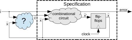
Figure 2: Circuit representation of a safety specification.

A safety specification expresses that certain “bad things” never happen in a system. We follow the framework of the SyntComp [21] synthesis competition, which defines safety specification benchmarks as hardware circuits in AIGER format, as illustrated in Figure 2. The circuits have uncontrollable inputs $\overline{i}$, controllable inputs $\overline{c}$, flip-flops to store a number of state bits $\overline{x}$, and one output “error” signaling specification violations. The corresponding synthesis problem is to construct a circuit that defines the controllable inputs $\overline{c}$ based on the uncontrollable inputs $\overline{i}$ and the state $\overline{x}$ in such a way that the error output can never become $\mathsf{true}$. This unknown circuit to be constructed is denoted with a question mark in Figure 2. We will also refer to the controllable inputs as control signals to emphasize that these signals are not intended to be inputs of the final system.

The specification illustrated in Figure 2 can be seen as a runtime monitor, declaratively encoding the design intent for the system to be synthesized. Another view is that the specification is a plant which needs to be controlled, or a sketch of a hardware circuit where the implementation for certain signals is still missing. Hence, this format flexibly fits various applications of synthesis. Formally, we define a safety specification as follows.

Definition 4 (Safety Specification)

A safety specification is a tuple $\mathcal{S}=(\overline{x},\overline{i},\overline{c},I,T,P)$, where

• $\overline{x}$ is a vector of Boolean state variables,

• $\overline{i}$ is a vector of uncontrollable, Boolean input variables,

• $\overline{c}$ is a vector of controllable, Boolean input variables,

• $I(\overline{x})$ is an initial condition, expressed as a propositional formula over the state variables,

• $T(\overline{x},\overline{i},\overline{c},\overline{x}^{\prime})$ is a transition relation, expressed as a propositional formula over the variables $\overline{x}$, $\overline{i}$, $\overline{c}$, and $\overline{x}^{\prime}$, where $\overline{x}^{\prime}$ denotes the next-state copy of $\overline{x}$,

• the transition relation $T(\overline{x},\overline{i},\overline{c},\overline{x}^{\prime})$ is complete in the sense that $\forall\overline{x},\overline{i},\overline{c}\operatorname{\mathbin{:}}\exists\overline{x}^{\prime}\operatorname{\mathbin{:}}T(\overline{x},\overline{i},\overline{c},\overline{x}^{\prime})$,

• $T$ is deterministic, meaning that $\forall\overline{x},\overline{i},\overline{c},\overline{x}_{1}^{\prime},\overline{x}_{2}^{\prime}\operatorname{\mathbin{:}}\bigl{(}T(\overline{x},\overline{i},\overline{c},\overline{x}_{1}^{\prime})\wedge T(\overline{x},\overline{i},\overline{c},\overline{x}_{2}^{\prime})\bigr{)}\rightarrow(\overline{x}_{1}^{\prime}=\overline{x}_{2}^{\prime})$, and

• $P(\overline{x})$ is a propositional formula representing the set of safe states in $\mathcal{S}$.

A state of $\mathcal{S}$ is an assignment to all state variables $\overline{x}$. We represent such assignments (and thus states ) as $\overline{x}$-minterms $\mathbf{x}$. In the spirit of symbolic encoding as introduced Section 2.3, a formula $F(\overline{x})$ over the state variables $\overline{x}$ represents the set of all states $\mathbf{x}$ for which $\mathbf{x}\models F(\overline{x})$ holds. In this way, the formula $I(\overline{x})$ defines a set of initial states, and $P(\overline{x})$ defines the safe states. Similarly, the formula $T$ defines allowed state transitions: a transition from the current state $\mathbf{x}$ to the next state $\mathbf{x}^{\prime}$ is allowed with input $\mathbf{i}$ and $\mathbf{c}$ iff $\mathbf{x}\wedge\mathbf{i}\wedge\mathbf{c}\wedge\mathbf{x}^{\prime}\models T(\overline{x},\overline{i},\overline{c},\overline{x}^{\prime})$. Definition 4 requires that the transition relation $T$ is both deterministic and complete. That is, for any state $\mathbf{x}$ and input $\mathbf{i},\mathbf{c}$, the next state $\mathbf{x}^{\prime}$ is uniquely defined.

2.4.2 Safety Games

A specification $\mathcal{S}=(\overline{x},\overline{i},\overline{c},I,T,P)$ can be seen as a game between two players: the environment and the system we wish to synthesize. Depending on the context, we will thus refer to $\mathcal{S}$ either as a specification or as a game.

Plays. The game starts in one of the initial states (chosen by the environment), and is played in rounds. In every round $j$, the environment first chooses an assignment $\mathbf{i}_{j}$ to the uncontrollable inputs $\overline{i}$. Next, the system picks an assignment $\mathbf{c}_{j}$ to the controllable inputs $\overline{c}$. The transition relation $T$ then computes the next state $\mathbf{x}_{j+1}$. This is repeated indefinitely. The resulting sequence $\mathbf{x}_{0},\mathbf{x}_{1}\ldots$ of states is called a play. Formally, we have that $\mathbf{x}_{0}\models I(\overline{x})$ and $\mathbf{x}_{j}\wedge\mathbf{x}_{j+1}^{\prime}\wedge T(\overline{x},\overline{i},\overline{c},\overline{x}^{\prime})$ is satisfiable (with some $\mathbf{i}_{j}$ and $\mathbf{c}_{j}$ chosen by the players) for all $j\geq 0$. A play $\mathbf{x}_{0},\mathbf{x}_{1}\ldots$ is won by the system and lost by the environment if $\forall j\operatorname{\mathbin{:}}\mathbf{x}_{j}\models P(\overline{x})$, i.e., if only safe states are visited. Otherwise, the play is lost by the system and won by the environment.

Preimages. Let $F(\overline{x})$ be a formula representing a certain set of states. The mixed preimage $\mathsf{Force}^{s}_{1}\bigl{(}F(\overline{x})\bigr{)}=\forall\overline{i}\operatorname{\mathbin{:}}\exists\overline{c},\overline{x}^{\prime}\operatorname{\mathbin{:}}T(\overline{x},\overline{i},\overline{c},\overline{x}^{\prime})\wedge F(\overline{x}^{\prime})$ represents all states from which the system can enforce that some state of $F$ is reached in exactly one step. Analogously, $\mathsf{Force}^{e}_{1}\bigl{(}F(\overline{x})\bigr{)}=\exists\overline{i}\operatorname{\mathbin{:}}\forall\overline{c}\operatorname{\mathbin{:}}\exists\overline{x}^{\prime}\operatorname{\mathbin{:}}T(\overline{x},\overline{i},\overline{c},\overline{x}^{\prime})\wedge F(\overline{x}^{\prime})$ gives all states from which the environment can enforce that $F$ is visited in one step. We also define the cooperative preimage $\mathsf{Reach}_{1}\bigl{(}F(\overline{x})\bigr{)}=\exists\overline{i},\overline{c},\overline{x}^{\prime}\operatorname{\mathbin{:}}T(\overline{x},\overline{i},\overline{c},\overline{x}^{\prime})\wedge F(\overline{x}^{\prime})$ denoting the set of all states from which $F$ can be reached cooperatively by the two players. The following dualities can easily be shown:

• $\neg\mathsf{Force}^{s}_{1}(F)=\mathsf{Force}^{e}_{1}(\neg F)$ holds because, intuitively, the states from which the system cannot enforce that $F$ is reached must be the states from which the environment can enforce that $\neg F$ is reached.

• $\neg\mathsf{Force}^{e}_{1}(F)=\mathsf{Force}^{s}_{1}(\neg F)$ holds because, dually, the states from which the environment cannot enforce that $F$ is reached must be the states from which the system can enforce that $\neg F$ is reached.

Furthermore, we have that $\mathsf{Reach}_{1}(F_{1})\vee\mathsf{Reach}_{1}(F_{2})=\mathsf{Reach}_{1}(F_{1}\vee F_{2})$. Yet, the following equivalence does not hold in general: $\mathsf{Force}^{s}_{1}(F_{1})\vee\mathsf{Force}^{s}_{1}(F_{2})=\!\!\!\!\!\!{\color[rgb]{1,0,0}\lightning}\;\mathsf{Force}^{s}_{1}(F_{1}\vee F_{2})$. The reason is that there may be states from which the environment controls whether $F_{1}$ or $F_{2}$ is visited next, and the system can only ensure that one of the two regions is reached. Such states falsify $\mathsf{Force}^{s}_{1}(F_{1}\vee F_{2})\rightarrow\mathsf{Force}^{s}_{1}(F_{1})\vee\mathsf{Force}^{s}_{1}(F_{2})$. This difference in compositionality between $\mathsf{Reach}_{1}$ and $\mathsf{Force}^{s}_{1}$ explains why some ideas from verification cannot be ported to synthesis straightforwardly.

Strategies. We focus on memoryless strategies because these strategies are sufficient for safety games [60]. A (memoryless) strategy for the system player in the game $\mathcal{S}$ is a formula $S(\overline{x},\overline{i},\overline{c},\overline{x}^{\prime})$ that specializes $T$ in the sense that

• $S(\overline{x},\overline{i},\overline{c},\overline{x}^{\prime})\rightarrow T(\overline{x},\overline{i},\overline{c},\overline{x}^{\prime})$ and

• $\forall\overline{x},\overline{i}\operatorname{\mathbin{:}}\exists\overline{c},\overline{x}^{\prime}\operatorname{\mathbin{:}}S(\overline{x},\overline{i},\overline{c},\overline{x}^{\prime}).$

The first bullet requires that the strategy may only allow state transitions that are also allowed by the transition relation. The second bullet requires the strategy to be complete with respect to the current state and uncontrollable input: for every state $\mathbf{x}$ and input $\mathbf{i}$, the strategy must contain some way to choose $\mathbf{c}$ (and some next state, but the next state is uniquely defined by $T$ already). For a particular situation, the strategy can allow many possibilities to choose $\mathbf{c}$, though. A strategy for the system is winning if all plays that can be constructed by following $S$ instead of $T$ are won by the system. The winning region $W(\overline{x})$ is the set of all states from which a winning strategy exists. That is, if the play would start in some arbitrary state of the winning region, the system player would have a strategy to win the game.

System implementations. A system implementation is a function $f:2^{\overline{x}}\times 2^{\overline{i}}\rightarrow 2^{\overline{c}}$ to uniquely define the control signals $\overline{c}$ based on the current state and the uncontrollable inputs $\overline{i}$. A system implementation $f$ implements a strategy $S$ if $\forall\overline{x},\overline{i}\operatorname{\mathbin{:}}\exists\overline{x}^{\prime}\operatorname{\mathbin{:}}S\bigl{(}\overline{x},\overline{i},f(\overline{x},\overline{i}),\overline{x}^{\prime}\bigr{)}$, that is, if for every state $\mathbf{x}$ and input $\mathbf{i}$, the control value $\mathbf{c}=f(\mathbf{x},\mathbf{i})$ computed by $f$ is allowed by the strategy $S$. A system implementation $f$ realizes a safety specification $\mathcal{S}=\bigl{(}\overline{x},\overline{i},\overline{c},I(\overline{x}),T(\overline{x},\overline{i},\overline{c},\overline{x}^{\prime}),P(\overline{x})\bigr{)}$ if all plays of $\mathcal{S}^{\prime}=\bigl{(}\overline{x},\overline{i},\emptyset,I(\overline{x}),T(\overline{x},\overline{i},f(\overline{x},\overline{i}),\overline{x}^{\prime}),P(\overline{x})\bigr{)}$ are won by the system player, i.e., visit only safe states. Here, $\mathcal{S}^{\prime}$ is a simplified version of the game $\mathcal{S}$ where the moves of the system player are defined by $f$, i.e., the system has no choices left. A safety specification is realizable if a system implementation that realizes it exists. Given a winning strategy $S$ for a safety specification $\mathcal{S}$, every implementation $f$ of the winning strategy $S$ realizes the specification $\mathcal{S}$. This follows from the definition of the winning strategy. Hence, a system implementation for a safety specification $\mathcal{S}$ can be constructed by computing a winning strategy $S$ for $\mathcal{S}$ and then computing an implementation $f$ of $S$.

2.4.3 Synthesis Algorithms for Safety Specifications

Given an explicit representation of the safety specification $\mathcal{S}$ as a game graph (with vertices representing states and edges representing state transition) the problem of deciding the realizability of a safety specification is solvable in linear time [60]. When starting from our symbolic representation $\mathcal{S}$, the problem is EXP-time complete [14].

A synthesis algorithm for safety specifications takes as input a safety specification $\mathcal{S}$ and computes a system implementation realizing this specification if such an implementation exists. If no such implementation exists, the algorithm reports unrealizability. Wolfgang Thomas [60] sketches the standard textbook algorithm for solving this problem. It proceeds in two steps. First, a winning strategy is computed. Second, the winning strategy is implemented in a circuit. This process is elaborated in the following two subsections.

2.4.4 Computing a Winning Strategy

The computation of a winning strategy $S(\overline{x},\overline{i},\overline{c},\overline{x}^{\prime})$ for the game $\mathcal{S}\!=\!\bigl{(}\overline{x},\overline{i},\overline{c},I(\overline{x}),T(\overline{x},\overline{i},\overline{c},\overline{x}^{\prime}),P(\overline{x})\bigr{)}$ is achieved by computing the winning region $W(\overline{x})$ of the game $\mathcal{S}$ using the procedure SafeWin, shown in Algorithm 1. The winning region $W$ is built up in the variable $F$. Initially, $F$ represents the set of all safe states $P$. Line 4 retains only those states of $F$ from which the system player can enforce that the play stays in a state of $F$ also in the next step. This operation is repeated as long as the state set $F$ changes. If the set of initial states $I$ is not contained in $F$ any more, the procedure aborts, returning $\mathsf{false}$ to signal unrealizability of the specification. Otherwise, the final version of $F$ is returned as the winning region. All operations that are performed in this algorithm can easily be realized using BDDs.

Algorithm 1 SafeWin: Computes a winning region in a safety game.

1:procedure SafeWin$\left((\overline{x},\overline{i},\overline{c},I,T,P)\right)$,     returns: The winning region or $\mathsf{false}$

2:   $F:=P$

3:   while $F$ changes do

4:      $F:=F\wedge\mathsf{Force}^{s}_{1}(F)$

5:      if $I\not\rightarrow F$ then

6:         return $\mathsf{false}$          

7:   return $F$

Algorithm 2 CofSynt: A cofactor-based algorithm for computing an implementation of a strategy.

1:procedure CofSynt$\left(S(\overline{x},\overline{i},\overline{c},\overline{x}^{\prime})\right)$, returns: $f_{1},\ldots,f_{n}:2^{\overline{x}}\times 2^{\overline{i}}\rightarrow\mathbb{B}$

2:   for $c_{j}\in\overline{c}$ do

3:      $C_{1}(\overline{x},\overline{i}):=\exists\overline{x}^{\prime},\overline{c}\operatorname{\mathbin{:}}S\bigl{(}\overline{x},\overline{i},(c_{0},\ldots,c_{j-1},\mathsf{true},c_{j+1},\ldots,c_{n}),\overline{x}^{\prime}\bigr{)}$

4:      $C_{0}(\overline{x},\overline{i}):=\exists\overline{x}^{\prime},\overline{c}\operatorname{\mathbin{:}}S\bigl{(}\overline{x},\overline{i},(c_{0},\ldots,c_{j-1},\mathsf{false},c_{j+1},\ldots,c_{n}),\overline{x}^{\prime}\bigr{)}$

5:      $C(\overline{x},\overline{i}):=\neg C_{1}(\overline{x},\overline{i})\vee\neg C_{0}(\overline{x},\overline{i})$

6:      $F_{j}(\overline{x},\overline{i}):=\textsf{simplify}(C_{1},C)$

7:      $S(\overline{x},\overline{i},\overline{c},\overline{x}^{\prime}):=S(\overline{x},\overline{i},\overline{c},\overline{x}^{\prime})\wedge\bigl{(}c_{j}\leftrightarrow F_{j}(\overline{x},\overline{i})\bigr{)}$    

8:   return $F_{1},\ldots,F_{n}$

If the specification is realizable, i.e., SafeWin did not return $\mathsf{false}$, a winning strategy $S$ is computed from the winning region $W$. For safety specifications, $S$ can be defined as $S(\overline{x},\overline{i},\overline{c},\overline{x}^{\prime})=T(\overline{x},\overline{i},\overline{c},\overline{x}^{\prime})\wedge\bigl{(}W(\overline{x})\rightarrow W(\overline{x}^{\prime})\bigr{)}.$ That is, the transition relation must always be respected. Furthermore, if the current state is in the winning region, then the next state must be contained in the winning region as well. This strategy will enforce the specification because $I\rightarrow W$, i.e., all initial states are contained in the winning region (otherwise SafeWin would have signaled unrealizability). When starting from a state of the winning region, the strategy ensures that the next state will be in the winning region again. Finally, the winning region $W$ can only contain safe states, i.e., $W\rightarrow P$. Hence, only safe states can be visited when following the strategy.

2.4.5 Computing a System Implementation from a Winning Strategy

The second step is to compute a system implementation that implements the strategy, and to realize this implementation in form of a circuit. This can be done by computing a Skolem function for the variables $\overline{c}$ in the formula $\forall\overline{x},\overline{i}\operatorname{\mathbin{:}}\exists\overline{c},\overline{x}^{\prime}\operatorname{\mathbin{:}}S(\overline{x},\overline{i},\overline{c},\overline{x}^{\prime}),$ i.e., a function $f:2^{\overline{x}}\times 2^{\overline{i}}\rightarrow 2^{\overline{c}}$ such that $\forall\overline{x},\overline{i}\operatorname{\mathbin{:}}\exists\overline{x}^{\prime}\operatorname{\mathbin{:}}S\bigl{(}\overline{x},\overline{i},f(\overline{x},\overline{i}),\overline{x}^{\prime}\bigr{)}$ holds. Usually, we prefer simple functions that can be implemented in small circuits. A survey of existing methods to solve this problem can be found in the work by Ehlers et al. [61]. One widely used method is presented in the following.

The cofactor-based method. The cofactor-based method presented by Bloem et al. [16] can be considered as the “standard method” for computing an implementation from a strategy. It is outlined in Algorithm 2. The input is a strategy $S$, the output is a set of functions $f_{1},\ldots,f_{n}:2^{\overline{x}}\times 2^{\overline{i}}\rightarrow\mathbb{B}$, each one defining one control signal of $\overline{c}=(c_{1},\ldots,c_{n})$. Together, these functions define $f:2^{\overline{x}}\times 2^{\overline{i}}\rightarrow 2^{\overline{c}}$. CofSynt computes one $f_{j}$ after the other. In Line 3, a formula $C_{1}(\overline{x},\overline{i})$ is constructed. It represents the set of all valuations of $\overline{x}$ and $\overline{i}$ in which $c_{j}=\mathsf{true}$ is allowed by the strategy. It is computed as the positive cofactor of $S$ with respect to $c_{j}$, while all signals that are currently not relevant are quantified existentially. Similarly, Line 4 computes all situations where $c_{j}=\mathsf{false}$ is allowed by the strategy. Our definition of a strategy implies that $C_{1}(\overline{x},\overline{i})\vee C_{0}(\overline{x},\overline{i})=\mathsf{true}$, i.e., one of the two values is always allowed (but sometimes both are allowed). Next, Line 5 computes the care set $C$, i.e., the set of all situations in which the output matters. Outside of this care set, the value of $c_{j}$ can be set arbitrarily. Line 6 uses this information to simplify $C_{1}$: The procedure simplify returns some $F_{j}$ which is equal to $C_{1}$ wherever $C$ is $\mathsf{true}$, and arbitrary where $C$ is $\mathsf{false}$. When using BDDs as reasoning engine, this simplification can be implemented with the operation Restrict [62]. However, this is an optional optimization to obtain smaller circuits. Setting $F_{j}=C_{1}$ would work as well. Finally, Line 7 refines the strategy $S$ with the computed implementation for the control signal $c_{j}$. This step is necessary because some control signals may depend on others, so fixing the implementation of one control signal may restrict other control signals.

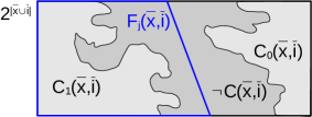
Figure 3: Working principle of CofSynt.

Illustration. Figure 3 illustrates one iteration of the CofSynt procedure graphically. The box represents the set of all possible assignments to the variables $\overline{x}$ and $\overline{i}$. The region $C_{1}$ contains all situations where $c_{j}=\mathsf{true}$ is allowed. Similarly, $C_{0}$ contains all situations where $c_{j}=\mathsf{false}$ is allowed. The overlap of the two regions is colored in dark gray. Hence, the dark gray region is the set of situations where both $c_{j}=\mathsf{true}$ and $c_{j}=\mathsf{false}$ is allowed. It corresponds to the negation $\neg C$ of the care set $C$. Note that each point in the box is either contained in $C_{1}$ or in $C_{0}$ (or in both). The function $F_{j}$ defining $c_{j}$ is shown in blue. Outside of the dark gray don’t-care area $\neg C$ it matches $C_{1}$ precisely. In the don’t-care area it can be different, though. These properties are enforced by the procedure simplify, called in Line 6 of CofSynt. Exploiting the freedom in the don’t-care region can result in simpler formulas and thus in smaller circuits. In Figure 3, this is indicated by $F_{j}$ being much more regular than $C_{1}$.

Computing circuits. In order to obtain an implementation $f$ in form of a hardware circuit, the individual functions $f_{j}$, defined as formulas $F_{j}$, need to be transformed into a network of gates. In principle, this is not difficult: each $F_{j}$ is a propositional formula (if quantifiers are left, they can be expanded) and the structure of the formula can directly be translated into gates. If BDDs are used, each BDD node can be translated into a multiplexer.

2.5 Learning by Queries

In this section, we discuss concepts for learning propositional formulas based on queries, as introduced by Angluin [23]. We refer to Crama and Hammer [63, Chapter 7] for a more elaborate discussion.

2.5.1 Basic Concept

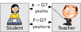
Figure 4: Student and teacher in query learning.

The goal of query learning is to compute a small representation $F$ of a propositional formula $G(\overline{x})$ over a given set $\overline{x}$ of Boolean variables. As illustrated in Figure 4, this is achieved by two parties in interaction: the student (or learner) and the teacher (or oracle). The student can ask two kinds of questions:

• A subset query asks if a given (potentially incomplete) cube $\mathbf{x}$ is fully contained in $G(\overline{x})$, i.e., if the implication $\mathbf{x}\rightarrow G$ holds. The answer to this question is either yes or no. In algorithms, we will denote such queries by $\mathsf{SUB}(\mathbf{x},G)$.

• An equivalence query asks if a given candidate formula $F(\overline{x})$ is equivalent to $G(\overline{x})$. The answer is again either yes or no. However, in the no-case, the teacher also returns a counterexample $\mathbf{x}$ in form of an $\overline{x}$-minterm witnessing the difference. A counterexample is either a false-positive with $\mathbf{x}\models F$ and $\mathbf{x}\not\models G$ or a false-negative with $\mathbf{x}\not\models F$ and $\mathbf{x}\models G$. In algorithms, we will denote equivalence queries by $\mathsf{EQ}(F,G)$.

A membership query is a special form of a subset query where $\mathbf{x}$ is an $\overline{x}$-minterm, i.e., a complete cube.

2.5.2 Learning Algorithms

The general pattern for query learning algorithms is that they start with some initial “guess” of the target function. In a loop, they then perform equivalence queries. If counterexamples are returned, the guess of the target function is refined to eliminate the counterexample. The refinement may involve membership- and subset queries, and distinguishes the algorithms. Concrete algorithms are presented in the following.

Algorithm 3 DnfLearn: A DNF learning algorithm.

1:procedure DnfLearn$\left(G(\overline{x})\right)$,                              returns: A DNF representation $F(\overline{x})$ of $G(\overline{x})$

2:   $F:=\mathsf{false}$

3:   while $\mathsf{EQ}(F,G)$ returns a counterexample $\mathbf{x}$ do

4:      $\mathbf{x}_{g}:=\mathbf{x}$

5:      for each literal $l$ in $\mathbf{x}$ do

6:         if $\mathsf{SUB}(\mathbf{x}_{g}\setminus\{l\},G)$ then

7:            $\mathbf{x}_{g}:=\mathbf{x}_{g}\setminus\{l\}$                

8:      $F:=F\vee\mathbf{x}_{g}$    

9:   return $F$

Algorithm 4 CnfLearn: A CNF learning algorithm.

1:procedure CnfLearn$\left(G(\overline{x})\right)$,                              returns: A CNF representation $F(\overline{x})$ of $G(\overline{x})$

2:   $F:=\mathsf{true}$

3:   while $\mathsf{EQ}(F,G)$ returns a counterexample $\mathbf{x}$ do

4:      $\mathbf{x}_{g}:=\mathbf{x}$

5:      for each literal $l$ in $\mathbf{x}$ do

6:         if $\mathsf{SUB}(\mathbf{x}_{g}\setminus\{l\},\neg G)$ then

7:            $\mathbf{x}_{g}:=\mathbf{x}_{g}\setminus\{l\}$                

8:      $F:=F\wedge\neg\mathbf{x}_{g}$    

9:   return $F$

Learning a DNF. DnfLearn [63, Chapter 7] in Algorithm 3 computes a DNF representation of a given formula $G(\overline{x})$ using equivalence- and subset queries. It starts with the initial guess $F=\mathsf{false}$. This guess is then refined based on the counterexamples returned by the equivalence queries in Line 3. The algorithm maintains the invariant $F\rightarrow G$. Hence, a counterexample $\mathbf{x}$ can only be a false-negative, i.e., $\mathbf{x}\not\models F$ but $\mathbf{x}\models G$. In principle, the counterexample $\mathbf{x}$ can be eliminated by updating $F$ to $F\vee\mathbf{x}$ without executing the inner for-loop. However, in order to (potentially) reduce the number of iterations and also the size of $F$, the counterexamples are generalized: The inner loop drops literals from the cube $\mathbf{x}$ as long as the reduced cube $\mathbf{x}_{g}$ still implies $G$, i.e., represents only variable assignments that must be mapped to $\mathsf{true}$ in the end. Thus, the subsequent update $F:=F\vee\mathbf{x}_{g}$ does not only eliminate the original counterexample $\mathbf{x}$, but may also eliminate many other counterexamples that have not been encountered yet. Note that this inner loop actually computes an unsatisfiable core $\mathbf{x}_{g}:=\textsc{PropMinUnsatCore}(\mathbf{x},\neg G)$. If no more counterexamples are left, the algorithm terminates and returns $F$, which is a disjunction of cubes, i.e., a DNF that is equivalent to $G$.

Learning a CNF. A CNF representation of a given formula $G(\overline{x})$ can be computed with $F=\neg\textsc{DnfLearn}(\neg G)$, i.e., by computing a DNF for $\neg G$ and negating the result. Alternatively, the procedure DnfLearn can easily be rewritten to compute CNFs directly. This is shown in Algorithm 4. The working principle remains the same, but $F$ is initialized to $\mathsf{true}$ and refined with clauses that are computed from the false-positives returned by the equivalence queries.

More query learning algorithms can be found in the literature. For instance, an algorithm to learn formulas in form of a conjunction of DNFs can be defined using Bshouty’s monotone theory [64]. Ehlers et al. [61] show how various learning algorithms can be used effectively in circuit synthesis using BDDs. In this article we focus on satisfiability-based synthesis methods. SAT- and QBF solvers operate on CNF representations of a formula. Hence, our algorithms will mostly rely on the CNF learning approach. We therefore refrain from introducing more complicated learning methods here in detail, and refer the interested reader to the book by Crama and Hammer [63, Chapter 7].

2.6 Counterexample-Guided Inductive Synthesis (CEGIS)

The basic principle of query learning, namely refining an initial “guess” of the solution iteratively based on counterexamples, has also been applied to other synthesis-related problems. One example is Counterexample-Guided Inductive Synthesis (CEGIS) [4, 5], which was introduced in the context of program sketching as a method to compute satisfying assignments for quantified formulas of the form $\exists\overline{e}\operatorname{\mathbin{:}}\forall\overline{u}\operatorname{\mathbin{:}}F(\overline{e},\overline{u}).$ The goal is to compute concrete values $\mathbf{e}$ for the variables $\overline{e}$ such that $\forall\overline{u}\operatorname{\mathbin{:}}F(\mathbf{e},\overline{u})$ holds. While the general principle is independent of the logic, we will assume that $F$ is a propositional formula. Hence, $\overline{e}$ and $\overline{u}$ are vectors of Boolean variables, and we can use a SAT solver to reason about $F$ (without the quantifiers).

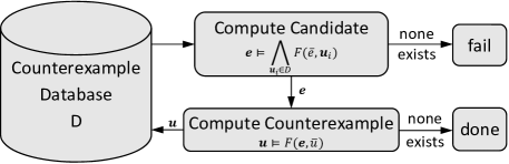
Figure 5: Working principle of CEGIS.

Working principle. Similar to query learning, a candidate $\mathbf{e}$ for a solution is iteratively refined based on counterexamples, which are concrete assignments to the variables $\overline{u}$ witnessing that $\forall\overline{u}\operatorname{\mathbin{:}}F(\mathbf{e},\overline{u})$ does not yet hold. This refinement loop is illustrated in Figure 5. There is a database $D$ of counterexamples $\mathbf{u}_{i}$, which is initially empty. The first step of the loop is to compute a candidate assignment $\mathbf{e}\models\bigwedge_{\mathbf{u}_{i}\in D}F(\overline{e},\mathbf{u}_{i})$ that satisfies $F$ for all counterexamples that have been encountered previously. This is a necessary but not a sufficient condition for $\forall\overline{u}\operatorname{\mathbin{:}}F(\mathbf{e},\overline{u})$. Hence, if no such candidate $\mathbf{e}$ exists, this means that $\exists\overline{e}\operatorname{\mathbin{:}}\forall\overline{u}\operatorname{\mathbin{:}}F(\overline{e},\overline{u})$ is unsatisfiable, so the algorithm aborts. If a candidate $\mathbf{e}$ was found, the next step is to check if $F(\mathbf{e},\overline{u})$ holds for all $\overline{u}$ and not just for the concrete $\overline{u}$-values stored in $D$. This check is performed by searching for a counterexample $\mathbf{u}\models\neg F(\mathbf{e},\overline{u})$ for which $F$ does not (yet) hold with the given $\mathbf{e}$. If no such counterexample exists, then $\mathbf{e}$ must be a solution, and the algorithm terminates. Otherwise, the counterexample $\mathbf{u}$ is added to $D$ and another iteration is performed. The candidate that is computed in the next iteration is already “better” in the sense that it satisfies $F$ also for the counterexample from the previous iteration (and all iterations before). For a propositional formula $F$ over finite vectors $\overline{e}$ and $\overline{u}$ of Boolean variables, the CEGIS algorithm must terminate eventually. The reason is that every iteration excludes (at least) one candidate. Moreover, there is only a finite set of counterexamples to encounter.

Algorithm 5 CegisSat: CEGIS implemented using a SAT solver.

1:procedure CegisSat$\left(F(\overline{e},\overline{u})\right)$,                                           returns: An assignment $\mathbf{e}$ for $\overline{e}$ such that $\forall\overline{u}\operatorname{\mathbin{:}}F(\mathbf{e},\overline{u})$ or “fail”

2:   $G(\overline{e}):=\mathsf{true}$

3:   while $\mathsf{true}$ do

4:      if $\textsf{sat}=\mathsf{false}$ in $(\textsf{sat},\mathbf{e}):=\textsc{PropSatModel}\bigl{(}G(\overline{e})\bigr{)}$  then

5:         return “fail”       

6:      if $\textsf{sat}=\mathsf{false}$ in $(\textsf{sat},\mathbf{u}):=\textsc{PropSatModel}\bigl{(}\neg F(\mathbf{e},\overline{u})\bigr{)}$  then

7:         return $\mathbf{e}$       

8:      $G(\overline{e}):=G(\overline{e})\wedge F(\overline{e},\mathbf{u})$    

Algorithm. Algorithm 5 implements CEGIS using a SAT solver. Line 4 computes candidates and Line 6 performs the candidate check as well as the counterexample computation in the straightforward way. Instead of storing a database of counterexamples, the algorithm directly refines the constraints for a candidate in Line 8. Note that constraints are only added to $G$, so the algorithm is well suited for incremental solving.

3 From Safety Specifications to Strategies

As discussed in Section 2.4.3, a strategy $S$ for realizing a safety specification $\mathcal{S}=\bigl{(}\overline{x},\overline{i},\overline{c},I(\overline{x}),$ $T(\overline{x},\overline{i},\overline{c},\overline{x}^{\prime}),P(\overline{x})\bigr{)}$ can be constructed by computing the winning region $W(\overline{x})$ in the game defined by $\mathcal{S}$. Recall that the winning region is the set of all states from which the system player can enforce that only safe states are visited. Once the winning region is available, the corresponding strategy can be defined as $S(\overline{x},\overline{i},\overline{c},\overline{x}^{\prime})=T(\overline{x},\overline{i},\overline{c},\overline{x}^{\prime})\wedge\bigl{(}W(\overline{x})\rightarrow W(\overline{x}^{\prime})\bigr{)}.$ However, a winning strategy can also be computed by different means. One option is to use a winning area, defined as follows.

Definition 5 (Winning Area)

A winning area for a safety specification $\mathcal{S}=\bigl{(}\overline{x},\overline{i},\overline{c},I(\overline{x}),T(\overline{x},\overline{i},\overline{c},\overline{x}^{\prime}),$ $P(\overline{x})\bigr{)}$ is a state set $F$, represented symbolically as a formula $F(\overline{x})$, with the following three properties:

• Every initial state is contained in $F$, i.e., $I(\overline{x})\rightarrow F(\overline{x})$.

• $F$ contains only safe states, i.e., $F(\overline{x})\rightarrow P(\overline{x})$.

• The system player can enforce that the play stays in $F$, i.e., $F(\overline{x})\rightarrow\mathsf{Force}^{s}_{1}\bigl{(}F(\overline{x})\bigr{)}$.

These properties are sufficient to ensure that $T(\overline{x},\overline{i},\overline{c},\overline{x}^{\prime})\wedge\bigl{(}F(\overline{x})\rightarrow F(\overline{x}^{\prime})\bigr{)}$ is a winning strategy. The reason is the same as for the winning region (Section 2.4.4): the control signals can always be set such that the next state is in $F$ again, and $F$ contains only safe states. In fact, the winning region is just a special winning area, namely the largest one.

The following sections will present different methods for computing the winning region or a winning area using decision procedures for the satisfiability of formulas. We will use the terms “satisfiability-based” or “SAT-based” to indicate the use of any such decision procedures, including SAT-, QBF- and EPR solvers. We will write “SAT solver based” to specifically indicate the use of propositional SAT solvers.

3.1 QBF-Based Learning

The SafeWin procedure presented in Algorithm 1 can be implemented with BDDs using their capability of quantifier elimination in a rather straightforward manner. However, a realization with plain SAT solvers is not easily possible because the preimage operation $\mathsf{Force}^{s}_{1}$ in Line 4 contains a universal quantification. Therefore, a natural option is to use a QBF solver, which can handle universal quantifications without expanding the formula.

3.1.1 A Straightforward QBF Realization of SafeWin

A direct realization of SafeWin with QBF solving was presented by Staber and Bloem [65]. We briefly review this existing method and its drawbacks before presenting our learning-based algorithms. For this discussion, we will refer to the different values of the variable $F$ in Algorithm 1 with indices. That is, $F_{0}=P$ denotes the initial value of $F$ and $F_{j}=F_{j-1}\wedge\mathsf{Force}^{s}_{1}(F_{j-1})$ is the value after the $j$^th iteration. The termination check in Line 3 is performed by checking two subsequent values $F_{j}$ and $F_{j-1}$ for equivalence. Since $F_{j}\rightarrow F_{j-1}$, i.e., the set $F$ of states can only get smaller from iteration to iteration, it is sufficient to check if $F_{j-1}\rightarrow F_{j}$. Thus, the first check of “F changes” can be realized with the QBF query $\neg\textsc{QbfSat}\bigl{(}\forall\overline{x},\overline{i}\operatorname{\mathbin{:}}\exists\overline{c},\overline{x}^{\prime}\operatorname{\mathbin{:}}P(\overline{x})\rightarrow\bigl{(}T(\overline{x},\overline{i},\overline{c},\overline{x}^{\prime})\wedge P(\overline{x}^{\prime})\bigr{)}\bigr{)}.$ The second check if $F$ changes translates to $\neg\textsc{QbfSat}\bigl{(}\forall\overline{x},\overline{i}\operatorname{\mathbin{:}}\exists\overline{c},\overline{x}^{\prime}\operatorname{\mathbin{:}}\forall\overline{i}^{\prime}\operatorname{\mathbin{:}}\exists\overline{c}^{\prime},\overline{x}^{\prime\prime}\operatorname{\mathbin{:}}\bigl{(}P(\overline{x})\wedge T(\overline{x},\overline{i},\overline{c},\overline{x}^{\prime})\wedge P(\overline{x}^{\prime})\bigr{)}\rightarrow\bigl{(}T(\overline{x}^{\prime},\overline{i}^{\prime},\overline{c}^{\prime},\overline{x}^{\prime\prime})\wedge P(\overline{x}^{\prime\prime})\bigr{)}\bigr{)},$ and so on. In general, the check if $F$ changed in iteration $j$ requires solving a QBF with $2\cdot j-1$ quantifier alternations and $j$ copies of the transition relation $T$. The checks if $I\rightarrow F_{j}$ in Line 5 of Algorithm 1 work in a similar way, also requiring $2\cdot j-1$ quantifier alternations and $j$ copies of the transition relation. We consider this steep increase in formula size and complexity as suboptimal. In the following, we will therefore present algorithms that require only one copy of the transition relation and a constant number of quantifier alternations in the queries to the QBF solver.

3.1.2 A QBF-Based CNF Learning Algorithm

Algorithm 6 QbfWin: Basic QBF-based CNF learning algorithm for the winning region.

1:procedure QbfWin$\left((\overline{x},\overline{i},\overline{c},I,T,P)\right)$, returns: The winning region $W(\overline{x})$ in CNF or $\mathsf{false}$

2:   if $\textsc{PropSat}\bigl{(}I(\overline{x})\wedge\neg P(\overline{x})\bigr{)}$ then return $\mathsf{false}$

3:   $F(\overline{x}):=P(\overline{x})$

4:   while $\mathsf{sat}=\mathsf{true}$ in $(\mathsf{sat},\mathbf{x}):=\textsc{QbfSatModel}\bigl{(}\exists\overline{x},\overline{i}\operatorname{\mathbin{:}}\forall\overline{c}\operatorname{\mathbin{:}}\exists\overline{x}^{\prime}\operatorname{\mathbin{:}}F(\overline{x})\wedge T(\overline{x},\overline{i},\overline{c},\overline{x}^{\prime})\wedge\neg F(\overline{x}^{\prime})\bigr{)}$ do

5:      $\mathbf{x}_{g}:=\mathbf{x}$

6:      for each literal $l$ in $\mathbf{x}$ do

7:         $\mathbf{x}_{t}:=\mathbf{x}_{g}\setminus\{l\}$

8:         if $\neg\textsc{QbfSat}\bigl{(}\exists\overline{x}\operatorname{\mathbin{:}}\forall\overline{i}\operatorname{\mathbin{:}}\exists\overline{c},\overline{x}^{\prime}\operatorname{\mathbin{:}}\mathbf{x}_{t}\wedge F(\overline{x})\wedge T(\overline{x},\overline{i},\overline{c},\overline{x}^{\prime})\wedge F(\overline{x}^{\prime})\bigr{)}$ then

9:            $\mathbf{x}_{g}:=\mathbf{x}_{t}$                

10:      if $\textsc{PropSat}\bigl{(}\mathbf{x}_{g}\wedge I(\overline{x})\bigr{)}$ then return $\mathsf{false}$

11:      $F(\overline{x}):=F(\overline{x})\wedge\neg\mathbf{x}_{g}$    

12:   return $F(\overline{x})$

Algorithm 6 shows the procedure QbfWin, which computes a CNF representation of the winning region $W(\overline{x})$ using CNF learning with a QBF solver. Since QbfWin will also be the basis for our algorithms that use plain SAT solving, we discuss it here in detail. Just like SafeWin in Algorithm 1, QbfWin takes a specification as input. It returns either the winning region $W(\overline{x})$ or $\mathsf{false}$ in case of unrealizability. The basic structure is that of the CNF learning procedure CnfLearn in Algorithm 4. However, in Line 3, $F$ is initialized to $P$ instead of $\mathsf{true}$ because the winning region can only be a subset of the safe states $P$. Differences in counterexample computation and generalization are discussed in the following.

Counterexample computation. The equivalence query in Line 3 of the original CNF learning procedure CnfLearn asks if the current approximation of the solution is correct. The corresponding line (Line 4) in QbfWin now checks if $F\rightarrow\mathsf{Force}^{s}_{1}(F)$ is valid, i.e., if another visit of $F$ can be enforced by the system from any state of $F$. The QBF query in Line 4 of QbfWin actually asks the opposite question, namely if there exists a state $\mathbf{x}$ in $F$ from which the environment can enforce leaving $F$, i.e., if $F\wedge\mathsf{Force}^{e}_{1}(\neg F)$ is satisfiable. This is the case if there exists some state $\mathbf{x}$ in $F$ and some input $\mathbf{i}$ such that for all control values $\mathbf{c}$ the next state will be in $\neg F$. If such a state $\mathbf{x}$ exists, QbfSatModel will return it as a counterexample witnessing that $F$ is not equal to the winning region $W$. More specifically, this state $\mathbf{x}$ cannot be part of $W$, and thus needs to be removed from $F$. This removal is performed in Line 11. However, in order to reduce the number of iterations, the counterexample is generalized beforehand. This is explained in the next paragraph. If, on the other hand, QbfSatModel sets sat to $\mathsf{false}$ in Line 4, then this means that the implication $F\rightarrow\mathsf{Force}^{s}_{1}(F)$ holds. In this case, QbfWin terminates, returning $F$ as the winning region.

Counterexample generalization. Just like in CnfLearn, counterexample generalization is done by eliminating literals of $\mathbf{x}$ in the inner loop of the algorithm. In CnfLearn (see Algorithm 4), the final cube $\mathbf{x}_{g}\subseteq\mathbf{x}$ must not intersect with $G$ in order not to shrink $F$ beyond $G$. Similarly, in QbfWin, $\mathbf{x}_{g}\wedge F$ must not intersect with $\mathsf{Force}^{s}_{1}(F)$ in order not to remove any states from the winning region where the system could enforce that the play stays in the winning region. The reason is that the subsequent update $F:=F\wedge\neg\mathbf{x}_{g}$ in Line 11 removes exactly the states $\mathbf{x}_{g}\wedge F$. The QBF query in Line 8 is satisfiable if $\mathbf{x}_{t}\wedge F$ contains any states of $\mathsf{Force}^{s}_{1}(F)$, and thus prevents unjust state removals. Also note that the inner loop essentially computes an unsatisfiable core of $\mathbf{x}$ with respect to $F\wedge\mathsf{Force}^{s}_{1}(F)$.

Detecting unrealizability. Detecting unrealizability is simple. The specification is unrealizable if and only if some initial state is outside of the winning region, i.e., if $I\not\rightarrow W$. The reason is that no system implementation can prevent the environment from visiting an unsafe state from an initial state that is not winning. QbfWin returns $\mathsf{false}$ as soon as $I\not\rightarrow F$. Since $F=W$ eventually, this ensures that $\mathsf{false}$ is returned if $I\not\rightarrow W$. Line 2 checks if $I\not\rightarrow F$ would hold initially. In every iteration, Line 10 then checks if the states $\mathbf{x}_{g}$ that are going to be removed from $F$ contain an initial state. This is potentially more efficient than than checking $I\not\rightarrow F$ again.

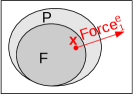
(a) Counterexample computation.

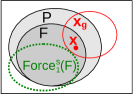
(b) Generalization.

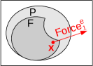
(c) Update of $F$.

Figure 6: Working principle of QbfWin.

Illustration. Figure 6 illustrates the working principle of QbfWin graphically. A box represents the set of all states. $F$ is always a subset of $P$. In Figure 6a, a counterexample $\mathbf{x}\models F\wedge\mathsf{Force}^{e}_{1}(\neg F)$ is computed. It represents a state from which the environment can enforce that $F$ is left. Next, the counterexample $\mathbf{x}$ is generalized into a larger region $\mathbf{x}_{g}$ by eliminating literals, as illustrated in Figure 6b. Every literal that can be eliminating from $\mathbf{x}$ doubles the size of the state region that is represented by $\mathbf{x}_{g}$. Literals are dropped as long as $\mathbf{x}_{g}\wedge F$ does not intersect with $\mathsf{Force}^{s}_{1}(F)$. Finally, as illustrated in Figure 6c, the generalized counterexample $\mathbf{x}_{g}$ is removed from $F$ and the next counterexample is computed. This is repeated until no more counterexamples exist, or one of the initial states is removed.

The following theorem summarizes these explanations into a formal correctness argument.

Theorem 6

The QbfWin procedure in Algorithm 6 returns the winning region $W(\overline{x})$ of a given safety specification $\mathcal{S}$, or $\mathsf{false}$ if the specification is unrealizable.

Proof 1

QbfWin enforces the invariants $F\rightarrow P$ (through Lines 3 and 11) and $I\rightarrow F$ (through Lines 2 and 10). The loop terminates normally if $F\rightarrow\mathsf{Force}^{s}_{1}(F)$. Hence, upon normal termination, $F$ is certainly a winning area according to Definition 5. $F$ is also the largest possible winning area, and thereby the winning region, because QbfWin also enforces the invariant $W\rightarrow F$. This invariant can be proven by induction: Initially $F=P$, so $W\rightarrow F$ holds because $W\rightarrow P$. Under the hypothesis that $W\rightarrow F$ holds before an update of $F$ in Line 11, it will also hold after the update because Line 11 only removes states $\mathbf{x}_{g}\wedge F$ for which $\mathbf{x}_{g}\wedge F\rightarrow\mathsf{Force}^{e}_{1}(\neg F)$ holds. Given that $W\rightarrow F$, we have that $\neg F\rightarrow\neg W$. This means that $\mathbf{x}_{g}\wedge F\rightarrow\mathsf{Force}^{e}_{1}(\neg W)$, so only states that cannot be part of $W$ are removed. QbfWin will always terminate because in every iteration, at least one state is removed from $F$, and when $F$ reaches $\mathsf{false}$ (or earlier) the loop necessarily terminates. What remains to be shown is that QbfWin aborts in Line 2 or 10 iff $\mathcal{S}$ is unrealizable, i.e., iff $I\not\rightarrow W$. (Direction $\Rightarrow$:) Since $W\rightarrow F$, and Line 2 or 10 abort iff ($F$ is about to be updated in such a way that) $I\not\rightarrow F$, it follows that QbfWin can only abort if $I\not\rightarrow W$. (Direction $\Leftarrow$:) Since $F=W$ eventually, Line 2 or 10 will definitely abort eventually if $I\not\rightarrow W$.

Discussion. In contrast to the approach from Section 3.1.1, all QBF queries in QbfWin contain only one copy of the transition relation and only two quantifier alternations. This potentially increases the scalability with respect to the size of the specifications. The disadvantage is that the number of calls to the QBF solver can be significantly higher.

3.1.3 Variants and Improvements

In this section, we now discuss a few variants and optimizations of QbfWin as presented in Algorithm 6.

Better generalization. At any point in the inner loop of QbfWin, $\mathbf{x}_{g}$ represents states that will definitely be removed from $F$. This information can be exploited already during the generalization loop by modifying the QBF query in Line 8 to $\neg\textsc{QbfSat}\bigl{(}\exists\overline{x}\operatorname{\mathbin{:}}\forall\overline{i}\operatorname{\mathbin{:}}\exists\overline{c},\overline{x}^{\prime}\operatorname{\mathbin{:}}\mathbf{x}_{t}\wedge F(\overline{x})\wedge\neg\mathbf{x}_{g}\wedge T(\overline{x},\overline{i},\overline{c},\overline{x}^{\prime})\wedge F(\overline{x}^{\prime})\wedge\neg\mathbf{x}_{g}^{\prime}\bigr{)}.$ This way, the generalization loop behaves as if $F$ would have been refined to $F(\overline{x})\wedge\neg\mathbf{x}_{g}$ already (with the current version of $\mathbf{x}_{g}$). The QBF query becomes stricter, which can have the effect that more literals can be eliminated. This can reduce the total number of counterexamples that have to be resolved. In the illustration of Figure 6b, this optimization shrinks $\mathsf{Force}^{s}_{1}(F)$ to $\mathsf{Force}^{s}_{1}(F\wedge\mathbf{x}_{g})$, which allows $\mathbf{x}_{g}$ to grow even larger. Since this optimization does not increase the number or complexity of the QBF queries, we always apply it.

Generalization until fixpoint. With the generalization optimization from the previous paragraph, the generalization check becomes non-monotonic in the sense that, even if a literal could not be eliminated initially, it may be eliminable after eliminating other literals. Hence, it can be beneficial to repeat the generalization loop until a fixpoint is reached. However, in our experiments, this did not result in noticeable performance improvements on the average over our benchmarks, so this is not done by default.

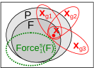
Figure 7: Computing all counterexample generalizations in QbfWin.

Computing all counterexample generalizations. In our experiments we observed that counterexample computation often takes much more time than counterexample generalization. Moreover, depending on the order in which the literals $l\in\mathbf{x}$ are processed in Line 6 of QbfWin, we can get different generalizations $\mathbf{x}_{g}$. Motivated by these observations, we propose a variant that computes all minimal generalizations for each counterexample. A naive solution would just run the generalization loop of Line 6 repeatedly using all $|\mathbf{x}|!$ different orders of the literals in $\mathbf{x}$. However, since many orderings can result in the same generalization $\mathbf{x}_{g}$, this is potentially inefficient. Instead, we thus apply an adaption of the hitting set tree algorithm presented by Reiter [66]. For the sake of readability, we refrain from presenting this algorithm in detail. The high-level intuition is visualized in Figure 7. All generalizations $\mathbf{x}_{g1}$, $\mathbf{x}_{g2}$ and $\mathbf{x}_{g3}$ will contain the original counterexample $\mathbf{x}$, and none of them may intersect with $\mathsf{Force}^{s}_{1}(F)$ inside of $F$. Although there may be a significant overlap between the generalizations, removing all of them prunes $F$ more than removing just one of them. In our experiments, we observed that the number of different counterexample generalizations is usually low. Not infrequently, there is only exactly one minimal generalization. Of course, computing all generalizations costs additional computation time. In our experiments, it gives a solid speedup for some benchmarks, but slows down the computation for others. Hence, we do not apply this optimization by default. Instead of computing all generalizations, one could also compute and apply at most $k$ different generalizations for some value of $k$. Another option is to compute all generalizations but refine $F$ only with the $k$ shortest ones. However, in preliminary experiments, these variants did not result in significant performance increases either.

3.1.4 Efficient Implementation

In this section, we give a few remarks on implementing QbfWin efficiently.

CNF encoding. The transition relation $T$, the characterization of the safe states $P$ and the formula for the initial states $I$ are transformed into CNF initially. Furthermore, a CNF representation of $\neg F$ needs to be computed in each iteration. All these transformations can be done using the method of Plaisted and Greenbaum [31]. This may introduce additional auxiliary variables, which are quantified existentially on the innermost level of the QBF queries. Once $T$, $P$, $I$ and $\neg F$ are available in CNF, the matrices of the QBF queries in Algorithm 6 can be constructed by building the union of the respective clause sets, because the individual formula parts are all connected by conjunctions.

CNF compression. After some iterations, the CNF formula $F$ in QbfWin can contain redundant clauses and literals. First, a clause discovered in some later iteration can be a proper subset of some earlier discovered clause. This can be checked syntactically at low costs. Thus, whenever a clauses is added to $F$, we always remove all of its supersets. Second, a set of clauses may together imply clauses that have been added earlier. The implied clauses can be eliminated without changing $F$ semantically. Third, it may be possible to drop literals from clauses of $F$ in an equivalence-preserving manner. The procedure CompressCnf in Algorithm 7 performs these simplifications and is explained in the next paragraph. We call this procedure to simplify $F$ after every modification of $F$, but with literal dropping disabled (we will later use CompressCnf with literal dropping enabled in other contexts). CompressCnf is very fast compared to the QBF solver calls in QbfWin. Furthermore, a smaller CNF representation of $F$ is particularly important for computing a compact representation of $\neg F$ using the method of Plaisted and Greenbaum [31]. Ultimately, the more compact CNF representations reduce the QBF solving time quite significantly.

Algorithm 7 CompressCnf: Removing redundant literals and clauses from a CNF.

1:procedure CompressCnf$\left(F(\overline{x})\right)$,                              returns: An equivalent but potentially smaller CNF $G(\overline{x})$

2:   if dropping literals enabled then

3:      $G:=\mathsf{true}$

4:      for each clause $c$ in $F$ do

5:         $G:=G\wedge\neg\textsc{PropMinUnsatCore}(\neg c,F)$       

6:      $F:=G$    

7:   $G:=\mathsf{true}$

8:   for each clause $c$ in $F$ with increasing size do

9:      if $\textsc{PropSat}(G\wedge\neg c)$ then

10:         $G:=G\wedge c$          

11:   return $G$

An algorithm for CNF compression. Algorithm 7 uses a SAT solver to remove redundant literals and clauses from a CNF formula $F(\overline{x})$. The first loop (if enabled) drops literals from each clause $c$ as long as the reduced clause $c_{2}\subseteq c$ is still implied by $F$. This ensures that the reduced formula $G$ is implied by $F$. Dropping literals can only make the formula stronger, i.e., $F$ is necessarily implied by $G$. Hence, $G$ and $F$ are equivalent. Note that $F\rightarrow c_{2}$ iff $F\wedge\neg c_{2}$ is unsatisfiable. Hence, dropping the literals can be realized by computing a (minimal) unsatisfiable core of the cube $\neg c_{2}$ with respect to $F$. Since $F$ does not change in this loop, all cores can be computed with incremental SAT solving.

The second loop removes redundant clauses. Non-redundant clauses are copied into $G$. A clause $c$ is redundant if it is implied by $G$ already, i.e., if $G\wedge\neg c$ is unsatisfiable. Clauses are processed in the order of increasing size because smaller clauses have a higher tendency to imply larger clauses than the other way around. This second loop can also be accomplished with incremental solving, since clauses are only added to $G$. Dropping literals before eliminating clauses potentially yields better results than performing the operations in the reverse order. The reason is that the shorter clauses produced in the first loop have a higher potential for implying other clauses in the second loop. Since none of the SAT solver calls involves the transition relation, Algorithm 7 is usually very fast. It will not only be used in QbfWin, but also in other contexts.

QBF preprocessing. Using an extension [55] of the popular QBF preprocessor Bloqqer [51] to preserve satisfying assignments, QBF preprocessing can not only be applied in QbfSat but also in QbfSatModel queries. We thus perform QBF preprocessing in every single QBF query (separately). The experimental results in Chapter 5 will show that this is crucial for the performance. In a sense, running CompressCnf to simplify $F$, as explained in the previous paragraphs, can also be seen as QBF preprocessing, but using knowledge about the structure of the final QBF. Bloqqer [51] implements way more simplification techniques, from heuristics for universal expansion to variable elimination, and is thus clearly not subsumed by running CompressCnf. On the other hand, our experiments indicate that running CompressCnf in addition to Bloqqer is beneficial as well. A possible reason is that we compress $F$ before computing its negation. This has advantages over applying simplifications on the final QBF, where the structure is already lost.

Incremental QBF solving. We experimented with incremental QBF solving using DepQBF [56]. We use two incremental solver instances, one for the queries in Line 4 and one for Line 8 of QbfWin. The queries in Line 8 are well suited for incremental solving because clauses are only added to $F$. The conjunction with $\mathbf{x}_{t}$ can be achieved with assumption literals, which are temporarily asserted. In fact, we first let DepQBF compute an unsatisfiable core of $\mathbf{x}$ and minimize this core then further using a loop that attempts to eliminate more literals.

The check in Line 4 of QbfWin is more difficult because it also contains the negation of the $F$, i.e., cannot be realized incrementally just by adding additional clauses. We implemented three variants to handle $\neg F(\overline{x}^{\prime})$ incrementally. Since neither of these three variants performs particularly well in our experiments (see Chapter 5), we only sketch them briefly. The first variant uses the push/pop interface of DepQBF to replace the parts in the CNF encoding of $\neg F(\overline{x}^{\prime})$ that change from iteration to iteration. The second variant updates $\neg F(\overline{x}^{\prime})$ only lazily, namely when the check in Line 4 becomes unsatisfiable. In this event, a new incremental session of the solver is started with the latest version of $\neg F(\overline{x}^{\prime})$. The third variant uses a pool of variables to encode negated clauses in CNF. If a variable of this pool is not yet used, it is set to $\mathsf{false}$ using assumption literals. Thereby, the variable essentially represents the negation of a tautological clause. As clauses are added to $F$, the variables of the pool are equipped with constraints that make them represent the negation of the added clauses. If there are no more unused variables in the pool, a new incremental session with a fresh pool of variables is started. Unfortunately, neither of these three variants performs particularly well in our experiments. One reason is that incremental QBF solving cannot be combined with preprocessing at the moment. However, this may change in the future, which could make these approaches interesting again.

3.2 Learning Based on SAT Solving

In this section, we present a learning algorithm that computes the winning region of a safety specification $\mathcal{S}=(\overline{x},\overline{i},\overline{c},I,T,P)$ using a plain SAT solver. To simplify the presentation, this is done in two steps: Section 3.2.1 presents a basic algorithm. Section 3.2.2 will then discuss a more efficient variant with better support for incremental solving.

3.2.1 Basic Algorithm

A basic solution is shown in Algorithm 8. The working principle is the same as for the procedure QbfWin from Algorithm 6: starting with the initial over-approximation $F=P$ of the winning region $W$, counterexample-states $\mathbf{x}\models F\wedge\mathsf{Force}^{e}_{1}(\neg F)$ witnessing that $F\neq W$ are computed, generalized into a larger region $\mathbf{x}_{g}$ of states that cannot be part of the final winning region $W$, and finally removed from $F$. Detecting unrealizability by checking if $I\not\rightarrow F$ is also done in exactly the same way as in QbfWin. Only the counterexample computation and generalization is different, and will be discussed in the following paragraphs.

Algorithm 8 SatWin0: Basic SAT solver based CNF learning algorithm for computing the winning region.

1:procedure SatWin0$\left((\overline{x},\overline{i},\overline{c},I,T,P)\right)$, returns: The winning region $W(\overline{x})$ in CNF or $\mathsf{false}$

2:   if $\textsc{PropSat}\bigl{(}I(\overline{x})\wedge\neg P(\overline{x})\bigr{)}$ then return $\mathsf{false}$

3:   $F(\overline{x}):=P(\overline{x})$, $U(\overline{x},\overline{i}):=\mathsf{true}$

4:   while $\mathsf{true}$ do

5:      $(\mathsf{sat},\mathbf{x},\mathbf{i}):=\textsc{PropSatModel}\bigl{(}F(\overline{x})\wedge U(\overline{x},\overline{i})\wedge T(\overline{x},\overline{i},\overline{c},\overline{x}^{\prime})\wedge\neg F(\overline{x}^{\prime})\bigr{)}$

6:      if $\neg\mathsf{sat}$ then

7:         return $F(\overline{x})$

8:      else

9:         $(\mathsf{sat},\mathbf{c}):=\textsc{PropSatModel}\bigl{(}F(\overline{x})\wedge\mathbf{x}\wedge\mathbf{i}\wedge T(\overline{x},\overline{i},\overline{c},\overline{x}^{\prime})\wedge F(\overline{x}^{\prime})\bigr{)}$

10:         if $\neg\mathsf{sat}$ then

11:            $\mathbf{x}_{g}:=\textsc{PropMinUnsatCore}\bigl{(}\mathbf{x},F(\overline{x})\wedge\mathbf{i}\wedge T(\overline{x},\overline{i},\overline{c},\overline{x}^{\prime})\wedge F(\overline{x}^{\prime})\bigr{)}$

12:            if $\textsc{PropSat}\bigl{(}\mathbf{x}_{g}\wedge I(\overline{x})\bigr{)}$ then return $\mathsf{false}$

13:            $F(\overline{x}):=F(\overline{x})\wedge\neg\mathbf{x}_{g}$,  $U(\overline{x},\overline{i}):=\mathsf{true}$

14:         else

15:            $U:=U\wedge\neg\textsc{PropMinUnsatCore}\bigl{(}\mathbf{x}\wedge\mathbf{i},\mathbf{c}\wedge F(\overline{x})\wedge U(\overline{x},\overline{i})\wedge T(\overline{x},\overline{i},\overline{c},\overline{x}^{\prime})\wedge\neg F(\overline{x}^{\prime})\bigr{)}$                   

Counterexample computation. We need to find a state $\mathbf{x}$ from which the environment can enforce that $F$ is left. That is, from state $\mathbf{x}\models F$, there must exist some input $\mathbf{i}$ such that for all control values $\mathbf{c}$, the next state will satisfy $\neg F$. SatWin0 avoid this implicit quantifier alternation by computing such a state in several steps. First, Line 5 computes a state $\mathbf{x}$ and input $\mathbf{i}$ for which some $\mathbf{c}$ would make the system leave $F$. This is a necessary but not a sufficient condition for $\mathbf{x}$ to be a counterexample. Hence, if the query in Line 5 is unsatisfiable, no counterexample can exist, so $F$ must be the final winning region and the algorithm terminates. The formula $U$ in Line 5 excludes state-input combinations which cannot be used by the environment to enforce that $F$ is left. Initially, $U$ is $\mathsf{true}$, i.e., no restrictions are imposed. The refinement of $U$ will be discussed further below. For now, $U$ can be ignored.

If the query in Line 5 is satisfiable, the next step is to check if the candidate $\mathbf{x}$ is indeed a counterexample for the given $\mathbf{i}$. This is investigated in Line 9 by computing some $\mathbf{c}$ for which $F$ is not left, i.e., the next state is in $F$ again. If such a $\mathbf{c}$ exists, then the environment cannot enforce that $F$ is left from state $\mathbf{x}$ with input $\mathbf{i}$. In order to prevent the same $(\mathbf{x},\mathbf{i})$-pair from being returned by Line 5 again, $U$ could be refined to $U\wedge\neg(\mathbf{x}\wedge\mathbf{i})$. However, by computing the unsatisfiable core of $(\mathbf{x}\wedge\mathbf{i})$ in Line 15, the algorithm may also exclude other $(\mathbf{x},\mathbf{i})$-pairs for which $\mathbf{c}$ can be used by the system to prevent that $F$ is left. Such $(\mathbf{x},\mathbf{i})$-pairs are not helpful for the environment in order to enforce that $F$ is left. They can thus safely be removed from $U$. Note that the formula in the core computation is essentially that of Line 5.

The remaining case is that where the formula in Line 9 is unsatisfiable. In this case, $\mathbf{x}$ is indeed a counterexample because if the environment picks input $\mathbf{i}$, no system action can reach a state of $F$, so the next state is bound to be in $\neg F$. As for QbfWin, $\mathbf{x}$ cannot be part of the final winning region, so it must be excluded from $F$. However, before doing so, it is generalized into a larger region $\mathbf{x}_{g}$ of states that need to be excluded. This will be explained in the next paragraph. As soon as $F$ changes, $U$ becomes invalid and is thus set to $\mathsf{true}$ again in Line 13. The intuitive reason is as follows: even if a certain state-input pair $(\mathbf{x},\mathbf{i})$ cannot be used by the environment to enforce that $F$ is left, $(\mathbf{x},\mathbf{i})$ may still be usable for leaving a smaller $F$ because the target region $\neg F(\overline{x}^{\prime})$ becomes bigger.

Counterexample generalization. QbfWin in Algorithm 6 eliminates literals from the counterexample $\mathbf{x}$ as long as the reduced cube $\mathbf{x}_{g}\subseteq\mathbf{x}$ satisfies $\mathbf{x}_{g}\wedge F\rightarrow\mathsf{Force}^{e}_{1}(\neg F)$, i.e., as long as $\exists\overline{x}\operatorname{\mathbin{:}}\forall\overline{i}\operatorname{\mathbin{:}}\exists\overline{c},\overline{x}^{\prime}\operatorname{\mathbin{:}}\mathbf{x}_{g}\wedge F(\overline{x})\wedge T(\overline{x},\overline{i},\overline{c},\overline{x}^{\prime})\wedge F(\overline{x}^{\prime})$ is unsatisfiable. Due to the universal quantification over the inputs, a SAT solver cannot be used for these checks. SatWin0 solves this issue by considering only one input vector, namely the input $\mathbf{i}$ with which the environment can enforce that $F$ is left from $\mathbf{x}$. For this input $\mathbf{i}$, the formula is certainly unsatisfiable for the full minterm $\mathbf{x}$, because this was checked in Line 9. Hence, eliminating literals from $\mathbf{x}$ while $\mathbf{x}_{g}\wedge\mathbf{i}\wedge F(\overline{x})\wedge T(\overline{x},\overline{i},\overline{c},\overline{x}^{\prime})\wedge F(\overline{x}^{\prime})$ is unsatisfiable is implemented in Line 11 by computing an unsatisfiable core of $\mathbf{x}$. Considering only one input vector instead of all makes the formula weaker, which means that less literals may be eliminated. However, the purely propositional satisfiability checks are also potentially faster.

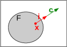
(a) Counterexample candidate.

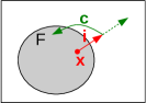
(b) Check.

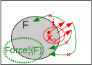
(c) Generalization.

Figure 8: Working principle of SatWin0.

Illustration. Figure 8 illustrates the working principle of SatWin0 graphically. As before, a box represents the set of all states. In Figure 8a, a counterexample candidate is computed in form of a state $\mathbf{x}$ from which some input $\mathbf{i}$ and some control value $\mathbf{c}$ lead from $F$ to $\neg F$. This corresponds to the SAT solver call in Line 5. In case of satisfiability, the next step is to check if some alternative $\mathbf{c}$ leads back to $F$ (for the same $\mathbf{x}$ and $\mathbf{i}$). This is illustrated in Figure 8b and corresponds to the SAT solver call in Line 9. In case of satisfiability, $U$ is refined in order not to get the same counterexample candidate again (Line 15), and the algorithm proceeds by computing the next counterexample candidate as shown in Figure 8a. In case of unsatisfiability, $\mathbf{x}$ is indeed a counterexample. Figure 8c illustrates how it is generalized into a larger region $\mathbf{x}_{g}$ for which input $\mathbf{i}$ enforces that the next state is in $\neg F$: it is ensured that, from any state of $\mathbf{x}_{g}$, with input $\mathbf{i}$, no $\mathbf{c}$ can exist such that the next state is in $F$ again. This is a sufficient but not a necessary condition for $F\wedge\mathbf{x}_{g}$ not to intersect with $\mathsf{Force}^{s}_{1}(F)$. This generalization corresponds to the computation of the unsatisfiable core in Line 11 of SatWin0. Finally, $\mathbf{x}_{g}$ is removed from $F$ and the procedure continues with Figure 8a.

Discussion. In contrast to QbfWin (Algorithm 6), SatWin0 potentially requires far more solver calls. This has two reasons. First, many refinements of $U$ may be necessary until a genuine counterexample is found. In contrast, QbfWin computes a counterexample with one single solver call. Second, the counterexample generalization in SatWin0 is weaker and may thus drop fewer literals. This can increase the number of counterexamples that needs to be computed. The advantage of SatWin0 is that all satisfiability checks are propositional and, thus, potentially less expensive.

The main purpose of discussing SatWin0 from Algorithm 8 was to prepare for a more advanced version, which will be presented in the next section. Hence, we will not elaborate on implementation aspects or formal correctness arguments for Algorithm 8, but only do this for the advanced version, which is presented in the next section.

3.2.2 Advanced Algorithm

The basic algorithm from the previous section has two main weaknesses. First, a reset of $U$ needs to be done upon every update of $F$. After such a reset, a lot of iterations may be necessary until $U$ is again restrictive enough for Line 5 to produce a counterexample. Second, incremental solving is difficult in Line 5 due to the negation of $F$: clauses are added to $F$, but this makes $\neg F$ weaker, which can only be expressed by (also) removing clauses from the CNF representation of $\neg F$. The procedure SatWin1 in Algorithm 9 resolves these weaknesses. The differences to SatWin0 are marked in blue.

Algorithm 9 SatWin1: Advanced SAT solver based CNF learning algorithm for computing the winning region.

1:procedure SatWin1$\left((\overline{x},\overline{i},\overline{c},I,T,P)\right)$, returns: The winning region $W(\overline{x})$ in CNF or $\mathsf{false}$

2:   if $\textsc{PropSat}\bigl{(}I(\overline{x})\wedge\neg P(\overline{x})\bigr{)}$ then return $\mathsf{false}$

3:   $F(\overline{x}):=P(\overline{x})$, $U(\overline{x},\overline{i}):=\mathsf{true}$, $G(\overline{x}):=F(\overline{x})$, $\textsf{precise}:=\mathsf{true}$

4:   while $\mathsf{true}$ do

5:      $(\mathsf{sat},\mathbf{x},\mathbf{i}):=\textsc{PropSatModel}\bigl{(}F(\overline{x})\wedge U(\overline{x},\overline{i})\wedge T(\overline{x},\overline{i},\overline{c},\overline{x}^{\prime})\wedge\neg{\color[rgb]{0,0,1}G}(\overline{x}^{\prime})\bigr{)}$

6:      if $\neg\mathsf{sat}$ then

7:         if precise then return $F(\overline{x})$

8:         $U(\overline{x},\overline{i}):=\mathsf{true}$, $G(\overline{x}):=F(\overline{x})$, $\textsf{precise}:=\mathsf{true}$

9:      else

10:         $(\mathsf{sat},\mathbf{c}):=\textsc{PropSatModel}\bigl{(}F(\overline{x})\wedge\mathbf{x}\wedge\mathbf{i}\wedge T(\overline{x},\overline{i},\overline{c},\overline{x}^{\prime})\wedge F(\overline{x}^{\prime})\bigr{)}$

11:         if $\neg\mathsf{sat}$ then

12:            $\mathbf{x}_{g}:=\textsc{PropMinUnsatCore}\bigl{(}\mathbf{x},F(\overline{x})\wedge\mathbf{i}\wedge T(\overline{x},\overline{i},\overline{c},\overline{x}^{\prime})\wedge F(\overline{x}^{\prime})\bigr{)}$

13:            if $\textsc{PropSat}\bigl{(}\mathbf{x}_{g}\wedge I(\overline{x})\bigr{)}$ then return $\mathsf{false}$

14:            $F(\overline{x}):=F(\overline{x})\wedge\neg\mathbf{x}_{g}$, $\textsf{precise}:=\mathsf{false}$

15:         else

16:            $U:=U\wedge\neg\textsc{PropMinUnsatCore}\bigl{(}\mathbf{x}\wedge\mathbf{i},\mathbf{c}\wedge F(\overline{x})\wedge U(\overline{x},\overline{i})\wedge T(\overline{x},\overline{i},\overline{c},\overline{x}^{\prime})\wedge\neg{\color[rgb]{0,0,1}G}(\overline{x}^{\prime})\bigr{)}$                   

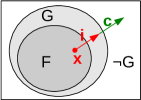
Figure 9: Counterexample candidate in SatWin1.

Lazy updates of $F$. The formula $G(\overline{x})$ is a copy of $F(\overline{x})$ that is updated only lazily with newly discovered clauses. Consequently, $F\rightarrow G$ holds at any time, i.e., $G$ always represents a superset of the states in $F$. The Boolean flag precise is $\mathsf{true}$ whenever $G=F$. While SatWin0 computed a transition from $F$ to $\neg F$ in Line 5, SatWin1 computes a transition from $F$ to $\neg G$. This is illustrated in Figure 9. A transition from $F$ to $\neg G$ is also a transition from $F$ to $\neg F$. Thus, in case of satisfiability, nothing changes. However, if no such transition exists, this does not automatically mean that no transition from $F$ to $\neg F$ exists. Therefore, if $G\neq F$, Line 8 sets $G:=F$ and the check is repeated. Only if $G=F$ (indicated by $\textsf{precise}=\mathsf{true}$), the algorithm can conclude that no more counterexample exists and returns $F$ as result.

Updates of $U$. New clauses are only added to $F$ but not to $G$ in Line 14. Thus, after any update of $F$, precise must be set to $\mathsf{false}$. However, $U$ can be kept as it is. The intuitive reason is as follows. If a certain $(\mathbf{x},\mathbf{i})$-pair is not helpful for the environment to enforce a transition from $F$ to $\neg G$, then it will definitely not be helpful to enforce a transition from some smaller set $F\wedge H$ of states into the same region $\neg G$. More formally, we have that

$$\Bigl{(}(\mathbf{x},\mathbf{i})\not\models\forall\overline{c}\operatorname{\mathbin{:}}\exists\overline{x}^{\prime}\operatorname{\mathbin{:}}F(\overline{x})\wedge T(\overline{x},\overline{i},\overline{c},\overline{x}^{\prime})\wedge\neg G(\overline{x}^{\prime})\Bigr{)}\text{ implies }\Bigl{(}(\mathbf{x},\mathbf{i})\not\models\forall\overline{c}\operatorname{\mathbin{:}}\exists\overline{x}^{\prime}\operatorname{\mathbin{:}}F(\overline{x})\wedge H(\overline{x})\wedge T(\overline{x},\overline{i},\overline{c},\overline{x}^{\prime})\wedge\neg G(\overline{x}^{\prime})\Bigr{)}\text{ because}$$

$$\Bigl{(}\forall\overline{c}\operatorname{\mathbin{:}}\exists\overline{x}^{\prime}\operatorname{\mathbin{:}}F(\overline{x})\wedge H(\overline{x})\wedge T(\overline{x},\overline{i},\overline{c},\overline{x}^{\prime})\wedge\neg G(\overline{x}^{\prime})\Bigr{)}\rightarrow\Bigl{(}\forall\overline{c}\operatorname{\mathbin{:}}\exists\overline{x}^{\prime}\operatorname{\mathbin{:}}F(\overline{x})\wedge T(\overline{x},\overline{i},\overline{c},\overline{x}^{\prime})\wedge\neg G(\overline{x}^{\prime})\Bigr{)}.\hskip 91.04881pt$$

Only when $G$ changes in Line 8, $U$ also becomes invalid and needs to be reset to $\mathsf{true}$.

3.2.3 Correctness of the Advanced Algorithm SatWin1

We now work out a formal correctness argument for SatWin1, split into several lemmas to increase readability.

Lemma 7

The SatWin1 procedure in Algorithm 9 always terminates.

Proof 2

Every loop iteration must end with one of the following five events: (1) the loop terminates in Line 7, (2) $U$ is set to $\mathsf{true}$ in Line 8, (3) the loop terminates in Line 13, (4) $F$ shrinks in Line 14, or (5) $U$ shrinks in Line 16. We show that all these events lead to termination or eventual shrinking of $F$: Item (2) cannot happen twice in a row without shrinking $F$ in between: this is prevented by having $\textsf{precise}=\mathsf{true}$. Item (5) cannot happen infinitely often without shrinking $F$ in between because at some point $U$ would reach $\mathsf{false}$, which makes Line 5 return $\textsf{sat}=\mathsf{false}$. In this case, the algorithm either terminates in Line 7, or item (2) occurs, and item (2) cannot occur twice without shrinking $F$ in between. Hence, the loop either terminates or makes some progress towards shrinking $F$. Before $F$ can shrink below $I$, the loop definitely terminates in Line 13.

Lemma 8

SatWin1 enforces the invariant $I(\overline{x})\rightarrow F(\overline{x})\rightarrow P(\overline{x})$.

Proof 3

As for QbfWin (see Theorem 6), $I\rightarrow F$ is enforced by Line 2 and 13; $F\rightarrow P$ is enforced by Line 3 and 14.

Lemma 9

SatWin1 enforces the invariant $W(\overline{x})\rightarrow F(\overline{x})$.

Proof 4

Similar to Theorem 6, this can be proven induction: Initially $F=P$, so $W\rightarrow F$ holds because $W\rightarrow P$. Given that $W\rightarrow F$ holds before an update of $F$ in Line 14, it will also hold after the update because Line 12 ensures that $\mathbf{x}_{g}\wedge F(\overline{x})\wedge\mathbf{i}\wedge T(\overline{x},\overline{i},\overline{c},\overline{x}^{\prime})\wedge F(\overline{x}^{\prime})$ is unsatisfiable. Consequently, we have that $\forall\overline{x},\overline{i},\overline{c},\overline{x}^{\prime}\operatorname{\mathbin{:}}\bigl{(}\mathbf{x}_{g}\wedge F(\overline{x})\wedge\mathbf{i}\bigr{)}\rightarrow\bigl{(}\neg T(\overline{x},\overline{i},\overline{c},\overline{x}^{\prime})\vee\neg F(\overline{x}^{\prime})\bigr{)}.$ Because $T$ is both deterministic and complete ($\overline{x}^{\prime}$ is always uniquely defined by $T$; see Definition 4) we can apply the one-point rule (2) in order to rewrite the implication $\forall\overline{x}^{\prime}\operatorname{\mathbin{:}}T(\overline{x},\overline{i},\overline{c},\overline{x}^{\prime})\rightarrow\neg F(\overline{x}^{\prime})$ to $\exists\overline{x}^{\prime}\operatorname{\mathbin{:}}T(\overline{x},\overline{i},\overline{c},\overline{x}^{\prime})\wedge\neg F(\overline{x}^{\prime})$. This gives $\forall\overline{x},\overline{i},\overline{c}\operatorname{\mathbin{:}}\exists\overline{x}^{\prime}\operatorname{\mathbin{:}}\bigl{(}\mathbf{x}_{g}\wedge F(\overline{x})\wedge\mathbf{i}\bigr{)}\rightarrow\bigl{(}T(\overline{x},\overline{i},\overline{c},\overline{x}^{\prime})\wedge\neg F(\overline{x}^{\prime})\bigr{)}.$ Using the one point rule (1) on $\overline{i}$, this formula is equivalent to $\forall\overline{x}\operatorname{\mathbin{:}}\exists\overline{i}\operatorname{\mathbin{:}}\forall\overline{c}\operatorname{\mathbin{:}}\exists\overline{x}^{\prime}\operatorname{\mathbin{:}}\mathbf{i}\wedge\bigl{(}\bigl{(}\mathbf{x}_{g}\wedge F(\overline{x})\bigr{)}\rightarrow\bigl{(}T(\overline{x},\overline{i},\overline{c},\overline{x}^{\prime})\wedge\neg F(\overline{x}^{\prime})\bigr{)}\bigr{)}.$ This implies $\forall\overline{x}\operatorname{\mathbin{:}}\exists\overline{i}\operatorname{\mathbin{:}}\forall\overline{c}\operatorname{\mathbin{:}}\exists\overline{x}^{\prime}\operatorname{\mathbin{:}}\bigl{(}\bigl{(}\mathbf{x}_{g}\wedge F(\overline{x})\bigr{)}\rightarrow\bigl{(}T(\overline{x},\overline{i},\overline{c},\overline{x}^{\prime})\wedge\neg F(\overline{x}^{\prime})\bigr{)}\bigr{)}$, which can be written as $\mathbf{x}_{g}\wedge F(\overline{x})\rightarrow\exists\overline{i}\operatorname{\mathbin{:}}\forall\overline{c}\operatorname{\mathbin{:}}\exists\overline{x}^{\prime}\operatorname{\mathbin{:}}T(\overline{x},\overline{i},\overline{c},\overline{x}^{\prime})\wedge\neg F(\overline{x}^{\prime}).$ By substituting the definition of $\mathsf{Force}^{e}_{1}$, we get $\mathbf{x}_{g}\wedge F\rightarrow\mathsf{Force}^{e}_{1}(\neg F)$. Using the induction hypothesis $W\rightarrow F$, which can be written as $\neg F\rightarrow\neg W$, this means that $\mathbf{x}_{g}\wedge F\rightarrow\mathsf{Force}^{e}_{1}(\neg W)$ holds. Thus, only states that cannot be part of $W$ are removed in Line 14. In other words, $F$ cannot shrink below $W$.

The following lemma states that the formula $F(\overline{x})\wedge\neg U(\overline{x},\overline{i})$ can only represent state-input pairs for which the system player can reach $G$ and thus avoid ending up in $\neg G$. In other words, the conjunction with $U$ in the SAT solver call of Line 5 excludes only state-input pairs for which the environment cannot enforce a transition from $F$ to $\neg G$.

Lemma 10

SatWin1 enforces the invariant $\forall\overline{x},\overline{i}\operatorname{\mathbin{:}}\bigl{(}F(\overline{x})\wedge\neg U(\overline{x},\overline{i})\bigr{)}\rightarrow\bigl{(}\exists\overline{c},\overline{x}^{\prime}\operatorname{\mathbin{:}}T(\overline{x},\overline{i},\overline{c},\overline{x}^{\prime})\wedge G(\overline{x}^{\prime})\bigr{)}$.

Proof 5

$U$ is initialized to $\mathsf{true}$, so the invariant holds initially. Line 8 sets $U=\mathsf{true}$ and thus retains the invariant. Line 14 also retains the invariant because $F$ only gets stricter. It remains to be shown that Line 16 retains the invariant. Let $\mathbf{u}$ be the result of PropMinUnsatCore in Line 16. The update $U:=U\wedge\neg\mathbf{u}$ in Line 16 changes the invariant to $\forall\overline{x},\overline{i}\operatorname{\mathbin{:}}\bigl{(}F(\overline{x})\wedge(\neg U(\overline{x},\overline{i})\vee\mathbf{u})\bigr{)}\rightarrow\bigl{(}\exists\overline{c},\overline{x}^{\prime}\operatorname{\mathbin{:}}T(\overline{x},\overline{i},\overline{c},\overline{x}^{\prime})\wedge G(\overline{x}^{\prime})\bigr{)},$ which can be written as $\forall\overline{x},\overline{i}\operatorname{\mathbin{:}}\bigl{(}\bigl{(}F(\overline{x})\wedge\neg U(\overline{x},\overline{i})\bigr{)}\vee\bigl{(}F(\overline{x})\wedge U(\overline{x},\overline{i})\wedge\mathbf{u}\bigr{)}\bigr{)}\rightarrow\bigl{(}\exists\overline{c},\overline{x}^{\prime}\operatorname{\mathbin{:}}T(\overline{x},\overline{i},\overline{c},\overline{x}^{\prime})\wedge G(\overline{x}^{\prime})\bigr{)}.$ In general, a formula $(A\vee B)\rightarrow C$ holds iff $A\rightarrow C$ and $B\rightarrow C$. By induction, we know that $\forall\overline{x},\overline{i}\operatorname{\mathbin{:}}\bigl{(}F(\overline{x})\wedge\neg U(\overline{x},\overline{i})\bigr{)}\rightarrow\bigl{(}\exists\overline{c},\overline{x}^{\prime}\operatorname{\mathbin{:}}T(\overline{x},\overline{i},\overline{c},\overline{x}^{\prime})\wedge G(\overline{x}^{\prime})\bigr{)}$ holds. What remains to be shown is that $\forall\overline{x},\overline{i}\operatorname{\mathbin{:}}\bigl{(}F(\overline{x})\wedge U(\overline{x},\overline{i})\wedge\mathbf{u}\bigr{)}\rightarrow\bigl{(}\exists\overline{c},\overline{x}^{\prime}\operatorname{\mathbin{:}}T(\overline{x},\overline{i},\overline{c},\overline{x}^{\prime})\wedge G(\overline{x}^{\prime})\bigr{)}$ also holds. Since $\mathbf{u}\wedge\mathbf{c}\wedge F(\overline{x})\wedge U(\overline{x},\overline{i})\wedge T(\overline{x},\overline{i},\overline{c},\overline{x}^{\prime})\wedge\neg G(\overline{x}^{\prime})$ is unsatisfiable (enforced by Line 16), we have that $\forall\overline{x},\overline{i}\operatorname{\mathbin{:}}\bigl{(}F(\overline{x})\wedge U(\overline{x},\overline{i})\wedge\mathbf{u}\bigr{)}\rightarrow\bigl{(}\forall\overline{c},\overline{x}^{\prime}\operatorname{\mathbin{:}}\neg\mathbf{c}\vee\neg T(\overline{x},\overline{i},\overline{c},\overline{x}^{\prime})\vee G(\overline{x}^{\prime})\bigr{)}.$ By applying the one-point rule (Eq. (1) for $\overline{c}$ and Eq. (2) for $\overline{x}^{\prime}$), this can also be written as $\forall\overline{x},\overline{i}\operatorname{\mathbin{:}}\bigl{(}F(\overline{x})\wedge U(\overline{x},\overline{i})\wedge\mathbf{u}\bigr{)}\rightarrow\bigl{(}\exists\overline{c},\overline{x}^{\prime}\operatorname{\mathbin{:}}\mathbf{c}\wedge T(\overline{x},\overline{i},\overline{c},\overline{x}^{\prime})\wedge G(\overline{x}^{\prime})\bigr{)}.$ This formula obviously implies $\forall\overline{x},\overline{i}\operatorname{\mathbin{:}}\bigl{(}F(\overline{x})\wedge U(\overline{x},\overline{i})\wedge\mathbf{u}\bigr{)}\rightarrow\bigl{(}\exists\overline{c},\overline{x}\operatorname{\mathbin{:}}T(\overline{x},\overline{i},\overline{c},\overline{x}^{\prime})\wedge G(\overline{x}^{\prime})\bigr{)},$ which was to be shown for Line 16 to preserve the invariant.

Lemma 11

If SatWin1 reaches Line 7, $F(\overline{x})=W(\overline{x})$ holds at that point.

Proof 6

Line 7 is only reached when $G=F$ (otherwise precise is $\mathsf{false}$) and $F(\overline{x})\wedge U(\overline{x},\overline{i})\wedge T(\overline{x},\overline{i},\overline{c},\overline{x}^{\prime})\wedge\neg G(\overline{x}^{\prime})$ is unsatisfiable, which means that $\forall\overline{x},\overline{i}\operatorname{\mathbin{:}}\bigl{(}F(\overline{x})\wedge U(\overline{x},\overline{i})\bigr{)}\rightarrow\bigl{(}\forall\overline{c}\operatorname{\mathbin{:}}\forall\overline{x}^{\prime}\operatorname{\mathbin{:}}\neg T(\overline{x},\overline{i},\overline{c},\overline{x}^{\prime})\vee F(\overline{x}^{\prime})\bigr{)}$ holds. By applying the one-point rule (2), this can also be written as $\forall\overline{x},\overline{i}\operatorname{\mathbin{:}}\bigl{(}F(\overline{x})\wedge U(\overline{x},\overline{i})\bigr{)}\rightarrow\bigl{(}\forall\overline{c}\operatorname{\mathbin{:}}\exists\overline{x}^{\prime}\operatorname{\mathbin{:}}T(\overline{x},\overline{i},\overline{c},\overline{x}^{\prime})\wedge F(\overline{x}^{\prime})\bigr{)}.$ In turn, this implies $\forall\overline{x},\overline{i}\operatorname{\mathbin{:}}\bigl{(}F(\overline{x})\wedge U(\overline{x},\overline{i})\bigr{)}\rightarrow\bigl{(}\exists\overline{c}\operatorname{\mathbin{:}}\exists\overline{x}^{\prime}\operatorname{\mathbin{:}}T(\overline{x},\overline{i},\overline{c},\overline{x}^{\prime})\wedge F(\overline{x}^{\prime})\bigr{)}.$ From Lemma 10, we know that $\forall\overline{x},\overline{i}\operatorname{\mathbin{:}}\bigl{(}F(\overline{x})\wedge\neg U(\overline{x},\overline{i})\bigr{)}\rightarrow\bigl{(}\exists\overline{c}\operatorname{\mathbin{:}}\exists\overline{x}^{\prime}\operatorname{\mathbin{:}}T(\overline{x},\overline{i},\overline{c},\overline{x}^{\prime})\wedge F(\overline{x}^{\prime})\bigr{)}.$ Since $A\wedge B\rightarrow C$ and $A\wedge\neg B\rightarrow C$ together imply $A\rightarrow C$, we can conclude that $\forall\overline{x}\operatorname{\mathbin{:}}F(\overline{x})\rightarrow\forall\overline{i}\operatorname{\mathbin{:}}\exists\overline{c},\overline{x}^{\prime}\operatorname{\mathbin{:}}T(\overline{x},\overline{i},\overline{c},\overline{x}^{\prime})\wedge F(\overline{x}^{\prime})$ must hold in Line 7. This means that the returned $F$ satisfies $F\rightarrow\mathsf{Force}^{s}_{1}(F)$. From $W\rightarrow F\rightarrow P$ (Lemma 9 and 8), it follows that $F=W$. The reason is that $W$ is the set of all states from which the system player can enforce the specification, i.e., no proper superset $H$ of $W$ can satisfy $H\rightarrow P$ and $H\rightarrow\mathsf{Force}^{s}_{1}(H)$.

Theorem 12

The SatWin1 procedure in Algorithm 9 returns the winning region $W(\overline{x})$ of a given safety specification $\mathcal{S}$, or $\mathsf{false}$ if the specification is unrealizable.

Proof 7

Unrealizability: If $\mathcal{S}$ is unrealizable, $I\not\rightarrow W$. SatWin1 terminates (Lemma 7), but cannot terminate in Line 7 because $F=W$ (Lemma 11) contradicts with $I\not\rightarrow W$ (unrealizability) and $I\rightarrow F$ (Lemma 8). Hence, in case of unrealizability, SatWin1 must terminate in Line 2 or 13 returning $\mathsf{false}$.

Realizability: SatWin1 can only return $\mathsf{false}$ in Line 2 or 13 if $F$ is about to be updated such that $I\not\rightarrow F$. From $I\rightarrow W$ (realizability) and $W\rightarrow F$ (Lemma 9), it follows that $I\rightarrow F$, so this can never happen. Yet, Lemma 7 says that SatWin1 terminates, so it must reach Line 7 eventually. By Lemma 11, this will return the winning region.

3.2.4 Efficient Implementation

This section discusses some important aspects of implementing SatWin1 efficiently.

Incremental solving. We propose to use three SAT solver instances incrementally. The first one will be called solverC and stores $F(\overline{x})\wedge U(\overline{x},\overline{i})\wedge T(\overline{x},\overline{i},\overline{c},\overline{x}^{\prime})\wedge\neg G(\overline{x}^{\prime})$. solverC is used in Line 5 and Line 16, where the conjunction with $\mathbf{c}$ is realized with temporarily asserted assumption literals. Whenever Line 8 is reached, solverC is reset with the new CNF encoding of $\neg G(\overline{x}^{\prime})=\neg F(\overline{x}^{\prime})$. Otherwise, clauses are only added to $F$ or $U$. The second solver instance, called solverG, stores $F(\overline{x})\wedge T(\overline{x},\overline{i},\overline{c},\overline{x}^{\prime})\wedge F(\overline{x}^{\prime})$ and is used for Line 10 and Line 12. Clauses are only added to $F$, so solverG does not have to be reset at all. The conjunctions with $\mathbf{i}$ and $\mathbf{x}$, which change from iteration to iteration, are again realized by setting assumption literals. The lines 10 and 12 are actually combined into one SAT solver call that returns either a satisfying assignment $\mathbf{c}$ or an unsatisfiable core. The third solver instance stores $I(\overline{x})$ and is used in Line 13. The conjunction with $\mathbf{x}_{g}$ is again realized with assumption literals.

CNF compression. Whenever solverC is reset with the current CNF encoding of $\neg G(\overline{x}^{\prime})=\neg F(\overline{x}^{\prime})$ in Line 8, we call CompressCnf from Algorithm 7 (with literal dropping disabled) in order to reduce the size of $F$ beforehand. This results in a more compact CNF encoding of $\neg G(\overline{x}^{\prime})$ when using the method of Plaisted and Greenbaum [31].

Resets of solverG. By default, we only add clauses to solverG. However, after some iterations, many of the $F$-clauses added to solverG can become redundant because they can be implied by (a combination of) other clauses that have been added later. To prevent the clause database of solverG from growing unreasonably, we also reset solverG with the compressed $F$ from time to time. As a heuristic, we track the number of $F$-clauses that have been added to solverG so far, and compute the difference to the number of clauses in the compressed $F$. If this difference exceeds a certain limit, solverG is reset. This can give a moderate speedup for certain SAT solvers and benchmarks.

3.3 Partial Quantifier Expansion

The procedure QbfWin in Algorithm 6 uses quantified formulas to compute counterexamples witnessing that $F\neq W$ and to generalize these counterexamples. In contrast, the procedure SatWin1 in Algorithm 9 avoids the universal quantifiers. This results in less expensive solver calls, but comes at the price of requiring more iterations of the outer loop. In this section, we will discuss a hybrid approach which quantifies universally over some (but not necessarily all) variables. The universal quantification is then eliminated by applying universal expansion so that the resulting formulas can be solved with a plain SAT solver. The hope is to find a sweet spot where the reduction in the number of iterations is more significant than the additional costs per solver call.

3.3.1 Quantifier Expansion in Counterexample Computation

The procedure QbfWin in Algorithm 6 computes counterexamples to $F=W$ by solving the quantified formula $\exists\overline{x},\overline{i}\operatorname{\mathbin{:}}\forall\overline{c}\operatorname{\mathbin{:}}\exists\overline{x}^{\prime}\operatorname{\mathbin{:}}F(\overline{x})\wedge T(\overline{x},\overline{i},\overline{c},\overline{x}^{\prime})\wedge\neg F(\overline{x}^{\prime}).$ In contrast, the SatWin1 procedure from Algorithm 9 avoids the universal quantification of the variables $\overline{c}$ by solving the formula $\exists\overline{x},\overline{i}\operatorname{\mathbin{:}}\exists\overline{c}\operatorname{\mathbin{:}}\exists\overline{x}^{\prime}\operatorname{\mathbin{:}}F(\overline{x})\wedge U(\overline{x},\overline{i})\wedge T(\overline{x},\overline{i},\overline{c},\overline{x}^{\prime})\wedge\neg G(\overline{x}^{\prime}),$ where $G$ is just a copy of $F$ that may not be fully up to date. The latter formula does not necessarily yield a counterexample, but only a candidate. If the candidate turns out to be spurious, it is excluded by refining $U$. This approach can be seen as a “lazy elimination” of the universal quantification over $\overline{c}$ via $U$. The disadvantage is that many refinements of $U$ may be necessary before the first genuine counterexample is found. One alternative would be to eliminate $\forall\overline{c}$ in $\exists\overline{x},\overline{i}\operatorname{\mathbin{:}}\forall\overline{c}\operatorname{\mathbin{:}}\exists\overline{x}^{\prime}\operatorname{\mathbin{:}}F(\overline{x})\wedge T(\overline{x},\overline{i},\overline{c},\overline{x}^{\prime})\wedge\neg G(\overline{x}^{\prime})$ eagerly by performing universal expansion as explained in Section 2.1.2. Yet, this may blow up the formula size by a factor of $2^{|\overline{c}|}$ and may thus be infeasible. Another alternative is to partition the variables of $\overline{c}$ into two subsets $\overline{c}_{1}$ and $\overline{c}_{2}$ and solve

$$\exists\overline{x},\overline{i}\operatorname{\mathbin{:}}\exists\overline{c}_{1}\operatorname{\mathbin{:}}\forall\overline{c}_{2}\operatorname{\mathbin{:}}\exists\overline{x}^{\prime}\operatorname{\mathbin{:}}F(\overline{x})\wedge U(\overline{x},\overline{i})\wedge T(\overline{x},\overline{i},\overline{c},\overline{x}^{\prime})\wedge\neg G(\overline{x}^{\prime})$$

using a SAT solver by expanding only over the variables in $\overline{c}_{2}$. By adjusting the relative size of $\overline{c}_{2}$, different trade-offs between decreasing the number of refinements to $U$ and increasing the costs per solver call can be achieved.

3.3.2 Quantifier Expansion in Counterexample Generalization

The idea is similar to that of the previous subsection. QbfWin eliminates literals from a counterexample $\mathbf{x}$ as long as $\exists\overline{x}\operatorname{\mathbin{:}}\forall\overline{i}\operatorname{\mathbin{:}}\exists\overline{c},\overline{x}^{\prime}\operatorname{\mathbin{:}}\mathbf{x}_{g}\wedge F(\overline{x})\wedge T(\overline{x},\overline{i},\overline{c},\overline{x}^{\prime})\wedge F(\overline{x}^{\prime})$ is unsatisfiable. In contrast, SatWin1 avoids the universal quantification over $\overline{i}$ by ensuring that $\exists\overline{x}\operatorname{\mathbin{:}}\exists\overline{i}\operatorname{\mathbin{:}}\exists\overline{c},\overline{x}^{\prime}\operatorname{\mathbin{:}}\mathbf{x}\wedge\mathbf{i}\wedge F(\overline{x})\wedge T(\overline{x},\overline{i},\overline{c},\overline{x}^{\prime})\wedge F(\overline{x}^{\prime})$ is unsatisfiable for some concrete $\mathbf{i}$. The latter check is potentially cheaper, but may result in fewer literals being eliminated from $\mathbf{x}$. This means that the refinement of $F$ is less substantial, so more iterations may be needed. By partitioning the variables $\overline{i}$ into $\overline{i}_{1}$ and $\overline{i}_{2}$ and checking $\exists\overline{x}\operatorname{\mathbin{:}}\exists\overline{i}\operatorname{\mathbin{:}}\mathbf{x}\wedge\mathbf{i}\wedge F(\overline{x})\wedge\forall\overline{i}_{2}\operatorname{\mathbin{:}}\exists\overline{c},\overline{x}^{\prime}\operatorname{\mathbin{:}}T(\overline{x},\overline{i},\overline{c},\overline{x}^{\prime})\wedge F(\overline{x}^{\prime})$ for unsatisfiability, different trade-offs between the generalization procedure of QbfWin and that of SatWin1 can be realized.

3.3.3 Efficient Implementation

Universal expansion needs to be implemented carefully in order to avoid an unnecessary blow-up of the formula size, and to keep the time for the expansion low. Our experience showed that even small inefficiencies can cost orders of magnitude in both metrics.

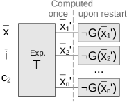
Figure 10: Universal expansion for counterexample computation.

Expansion for counterexample computation. Since $F(\overline{x})$ and $U(\overline{x},\overline{i})$ are independent of $\overline{c}$ and $\overline{x}^{\prime}$, we apply universal expansion to $\forall\overline{c}_{2}\operatorname{\mathbin{:}}\exists\overline{x}^{\prime}\operatorname{\mathbin{:}}T(\overline{x},\overline{i},\overline{c},\overline{x}^{\prime})\wedge\neg G(\overline{x}^{\prime})$ and conjoin $F(\overline{x})\wedge U(\overline{x},\overline{i})$ afterwards. The transition relation $T$ is always fixed, but $\neg G(\overline{x}^{\prime})$ changes upon every restart of solverC in Line 8 of SatWin1. Hence, we expand $T$ only once and store the resulting renamings $\overline{x}^{\prime}_{1},\ldots\overline{x}^{\prime}_{n}$ of $\overline{x}^{\prime}$. A copy of $\neg G(\overline{x}^{\prime})$ is then added for each renaming $\overline{x}^{\prime}_{i}$ when solverC is initialized or restarted. This is illustrated in Figure 10.

Expansion of $T$. In our implementation, $T$ is originally given as a circuit of AND-gates (where inputs can be negated). We perform the expansion of $T$ directly on this circuit and only encode the result into CNF. This facilitates efficient constant propagation and other simplifications. When expanding a certain $c\in\overline{c}_{2}$, we only copy those AND-gates that have $c$ in their fan-in cone. Whenever the copy of some AND-gate has the same inputs as some existing AND-gate, the existing gate is reused. Finally, the tool ABC [67] is called to simplify the expanded circuit. This involves fraiging, which ensures that no two nodes in the circuit can represent the same function over the inputs. Hence, equivalent (copies of) next-state signals will be represented by the same variable, which enables a more substantial simplification of the $\neg G(\overline{x}^{\prime})$ copies (see Figure 10). Finally, duplicate renamings of the next-state variables are removed. Since $T$ is expanded only once, these simplifications can be afforded.

Expansion of $\neg G(\overline{x}^{\prime})$. First, we perform an even more aggressive compression of $G(\overline{x}^{\prime})$ than done by CompressCnf in Algorithm 7. CompressCnf removes a clause $c$ from a CNF $A$ if $\bigl{(}A\setminus\{c\}\bigr{)}\rightarrow c$, i.e., if the clause is implied by other clauses of $A$ already. We now remove a clause $c$ from $G(\overline{x}^{\prime})$ if $\bigl{(}F(\overline{x})\wedge T(\overline{x},\overline{i},\overline{c},\overline{x}^{\prime})\wedge\bigl{(}G(\overline{x}^{\prime})\setminus\{c\}\bigr{)}\bigr{)}\rightarrow c.$ Hence, the compressed $G(\overline{x}^{\prime})$ will only be equivalent to the original $G(\overline{x}^{\prime})$ if the current state is in $F$, but this is asserted in all SAT solver calls of SatWin1 anyway. For every renaming $\overline{x}^{\prime}_{i}$ of $\overline{x}^{\prime}$ that has been created during the expansion of $T$, we then perform the following steps: First, $G(\overline{x}^{\prime}_{i})$ is computed by applying the renaming. Second, $G(\overline{x}^{\prime}_{i})$ is simplified by removing tautological clauses and performing unit clause propagation. Finally, $G(\overline{x}^{\prime}_{i})$ is negated, while auxiliary variables that have already been introduced during the negation of other copies of $G(\overline{x}^{\prime})$ are reused. All these measures contribute towards reducing the size of the expansion of $\neg G(\overline{x}^{\prime})$.

Expansion in counterexample generalization. This is easier, since no negation of a CNF is involved. Again, $T$ is expanded and the resulting renamings $\overline{x}^{\prime}_{1},\ldots\overline{x}^{\prime}_{n}$ of $\overline{x}^{\prime}$ are stored. Whenever a clause $\neg\mathbf{x}_{g}$ is added to $F$, we do not only add it to solverG but also add all the renamed next-state copies of the clause to solverG.

Configuration. In our experiments, choosing low numbers for $|\overline{c}_{2}|$ only slowed down the SatWin1 procedure compared to $|\overline{c}_{2}|=0$. High numbers for $|\overline{c}_{2}|$ did bring a speedup, though, with the best results achieved for $\overline{c}_{2}=\overline{c}$. Furthermore, we observed that an explosion of the formula size can be avoided in most cases by our careful implementation of the formula expansion. Hence, by default, we expand over all variables in $\overline{c}$ and only fall back to $\overline{c}_{2}=\emptyset$ if some memory limit is exceeded. For counterexample generalization, a speedup could only be achieved with low numbers of $|\overline{i}_{2}|$. Hence, by default, we only expand one input signal. As a heuristic, we choose the signal that causes the least number of gates to be copied when expanding the transition relation.

Discussion. Our optimization of partial quantifier expansion can be used to realize different trade-offs between the number of SAT solver calls and their costs in Algorithm 9. We hoped to find a sweet spot between these two cost factors at low expansion rates, but our experiments suggest high rates at least for counterexample computation. While the basic idea of quantifier expansion is simple, such high expansion rates require a careful implementation, like the one discussed in this section, in order not to waste computational resources.

3.4 Reachability Optimizations

In this section, we present optimizations that exploit (un)reachability information when computing a winning region with query learning. The optimizations can be applied to QbfWin (Algorithm 6) and to SatWin1 (Algorithm 9), both with and without partial quantifier elimination. However, to simplify the presentation, we only explain the optimizations for the case of QbfWin in detail. The application to SatWin1 works in exactly the same way.

3.4.1 Optimization RG: Reachability for Counterexample Generalization

Recall that a counterexample $\mathbf{x}\models F\wedge\mathsf{Force}^{e}_{1}(\neg F)$ in QbfWin is a state that is part of the current over-approximation $F$ of the winning region, but this state cannot be part of the final winning region. The state is represented by a minterm $\mathbf{x}$ over the state variables $\overline{x}$. QbfWin generalizes $\mathbf{x}$ into a larger state region $\mathbf{x}_{g}$ by eliminating literals as long as $F\wedge\mathbf{x}_{g}\rightarrow\mathsf{Force}^{e}_{1}(\neg F)$ holds, i.e., as long as $F\wedge\mathbf{x}_{g}\wedge\mathsf{Force}^{s}_{1}(F)$ is unsatisfiable. The reason is that any state $\mathbf{x}_{a}\models F\wedge\mathbf{x}_{g}\wedge\mathsf{Force}^{s}_{1}(F)$ could potentially be part of the winning region, and thus must not be removed from $F$. Yet, as an optimization, we can still remove such a state $\mathbf{x}_{a}$, as long as it is guaranteed that $\mathbf{x}_{a}$ is unreachable from the initial states. Using this insight, we can eliminate literals in a counterexample $\mathbf{x}$ as long as $R\wedge F\wedge\mathbf{x}_{g}\rightarrow\mathsf{Force}^{e}_{1}(\neg F)$, where $R(\overline{x})$ is an over-approximation of the reachable states in $\mathcal{S}$. In QbfWin, this can be realized by conjoining $R$ to the QBF that is checked in Line 8. This may result in more literals being eliminated during the generalization, which means that $F$ is pruned more extensively. Ultimately, this can reduce the number of iterations in QbfWin.

Computing reachable states. The states that are reachable from the initial states in a specification $\mathcal{S}$ can be defined inductively as follows: All states in $I(\overline{x})$ are reachable. If a state $\mathbf{x}$ is reachable, then all states $\mathbf{x}^{\prime}\models\exists\overline{x},\overline{i},\overline{c}\operatorname{\mathbin{:}}\mathbf{x}\wedge T(\overline{x},\overline{i},\overline{c},\overline{x}^{\prime})$ are also reachable. In the synthesis setting, this definition can even be refined. Any over-approximation $F$ of the winning region is itself an over-approximation of the reachable states, not necessarily in the specification $\mathcal{S}$, but definitely in the final implementation. The reason is that no realization of $\mathcal{S}$ must ever leave the winning region $W$, and thus also not $F$. This insight can be used to compute a tighter set of reachable states by considering only transitions that remain in $F$. In principle, the set of reachable states can easily be computed using a simple fixed-point algorithm. However, we consider this to be too expensive, and instead work with over-approximations of the reachable states. Such over-approximations are also useful in formal verification, and many methods to compute them exist [68].

Our approach. We avoid computing an over-approximation of the reachable states explicitly. Instead, we use an idea that is inspired by the model checking algorithm IC3 [24]: Let $R(\overline{x})$ be an over-approximation of the reachable states. By induction, we know that a state $\mathbf{x}$ is definitely unreachable if $I(\overline{x})\rightarrow\neg\mathbf{x}$ and $\neg\mathbf{x}\wedge R(\overline{x})\wedge T(\overline{x},\overline{i},\overline{c},\overline{x}^{\prime})\rightarrow\neg\mathbf{x}^{\prime}$. The formula says that if the current state is reachable but different from $\mathbf{x}$, then the next state cannot be $\mathbf{x}$ either. Hence, if $\mathbf{x}$ is not an initial state, then $\mathbf{x}$ can never be visited. The same reasoning applies if $\mathbf{x}$ is an incomplete cube (or any other formula) representing a set of states. In IC3, $\neg\mathbf{x}$ is said to be inductive relative to the current knowledge $R$ about the reachable states. It can thus be used to refine $R$.

In our synthesis setting, we take the current over-approximation $F$ as an over-approximation of the reachable states. When generalizing a counterexample $\mathbf{x}$, literals cannot only be eliminated if $F\wedge\mathbf{x}_{g}\rightarrow\mathsf{Force}^{e}_{1}(\neg F)$ is preserved, but also if $\neg\mathbf{x}_{g}$ is inductive relative to $F$. The two criteria can be combined by requiring that

$$\exists{\color[rgb]{0,0,1}\overline{x}^{*},\overline{i}^{*},\overline{c}^{*},}\overline{x}\operatorname{\mathbin{:}}\forall\overline{i}\operatorname{\mathbin{:}}\exists\overline{c},\overline{x}^{\prime}\operatorname{\mathbin{:}}{\color[rgb]{0,0,1}\bigl{(}I(\overline{x})\vee F(\overline{x}^{*})\wedge\neg\mathbf{x}_{g}^{*}\wedge T(\overline{x}^{*},\overline{i}^{*},\overline{c}^{*},\overline{x})\bigr{)}\,\wedge\,}\mathbf{x}_{g}\wedge F(\overline{x})\wedge T(\overline{x},\overline{i},\overline{c},\overline{x}^{\prime})\wedge F(\overline{x}^{\prime})$$ (3)

is unsatisfiable. Only the parts of the formula that are marked in blue are new. The variables $\overline{x}^{*}$, $\overline{i}^{*}$ and $\overline{c}^{*}$ are previous-state copies of $\overline{x}$, $\overline{i}$ and $\overline{c}$, respectively. The original version of the formula was $\mathsf{true}$ if some state $\mathbf{x}_{a}\models F\wedge\mathbf{x}_{g}\wedge\mathsf{Force}^{s}_{1}(F)$ exists. The improved formula also requires that $\mathbf{x}_{a}$ is either an initial state, or has a predecessor $\mathbf{x}_{b}$ in $F\wedge\neg\mathbf{x}_{g}$. This is illustrated in the figure on the right. If neither of these two criteria holds, then we know that $I(\overline{x})\rightarrow\neg\mathbf{x}_{a}$ and $\neg\mathbf{x}_{a}\wedge F(\overline{x})\wedge\mathbf{x}_{g}\wedge T(\overline{x},\overline{i},\overline{c},\overline{x}^{\prime})\rightarrow\neg\mathbf{x}_{a}^{\prime}$. This means that $\neg\mathbf{x}_{a}$ is inductive relative to $F\wedge\neg\mathbf{x}_{g}$, so $\mathbf{x}_{a}$ is unreachable and can thus be removed even if it could potentially be part of the winning region. Note that we do not require inductiveness relative to $F$ but rather relative to $F\wedge\neg\mathbf{x}_{g}$. The intuitive reason is that $F$ will be updated to $F\wedge\neg\mathbf{x}_{g}$, so a predecessor $\mathbf{x}_{b}$ in $F\wedge\mathbf{x}_{g}$ does not count. The following theorem states that this procedure cannot prune $F$ too much.

Theorem 13

For a realizable specification $\mathcal{S}$, if Equation (3) is unsatisfiable, then $F\wedge\mathbf{x}_{g}$ cannot contain a state $\mathbf{x}_{a}$ from which (a) the system player can enforce that $F$ is visited in one step, and (b) which is reachable in some implementation of $\mathcal{S}$.

Proof. By contradiction, assume that there exists such as state $\mathbf{x}_{a}$. Any implementation of $\mathcal{S}$ must only visit states in $W$. Hence, for $\mathbf{x}_{a}$ to be reachable in an implementation, there must exist a play $\mathbf{x}_{0},\ldots,\mathbf{x}_{n},\ldots$ of the game $\mathcal{S}$ such that

• $\mathbf{x}_{0}\models I$ (the play starts in the initial states),

• $\mathbf{x}_{n}=\mathbf{x}_{a}$ (the play reaches $\mathbf{x}_{a}$ at some step $n$),

• $n\geq 1$ (that is, $\mathbf{x}_{a}$ cannot be initial because this would satisfy Equation (3)), and

• $\mathbf{x}_{j}\models W$ for all $0\leq j\leq n$ (all states in the play are in the winning region and thus potentially reachable).

Such a play is illustrated on the right. Since $\mathbf{x}_{a}\models F\wedge\mathbf{x}_{g}$, there must exist a smallest $k\leq n$ such that $\mathbf{x}_{j}\models F\wedge\mathbf{x}_{g}$ for all $k\leq j\leq n$. Now, $\mathbf{x}_{k}$ is either initial or has a predecessor $\mathbf{x}_{k-1}$ in $F\wedge\neg\mathbf{x}_{g}$ (because $\mathbf{x}_{k-1}\models W,W\rightarrow F$, and $\mathbf{x}_{k-1}\not\models F\wedge\mathbf{x}_{g}$). Thus, $\mathbf{x}_{k}$ satisfies the new (blue) part of Equation (3). Since Equation (3) is unsatisfiable, the system player cannot enforce that the play traverses from $\mathbf{x}_{k}$ to $F$. Hence, $\mathbf{x}_{k}$ cannot be part of $W$. This contradiction means that such a path of reachable states ending in $\mathbf{x}_{a}$ cannot exist if Equation (3) is unsatisfiable.

Theorem 13 only considers the case of a realizable specification. In case of unrealizability, the correctness argument is even simpler: Optimization RG cannot make QbfWin identify an unrealizable specification as realizable because the additional conjuncts in Equation (3) can only have the effect that more states are removed from $F$, thus $F$ can only shrink below $I$ faster. Another important remark is that QbfWin no longer computes the winning region when optimization RG is enabled, but only a winning area according to Definition 5. The reason is that states of $W$ may be missing in $F$ if they are unreachable.

3.4.2 Optimization RC: Reachability for Counterexample Computation

Similar to improving the generalization of counterexamples using unreachability information, we can also restrict their computation to potentially reachable states. In addition to $\mathbf{x}\models F\wedge\mathsf{Force}^{e}_{1}(\neg F)$, we require that the counterexample $\mathbf{x}$ is either an initial state, or has a predecessor in $F$ that is different from $\mathbf{x}$. If neither of these two conditions is satisfied, then $\mathbf{x}$ can only be unreachable and, thus, does not have to be removed from $F$.

Realization. In QbfWin, these additional constraints can be imposed by modifying the QBF query in Line 4 to

$$\textsc{QbfSatModel}\bigl{(}\exists{\color[rgb]{0,0,1}\overline{x}^{*},\overline{i}^{*},\overline{c}^{*},}\overline{x},\overline{i}\operatorname{\mathbin{:}}\forall\overline{c}\operatorname{\mathbin{:}}\exists\overline{x}^{\prime}\operatorname{\mathbin{:}}\\ {\color[rgb]{0,0,1}\bigl{(}I(\overline{x})\vee\overline{x}^{*}\neq\overline{x}\wedge F(\overline{x}^{*})\wedge T(\overline{x}^{*},\overline{i}^{*},\overline{c}^{*},\overline{x})\bigr{)}\wedge}F(\overline{x})\wedge T(\overline{x},\overline{i},\overline{c},\overline{x}^{\prime})\wedge\neg F(\overline{x}^{\prime})\bigr{)}.$$ (4)

As before, the new parts are marked in blue, and $\overline{x}^{*}$, $\overline{i}^{*}$, and $\overline{c}^{*}$ are the previous-state copies of $\overline{x}$, $\overline{i}$, and $\overline{c}$, respectively. The expression $\overline{x}^{*}\neq\overline{x}$ requires that at least one state variable $x\in\overline{x}$ has a different value than its previous-state copy.

Consequences. When executing LearnQbf with optimization RC on a realizable specification, the returned formula $F$ may not be a winning area according to Definition 5: item (3) of may be violated because from some unreachable states of $F$, it may be that the system player cannot enforce that $F$ is reached in the next step. Consequently, a system implementation can no longer be computed as a Skolem function for the variables $\overline{c}$ in the formula $\forall\overline{x},\overline{i}\operatorname{\mathbin{:}}\exists\overline{c},\overline{x}^{\prime}\operatorname{\mathbin{:}}T(\overline{x},\overline{i},\overline{c},\overline{x}^{\prime})\wedge\bigr{(}F(\overline{x})\rightarrow F(\overline{x}^{\prime})\bigl{)}$ because this formula no longer holds true. Still, a system implementation can be extracted, e.g., by computing Skolem functions for the $\overline{c}$-signals in the negation of Equation (4).

Configuration. In our experiments, we achieve a significant speedup when applying optimization RG, especially with our SAT solver based algorithm SatWin1. Optimization RC also gives some speedup for certain benchmarks, but does not pay off on average. Hence, by default, we apply optimization RG but disable optimization RC.

3.5 Template-Based Approach

In the previous sections, a winning area was computed iteratively by starting with some initial approximation and then refining this approximation based on counterexamples. This section presents a completely different approach, where we simply assert the constraints that constitute a winning area and compute a solution in one go.

Basic idea. We define a generic template $H(\overline{x},\overline{k})$ for the winning area $F(\overline{x})$ we wish to construct. $H(\overline{x},\overline{k})$ is a formula over the state variables $\overline{x}$ and a vector of Boolean variables $\overline{k}$, which act as template parameters. Concrete values $\mathbf{k}$ for the parameters $\overline{k}$ instantiate a concrete formula $F(\overline{x})=H(\overline{x},\mathbf{k})$ over the state variables $\overline{x}$. This reduces the search for a propositional formula (the winning area) to a search for Boolean template parameter values. We can now compute a winning area according to Definition 5 with a single QBF solver call $(sat,\mathbf{k}):=$

$$\textsc{QbfSatModel}\Bigl{(}\exists\overline{k}\operatorname{\mathbin{:}}\forall\overline{x},\overline{i}\operatorname{\mathbin{:}}\exists\overline{c},\overline{x}^{\prime}\operatorname{\mathbin{:}} \bigl{(}I(\overline{x})\rightarrow H(\overline{x},\overline{k})\bigr{)}\wedge\bigl{(}H(\overline{x},\overline{k})\rightarrow P(\overline{x})\bigr{)}\wedge \bigl{(}H(\overline{x},\overline{k})\rightarrow\bigl{(}T(\overline{x},\overline{i},\overline{c},\overline{x}^{\prime})\wedge H(\overline{x}^{\prime},\overline{k})\bigr{)}\bigr{)}\Bigr{)}$$ (5)

With the resulting template parameter values $\mathbf{k}$, the induced instantiation $F(\overline{x})=H(\overline{x},\mathbf{k})$ of $H(\overline{x},\overline{k})$ is then computed.

Completeness of templates. A template $H(\overline{x},\overline{k})$ does not necessarily have to be complete in the sense that it can represent every formula $F(\overline{x})$ over the state variables with some choice for the parameters $\overline{k}$. We rather restrict the expressiveness of templates deliberately in order to reduce the search space for the solver. The underlying assumption is that many specifications have a winning area that can be represented as a “simple” formula over the state variables. We will use templates that are parameterized in their expressive power. As a general strategy, we will start with a low value for some expressiveness parameter $N$, and increase $N$ as long as Equation (5) is unsatisfiable. Detecting unrealizability is difficult with this approach, though. Only if Equation (5) is unsatisfiable for a template that can represent every function $F(\overline{x})$ over the state variables, we can conclude that the corresponding specification is unrealizable.

Concrete realizations. While the basic idea of the template-based approach is simple, there are many ways to realize it. One degree of freedom lies in the definition of the generic template $H(\overline{x},\overline{k})$ and its parameters. Two concrete suggestions will be made in the following subsections. Another source of freedom lies in the way to solve Equation (5). An approach using SAT solvers instead of a single call to a QBF solver will be presented in Section 3.5.3.

3.5.1 CNF Templates

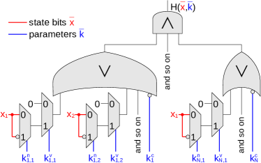
Figure 11: Circuit illustration of a generic CNF template.

Figure 11 shows a circuit that illustrates how the template $H(\overline{x},\overline{k})$ can be defined as a parameterized CNF formula over the state variables $\overline{x}$. That is, $F(\overline{x})$ is represented as a conjunction of clauses over the state variables. Template parameters $\overline{k}$ define the shape of the clauses. The trapezoids in Figure 11 are multiplexers that select one of the inputs on the left depending on the signal value fed in from below. A CNF encoding of this circuit such that it can be used in Equation (5) is straightforward [30].

The construction in Figure 11 works as follows. First, a maximum number $N$ of clauses is fixed. This number configures the expressiveness of the template. Next, three vectors $\overline{k^{c}}$, $\overline{k^{v}}$, $\overline{k^{n}}$ of template parameters are introduced. Together, they form $\overline{k}=\overline{k^{c}}\cup\overline{k^{v}}\cup\overline{k^{n}}$. The meaning of the parameters is as follows.

• If parameter $k^{c}_{i}$ with $1\leq i\leq N$ is $\mathsf{true}$, then clause $i$ is used in $F(\overline{x})$, otherwise not. This is achieved by making the clause $\mathsf{true}$ (and thus irrelevant in the conjunction of clauses) if $k^{c}_{i}$ is $\mathsf{false}$.

• If parameter $k^{v}_{i,j}$ with $1\leq i\leq N$ and $1\leq j\leq|\overline{x}|$ is $\mathsf{true}$, then the state variable $x_{j}\in\overline{x}$ appears in clause $i$ of $F(\overline{x})$, otherwise not. This is realized with a multiplexer that sets the corresponding literal in the clause to $\mathsf{false}$ (thus making it irrelevant in the disjunction) if $k^{v}_{i,j}$ is $\mathsf{false}$.

• If parameter $k^{n}_{i,j}$ is $\mathsf{true}$, then the state variable $x_{j}$ can appear in clause $i$ only negated, otherwise only unnegated. This is realized with a multiplexer that selects between $x_{j}$ and $\neg x_{j}$. If $k^{v}_{i,j}$ is $\mathsf{false}$, then $k^{n}_{i,j}$ is irrelevant.

This results in $|\overline{k}|=2\cdot N\cdot|\overline{x}|+N$ template parameters.

Example 14

For $\overline{x}=(x_{1},x_{2},x_{3})$ and $N=3$, the CNF $(x_{1}\vee\neg x_{2})\wedge(\neg x_{3})$ can be realized with

• $k^{c}_{1}=k^{c}_{2}=\mathsf{true}$ and $k^{c}_{3}=\mathsf{false}$ (only clause $1$ and $2$ are used),

• $k^{v}_{1,1}=k^{v}_{1,2}=\mathsf{true}$ and $k^{v}_{1,3}=\mathsf{false}$ (clause $1$ contains $x_{1}$ and $x_{2}$ but not $x_{3}$),

• $k^{v}_{2,3}=\mathsf{true}$ and $k^{v}_{2,1}=k^{v}_{2,2}=\mathsf{false}$ (clause $2$ contains $x_{3}$ but not $x_{1}$ and not $x_{2}$),

• $k^{n}_{1,1}=\mathsf{false}$ and $k^{n}_{1,2}=\mathsf{true}$ (clause $1$ contains $x_{1}$ unnegated and $x_{2}$ negated), and

• $k^{n}_{2,3}=\mathsf{true}$ (clause $2$ contains $x_{3}$ negated).

All other parameters are irrelevant.

Choosing $N$ is delicate. If $N$ is too low, we will not find a solution, even if one exists. If it is too high, we waste computational resources and may find an unnecessarily complex winning region. In our implementation, we solve this dilemma by starting with $N=1$ and increasing $N$ by one upon failure until we reach $N=4$. From there, we double $N$ upon failure. We stop if we get a negative answer for $N\geq 2^{|\overline{x}|}$ because any Boolean formula over $\overline{x}$ can be represented in a CNF with less than $2^{|\overline{x}|}$ clauses.

3.5.2 AND-Inverter Graph Templates

Another option is to define the template $H(\overline{x},\overline{k})$ as a network of AND-gates and inverters, fed by the state variables $\overline{x}$. The parameters $\overline{k}$ define the connections between the gates and the state variables, as well as the negation of signals.

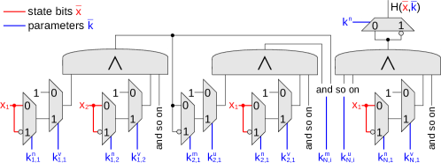
Figure 12: Circuit illustration of a generic AND-inverter graph template.

Figure 12 gives a concrete proposal for defining such a template. The template is again illustrated as a circuit, but can easily be encoded into CNF. A maximum number $N$ of AND-gates is chosen first. The first gate can have all state variables as input, either negated or unnegated. The second gate can also have the output of the first gate as input. The third gate can have the output of the first two gates as additional inputs, and so on. The output of the last AND-gate defines $H(\overline{x},\overline{k})$, again with a possible negation. The template parameters $\overline{k}$ define which inputs of a gates are actually used or ignored, and which inputs are used negated or unnegated. We distinguish five groups of parameters.

• If parameter $k^{v}_{i,j}$ with $1\leq i\leq N$ and $1\leq j\leq|\overline{x}|$ is $\mathsf{true}$, then $x_{j}\in\overline{x}$ appears as input of gate $i$, otherwise not.

• If parameter $k^{n}_{i,j}$ with $1\leq i\leq N$ and $1\leq j\leq|\overline{x}|$ is $\mathsf{true}$, then gate $i$ can only use the negated variable $x_{j}$ as input, otherwise only the unnegated variable.

• If $k^{u}_{i,j}$ with $1\leq i\leq N$ and $1\leq j<i$ is $\mathsf{true}$, then the output of gate $j$ is an input of gate $i$, otherwise not.

• If $k^{m}_{i,j}$ with $1\leq i\leq N$ and $1\leq j<i$ is $\mathsf{true}$, then gate $i$ can only use the negated output of gate $j$ as input, otherwise only the unnegated output.

• The single parameter $k^{n}$ defines if the output of the final gate defines $H(\overline{x},\overline{k})$ or $\neg H(\overline{x},\overline{k})$.

This gives $|\overline{k}|=N\cdot(2\cdot|\overline{x}|+N-1)+1$ template parameters.

Example 15

We continue Example 14, where $\overline{x}=(x_{1},x_{2},x_{3})$, $N=3$ and $F(\overline{x})=(x_{1}\vee\neg x_{2})\wedge(\neg x_{3})$, which can be rewritten to $\neg(\neg x_{1}\wedge x_{2})\wedge(\neg x_{3})$. This formula can be realized with

• $k^{v}_{2,1}=k^{v}_{2,2}=\mathsf{true}$ and $k^{v}_{2,3}=\mathsf{false}$ (gate $2$ uses $x_{1}$ and $x_{2}$ as input but not $x_{3}$),

• $k^{n}_{2,1}=\mathsf{true}$ and $k^{n}_{2,2}=\mathsf{false}$ (gate $2$ uses $x_{1}$ negated and $x_{2}$ unnegated),

• $k^{u}_{2,1}=\mathsf{false}$ (gate $2$ ignores the output of gate $1$),

• $k^{v}_{3,3}=\mathsf{true}$ and $k^{v}_{3,1}=k^{v}_{3,2}=\mathsf{false}$ (gate $3$ uses $x_{3}$ as input but not $x_{1}$ and not $x_{2}$),

• $k^{n}_{3,3}=\mathsf{true}$ (gate $3$ uses $x_{3}$ negated),

• $k^{u}_{3,2}=k^{m}_{3,2}=\mathsf{true}$ and $k^{u}_{3,1}=\mathsf{false}$ (gate $3$ uses the negated output of gate $2$ but ignores the output of gate $1$), and

• $k^{n}=\mathsf{false}$ (the output $H(\overline{x},\overline{k})$ is defined by the unnegated output of gate $3$).

All other parameters are irrelevant. In particular, the output of gate $1$ is completely ignored.

In our implementation, choosing $N$ works in the same way as for the CNF template: starting with $N=1$, $N$ is increased by $1$ in case of unsatisfiability of Equation (5) until $N=4$ is reached. From there, $N$ is doubled upon failure. There is a straightforward way to represent a CNF with $N$ clauses as a network of $N+1$ AND-gates. Hence, the criterion for detecting unrealizability with CNF templates can also be applied here: If Equation (5) is unsatisfiable for $N>2^{|\overline{x}|}$, the specification must be unrealizable.

3.5.3 Implementation with SAT Solvers

In this section, we present an extension of the Counterexample-Guided Inductive Synthesis (CEGIS) approach that allows us to compute satisfying assignments of Equation (5) with SAT solvers instead of a QBF solver.

Basic idea. Recall that CEGIS (see Section 2.6) is an approach to compute satisfying assignments in formulas of the form $\exists\overline{e}\operatorname{\mathbin{:}}\forall\overline{u}\operatorname{\mathbin{:}}F(\overline{e},\overline{u})$ by iterative refinements of a solution candidate. With

$$M(\overline{k},\overline{x},\overline{i},\overline{c},\overline{x}^{\prime})=\bigl{(}I(\overline{x})\rightarrow H(\overline{x},\overline{k})\bigr{)}\wedge\bigl{(}H(\overline{x},\overline{k})\rightarrow P(\overline{x})\bigr{)}\wedge\Bigl{(}H(\overline{x},\overline{k})\rightarrow\bigl{(}T(\overline{x},\overline{i},\overline{c},\overline{x}^{\prime})\wedge H(\overline{x}^{\prime},\overline{k})\bigr{)}\Bigr{)}$$

being an abbreviation for the matrix of the QBF in Equation (5), our task is now to compute a satisfying assignment for the parameters $\overline{k}$ in $\exists\overline{k}\operatorname{\mathbin{:}}\forall\overline{x},\overline{i}\operatorname{\mathbin{:}}\exists\overline{c},\overline{x}^{\prime}\operatorname{\mathbin{:}}M(\overline{k},\overline{x},\overline{i},\overline{c},\overline{x}^{\prime})$. Hence, there is an additional existential quantifier on the innermost level. This existential quantifier does not affect the computation of solution candidates significantly: Candidates are satisfying assignments for the variables $\overline{k}$ in $\bigwedge_{(\mathbf{x},\mathbf{i})\in D}\exists\overline{c},\overline{x}^{\prime}\operatorname{\mathbin{:}}M(\overline{k},\mathbf{x},\mathbf{i},\overline{c},\overline{x}^{\prime}),$ where the existential quantification of $\overline{c}$ and $\overline{x}^{\prime}$ can be handled by renaming these variables in every copy of $M$ and then calling a SAT solver. The computation of counterexamples, i.e., values for the variables $\overline{x}$ and $\overline{i}$, becomes more intricate, though. Instead of a satisfying assignment for $\neg F(\mathbf{e},\overline{u})$, we now need to compute an assignment $\mathbf{x},\mathbf{i}$ for the variables $\overline{x},\overline{i}$ in $\neg\exists\overline{c},\overline{x}^{\prime}\operatorname{\mathbin{:}}M(\mathbf{k},\overline{x},\overline{i},\overline{c},\overline{x}^{\prime}),$ where $\mathbf{k}$ represents fixed values for the variables $\overline{k}$. The negation turns the existential quantification into a universal one. The resulting quantifier alternation prevents us from computing counterexamples with a single call to a SAT solver. A QBF solver could be used, but the idea of this section is to substitute QBF solving with plain SAT solving. Hence, we will use an iterative approach that is similar to SatWin1 in Algorithm 9 to compute counterexamples.

Algorithm 10 TemplWinSat: An algorithm to compute template instantiations using SAT solvers.

1:procedure TemplWinSat$\left(H(\overline{x},\overline{k}),(\overline{x},\overline{i},\overline{c},I,T,P)\right)$, returns: A winning area $F(\overline{x})$ or “fail”

2:   $G(\overline{k},\overline{t}):=\mathsf{true}$

3:   while $\mathsf{true}$ do

4:      if $\textsf{sat}=\mathsf{false}$ in $(\textsf{sat},\mathbf{k}):=\textsc{PropSatModel}\bigl{(}G(\overline{k},\overline{t})\bigr{)}$ then

5:         return “fail”       

6:      if $\textsf{correct}=\mathsf{true}$ in $(\textsf{correct},\mathbf{x},\mathbf{i}):=\textsc{Check}\bigl{(}H(\overline{x},\mathbf{k}),(\overline{x},\overline{i},\overline{c},I,T,P)\bigr{)}$  then

7:         return $H(\overline{x},\mathbf{k})$       

8:      $\overline{t}_{c}:=\textsf{CreateFreshCopy}(\overline{c})$,  $\overline{t}_{x}:=\textsf{CreateFreshCopy}(\overline{x}^{\prime})$

9:      $G(\overline{k},\overline{t}):=G(\overline{k},\overline{t})\wedge\bigl{(}I(\mathbf{x})\rightarrow H(\mathbf{x},\overline{k})\bigr{)}\wedge\bigl{(}H(\mathbf{x},\overline{k})\rightarrow P(\mathbf{x})\bigr{)}\wedge\bigl{(}H(\mathbf{x},\overline{k})\rightarrow\bigl{(}T(\mathbf{x},\mathbf{i},\overline{t}_{c},\overline{t}_{x})\wedge H(\overline{t}_{x},\overline{k})\bigr{)}\bigr{)}$    

10:procedure Check$\left(F(\overline{x}),(\overline{x},\overline{i},\overline{c},I,T,P)\right)$, returns: $(\textsf{correct},\mathbf{x},\mathbf{i})$

11:   if $\mathsf{sat}=\mathsf{true}$ in $(\mathsf{sat},\mathbf{x}):=\textsc{PropSatModel}\bigl{(}(I(\overline{x})\wedge\neg F(\overline{x}))\vee(F(\overline{x})\wedge\neg P(\overline{x}))\bigr{)}$  then

12:      return $(\mathsf{true},\mathbf{x},\bigwedge_{i\in\overline{i}}\neg i)$    

13:   $U(\overline{x},\overline{i}):=\mathsf{true}$

14:   while $\mathsf{true}$ do

15:      if $\mathsf{sat}=\mathsf{false}$ in $(\mathsf{sat},\mathbf{x},\mathbf{i}):=\textsc{PropSatModel}\bigl{(}F(\overline{x})\wedge U(\overline{x},\overline{i})\wedge T(\overline{x},\overline{i},\overline{c},\overline{x}^{\prime})\wedge\neg F(\overline{x}^{\prime})\bigr{)}$  then

16:         return $(\mathsf{true},\mathsf{true},\mathsf{true})$       

17:      if $\mathsf{sat}=\mathsf{false}$ in $(\mathsf{sat},\mathbf{c}):=\textsc{PropSatModel}\bigl{(}F(\overline{x})\wedge\mathbf{x}\wedge\mathbf{i}\wedge T(\overline{x},\overline{i},\overline{c},\overline{x}^{\prime})\wedge F(\overline{x}^{\prime})\bigr{)}$  then

18:         return $(\mathsf{false},\mathbf{x},\mathbf{i})$

19:      else

20:         $U(\overline{x},\overline{i}):=U(\overline{x},\overline{i})\wedge\neg\textsc{PropMinUnsatCore}\bigl{(}\mathbf{x}\wedge\mathbf{i},\mathbf{c}\wedge F(\overline{x})\wedge U(\overline{x},\overline{i})\wedge T(\overline{x},\overline{i},\overline{c},\overline{x}^{\prime})\wedge\neg F(\overline{x}^{\prime})\bigr{)}$          

Algorithm. The procedure TemplWinSat in Algorithm 10 takes as input a template $H(\overline{x},\overline{k})$ for a winning area as well as a safety specification $\mathcal{S}$. As output, it returns either a concrete winning area $F(\overline{x})$ as an instantiation of the template $H(\overline{x},\overline{k})$, or “fail” of no instantiation of $H(\overline{x},\overline{k})$ can be a winning area. The structure of the algorithm is the same as for CegisSmt in Algorithm 5: The formula $G(\overline{k},\overline{t})$ accumulates constraints that the template parameters $\overline{k}$ have to satisfy, where $\overline{t}$ is a vector of auxiliary variables. Line 4 computes candidate template parameter values $\mathbf{k}$ in form of a satisfying assignment for $G$. If the formula is unsatisfiable, then no template instantiation can be a winning area and the procedure returns “fail”. If the formula is satisfiable, a candidate winning area $F(\overline{x})=H(\overline{x},\mathbf{k})$ is computed using the parameter values $\mathbf{k}$. Next, the candidate is checked in Line 6. This step is different to CegisSmt in Algorithm 5 and explained in the next paragraph. If the candidate is correct, it is returned. Otherwise, the procedure Check returns a counterexample in form of a satisfying assignment $\mathbf{x},\mathbf{i}$ for the variables $\overline{x},\overline{i}$. The meaning of this counterexample is that $\exists\overline{c},\overline{x}^{\prime}\operatorname{\mathbin{:}}\bigl{(}I(\mathbf{x})\rightarrow H(\mathbf{x},\mathbf{k})\bigr{)}\wedge\bigl{(}H(\mathbf{x},\mathbf{k})\rightarrow P(\mathbf{x})\bigr{)}\wedge\bigl{(}H(\mathbf{x},\mathbf{k})\rightarrow\bigl{(}T(\mathbf{x},\mathbf{i},\overline{c},\overline{x}^{\prime})\wedge H(\mathbf{x}^{\prime},\mathbf{k})\bigr{)}\bigr{)}$ does not hold, thus witnessing that $\mathbf{k}$ cannot be a solution to Equation (5) yet. To make sure the candidate of the next iteration works also for the counterexample $\mathbf{x},\mathbf{i}$, the constraints on $\overline{k}$ are refined accordingly in Line 9. The variables $\overline{c}$ and $\overline{x}^{\prime}$ are renamed to fresh auxiliary variables in order to account for their existential quantification.

Counterexample computation. The procedure Check in Algorithm 10 is a helper routine for TemplWinSat that checks if a given candidate $F(\overline{x})$ is a winning area. It returns $\textsf{correct}=\mathsf{true}$ if this is the case. Otherwise, it sets $\textsf{correct}=\mathsf{false}$ and returns a counterexample $\mathbf{x},\mathbf{i}$ witnessing the incorrectness. Line 11 checks if the first two properties in the definition of a winning area $F$, namely $I\rightarrow F$ and $F\rightarrow P$, are satisfied (see Definition 5). If this is not the case, a satisfying assignment $\mathbf{x}$ is returned as a counterexample witnessing this defect. The input vector $\mathbf{i}$ returned as part of the counterexample is irrelevant in this case. Otherwise, Check turns to verifying the third property of a winning area, namely $F\rightarrow\mathsf{Force}^{s}_{1}(F)$. Here, we search for a counterexample $\mathbf{x},\mathbf{i}$ such that no value $\mathbf{c}$ can prevent the system from leaving $F(\overline{x})$ if the environment picks input $\mathbf{i}$ from state $\mathbf{x}\models F(\overline{x})$. The same kind of counterexample computation was performed already by SatWin1 in Algorithm 9, so we simply reuse this algorithm here. The difference is that $F(\overline{x})$ is not refined by Check. Thus, there is no need for lazy updates of $\neg F(\overline{x}^{\prime})$, which renders quite some lines of Algorithm 9 obsolete.

An optimization. The check in Line 11 of Algorithm 10 can actually be omitted if we ensure that $\forall\overline{x},\overline{k}\operatorname{\mathbin{:}}I(\overline{x})\rightarrow H(\overline{x},\overline{k})$ and $\forall\overline{x},\overline{k}\operatorname{\mathbin{:}}H(\overline{x},\overline{k})\rightarrow P(\overline{x})$ holds by the construction of the template $H(\overline{x},\overline{k})$. This can easily be achieved by taking any template $H^{\prime}(\overline{x},\overline{k})$ and defining a new template $H(\overline{x},\overline{k})=\bigl{(}H^{\prime}(\overline{x},\overline{k})\wedge P(\overline{x})\bigr{)}\vee I(\overline{x})$, given that $I(\overline{x})\wedge\neg P(\overline{x})$ is unsatisfiable (otherwise the specification is trivially unrealizable). We use this optimization in our implementation.

Incremental solving. Algorithm 10 is well suited for incremental SAT solving. We propose to use three solver instances. The first one stores $G$ and is used for Line 4. Constraints are only added to $G$ in Line 9, so no re-initialization is needed. The second solver instances stores $F(\overline{x})\wedge U(\overline{x},\overline{i})\wedge T(\overline{x},\overline{i},\overline{c},\overline{x}^{\prime})\wedge\neg F(\overline{x}^{\prime})$ and is used in Line 15 and 20. It is (re-)initialized when Check is called. After that, clauses are only added to $U$ in Line 20. Finally, the third solver instance stores $F(\overline{x})\wedge T(\overline{x},\overline{i},\overline{c},\overline{x}^{\prime})\wedge F(\overline{x}^{\prime})$ and is used in Line 17. This instance is also (re-)initialized whenever Check is called. This CNF does not change at all during the execution of Check. The conjunctions with $\mathbf{x}$, $\mathbf{i}$ and $\mathbf{c}$ are realized with assumption literals that are temporarily asserted.

3.5.4 Discussion

The template-based approach has a potential for finding simple winning areas quickly. There may exist many winning areas that satisfy the constraints given by Definition 5. The algorithms SafeWin, QbfWin and SatWin1 discussed earlier will always compute the largest possible winning area (modulo unreachable states if used with optimization RG or RC). The template-based approach is more flexible in this respect. As an extreme example, suppose that there is only one initial state, it is safe, and the system can enforce that the play stays in this state. Suppose further that the winning region is complicated. The template-based approach may find $F=I$ quickly, while the other approaches may require many iterations to compute the winning region.

On the other hand, the template-based approach can be expected to scale poorly if no simple winning area exists or if the synthesis problem is unrealizable. Starting with a small expressiveness parameter $N$, Equation (5) will be unsatisfiable, so $N$ is increased. With increasing $N$, the search space for the solver increases, which results in longer execution times. For unrealizable specifications, we can only terminate once $N>2^{|\overline{x}|}$ (when using our CNF or AND-inverter graph templates). Except for specifications with a very low numbers of state variables, a timeout is likely to be hit before this point can be reached.

3.6 Reduction to Effectively Propositional Logic (EPR)

The template-based approach presented in the previous section may work well if a simple representation of a winning area exists. However, one drawback is the need to select a template, which is a delicate matter. It would be more desirable to directly compute a winning area as a Skolem function of a quantified formula. Unfortunately, the definition of a winning area (Definition 5) not only involves the winning area $F(\overline{x})$ but also its next-state copy $F(\overline{x}^{\prime})$. Hence, we have to compute two Skolem functions, and the two functions have to be functionally consistent. This problem cannot be formulated as a QBF formula with a linear quantifier prefix, but requires more expressive logics.

3.6.1 Using Henkin Quantifiers

One solution is to use so-called Henkin quantifiers [69], which are quantifiers that are only partially ordered. This partial order can be used to restrict variable dependencies. In particular, a winning area $F(\overline{x})$ can be computed as a Skolem function for the variable $w$ in

$$\begin{array}[]{l}\forall\overline{x}\operatorname{\mathbin{:}}\exists w\operatorname{\mathbin{:}}\forall\overline{i}\operatorname{\mathbin{:}}\exists\overline{c}\operatorname{\mathbin{:}}\\ \forall\overline{x}^{\prime}\operatorname{\mathbin{:}}\exists w^{\prime}\operatorname{\mathbin{:}}\end{array}\bigl{(}I(\overline{x})\rightarrow w\bigr{)}\wedge\bigl{(}w\rightarrow P(\overline{x})\bigr{)}\wedge\bigl{(}w\wedge T(\overline{x},\overline{i},\overline{c},\overline{x}^{\prime})\rightarrow w^{\prime}\bigr{)}\wedge\bigl{(}(\overline{x}=\overline{x}^{\prime})\rightarrow(w=w^{\prime})\bigr{)}.$$

This formulation ensures that the Skolem function $F(\overline{x})$ for $w$ can only depend on $\overline{x}$, and the Skolem function $G(\overline{x}^{\prime})$ for $w^{\prime}$ can only depend on $\overline{x}^{\prime}$. The last constraint enforces functional consistency between $F$ and $G$, i.e., $F$ and $G$ are actually the same function but applied to different parameters. The logic of applying Henkin quantifiers to propositional formulas is called Dependency Quantified Boolean Formulas (DQBF) and was first described by Peterson and Reif [70]. Deciding whether a DQBF formula is satisfiable is NEXPTIME complete [70]. In addition to this high complexity, only a few approaches and tools to solve DQBF formulas have recently been proposed [71, 72]. For this reason, we did not implement a DQBF-based solution but we rather use EPR, where mature solvers are available.

3.6.2 Using Effectively Propositional Logic (EPR)

Recall from Section 2.1.4 that EPR is the set of first-order logic formulas of the form $\exists\overline{x}\operatorname{\mathbin{:}}\forall\overline{y}\operatorname{\mathbin{:}}F(\overline{x},\overline{y})$, where $F$ is a quantifier-free formula in CNF that must not contain function symbols but can contain predicate symbols. These predicate symbols are implicitly quantified existentially. We seek a winning area $F(\overline{x})$ satisfying the three properties of Definition 5, which can be combined to

$$\exists F\operatorname{\mathbin{:}}\forall\overline{x},\overline{i}\operatorname{\mathbin{:}}\exists\overline{c},\overline{x}^{\prime}\operatorname{\mathbin{:}}\bigl{(}I(\overline{x})\rightarrow F(\overline{x})\bigr{)}\wedge\bigl{(}F(\overline{x})\rightarrow P(\overline{x})\bigr{)}\wedge\Bigl{(}F(\overline{x})\rightarrow\bigl{(}T(\overline{x},\overline{i},\overline{c},\overline{x}^{\prime})\wedge F(\overline{x}^{\prime})\bigr{)}\Bigr{)}.$$

In order to transform this constraint into EPR, we need to perform several steps, which are similar to those by Seidl et al. [73] when transforming QBF formulas into EPR.

Step 1. We replace all the Boolean variables $\overline{x},\overline{i},\overline{c},\overline{x}^{\prime}$ by corresponding first-order domain variables. Since the original variables can only take two different values, we introduce a unary predicate $V$ to represent the truth value of a domain variable. We also introduce two domain constants $\top$ and $\bot$ to encode $\mathsf{true}$ and $\mathsf{false}$, and add the axioms $V(\top)$ and $\neg V(\bot)$ to the final EPR formula.

Step 2. We introduce predicate symbols $I(\overline{x})$, $P(\overline{x})$, $T(\overline{x},\overline{i},\overline{c},\overline{x}^{\prime})$ and $F(\overline{x})$ to represent the different parts of the formula. The predicates $I$, $P$ and $T$ are equipped with additional constraints that fully define their truth value based on the truth values of the variables on which they depend. The predicate $F$ is left unconstrained because it represents the winning area we wish to compute.

Step 3. We eliminate the existential quantification over $\overline{c}$ and $\overline{x}^{\prime}$. Since $T$ is deterministic and complete (Definition 4), the one-point rule (2) can be used to eliminate the existential quantification over $\overline{x}^{\prime}$:

$$\exists F\operatorname{\mathbin{:}}\forall\overline{x},\overline{i}\operatorname{\mathbin{:}}\exists\overline{c}\operatorname{\mathbin{:}}\forall\overline{x}^{\prime}\operatorname{\mathbin{:}}\bigl{(}I(\overline{x})\rightarrow F(\overline{x})\bigr{)}\wedge\bigl{(}F(\overline{x})\rightarrow P(\overline{x})\bigr{)}\wedge\Bigl{(}\bigl{(}F(\overline{x})\wedge T(\overline{x},\overline{i},\overline{c},\overline{x}^{\prime})\bigr{)}\rightarrow F(\overline{x}^{\prime})\Bigr{)}.$$

The existential quantification over $\overline{c}$ is eliminated by Skolemization: for every $c_{j}\in\overline{c}$, we introduce a new predicate $C_{j}(\overline{x},\overline{i})$. All occurrences of $V(c_{j})$ in the definition of $T$ are then replaced by $C_{j}(\overline{x},\overline{i})$. This gives a formula of the form

$$\exists F,C_{1},\ldots,C_{|\overline{c}|}\operatorname{\mathbin{:}}\forall\overline{x},\overline{i},\overline{x}^{\prime}\operatorname{\mathbin{:}}\bigl{(}I(\overline{x})\rightarrow F(\overline{x})\bigr{)}\wedge\bigl{(}F(\overline{x})\rightarrow P(\overline{x})\bigr{)}\wedge\Bigl{(}\bigl{(}F(\overline{x})\wedge T(\overline{x},\overline{i},\overline{x}^{\prime})\bigr{)}\rightarrow F(\overline{x}^{\prime})\Bigr{)}.$$

Step 4. The body of the resulting formula needs to be encoded into CNF. Since we have a conjunction of implications on the top-level, this is mainly a matter of encoding the constraints defining $I$, $P$ and $T$ into CNF. Note that the standard Tseitin [30] or Plaisted-Greenbaum [31] transformations introduce new auxiliary variables that are quantified existentially on the innermost level. Since this is not allowed in EPR, these auxiliary variables need to be eliminated again. Similar to the elimination of the variables $\overline{c}$ in Step 3, we do this by introducing new predicates. To increase efficiency, we do not pass all variables of $\overline{x},\overline{i},\overline{x}^{\prime}$ as arguments to the new predicates, but rather analyze the variable dependencies structurally and pass only the relevant ones.

Solving the resulting EPR formula. We call iProver on the resulting EPR formula. iProver is an instantiation-based first-order theorem prover that can produce implementations for the predicates that occur in the formula. This means that the solver directly returns a winning area $F(\overline{x})$. Since we represent the truth values of the variables $c_{j}\in\overline{c}$ with predicates $C_{j}(\overline{x},\overline{i})$, we can also extract an implementation from the solver result. That is, there is no need to apply the circuit construction methods that will be presented in Chapter 4 when using the EPR synthesis approach.

Discussion. Similar to the template-based approach from Section 3.5, this approach does not compute the winning region but some winning area. It can thus benefit from situations where the winning region is complicated but a simple winning area exists. In contrast to the template-based approach, there is no need to guess a template and to increase the expressiveness of the template if no solution is found. The price that is payed for this benefit is the higher worst-case complexity for checking the satisfiability of the constructed formulas because a more expressive logic is used.

3.7 Parallelization

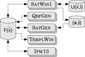
Figure 13: Parallelized strategy computation.

The various methods for strategy computation presented so far have different strengths and weaknesses and, consequently, perform well on different classes of benchmarks. To a smaller extent, different characteristics can also be observed within one method when run with different optimizations or solvers. In this section, we thus combine different methods and configurations in the hope to inherit all their strengths while compensating their weaknesses. We do this in a parallelized way, where individual methods are running in separate threads but share discovered information that may be helpful for others.

Figure 13 gives a proposal for combining a promising subset of the methods (or fragments thereof). Arrows denote information that is exchanged between threads.

SatWin1 threads. The SatWin1 threads execute the SatWin1 procedure from Algorithm 9 and can be seen as the main workhorse. Individual SatWin1 threads can be run with or without optimization RG, with or without quantifier expansion, and with different SAT solvers. All newly discovered clauses of the winning region $F(\overline{x})$ are put into a central database and communicated to the other threads. Newly discovered $U$-clauses are also shared between SatWin1 threads. In order for this to work, the SatWin1 threads need be synchronized regarding their restarts of solverC, i.e., they need to work with the same version of $\neg G(\overline{x}^{\prime})$ at any time. If several SatWin1 threads are running in a mode where they perform universal expansion, the expansion is only done by one thread (while the others sleep) in order not to waste resources (like stressing the memory bus unnecessarily).

QbfGen threads. The QbfGen threads take existing clauses from $F$ and attempt to generalize them further by eliminating more literals. This is done as in Line 5 to Line 9 of the QbfWin procedure in Algorithm 6 using a QBF solver. If a clause could be shortened, the reduced clause is communicated to all other threads. Individual QbfGen threads can be run with or without optimization RG, with or without QBF preprocessing, and with or without incremental QBF solving (the combination of incremental solving plus preprocessing is not available).

SatGen threads. These threads take counterexamples $(\mathbf{x},\mathbf{i})$, as computed by the SatWin1 threads, and compute all generalizations using a SAT solver (as illustrated in Figure 7). The resulting $F$-clauses are shared.

TemplWin threads. These threads implement the template-based method from Section 3.5, using CNF templates of increasing size. The clauses from $F$ are considered as fixed over-approximation of the winning area to compute — the threads only compute additional clauses such that a winning area is obtained. A timeout of $20$ seconds makes the thread try again (with a potentially refined set $F$ of fixed clauses) if a solution cannot be found quickly. The short timeout is justified by the observation that the template-based approach either finds a solution quickly or not at all. The QBF-based implementation and the SAT-based implementation of the template-based approach are alternated from timeout to timeout. The TemplWin threads are information sinks: the only information communicated back to other threads is a request to terminate if a solution has been found.

Ifm’13 threads. These threads execute a reimplementation of the SAT-based synthesis method proposed by Morgenstern et al. [74]. This method maintains an over-approximation $G(\overline{x})$ of the winning region $W(\overline{x})$ as well as over-approximations of sets of states from which the environment can win the game in different numbers of steps. We couple $G(\overline{x})$ with $F(\overline{x})$: If new clauses are added to $G(\overline{x})$, then they are also added to $F(\overline{x})$ and communicated to the other threads. If other threads discover new $F$-clauses, they are also added to $G$ in the Ifm’13 threads.

Configuration. When only one thread is available, we make it execute SatWin1 with optimization RG, quantifier expansion and MiniSat as underlying SAT solver. If two threads are available, the second one executes TemplWin (with DepQBF, Bloqqer and MiniSat). If three threads are available, the third thread runs Ifm’13 using MiniSat. With four threads, we also use a second instance of SatWin1, but with quantifier expansion disabled. With five threads, we also include a SatGen thread, and with six threads we also include a QbfGen thread.

Variations. The current realization always shares all discovered clauses that refine the winning region with all other threads. Another option is to share only small clauses (where the number of literals is below some threshold) in order to reduce the communication overhead. In general, smaller clauses refine the winning region more substantially than larger ones, so this approach would focus on communicating only significant findings. Another promising extension is to include also threads that run BDD-based algorithms, e.g., a BDD-based realization of Algorithm 1. The BDD-based threads can directly use clauses discovered by other threads to refine the BDD that represents the winning region. Communication in the other direction is possible as well: many BDD libraries provide functions to convert a BDD into CNF. While it may be expensive to share all clauses of such a CNF translation, it may still be beneficial to factor out a set of small clauses and communicate them.

Discussion. The main purpose of our parallelization is to combine different methods that complement each other. Exploiting hardware parallelism in only a secondary aspect because, due to the high worst-case complexities, even a speedup factor of, say, $10$ may have little impact on the ability of solving larger benchmark instances. Furthermore, we do not claim that our choice of distributing workload over the threads is in any way optimal. We rather selected the methods to run in individual threads quite greedily, based on the performance results when running methods in isolation (see Chapter 5) and based on experiments with subsets of the benchmarks. However, there is such a plethora of possibilities for combining different methods, fragments thereof, optimizations, heuristics and solver configurations that finding particularly good configurations is quite an intricate task. Hence, we rather see the main contribution of our parallelization in providing a “playground” for combining different approaches and configurations. It demonstrates that a parallelized way of combining different SAT-based synthesis approaches is easily possible. This stands in contrast to BDD-based synthesis algorithms, where a parallelization is often much more difficult to achieve. Our parallelization goes far beyond a pure portfolio approach because fine-grained information about refinements of the winning region, discovered counterexamples and unsuccessful attempts to compute counterexamples is exchanged between the threads as soon as discovered. This information can speed up the progress in other threads and thus stimulate “cross-fertilization” effects.

4 From Strategies to Circuits

In Chapter 3, we presented a number of SAT-based methods to compute a strategy for defining the control signals $\overline{c}$ such that a given safety specification is enforced. Recall that such a strategy is a formula $S(\overline{x},\overline{i},\overline{c},\overline{x}^{\prime})$ such that $\forall\overline{x},\overline{i}\operatorname{\mathbin{:}}\exists\overline{c},\overline{x}^{\prime}\operatorname{\mathbin{:}}S(\overline{x},\overline{i},\overline{c},\overline{x}^{\prime}).$ That is, for every state $\mathbf{x}$ and input $\mathbf{i}$, the strategy will contain at least one vector of control values $\mathbf{c}$ that is allowed in this situation. In many situations, many control values can be allowed, though. The task is now to compute a system implementation in form of a function $f:2^{\overline{x}}\times 2^{\overline{i}}\rightarrow 2^{\overline{c}}$ to uniquely define the control signals $\overline{c}$ based on the current state variables $\overline{x}$ and the uncontrollable inputs $\overline{i}$. The system implementation $f$ is supposed to implement the strategy in the sense that $\forall\overline{x},\overline{i}\operatorname{\mathbin{:}}\exists\overline{x}^{\prime}\operatorname{\mathbin{:}}S\bigl{(}\overline{x},\overline{i},f(\overline{x},\overline{i}),\overline{x}^{\prime}\bigr{)}$ holds. That is, for all concrete assignments $\mathbf{x},\mathbf{i}$, the control variable assignment $\mathbf{c}=f(\mathbf{x},\mathbf{i})$ computed by $f$ must be allowed by the strategy $S$. Finally, this function $f$ needs to be implemented as a circuit. Obviously, we prefer fast algorithms that produce small circuits. In order to achieve this, the freedom in the strategy relation $S$ needs to be exploited cleverly.

A cofactor-based algorithm to solve the problem has already been presented in Section 2.4.3. It can be seen as the “standard method” for computing an implementation from a strategy, and can easily be implemented using BDDs. In the following subsections, we will present alternative approaches that use SAT- or QBF solvers instead. The presented approaches are not specific to safety specifications. However, in many cases, the specific structure of strategies $S(\overline{x},\overline{i},\overline{c},\overline{x}^{\prime})=T(\overline{x},\overline{i},\overline{c},\overline{x}^{\prime})\wedge\bigl{(}W(\overline{x})\rightarrow W(\overline{x}^{\prime})\bigr{)}$ for safety specifications can be exploited. We will thus always present the general approach first, and then discuss an efficient implementation for safety synthesis problems. As a preprocessing step to all our methods, we simplify $W$ by calling CompressCnf (see Algorithm 7) with literal dropping enabled in order to remove redundant literals and clauses from $W$. As a postprocessing step to all our methods, we invoke the tool ABC [67] in order to reduce the size of the produced circuits.

4.1 QBF Certification

A system implementation can be computed as Skolem function for the signals $\overline{c}$ in $\forall\overline{x},\overline{i}\operatorname{\mathbin{:}}\exists\overline{c},\overline{x}^{\prime}\operatorname{\mathbin{:}}S(\overline{x},\overline{i},\overline{o},\overline{x}^{\prime})$. The QBFCert [25] framework by Niemetz et al. computes such Skolem functions for satisfiable QBFs from proof traces produced by the DepQBF [48] solver. The resulting Skolem functions are produced as circuits in AIGER format. Hence, in our setting, a single call to QBFCert suffices to compute a system implementation in form of a circuit.

4.1.1 Efficient Implementation for Safety Synthesis Problems

While the basic approach is simple, we can still apply some optimizations to increase the efficiency for the case of safety synthesis problems.

QBF formulation. Instead of computing a Skolem function for the variables $\overline{c}$ in the formula

$$\forall\overline{x},\overline{i}\operatorname{\mathbin{:}}\exists\overline{c},\overline{x}^{\prime}\operatorname{\mathbin{:}}T(\overline{x},\overline{i},\overline{c},\overline{x}^{\prime})\wedge\bigl{(}W(\overline{x})\rightarrow W(\overline{x}^{\prime})\bigr{)}$$ (6)

we rather compute a Herbrand function in its negation $\exists\overline{x},\overline{i}\operatorname{\mathbin{:}}\forall\overline{c},\overline{x}^{\prime}\operatorname{\mathbin{:}}\neg T(\overline{x},\overline{i},\overline{c},\overline{x}^{\prime})\vee\bigl{(}W(\overline{x})\wedge\neg W(\overline{x}^{\prime})\bigr{)}.$ Because $T$ is both deterministic and complete (Definition 4), the one-point rule (2) can be applied to turn the universal quantification over $\overline{x}^{\prime}$ into an existential quantification:

$$\exists\overline{x},\overline{i}\operatorname{\mathbin{:}}\forall\overline{c}\operatorname{\mathbin{:}}\exists\overline{x}^{\prime}\operatorname{\mathbin{:}}T(\overline{x},\overline{i},\overline{c},\overline{x}^{\prime})\wedge W(\overline{x})\wedge\neg W(\overline{x}^{\prime}).$$ (7)

Just like most QBF solvers, QBFCert requires a PCNF as input. Since most of our methods to compute a winning region (or winning area) produce $W$ in CNF, we only need to transform $T$ and $\neg W(\overline{x}^{\prime})$ into CNF. In contrast, using Equation (6) would require an additional CNF encoding of the implication $W(\overline{x})\rightarrow W(\overline{x}^{\prime})$. Another advantage of using Equation (7) lies in the size of the proofs: since the QBF is now unsatisfiable, the QBFCert framework processes a clause resolution proof instead of a cube resolution proof. These clause resolution proofs are often smaller.

Algorithm 11 NegLearn: Computing a CNF representation for the negation of a formula $F(\overline{x})$.

1:procedure NegLearn$\left(F(\overline{x})\right)$, returns: $\neg F(\overline{x})$ in CNF

2:   $N(\overline{x}):=\mathsf{true}$

3:   while $\mathsf{sat}=\mathsf{true}$ in $(\mathsf{sat},\mathbf{x}):=\textsc{PropSatModel}\bigl{(}F(\overline{x})\wedge N(\overline{x})\bigr{)}$ do

4:      $N(\overline{x}):=N(\overline{x})\wedge\neg\textsc{PropMinUnsatCore}\bigl{(}\mathbf{x},\neg F(\overline{x})\bigr{)}$    

5:   return $N(\overline{x})$

Negation of $W(\overline{x}^{\prime})$. For complex benchmarks, the auxiliary files produced by QBFCert can still grow very large (hundreds of GB). One reason is that a straightforward CNF encoding of $\neg W(\overline{x}^{\prime})$ requires many auxiliary variables and clauses. We can reduce the size of the auxiliary files (by up to a factor of 30 in our experiments) by computing a CNF representation of $\neg W(\overline{x}^{\prime})$ without introducing auxiliary variables. The procedure NegLearn in Algorithm 11 computes such a negation with query learning. It follows the principle of CnfLearn, shown in Algorithm 4, and uses a SAT solver to implement the queries: As long as $N$ is not yet equivalent to $\neg F$, i.e., $F\wedge N$ is still satisfiable, NegLearn refines $N$ with a clause that excludes the cube $\mathbf{x}$ witnessing this insufficiency. By taking the unsatisfiable core, the clause eliminates also other counterexamples. Since clauses are only added to $N$, NegLearn is well suited for incremental SAT solving.

4.1.2 Discussion

Dependencies between control signals. In contrast to CofSynt from Algorithm 2, the QBF certification approach computes a circuit for all control signals simultaneously. This can be both an advantage and a disadvantage. The advantage is that dependencies between control signals can potentially be handled more effectively. CofSynt can only take local decisions and fixes an implementation for one control signal without considering the consequences on other control signals (as long as some solution for the other signals still exist). The QBF certification approach is free to make global decisions when fixing the individual circuits. On the other hand, considering all control signals simultaneously instead of decomposing the problem into smaller subproblems can also be a scalability disadvantage.

Dependencies on reasoning engine. The performance of QBFCert as well as the quality of the resulting circuit depend on the ability of DepQBF to find a compact unsatisfiability proof quickly. In this sense, the technique strongly depends on the underlying symbolic reasoning engine. This is similar to CofSynt when implemented using BDDs, where the ability to find a good variable ordering can influence the circuit size and the execution time heavily.

4.2 QBF-Based Query Learning

In this section, we introduce an approach that is also based on QBF solving, but constructs circuits for one control signal after the other. In this respect, it is more similar to CofSynt presented in Algorithm 2. However, in contrast to CofSynt, we rely on query learning to exploit implementation freedom in the strategy in order to obtain small circuits.

The query learning algorithms introduced in Section 2.5 compute a certain representation of a given target formula $G(\overline{x})$ precisely. That is, the resulting formula $F(\overline{x})$ will be equivalent to the target $G(\overline{x})$. This is achieved by starting with some initial approximation for $F$, and refining this approximation based on counterexamples witnessing that $F\neq G$. These counterexamples are also generalized to speed up the progress. The same formula $G$ is used both for computing counterexamples and for generalizing them. However, by using two different formulas $G_{1}$ and $G_{2}$ in these two phases, we can also compute a function $F$ such that $G_{1}\rightarrow F\rightarrow G_{2}$. This idea can be used to exploit freedom in defining $F$, where the freedom is defined by (the difference between) $G_{1}$ and $G_{2}$. Note that $F$ is actually an interpolant for $G_{1}\wedge\neg G_{2}$ (see Section 2.1.1). Thus, this way of query learning with freedom can be seen as a special way to compute interpolants. However, depending on the underlying reasoning engine used in query learning, the formulas $G_{1}$ and $G_{2}$ do not have to be quantifier-free. Furthermore, by choosing an appropriate learning algorithm, we can control the shape of $F$. For instance, a CNF learning algorithm will produce $F$ in form of a CNF formula.

In the following, we will present a circuit synthesis algorithm based on CNF learning using a QBF solver. CNF learning is particularly suitable in this setting because QBF solvers require formulas in PCNF, so building up the solution in CNF reduces the overhead (especially in terms of formula size) imposed by CNF transformations. Solutions with other learning algorithms have been proposed by Ehlers et al. [61]. After introducing the basic algorithm, we will also discuss an efficient realization for safety synthesis problems.

4.2.1 QBF-Based CNF Learning

Algorithm 12 QbfSynt: Synthesizing circuits with QBF-based CNF learning.

1:procedure QbfSynt($S(\overline{x},\overline{i},\overline{c},\overline{x}^{\prime})$)

2:   for $c_{j}\in\overline{c}$ do

3:      $M_{1}(\overline{x},\overline{i}):=\forall\overline{c},\overline{x}^{\prime}\operatorname{\mathbin{:}}\neg S\bigl{(}\overline{x},\overline{i},(c_{0},\ldots,c_{j-1},\mathsf{false},c_{j+1},\ldots,c_{n}),\overline{x}^{\prime}\bigr{)}$

4:      $M_{0}(\overline{x},\overline{i}):=\forall\overline{c},\overline{x}^{\prime}\operatorname{\mathbin{:}}\neg S\bigl{(}\overline{x},\overline{i},(c_{0},\ldots,c_{j-1},\mathsf{true},c_{j+1},\ldots,c_{n}),\overline{x}^{\prime}\bigr{)}$

5:      $F_{j}(\overline{x},\overline{i}):=\mathsf{true}$

6:      while $\mathsf{sat}$ in $(\mathsf{sat},\mathbf{x},\mathbf{i}):=\textsc{QbfSatModel}\bigl{(}\exists\overline{x},\overline{i}\operatorname{\mathbin{:}}F_{j}(\overline{x},\overline{i})\wedge M_{0}(\overline{x},\overline{i})\bigr{)}$ do

7:         $\mathbf{d}_{g}:=\textsc{QbfGeneralize}\bigl{(}\mathbf{x}\wedge\mathbf{i},M_{1}(\overline{x},\overline{i})\bigr{)}$

8:         $F_{j}(\overline{x},\overline{i}):=F_{j}(\overline{x},\overline{i})\wedge\neg\mathbf{d}_{g}$       

9:      $\textsc{dumpCircuit}\bigl{(}c_{j},F_{j}(\overline{x},\overline{i})\bigr{)}$

10:      $S(\overline{x},\overline{i},\overline{c},\overline{x}^{\prime}):=S(\overline{x},\overline{i},\overline{c},\overline{x}^{\prime})\wedge\bigl{(}c_{j}\leftrightarrow F_{j}(\overline{x},\overline{i})\bigr{)}$    

11:procedure QbfGeneralize$\left(\mathbf{d},M_{1}(\overline{x},\overline{i})\right)$,                                        returns: $\mathbf{d}_{g}\subseteq\mathbf{d}$ such that $\mathbf{d}_{g}\wedge M_{1}$ is unsatisfiable

12:   $\mathbf{d}_{g}:=\mathbf{d}$

13:   for each literal $l$ in $\mathbf{d}_{g}$ do

14:      $\mathbf{d}_{t}:=\mathbf{d}_{g}\setminus\{l\}$

15:      if $\neg\textsc{QbfSatModel}\bigl{(}\exists\overline{x},\overline{i}\operatorname{\mathbin{:}}\mathbf{d}_{t}\wedge M_{1}(\overline{x},\overline{i})\bigr{)}$ then

16:         $\mathbf{d}_{g}:=\mathbf{d}_{t}$          

17:   return $\mathbf{d}_{g}$

QbfSynt in Algorithm 12 presents a CNF learning algorithm, implemented using a QBF solver. It synthesizes a circuit from a given strategy $S(\overline{x},\overline{i},\overline{c},\overline{x}^{\prime})$ while exploiting the freedom in $S$ in order to obtain small circuits. QbfSynt does not return any result but directly dumps the produced circuits. Individual circuits are computed for one $c_{j}\in\overline{c}$ after the other. In this respect, QbfSynt is similar to CofSynt (Algorithm 2) but different from QBF certification as presented in Section 4.1.

Definition of $M_{1}$ and $M_{0}$. Line 3 of QbfSynt computes the formula $M_{1}(\overline{x},\overline{i})$, which describes all $(\overline{x},\overline{i})$-assignments for which the current control signal $c_{j}$ must be set to $\mathsf{true}$: Recall from CofSynt (Algorithm 2) that the formula $C_{0}(\overline{x},\overline{i}):=\exists\overline{x}^{\prime},\overline{c}\operatorname{\mathbin{:}}S\bigl{(}\overline{x},\overline{i},(c_{0},\ldots,c_{j-1},\mathsf{false},c_{j+1},\ldots,c_{n}),\overline{x}^{\prime}\bigr{)}$ characterizes the set of all $(\overline{x},\overline{i})$-assignments for which $c_{j}=\mathsf{false}$ is allowed by the strategy $S$. Its negation $M_{1}(\overline{x},\overline{i})=\neg C_{0}(\overline{x},\overline{i})$ is thus the set of all situations where $c_{j}=\mathsf{false}$ is not allowed by $S$, i.e., where $c_{j}$ must be set to $\mathsf{true}$. Analogously, the formula $M_{0}(\overline{x},\overline{i})$ represents the set of all $(\overline{x},\overline{i})$-assignments for which $c_{j}$ must be $\mathsf{false}$.

Learning an implementation $F_{j}$. The lines 5 to 8 compute a CNF formula $F_{j}(\overline{x},\overline{i})$ such that $M_{1}(\overline{x},\overline{i})\rightarrow F_{j}(\overline{x},\overline{i})\rightarrow\neg M_{0}(\overline{x},\overline{i})$ using a variant of CnfLearn from Algorithm 4. The first implication $M_{1}\rightarrow F_{j}$ ensures that $F_{j}$ is $\mathsf{true}$ whenever $c_{j}$ must be $\mathsf{true}$. The second implication $F_{j}\rightarrow\neg M_{0}$ ensures that whenever $F_{j}$ is $\mathsf{true}$, $c_{j}$ does not have to be $\mathsf{false}$. Together, these two conditions fully describe a proper implementation for $c_{j}$. Just like CnfLearn, we start with $F_{j}=\mathsf{true}$ (Line 5). Next, Line 6 checks if $F_{j}$ is already correct in the sense that $M_{1}\rightarrow F_{j}\rightarrow\neg M_{0}$ holds. The algorithm maintains the invariant $M_{1}\rightarrow F_{j}$, so only $F_{j}\rightarrow\neg M_{0}$ needs to be checked. This is done by calling a QBF solver to search for a satisfying assignment $\mathbf{x},\mathbf{i}\models F_{j}\wedge M_{0}$ to the variables $\overline{x},\overline{i}$ for which $F_{j}$ is $\mathsf{true}$ but $c_{j}$ must be $\mathsf{false}$. Note that $M_{0}$ contains a universal quantification of $\overline{c}$ and $\overline{x}^{\prime}$, so a SAT solver cannot be used. If no such counterexample $\mathbf{x},\mathbf{i}$ exists, the while-loop terminates. Otherwise, the counterexample cube $\mathbf{d}=\mathbf{x}\wedge\mathbf{i}$ is generalized into a cube $\mathbf{d}_{g}\subseteq\mathbf{d}$ by eliminating literals as long as $\mathbf{d}_{g}\wedge M_{1}$ is unsatisfiable. This is done in the subroutine QbfGeneralize and ensures that $\mathbf{d}_{g}$ does not contain any $(\overline{x},\overline{i})$-assignments for which $c_{j}$ must be $\mathsf{true}$, so it is safe to update $F_{j}$ to $F_{j}\wedge\neg\mathbf{d}_{g}$ while preserving the invariant $M_{1}\rightarrow F_{j}$. This update eliminates the original counterexample $\mathbf{d}$ for which $F_{j}$ must be $\mathsf{false}$. Due to the generalization, other $(\overline{x},\overline{i})$-assignments for which $F_{j}$ can be $\mathsf{false}$ are also mapped to $\mathsf{false}$. Going with “can be false” rather than “must be false” in the generalization phase results in potentially smaller clauses being added to $F_{j}$. This increases the potential for eliminating counterexamples before they are encountered in Line 6. Hence, exploiting the freedom between “must be false” and “can be false” — as done by QbfSynt — potentially not only results in a more compact CNF representation of $F_{j}$ but also in fewer iterations.

Circuit construction and resubstitution. The remaining parts of QbfSynt are the same as for CofSynt (Algorithm 2): Line 9 dumps the formula $F_{j}(\overline{x},\overline{i})$ as circuit that defines $c_{j}$ to be $\mathsf{true}$ whenever $F_{j}(\overline{x},\overline{i})$ evaluates to true. This can be done by replacing every Boolean operator in $F_{j}$ with the corresponding gate. We do not attempt to reuse existing gates while dumping the circuit, but leave this optimization to ABC [67] in the postprocessing step. Finally, Line 10 refines the strategy $S$ with the solution for $c_{j}$ to propagate consequences of fixing $c_{j}$ on other control signals.

Auxiliary variables. If the strategy formula $S$ contains auxiliary variables, e.g., from Tseitin-transformations [30], then these variables are all handled as if they were part of $\overline{x}$. The resubstitution step in Line 10 may also introduce additional auxiliary variables, which are also handled like $\overline{x}$.

(a) First counterexample.

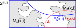
(b) Second counterexample.

Figure 14: Working principle of QbfWin.

Illustration. Figure 14 illustrates the computation of a circuit for one control signal $c_{j}$. The boxes represent the set $2^{|\overline{x}\cup\overline{i}|}$ of all possible assignments to the variables $\overline{x}$ and $\overline{i}$. Figure 14a depicts the initial situation. The region $M_{1}$ represents the set of all situations where $c_{j}$ must be $\mathsf{true}$, and $M_{0}$ represents the situations where $c_{j}$ must be $\mathsf{false}$. The definition of the strategy ensures that these two regions cannot overlap. The current approximation $F_{j}$ of the solution is depicted in blue. Initially, $F_{j}=\mathsf{true}$ (Line 5 in QbfSynt). Next, a counterexample $\mathbf{x},\mathbf{i}\models F_{j}\wedge M_{0}$ is computed (Line 6). It is drawn as a red dot in Figure 14a. The counterexample cube $\mathbf{x}\wedge\mathbf{i}$ is then generalized into a larger region $\mathbf{d}_{g}$ by eliminating literals as long as $\mathbf{d}_{g}$ does not intersect with $M_{1}$. This is ensured by the check in Line 15 of QbfSynt. Next, $F_{j}$ is refined by subtracting the resulting region $\mathbf{d}_{g}$. The refined formula $F_{j}$ is shown as a blue outline Figure 14b. Since the first counterexample is no longer contained in $F_{j}\wedge M_{0}$, it cannot be encountered again. Instead, the algorithm computes a different counterexample, which is generalized in the same way. This is illustrated in Figure 14b. After subtracting the second $\mathbf{d}_{g}$ from $F_{j}$ (which is not shown in Figure 14), $F_{j}$ does not intersect with $M_{0}$ any more. Hence there are no more situations where $F_{j}$ is $\mathsf{true}$ but must be $\mathsf{false}$. Since we did not remove any situation that is contained in $M_{1}$ from $F_{j}$, the final solution satisfies $M_{1}\rightarrow F_{j}\rightarrow\neg M_{0}$ and the while-loop in QbfSynt terminates. That is, $F_{j}$ exploits the freedom between $M_{1}$ and $M_{0}$. Compared to learning a CNF formula for $\neg M_{0}$ precisely, this potentially reduces the number of iterations and the resulting circuit size, especially if $\neg M_{0}$ is complicated. In Figure 14, this is indicated by $M_{0}$ being more irregular in shape than $F_{j}$.

4.2.2 Efficient Implementation for Safety Synthesis Problems

The procedure SafeQbfSynt in Algorithm 13 presents an efficient realization of QbfSynt for the case of safety specifications, where the winning strategy $S(\overline{x},\overline{i},\overline{c},\overline{x}^{\prime})$ is defined via a winning region (or a winning area) $W(\overline{x})$. To make the QBF queries efficient, our aim is to avoid disjunctions and negations of subformulas as much as possible, and to reduce the amount of universal quantification.

Algorithm 13 SafeQbfSynt: Synthesizes circuits from winning areas with QBF-based CNF learning.

1:procedure SafeQbfSynt($T(\overline{x},\overline{i},\overline{c},\overline{x}^{\prime})$, $W(\overline{x})$)

2:   $T^{\prime}(\overline{x},\overline{i},\overline{c},\overline{x}^{\prime}):=T(\overline{x},\overline{i},\overline{c},\overline{x}^{\prime})$,  $\overline{c}_{b}:=\overline{c}$,  $\overline{c}_{a}:=\emptyset$

3:   for all $j$ from $1$ to $|\overline{c}|$ do

4:      $\overline{c}_{b}:=\overline{c}_{b}\setminus\{c_{j}\}$

5:      $M_{1}(\overline{x},\overline{i}):=\forall\overline{c}_{b}\operatorname{\mathbin{:}}\exists\overline{c}_{a},\overline{x}^{\prime}\operatorname{\mathbin{:}}T^{\prime}\bigl{(}\overline{x},\overline{i},\overline{c}_{a},\mathsf{false},\overline{c}_{b},\overline{x}^{\prime}\bigr{)}\wedge W(\overline{x})\wedge\neg W(\overline{x}^{\prime})$

6:      $M_{0}(\overline{x},\overline{i}):=\forall\overline{c}_{b}\operatorname{\mathbin{:}}\exists\overline{c}_{a},\overline{x}^{\prime}\operatorname{\mathbin{:}}T^{\prime}\bigl{(}\overline{x},\overline{i},\overline{c}_{a},\mathsf{true},\overline{c}_{b},\overline{x}^{\prime}\bigr{)}\wedge W(\overline{x})\wedge\neg W(\overline{x}^{\prime})$

7:      $F_{j}(\overline{x},\overline{i}):=\mathsf{true}$

8:      while $\mathsf{sat}$ in $(\mathsf{sat},\mathbf{x},\mathbf{i}):=\textsc{QbfSatModel}\bigl{(}\exists\overline{x},\overline{i}\operatorname{\mathbin{:}}F_{j}(\overline{x},\overline{i})\wedge M_{0}(\overline{x},\overline{i})\bigr{)}$ do

9:         $\mathbf{d}_{g}:=\textsc{QbfGeneralize}\bigl{(}\mathbf{x}\wedge\mathbf{i},M_{1}(\overline{x},\overline{i})\bigr{)}$

10:         $F_{j}(\overline{x},\overline{i}):=F_{j}(\overline{x},\overline{i})\wedge\neg\mathbf{d}_{g}$       

11:      $\textsc{dumpCircuit}\bigl{(}c_{j},F_{j}(\overline{x},\overline{i})\bigr{)}$

12:      $T^{\prime}(\overline{x},\overline{i},\overline{c},\overline{x}^{\prime}):=T^{\prime}(\overline{x},\overline{i},\overline{c},\overline{x}^{\prime})\wedge\bigl{(}c_{j}\leftrightarrow F_{j}(\overline{x},\overline{i})\bigr{)}$

13:      $\overline{c}_{a}:=\overline{c}_{a}\cup\{c_{j}\}$    

14:procedure QbfGeneralize$\left(\mathbf{d},M_{1}(\overline{x},\overline{i})\right)$, returns: $\mathbf{d}_{g}\subseteq\mathbf{d}$ such that $\mathbf{d}_{g}\wedge M_{1}$ is unsatisfiable

15:   $\mathbf{d}_{g}:=\mathbf{x}\wedge\mathbf{i}$

16:   for each literal $l$ in $\mathbf{d}$ do

17:      $\mathbf{d}_{t}:=\mathbf{d}_{g}\setminus\{l\}$

18:      if $\neg\textsc{QbfSatModel}\bigl{(}\exists\overline{x},\overline{i}\operatorname{\mathbin{:}}\mathbf{d}_{t}\wedge M_{1}(\overline{x},\overline{i})\bigr{)}$ then

19:         $\mathbf{d}_{g}:=\mathbf{d}_{t}$          

20:   return $\mathbf{d}_{g}$

Grouping of control variables. In every iteration, SafeQbfSynt splits the control variables $\overline{c}$ into three groups $\overline{c}_{a}$, $c_{j}$, $\overline{c}_{b}$: The single variable $c_{j}$ is the one for which a circuit is constructed in the current iteration, $\overline{c}_{a}$ contains all variables for which a circuit has already been computed, and $\overline{c}_{b}$ contains all control variables for which a circuit will be computed in some future iteration. This split is performed in the Lines 2, 4 and 13, and will allow us to reduce the amount of universal quantification.

Definition of $M_{1}$ and $M_{0}$. With $S(\overline{x},\overline{i},\overline{c},\overline{x}^{\prime})=T(\overline{x},\overline{i},\overline{c},\overline{x}^{\prime})\wedge\bigl{(}\neg W(\overline{x})\vee W(\overline{x}^{\prime})\bigr{)}$, we can apply the following transformations to compute a CNF for $M_{1}$ more efficiently.

$$M_{1}(\overline{x},\overline{i})= \forall\overline{c},\overline{x}^{\prime}\operatorname{\mathbin{:}}\neg S\bigl{(}\overline{x},\overline{i},(c_{0},\ldots,c_{j-1},\mathsf{false},c_{j+1},\ldots,c_{n}),\overline{x}^{\prime}\bigr{)}$$

$$= \forall\overline{c}_{b},\overline{c}_{a},\overline{x}^{\prime}\operatorname{\mathbin{:}}\neg\Bigl{(}T(\overline{x},\overline{i},\overline{c}_{a},\mathsf{false},\overline{c}_{b},\overline{x}^{\prime})\wedge\bigl{(}\neg W(\overline{x})\vee W(\overline{x}^{\prime})\bigr{)}\Bigr{)}$$

$$= \forall\overline{c}_{b},\overline{c}_{a},\overline{x}^{\prime}\operatorname{\mathbin{:}}\Bigl{(}T(\overline{x},\overline{i},\overline{c}_{a},\mathsf{false},\overline{c}_{b},\overline{x}^{\prime})\rightarrow\bigl{(}W(\overline{x})\wedge\neg W(\overline{x}^{\prime})\bigr{)}\Bigr{)}$$

SafeQbfSynt keeps a copy $T^{\prime}$ of the transition relation $T$. It is updated in such a way that the variables $\overline{c}_{a},\overline{x}^{\prime}$ are defined uniquely by $T^{\prime}$. For $\overline{x}^{\prime}$, this holds initially. For $\overline{c}_{a}$, this is ensured by Line 12. Thus, by using $T^{\prime}$ instead of $T$ and applying the one-point rule (2), the universal quantification of $\overline{c}_{a},\overline{x}^{\prime}$ can be turned into an existential one:

$$M_{1}(\overline{x},\overline{i})=\forall\overline{c}_{b}\operatorname{\mathbin{:}}\exists\overline{c}_{a},\overline{x}^{\prime}\operatorname{\mathbin{:}}\Bigl{(}T^{\prime}(\overline{x},\overline{i},\overline{c}_{a},\mathsf{false},\overline{c}_{b},\overline{x}^{\prime})\wedge W(\overline{x})\wedge\neg W(\overline{x}^{\prime})\Bigr{)}$$

The computation of $M_{0}(\overline{x},\overline{i})$ works analogously. As a result, only the control signals $\overline{c}_{b}$, for which no solution has been computed yet, are quantified universally in the QBF queries of Line 8 and 18. The variable vector $\overline{c}_{b}$ becomes shorter from iteration to iteration, which means that the formula gets “more propositional”. In the last iteration, a SAT solver can actually be used instead of a QBF solver.

CNF conversion. The QBF queries in Line 8 and 18 contain only conjunctions. The formula $F_{j}$ is always in CNF. Furthermore, most of our methods to compute a winning region or a winning area produce $W(\overline{x})$ in CNF. Hence, we only need to compute a CNF representation of $T^{\prime}$ and $\neg W(\overline{x}^{\prime})$. NegLearn (Algorithm 11), which negates a formula without introducing auxiliary variables, was beneficial in the QBF certification approach but does not pay off in the learning-based approach. Hence, we apply the method of Plaisted and Greenbaum [31] to compute a CNF for $\neg W(\overline{x}^{\prime})$.

QBF preprocessing. With our extension of Bloqqer [55] to preserve satisfying assignments, QBF preprocessing can be applied both for counterexample computation and generalization. However, while preprocessing was vital in our methods for computing a winning region, it does not give a significant speedup for SafeQbfSynt (see Chapter 5).

Incremental QBF solving. SafeQbfSynt is very well suited for incremental QBF solving, especially with a solver interface such as the one provided by DepQBF [56, 75]. We propose to use two solver instances incrementally. The first instance stores $F_{j}\wedge M_{0}$ and is used for Line 8. Since Line 10 only adds clauses to $F_{j}$, this solver instance is only re-initialized when a mayor iteration (synthesizing the next $c_{j}$) is started. The second solver instance stores $M_{1}$, is used for Line 18, and is also re-initialized when a mayor iteration starts. Before executing the loop in Line 16, we let the second solver instance compute an unsatisfiable core $\mathbf{d}_{g}$ of $\mathbf{d}=\mathbf{x}\wedge\mathbf{i}$ and only reduce this core further in the loop. The conjunction with $\mathbf{d}_{t}$ is realized with assumption literals.

4.2.3 Discussion

Greediness. QbfSynt is greedy in exploiting implementation freedom. When synthesizing a circuit for one control signal $c_{j}$, QbfSynt ensures that some solution for the remaining control signals still exists. However, the algorithm does not specifically attempt to retain implementation freedom for the remaining control signals. This can have the effect that the signals synthesized early have a small implementation, which is found after only a few refinements. Yet, for the signals synthesized later, the implementation freedom may already be “exhausted” and large implementations may be produced after many refinements. Consequently, the performance may also strongly depend on the order in which control signals are processed. This is similar to the standard CofSynt procedure, but different from the QBF certification approach from Section 4.1, which computes circuits for all control signals simultaneously.

Independence of symbolic representation. In contrast to CofSynt and QBF certification, the QBF-based learning approach is rather independent of the symbolic strategy representation and the reasoning engine. Only the concrete counterexamples computed by Line 6 may differ, and our experience in trying to develop heuristics for computing good counterexamples indicates that one counterexample is usually just as good as any other. Consequently, the number of iterations and the resulting circuit will be similar, independent of whether the strategy formula is encoded efficiently or not. When implemented using BDDs, the variable ordering has little impact on these metrics too.

Circuit depth. Another advantage of the QBF-based CNF learning algorithm presented in this section is that the produced circuits have a low depth. This can be an important property because the circuit depth determines the maximum clock frequency with which the circuit can be operated. The formulas $F_{j}$ defining the control signals $c_{j}$ are computed in CNF. When these formulas are transformed into circuits in the straightforward way, this yields circuits with a depth of at most $3$: every signal $\overline{x},\overline{i}$ needs to pass at most one inverter, one OR-gate and one AND-gate. Depending on the gates available in the standard cell library, it may not be feasible to realize the circuit in this straightforward way. However, experiments [61] with a simplistic standard cell library suggest that the circuit depth is usually much lower than when using the standard CofSynt procedure with BDDs.

4.3 Interpolation

Jiang et al. [26] present an interpolation-based approach to synthesize circuits from strategies. Similar to the cofactor-based approach presented in Algorithm 2 and the QBF-based learning approach from Algorithm 12, it computes circuits for one control signal $c_{j}\in\overline{c}$ after the other. However, in contrast to these previous algorithms, the interpolation-based approach avoids quantifier alternations by temporarily considering other control signals for which no circuits have been computed yet as if they were inputs. We will define the approach by Jiang et al. [26] as an algorithm for our setting in Section 4.3.1. After that, we will present optimizations and an efficient realization for safety specifications. In Section 4.4, we will furthermore combine the approach with query learning.

4.3.1 Basic Algorithm

Algorithm 14 InterpolSynt [26]: Synthesizing circuits from strategies using interpolation.

1:procedure InterpolSynt($S(\overline{x},\overline{i},\overline{c},\overline{x}^{\prime})$)

2:   $\overline{c}_{a}:=\overline{c}$,  $\overline{c}_{b}:=\emptyset$

3:   for all $j$ from $|\overline{c}|$ to $1$ do

4:      $\overline{c}_{a}:=\overline{c}_{a}\setminus\{c_{j}\}$

5:      $M_{1}(\overline{x},\overline{i},\overline{c}_{a}):=\bigl{(}\exists\overline{c}_{b},\overline{x}^{\prime}\operatorname{\mathbin{:}}S(\overline{x},\overline{i},\overline{c}_{a},\mathsf{true},\overline{c}_{b},\overline{x}^{\prime})\bigr{)}\wedge\bigl{(}\neg\exists\overline{c}_{b},\overline{x}^{\prime}\operatorname{\mathbin{:}}S(\overline{x},\overline{i},\overline{c}_{a},\mathsf{false},\overline{c}_{b},\overline{x}^{\prime})\bigr{)}$

6:      $M_{0}(\overline{x},\overline{i},\overline{c}_{a}):=\bigl{(}\exists\overline{c}_{b},\overline{x}^{\prime}\operatorname{\mathbin{:}}S(\overline{x},\overline{i},\overline{c}_{a},\mathsf{false},\overline{c}_{b},\overline{x}^{\prime})\bigr{)}\wedge\bigl{(}\neg\exists\overline{c}_{b},\overline{x}^{\prime}\operatorname{\mathbin{:}}S(\overline{x},\overline{i},\overline{c}_{a},\mathsf{true},\overline{c}_{b},\overline{x}^{\prime})\bigr{)}$

7:      $F_{j}(\overline{x},\overline{i},\overline{c}_{a}):=\textsc{Interpol}\bigl{(}M_{1}(\overline{x},\overline{i},\overline{c}_{a}),M_{0}(\overline{x},\overline{i},\overline{c}_{a})\bigr{)}$

8:      $\textsc{dumpCircuit}\bigl{(}c_{j},F_{j}(\overline{x},\overline{i},\overline{c}_{a})\bigr{)}$

9:      $S(\overline{x},\overline{i},\overline{c},\overline{x}^{\prime}):=S(\overline{x},\overline{i},\overline{c},\overline{x}^{\prime})\wedge\bigl{(}c_{j}\leftrightarrow F_{j}(\overline{x},\overline{i},\overline{c}_{a})\bigr{)}$

10:      $\overline{c}_{b}:=\overline{c}_{b}\cup\{c_{j}\}$    

Algorithm 14 illustrates the approach by Jiang et al. [26] in our setting. As before, the input is a strategy formula $S(\overline{x},\overline{i},\overline{c},\overline{x}^{\prime})$. The procedure does not return any result but directly dumps the produced circuits defining $\overline{c}$.

Variable dependencies. Similar to QbfSynt in Algorithm 12, the variables $\overline{c}=(c_{1},\ldots,c_{n})$ are split into three groups $\overline{c}_{a},c_{j},\overline{c}_{b}$. Here, $c_{j}$ is the variable for which a circuit is computed in the current iteration. The algorithm starts with the last control signal $c_{n}$ and proceeds with decreasing indices. Line 10 makes sure that the variable vector $\overline{c}_{b}$ contains all control variables for which a circuit has been computed in some previous iteration. Finally, $\overline{c}_{a}$ contains all control variables for which a circuit needs to be computed in one of the following iterations. The variables in $\overline{c}_{a}$

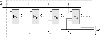
Figure 15: Variable dependencies in interpolation-based circuit synthesis.

are treated as if they were inputs. That is, the circuit defining $c_{j}$ may not only reference variables from $\overline{x}$ and $\overline{i}$, but also all $c_{k}$ with $k<j$ for which no circuit has been computed yet. This is illustrated in Figure 15: $c_{n}$ can also take all signals $c_{1},\ldots,c_{n-1}$ as input, the circuit for $c_{n-1}$ can also take $c_{1},\ldots,c_{n-2}$ as input, etc. Finally, $c_{1}$ cannot depend on any other variables of $\overline{c}$. This ensures that there are no circular dependencies. Furthermore, when the circuits for all $c_{j}\in\overline{c}$ are built together, the signals $\overline{c}$ effectively depend on $\overline{x}$ and $\overline{i}$ only.

Definition of $M_{1}$ and $M_{0}$. Let $\overline{d}=\overline{x}\cup\overline{i}\cup\overline{c}_{a}$ be the vector of all variables on which the current control signal $c_{j}$ may depend. Line 5 of InterpolSynt computes $M_{1}(\overline{d})$, which characterizes the set of all $\overline{d}$-assignments for which $c_{j}$ must be $\mathsf{true}$. This is done as follows. The subformula $C_{1}(\overline{d})=\exists\overline{c}_{b},\overline{x}^{\prime}\operatorname{\mathbin{:}}S(\overline{x},\overline{i},\overline{c}_{a},\mathsf{true},\overline{c}_{b},\overline{x}^{\prime})$ characterizes the set of all $\overline{d}$-assignments for which $c_{j}=\mathsf{true}$ is allowed by $S$. This is essentially the positive cofactor of $S$ regarding $c_{j}$, but the variables $\overline{c}_{b},\overline{x}^{\prime}$ are also quantified existentially, which means that their concrete value is irrelevant as long as some value exists. Similarly, the subformula $C_{0}(\overline{d})=\exists\overline{c}_{b},\overline{x}^{\prime}\operatorname{\mathbin{:}}S(\overline{x},\overline{i},\overline{c}_{a},\mathsf{false},\overline{c}_{b},\overline{x}^{\prime})$ characterizes the set of all $\overline{d}$-assignments for which $c_{j}=\mathsf{false}$ is allowed by $S$. Hence, $M_{1}$ represents the set of all $\overline{d}$-assignments for which $\mathsf{true}$ is allowed, but $\mathsf{false}$ is not allowed. Analogously, Line 6 computes the formula $M_{0}$, which characterizes the $\overline{d}$-assignments for which $c_{j}$ must be $\mathsf{false}$. In principle, $M_{1}$ and $M_{0}$ can easily be transformed into a propositional CNF formula by renaming or expanding the existentially quantified variables. An efficient solution to do so will be presented in Section 4.3.3, but for now we focus on understandability rather than efficiency.

Differences to QbfSynt. Note that the procedure QbfSynt from Algorithm 12 computes $M_{1}$ and $M_{0}$ differently in two respects. First, $M_{1}(\overline{x},\overline{i})$ and $M_{0}(\overline{x},\overline{i})$ do not contain $\overline{c}_{a}$ as free variables in QbfSynt. Second, $M_{1}(\overline{x},\overline{i})$ is computed as $\neg C_{0}(\overline{x},\overline{i})$ in QbfSynt instead of $C_{1}(\overline{d})\wedge\neg C_{0}(\overline{d})$ (and similar for $M_{0}(\overline{x},\overline{i})$). The additional conjunction with $C_{1}(\overline{d})$ in InterpolSynt is necessary for the following reason. We have that $\neg C_{0}(\overline{x},\overline{i})\rightarrow C_{1}(\overline{x},\overline{i})$ and $\neg C_{1}(\overline{x},\overline{i})\rightarrow C_{0}(\overline{x},\overline{i})$ in QbfSynt because $\forall\overline{x},\overline{i}\operatorname{\mathbin{:}}\exists\overline{c},\overline{x}^{\prime}\operatorname{\mathbin{:}}S(\overline{x},\overline{i},\overline{c},\overline{x}^{\prime})$ is guaranteed by the strategy. In other words, for every $(\overline{x},\overline{i})$-assignment, any control signal $c_{j}$ can either be $\mathsf{true}$ or $\mathsf{false}$ (or both). Hence, the additional conjunct $C_{1}(\overline{x},\overline{i})$ would be of no use in $M_{1}(\overline{x},\overline{i})=\neg C_{0}(\overline{x},\overline{i})$ as defined by QbfSynt, because it is implied anyway. Yet, $\neg C_{0}(\overline{d})\rightarrow C_{1}(\overline{d})$ and $\neg C_{1}(\overline{d})\rightarrow C_{0}(\overline{d})$ do not hold in InterpolSynt: there may be $\overline{d}$-assignment for which neither $c_{j}=\mathsf{true}$ nor $c_{j}=\mathsf{false}$ is allowed by the strategy. The reason is that we also consider the signals $\overline{c}_{a}$ as if they were inputs, but $\forall\overline{x},\overline{i},\overline{c}_{a}\operatorname{\mathbin{:}}\exists c_{j},\overline{c}_{b},\overline{x}^{\prime}\operatorname{\mathbin{:}}S(\overline{x},\overline{i},\overline{c}_{a},c_{j},\overline{c}_{b},\overline{x}^{\prime})$ does not hold in general. For $\overline{d}$-assignments for which neither $c_{j}=\mathsf{true}$ nor $c_{j}=\mathsf{false}$ is allowed, the definition of $M_{1}=C_{1}(\overline{d})\wedge\neg C_{0}(\overline{d})$ and $M_{0}=C_{0}(\overline{d})\wedge\neg C_{1}(\overline{d})$ allows both values for $c_{j}$. This is justified by the fact that the circuits synthesized for $\overline{c}_{a}$ in subsequent iterations will make sure that such $\overline{d}$-assignments will never occur as input of the circuit defining $c_{j}$. We refer to Jiang et al. [26] for details on this technical subtlety.

Interpolation. The conjunction $M_{1}(\overline{d})\wedge M_{0}(\overline{d})=C_{1}(\overline{d})\wedge\neg C_{0}(\overline{d})\wedge C_{0}(\overline{d})\wedge\neg C_{1}(\overline{d})$ is trivially unsatisfiable, so an interpolant $F_{j}(\overline{d})$ can be computed in Line 7. The properties of an interpolant (see Section 2.1.1) ensure that $M_{1}\rightarrow F_{j}\rightarrow\neg M_{0}$. The first implication means that $F_{j}$ is $\mathsf{true}$ whenever $c_{j}$ must be $\mathsf{true}$. The second implication means that if $F_{j}$ is $\mathsf{true}$, then $c_{j}$ does not have to $\mathsf{false}$. This means that $F_{j}(\overline{d})$ is a proper implementation for $c_{j}$.

Circuit construction and resubstitution. The remaining steps of the InterpolSynt procedure are the same as for CofSynt (Algorithm 2) and QbfSynt (Algorithm 12). Line 8 constructs a circuit which sets $c_{j}=\mathsf{true}$ if an only if $F_{j}(\overline{x},\overline{i},\overline{c}_{a})$ evaluates to $\mathsf{true}$. Finally, Line 9 refines the strategy formula $S$ with the concrete implementation for $c_{j}$.

Auxiliary variables. If the strategy formula $S$ is defined using auxiliary variables, these can all be put into $\overline{c}_{b}$. This also applies to auxiliary variables that may be introduced in the resubstitution in Line 9.

Variations. Jiang et al. [26] propose to perform a second pass over all control signals, where the circuits for all $c_{j}$ are recomputed using interpolation, while fixing the implementation for the other control signals. This has the potential for producing smaller circuits because the recomputed interpolants can now rely on some concrete realization for the other control signals. However, in preliminary experiments for our setting, this second pass did not result in considerable circuit size improvements (but rather increased the circuit size for many cases). Since such a second pass also increases the computation time, we do not perform it. Jiang et al. [26] also propose a second interpolation-based approach which does not treat other control signals as if they were inputs but rather quantifies them universally and applies universal expansion to eliminate the quantifiers. However, this can blow up the formula size significantly. Preliminary experiments with this second approach were not promising in our setting either.

4.3.2 Dependency Optimization

For some specifications, the performance of InterpolSynt strongly depends on the order in which the control signals $\overline{c}=(c_{1},\ldots,c_{n})$ are processed. One reason is that this order defines which signal $c_{j}$ may depend on which other signals $c_{k}$. The aim of the optimization presented in this section is to increase the set of variables on which a certain signal $c_{j}$ can depend. This increases the freedom for the interpolation procedure (the interpolant $F_{j}$ may still choose the ignore the additional signals) and can lead to smaller interpolants and shorter execution times.

Basic idea. The basic idea is as follows. As illustrated in Figure 15, the interpolant $F_{n}$ computed first can reference all other control signals $c_{1},\ldots,c_{n-1}$. The interpolant $F_{n-1}$ computed in the second iteration cannot depend on $c_{n}$, though. The reason is that $F_{n}$, which defines $c_{n}$, could in turn reference $c_{n-1}$, which would result in a circular dependency. Yet, the concrete interpolant $F_{n}$ may choose to ignore $c_{n-1}$ completely. In this case, $F_{n-1}$ can in fact be allowed to reference $c_{n}$. The reason is that there is no danger to introduce a circular dependency — the result would be the same as if $c_{n}$ and $c_{n-1}$ would have been processed by InterpolSynt in reverse order.

Realization. In the iteration synthesizing a solution for $c_{j}$, we analyze which other signals $c_{k}$ with $k>j$ do not transitively depend on $c_{j}$. This is done on a syntactic level by checking if $c_{j}$ occurs in the fan-in cone of $c_{k}$ when the circuits for $F_{j+1},\ldots,F_{n}$ are combined. If $c_{j}$ does not appear in the fan-in cone of $c_{k}$, then $c_{k}$ is moved (temporarily) from $\overline{c}_{b}$ to $\overline{c}_{a}$. Thus, $F_{j}(\overline{x},\overline{i},\overline{c}_{a})$ can reference $c_{k}$.

Dependencies on auxiliary variables. Depending on the realization of Interpol, the computed interpolants $F_{j}(\overline{x},\overline{i},\overline{c}_{a})$ may be represented using auxiliary variables (e.g., introduced by a Tseitin-transformation [30]) that act as abbreviation for some subformulas over $\overline{x}$, $\overline{i}$ and $\overline{c}_{a}$. As mentioned in the previous subsection, all auxiliary variables are put into $\overline{c}_{b}$, so they cannot be referenced by the computed interpolants by default. However, the dependency analysis cannot only be performed for the final output of each $F_{k}$ with $k>j$, but also on their auxiliary variables: if the current $c_{j}$ does not appear in the fan-in cone of some auxiliary variable $t$, then $t$ can be moved from $\overline{c}_{b}$ to $\overline{c}_{a}$.

4.3.3 Efficient Implementation for Safety Synthesis Problems

The procedure SafeInterpolSynt in Algorithm 15 shows an efficient implementation of InterpolSynt if the winning strategy is defined via a winning region (or winning area) $W(\overline{x})$ of a safety specification. The dependency optimization is not included for the sake of readability.

Algorithm 15 SafeInterpolSynt: Synthesizing circuits from winning areas using interpolation.

1:procedure SafeInterpolSynt($T(\overline{x},\overline{i},\overline{c},\overline{x}^{\prime})$, $W(\overline{x})$)

2:   $T^{\prime}(\overline{x},\overline{i},\overline{c},\overline{x}^{\prime}):=T(\overline{x},\overline{i},\overline{c},\overline{x}^{\prime})$,  $\overline{c}_{a}:=\overline{c}$,  $\overline{c}_{b}:=\emptyset$

3:   for all $j$ from $|\overline{c}|$ to $1$ do

4:      $\overline{c}_{a}:=\overline{c}_{a}\setminus\{c_{j}\}$

5:      $\overline{c}_{b1},\overline{c}_{b2},\overline{c}_{b3},\overline{c}_{b4}:=\textsf{create4FreshCopies}(\overline{c}_{b})$

6:      $\overline{x}_{1}^{\prime},\,\overline{x}_{2}^{\prime},\,\overline{x}_{3}^{\prime},\,\overline{x}_{4}^{\prime}\,\,:=\textsf{create4FreshCopies}(\overline{x}^{\prime})$

7:      $M_{1}^{\prime}(\overline{x},\overline{i},\overline{c}_{a},\overline{c}_{b1},\overline{c}_{b2},\overline{x}_{1}^{\prime},\overline{x}_{2}^{\prime}):=T^{\prime}(\overline{x},\overline{i},\overline{c}_{a},\mathsf{true},\overline{c}_{b1},\overline{x}_{1}^{\prime})\wedge W(\overline{x}_{1}^{\prime})\wedge T^{\prime}(\overline{x},\overline{i},\overline{c}_{a},\mathsf{false},\overline{c}_{b2},\overline{x}_{2}^{\prime})\wedge W(\overline{x})\wedge\neg W(\overline{x}_{2}^{\prime})$

8:      $M_{0}^{\prime}(\overline{x},\overline{i},\overline{c}_{a},\overline{c}_{b3},\overline{c}_{b4},\overline{x}_{3}^{\prime},\overline{x}_{4}^{\prime}):=T^{\prime}(\overline{x},\overline{i},\overline{c}_{a},\mathsf{false},\overline{c}_{b3},\overline{x}_{3}^{\prime})\wedge W(\overline{x}_{3}^{\prime})\wedge T^{\prime}(\overline{x},\overline{i},\overline{c}_{a},\mathsf{true},\overline{c}_{b4},\overline{x}_{4}^{\prime})\wedge W(\overline{x})\wedge\neg W(\overline{x}_{4}^{\prime})$

9:      $F_{j}(\overline{x},\overline{i},\overline{c}_{a}):=\textsc{Interpol}\bigl{(}M_{1}^{\prime}(\overline{x},\overline{i},\overline{c}_{a},\overline{c}_{b1},\overline{c}_{b2},\overline{x}_{1}^{\prime},\overline{x}_{2}^{\prime}),M_{0}^{\prime}(\overline{x},\overline{i},\overline{c}_{a},\overline{c}_{b3},\overline{c}_{b4},\overline{x}_{3}^{\prime},\overline{x}_{4}^{\prime})\bigr{)}$

10:      $\textsc{dumpCircuit}\bigl{(}c_{j},F_{j}(\overline{x},\overline{i},\overline{c}_{a})\bigr{)}$

11:      $T^{\prime}(\overline{x},\overline{i},\overline{c},\overline{x}^{\prime}):=T^{\prime}(\overline{x},\overline{i},\overline{c},\overline{x}^{\prime})\wedge\bigl{(}c_{j}\leftrightarrow F_{j}(\overline{x},\overline{i},\overline{c}_{a})\bigr{)}$

12:      $\overline{c}_{b}:=\overline{c}_{b}\cup\{c_{j}\}$    

Computation of $M_{1}$ and $M_{0}$. With $S(\overline{x},\overline{i},\overline{c},\overline{x}^{\prime})=T(\overline{x},\overline{i},\overline{c},\overline{x}^{\prime})\wedge\bigl{(}\neg W(\overline{x})\vee W(\overline{x}^{\prime})\bigr{)}$, we can apply the following transformations to compute a more compact CNF for $M_{1}$ as $M_{1}(\overline{x},\overline{i},\overline{c}_{a})=$

$$\;\bigl{(}\exists\overline{c}_{b},\overline{x}^{\prime}\operatorname{\mathbin{:}}S(\overline{x},\overline{i},\overline{c}_{a},\mathsf{true},\overline{c}_{b},\overline{x}^{\prime})\bigr{)}\wedge\bigl{(}\neg\exists\overline{c}_{b},\overline{x}^{\prime}\operatorname{\mathbin{:}}S(\overline{x},\overline{i},\overline{c}_{a},\mathsf{false},\overline{c}_{b},\overline{x}^{\prime})\bigr{)}$$

$$= \;\Bigl{(}\exists\overline{c}_{b},\overline{x}^{\prime}\operatorname{\mathbin{:}}T(\overline{x},\overline{i},\overline{c}_{a},\mathsf{true},\overline{c}_{b},\overline{x}^{\prime})\wedge\bigl{(}\neg W(\overline{x})\vee W(\overline{x}^{\prime})\bigr{)}\Bigr{)}\wedge\Bigl{(}\neg\exists\overline{c}_{b},\overline{x}^{\prime}\operatorname{\mathbin{:}}T(\overline{x},\overline{i},\overline{c}_{a},\mathsf{false},\overline{c}_{b},\overline{x}^{\prime})\wedge\bigl{(}\neg W(\overline{x})\vee W(\overline{x}^{\prime})\bigr{)}\Bigr{)}$$

$$= \;\Bigl{(}\exists\overline{c}_{b},\overline{x}^{\prime}\operatorname{\mathbin{:}}T(\overline{x},\overline{i},\overline{c}_{a},\mathsf{true},\overline{c}_{b},\overline{x}^{\prime})\wedge\bigl{(}\neg W(\overline{x})\vee W(\overline{x}^{\prime})\bigr{)}\Bigr{)}\wedge\Bigl{(}\forall\overline{c}_{b},\overline{x}^{\prime}\operatorname{\mathbin{:}}T(\overline{x},\overline{i},\overline{c}_{a},\mathsf{false},\overline{c}_{b},\overline{x}^{\prime})\rightarrow\bigl{(}W(\overline{x})\wedge\neg W(\overline{x}^{\prime})\bigr{)}\Bigr{)}$$

That is, the negation turns the existential quantification over $\overline{c}_{b},\overline{x}^{\prime}$ into a universal one. Yet, just like SafeQbfSynt (Algorithm 13), SafeInterpolSynt also keeps a copy $T^{\prime}$ of the transition relation $T$ that defines all variables in $\overline{c}_{b}$ and $\overline{x}^{\prime}$ uniquely based on the other variables. For the variables $\overline{x}^{\prime}$, this holds initially. For $\overline{c}_{b}$, this is ensured by Line 11. Thus, by using $T^{\prime}$ instead of $T$ and by applying the one-point rule (2), the universal quantification can be turned into an existential one:

$$\Bigl{(}\exists\overline{c}_{b},\overline{x}^{\prime}\operatorname{\mathbin{:}}T^{\prime}(\overline{x},\overline{i},\overline{c}_{a},\mathsf{true},\overline{c}_{b},\overline{x}^{\prime})\wedge\bigl{(}\neg W(\overline{x})\vee W(\overline{x}^{\prime})\bigr{)}\Bigr{)}\wedge\Bigl{(}\exists\overline{c}_{b},\overline{x}^{\prime}\operatorname{\mathbin{:}}T^{\prime}(\overline{x},\overline{i},\overline{c}_{a},\mathsf{false},\overline{c}_{b},\overline{x}^{\prime})\wedge W(\overline{x})\wedge\neg W(\overline{x}^{\prime})\Bigr{)}$$

By renaming the variables $\overline{c}_{b}$ and $\overline{x}^{\prime}$, the two subformulas can be merged into one block of quantifiers:

$$\exists\overline{c}_{b1},\overline{c}_{b2},\overline{x}_{1}^{\prime},\overline{x}_{2}^{\prime}\operatorname{\mathbin{:}}T^{\prime}(\overline{x},\overline{i},\overline{c}_{a},\mathsf{true},\overline{c}_{b1},\overline{x}_{1}^{\prime})\wedge\bigl{(}\neg W(\overline{x})\vee W(\overline{x}_{1}^{\prime})\bigr{)}\wedge T^{\prime}(\overline{x},\overline{i},\overline{c}_{a},\mathsf{false},\overline{c}_{b2},\overline{x}_{2}^{\prime})\wedge W(\overline{x})\wedge\neg W(\overline{x}_{2}^{\prime})$$

Finally, $\bigl{(}\neg W(\overline{x})\vee W(\overline{x}_{1}^{\prime})\bigr{)}\wedge W(\overline{x})$ can be simplified to $W(\overline{x})\wedge W(\overline{x}_{1}^{\prime})$, which is fortunate because negations and disjunctions are expensive to perform in CNF. This gives

$$M_{1}(\overline{x},\overline{i},\overline{c}_{a})=\exists\overline{c}_{b1},\overline{c}_{b2},\overline{x}_{1}^{\prime},\overline{x}_{2}^{\prime}\operatorname{\mathbin{:}}T^{\prime}(\overline{x},\overline{i},\overline{c}_{a},\mathsf{true},\overline{c}_{b1},\overline{x}_{1}^{\prime})\wedge W(\overline{x}_{1}^{\prime})\wedge T^{\prime}(\overline{x},\overline{i},\overline{c}_{a},\mathsf{false},\overline{c}_{b2},\overline{x}_{2}^{\prime})\wedge W(\overline{x})\wedge\neg W(\overline{x}_{2}^{\prime}).$$

In SafeInterpolSynt, the existential quantification is not applied. Instead, the variables $\overline{c}_{b1}$, $\overline{c}_{b2}$, $\overline{x}_{1}^{\prime}$, $\overline{x}_{2}^{\prime}$ occur freely in $M_{1}^{\prime}$. Similarly, other fresh copies $\overline{c}_{b3},\overline{c}_{b4},\overline{x}_{3}^{\prime},\overline{x}_{4}^{\prime}$ of the same variables occur freely in $M_{0}^{\prime}$. The properties of an interpolant (see Section 2.1.1) ensure that $F_{j}$, computed in Line 9, can only reference the variables $\overline{x},\overline{i},\overline{c}_{a}$ occurring both in $M_{1}^{\prime}$ and in $M_{0}^{\prime}$. Hence, these free variables cannot be referenced in the resulting circuit.

CNF conversion. The formulas in Line 7 and 8 contain only conjunctions. Most of our methods to compute a winning region or a winning area produce $W(\overline{x})$ in CNF. Hence, just as for QBF certification and QBF-based CNF learning, we only need to compute a CNF representation of $T^{\prime}$ and $\neg W(\overline{x}^{\prime})$.

Simplification of interpolants. The computed interpolants $F_{j}$ refine $T^{\prime}$ in Line 11. Hence, complicated representations of $F_{j}$ result in more complicated formulas for $T^{\prime}$, which can increase the time for interpolation (and may result in even more complicated formulas for the subsequent interpolants). Besides optimizing the final circuit regarding size, we therefore also optimize every single interpolant using the tool ABC [67] after it has been computed.

4.3.4 Discussion

Exploiting implementation freedom. InterpolSynt is rather conservative in exploiting implementation freedom when computing a circuit for some control signal $c_{j}$: to the extend where this is feasible, the circuit $F_{j}$ defining $c_{j}$ will work for any realization of the control signals $\overline{c}_{a}$ that have not been synthesized yet. The reason is that the variables of $\overline{c}_{a}$ are handled as if they were inputs. This stands in contrast to QbfSynt, which is more greedy by exploiting implementation freedom as long as some solution for the other signals still exists. Both strategies have their advantages. Preserving implementation freedom can result in smaller circuits for control signals that are synthesized later. The greedy strategy can be better in preventing that implementation freedom is left unexploited.

Dependencies between control signals. In contrast to CofSynt and QbfSynt, InterpolSynt constructs a circuit in such a way that the implementation for one control signal can be reused in the definition of others (see Figure 15). This can result in a smaller total circuit size. As an extreme example, one control signal $c_{j}$ could be required to be an exact copy of some other control signal $c_{k}$. While InterpolSynt may find the implementation $c_{j}=c_{k}$ quickly, both CofSynt and QbfSynt would have to construct the same (potentially complicated) circuit based on the variables $\overline{x}$ and $\overline{i}$ twice. The circuit optimization techniques we apply as a postprocessing step may optimize one copy away, so the final circuit may actually be the same. Nevertheless, computing the same circuit twice is at least a waste of resources.

Dependence on the interpolation procedure. With InterpolSynt, the size of the resulting circuits strongly depends on the ability of the interpolation procedure Interpol to exploit the freedom between $M_{1}$ and $\neg M_{0}$. When the interpolant is computed from an unsatisfiability proof returned by a SAT solver, we must rely on the heuristics in the solver to yield a compact proof that can be used to derive a simple interpolant, which can then be implemented in a small circuit. In contrast, QbfSynt is more independent of the underlying reasoning engine. The next section will present an approach to reduce this dependency of InterpolSynt on the underlying solver.

4.4 Query Learning Based on SAT Solving

In this section, we combine query learning with the idea by Jiang et al. [26] to temporarily treat control signals as if they were inputs. This eliminates the need for universal quantification and allows us to implement the query learning approach from Section 4.2 with a SAT solver instead of a QBF solver. In the following subsection, we will present a solution based on CNF learning. Applying other learning algorithms from [61] publication is possible, but imposes more overhead for encoding formula parts into CNF. After introducing the basic algorithm, we will again present an efficient realization for safety synthesis problems and discuss the differences to the other algorithms.

4.4.1 CNF Learning Based on SAT Solving

In Section 4.2, we have discussed that query learning can be used as a special interpolation procedure if different formulas are used for counterexample computation and generalization. While Section 4.2 used this idea to compute interpolants between quantified formulas using a QBF solver, we use it here to compute interpolants for propositional formulas using CNF learning.

Algorithm 16 CnfInterpol: Computing an interpolant using CNF learning with a SAT solver.

1:procedure CnfInterpol$\left(M_{1}(\overline{d},\overline{t}_{1}),M_{0}(\overline{d},\overline{t}_{0})\right)$,                     returns: A CNF $F(\overline{d})$ with $M_{1}\rightarrow F\rightarrow\neg M_{0}$

2:   $F(\overline{d}):=\mathsf{true}$

3:   while $\mathsf{sat}$ in $(\mathsf{sat},\mathbf{d}):=\textsc{PropSatModel}\bigl{(}M_{0}(\overline{d},\overline{t}_{0})\wedge F(\overline{d})\bigr{)}$ do

4:      $F(\overline{d}):=F(\overline{d})\wedge\neg\textsc{PropMinUnsatCore}\bigl{(}\mathbf{d},M_{1}(\overline{d},\overline{t}_{1})\bigr{)}$    

5:   return $F(\overline{d})$

Algorithm. We keep the basic structure of the InterpolSynt procedure from Algorithm 14, but replace the call to Interpol in Line 7 by a call to CnfInterpol, which is defined in Algorithm 16. The interface of CnfInterpol is the same as that of any interpolation procedure: given two formulas $M_{1}(\overline{d},\overline{t}_{1})$ and $M_{0}(\overline{d},\overline{t}_{0})$ such that $M_{1}\wedge M_{0}$ is unsatisfiable, it returns a formula $F(\overline{d})$ over the shared variables $\overline{d}$ such that $M_{1}\rightarrow F\rightarrow\neg M_{0}$. The implementation of CnfInterpol is simple. It starts with the initial approximation $F=\mathsf{true}$ and enforces the invariant $M_{1}\rightarrow F$. Line 3 checks if $F\rightarrow\neg M_{0}$, which is the case if and only if $F\wedge M_{0}$ is unsatisfiable. If so, then $M_{1}\rightarrow F\rightarrow\neg M_{0}$ holds, so the loop terminates and $F$ is returned as result. Otherwise a counterexample $\mathbf{d}\models F\wedge M_{0}$ is extracted for which $F$ is $\mathsf{true}$ but must be $\mathsf{false}$. The computation of the unsatisfiable core in Line 4 generalizes the cube $\mathbf{d}$ by dropping literals as long as $\mathbf{d}$ does not intersect with $M_{1}$. Consequently, the update of $F$ in Line 4 preserves the invariant $M_{1}\rightarrow F$ and resolves the counterexample.

Exploiting freedom. As in QbfSynt (Algorithm 12) using $M_{0}$ in counterexample computation makes sure that refinements of $F$ are only triggered if some $\overline{d}$-assignment $\mathbf{d}$ must be mapped to $\mathsf{false}$. Using $M_{1}$ in counterexample generalization entails that other $\overline{d}$-assignments are also mapped to $\mathsf{false}$ as long as they can be mapped to $\mathsf{false}$. Using “can” instead of “must” during generalization potentially eliminates more counterexamples before they are actually encountered by Line 3.

4.4.2 Efficient Implementation for Safety Synthesis Problems

Following the transformations presented for SafeInterpolSynt in Section 4.3.3, CnfInterpol is called with

$$M_{1}(\overline{x},\overline{i},\overline{c}_{a},\overline{c}_{b1},\overline{c}_{b2},\overline{x}_{1}^{\prime},\overline{x}_{2}^{\prime})=T^{\prime}(\overline{x},\overline{i},\overline{c}_{a},\mathsf{true},\overline{c}_{b1},\overline{x}_{1}^{\prime})\wedge W(\overline{x}_{1}^{\prime})\wedge T^{\prime}(\overline{x},\overline{i},\overline{c}_{a},\mathsf{false},\overline{c}_{b2},\overline{x}_{2}^{\prime})\wedge W(\overline{x})\wedge\neg W(\overline{x}_{2}^{\prime})\text{ and}$$

$$M_{0}(\overline{x},\overline{i},\overline{c}_{a},\overline{c}_{b3},\overline{c}_{b4},\overline{x}_{3}^{\prime},\overline{x}_{4}^{\prime})=T^{\prime}(\overline{x},\overline{i},\overline{c}_{a},\mathsf{false},\overline{c}_{b3},\overline{x}_{3}^{\prime})\wedge W(\overline{x}_{3}^{\prime})\wedge T^{\prime}(\overline{x},\overline{i},\overline{c}_{a},\mathsf{true},\overline{c}_{b4},\overline{x}_{4}^{\prime})\wedge W(\overline{x})\wedge\neg W(\overline{x}_{4}^{\prime}).$$

Since CnfInterpol does not perform any negations nor disjunctions, only $\neg W(\overline{x}^{\prime})$ needs to be transformed into CNF.

Dependency optimization. We can apply the dependency optimization presented in Section 4.3.2. However, on top of allowing dependencies on other control signals, we also allow dependencies on auxiliary variables that are used for defining the transition relation $T^{\prime}$ as long as this does not result in circular dependencies.

Incremental solving. CnfInterpol is well suited for incremental SAT solving. A simple solution uses two solver instances, which are initialized whenever CnfInterpol is called. The first solver instance stores $M_{0}\wedge F$ and is used for Line 3. The second one stores $M_{1}$ and is used for Line 4. A more radical solution uses only one solver instance throughout all calls to CnfInterpol. Note that $M_{1}$ differs from $M_{0}$ only by having $c_{j}$ (in two copies) set to different truth constants. Hence, switching between $M_{1}$ and $M_{0}$ can be achieved by setting (the two copies of) $c_{j}$ differently with assumption literals. Furthermore, the clauses of some $F_{j}$ are all disjoined with some fresh activation variable $a_{j}$ before they are asserted in the solver. This way, $F_{j}$ can be enabled or disabled by setting the assumption literal $\neg a_{j}$ or $a_{j}$, respectively. Finally, $T^{\prime}$ changes between major iterations of SafeInterpolSynt (see Line 11). However, additional constraints are only added in this update, so this does not pose any challenge for incremental solving.

Minimizing the final solution. Recall from the interpolation-based method from Section 4.3 that a second pass over all control signals can be performed, in which the circuits for all $c_{j}$ are recomputed while the implementation for the other control signals is fixed. In principle, this has the potential for reducing the circuit size because the recomputed circuits can now rely on some concrete realization for the other control signals. The same idea can also be applied in our SAT solver based CNF learning approach. However, similar to interpolation, recomputing individual circuits by learning them from scratch did not result in circuit size reductions, but more often in circuit size increases in our experiments. Yet, instead of recomputing a circuit from scratch, we can also start with the existing solution $F_{j}$, which is given as a CNF formula, and simplify it by dropping literals and clauses as long as correctness is still preserved. The idea is similar to CompressCnf (Algorithm 7), but the simplification is not equivalence preserving but only correctness preserving. We propose to postprocess all $F_{j}$ in the order of decreasing $j$. The reason is that $F_{n}$ was computed first, without any knowledge about the implementation of the other $F_{j}$. Hence, intuitively, $F_{n}$ has the greatest potential for simplifications relying on the concrete realization of all other $F_{j}$. Each $F_{j}$ satisfies $M_{1}\rightarrow F_{j}\rightarrow\neg M_{0}$ initially, where $M_{1}$ and $M_{0}$ are now defined using the concrete implementation for the other $F_{k}$. We propose to simplify each $F_{j}$ in two phases. The first phase drops literals from clauses of $F_{j}$ as long as $M_{1}\rightarrow F_{j}$ is preserved (because dropping literals can make $F_{j}$ only stronger). Similar to CompressCnf, this can be realized by computing unsatisfiable cores, utilizing incremental SAT solving. The second phase drops clauses from $F_{j}$, starting with the longest ones, as long as $F_{j}\rightarrow\neg M_{0}$ is preserved (because dropping clauses can make $F_{j}$ only weaker). Since we only drop literals and clauses from the existing implementations, this postprocessing can only make the resulting circuits smaller but never larger.

4.4.3 Discussion

The SAT solver based CNF learning approach is very similar to the interpolation-based method from the previous section, and thus inherits most of its strength and weaknesses. However, using the learning algorithm instead of interpolation makes the approach less dependent on the underlying solver. This is similar to QbfSynt. Also similar to QbfSynt is the fact that individual circuits are computed as formulas in CNF. However, because the individual circuits are cascaded as illustrated in Figure 15, the final circuit depth will in general be higher than that of circuits produced by QbfSynt. Still, the circuit depths can be expected to be lower compared to InterpolSynt in most cases. The reason is that interpolants derived from an unsatisfiability proof can have a depth that is much higher than $3$, and the procedure for building the individual circuits together is the same.

4.5 Parallelization

We have already discussed that different methods for circuit synthesis have different characteristics. The experimental results in Chapter 5 will indicate that this results in different methods and optimizations performing well on different classes of benchmarks. Similar to strategy computation (see Section 3.7) we thus propose a parallelization that executes different methods and optimizations in different threads. The aim is to combine the strengths and compensate the weaknesses of the individual methods.

Realization. In contrast to Section 3.7, our parallelization for synthesizing circuits from strategies follows a rather simple portfolio approach, where each thread solves the circuit synthesis problem without any information from other threads. The first thread implements the SAT solver based learning algorithm from Section 4.4 with the dependency optimization from Section 4.3.2. If our parallelization is executed with two threads, the second thread performs QBF-based CNF learning (Section 4.2) with incremental QBF solving. If executed with three threads, the third thread again performs learning using a SAT solver, but without the dependency optimization.

Heuristics. In order to achieve a good balance between low execution time and small circuits, the user can inform our parallelization about a timeout. A heuristic then uses this information to decide whether to perform a minimization of the final solution, as explained in Section 4.4.2, or not. Furthermore, if one thread finishes, it does not stop the other threads immediately but only if the user-defined timeout is approaching or the ratio between waiting time and working time exceeds a certain threshold ($0.25$ in our experiments). The reason is that, from all threads that terminated, we finally select the circuit with the lowest number of gates. Hence, even if one thread has already found a solution, waiting for other threads to finish their computation can be beneficial for the final circuit size.

Alternatives. As for strategy computation, there is a plethora of possibilities to combine different methods while sharing information in a more fine-grained way. Since most of the methods compute circuits for one control signal after the other, the final solutions for each control signal can be exchanged. Each thread can then continue with the smallest solution that has been found for the respective signal. Since several methods are based on counterexample-guided refinements of solution candidates, the respective threads can also exchange counterexamples and the corresponding blocking clauses. Furthermore, it can be beneficial to have different threads synthesizing circuits for control signals in different order. We leave an exploration of such fine-grained parallelization approaches for future work.

5 Experimental Results

In this section, we will first sketch our implementation of the SAT-based synthesis algorithms introduced so far. After that, we will describe benchmarks that will be used in our experimental evaluation (Section 5.2). The core of this section is formed by our performance evaluation for computing strategies (Section 5.3) and for constructing circuits from strategies (Section 5.4). The section concludes with a discussion of the central results (Section 5.5).

5.1 Implementation

We have implemented the synthesis methods presented in Chapter 3 and Chapter 4 in a synthesis tool called Demiurge. It is written in C++ and compatible with the rules for the SyntComp [21] synthesis competition. Demiurge has won two gold medals in this synthesis competition: one in 2014 and one in 2015, both in the parallel synthesis track. The input of Demiurge is a safety specification in AIGER format. The synthesis result is a circuit in AIGER format as well. Since the synthesis process does not involve any interaction with the user except for setting parameters, Demiurge does not come with a GUI, but is started from the command-line. So far, our synthesis tool has only been tested on Linux operating systems. Demiurge is freely available under the GNU Lesser General Public License version 3, and can be downloaded from

https://www.iaik.tugraz.at/content/research/opensource/demiurge/.

All experiments presented in this article have been performed using version 1.2.0. The downloadable archive contains all scripts to reproduce the experiments, as well as spreadsheets with more detailed data (such as execution times for individual steps of the algorithms, numbers of iterations, etc.).

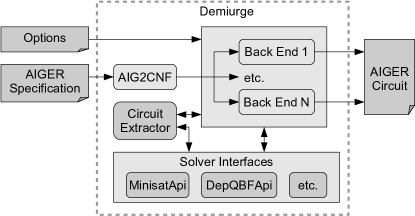
Figure 16: Architecture of the SAT-based synthesis tool Demiurge.

Architecture. The architecture of Demiurge is outlined in Figure 16. The AIG2CNF module parses the specification into CNF formulas representing the transition relation $T$ and the set of safe states $P$. Only one initial state is allowed in the input format, so the initial states $I$ in our definition of a safety specification are represented as a minterm. Next, the back end selected by the user via command-line options is executed. The back ends mostly differ in their method for computing the winning region (or a winning area), and can be parameterized with a method for computing the circuit from the induced winning strategy. Furthermore, the back ends can be configured with options to enable or disable optimizations or optional steps. The back ends can access a number of different solvers via uniform interfaces. That is, multiple SAT solvers can be accessed via the same abstract interface, which hides the concrete solver from the application. Various QBF solvers are accessible via a second interface (which is similar to the interface for SAT solvers). The concrete solvers that shall be used are again configured via command-line options. Due to this extensible architecture, Demiurge can also be seen as a framework for implementing new synthesis algorithms or optimizations with low effort: A lot of infrastructure such as the parser, interfaces to solvers and entire synthesis steps (like computing a circuit from a strategy) can be reused.

External tools. In version 1.2.0, Demiurge has interfaces to

• the SAT solver MiniSat [76] in version 2.2.0 via its API,

• the SAT solver PicoSAT [77] in version 960 via its API,

• the SAT solver Lingeling [78] in version ayv via its API,

• the QBF solver DepQBF [48, 75] in version 3.04 via its API, both with and without preprocessing by Bloqqer [51, 55] version 34,

• the QBF solver RAReQS [50] in version 1.1 via a self-made API,

• the QBF solver QuBE [52] in version 7.2 with communication via files,

• the tool ABC [67] (commit d3db71b) for optimizing AIGER circuits with communication via files, and

• the first-order theorem prover iProver [59] in version 1.0 with communication via files.

5.2 Benchmarks

Table 1: Summary of benchmark sizes. The suffix k multiplies by 1000. The suffix M multiplies by one million.

Name	parameter range	$|\overline{x}|$	$|\overline{i}|$	$|\overline{c}|$	Gates defining $T$
add$ko$	$k=2$ to $20$	$2$	$2\cdot k$	$k$	$17$ to $365$
mult$k$	$k=2$ to $16$	$0$	$2\cdot k$	$2\cdot k$	$24$ to $2450$
cnt$ko$	$k=2$ to $30$	$k+1$	$1$	$1$	$11$ to $450$
mv$ko$	$k=2$ to $28$	$k+1$	$k-1$	$k-1$	$10$ to $469$
bs$ko$	$k=8$ to $128$	$k+1$	$\operatorname{ld}(k)$	$1$	$80$ to $3202$
stay$ko$	$k=2$ to $24$	$k+2$	$k$	$k+1$	$17$ to $4104$
amba$kl$	$k=2$ to $10$	$28$ to $76$	$2\cdot k+3$	$8$ to $19$	$177$ to $630$
genbuf$kl$	$k=1$ to $16$	$21$ to $73$	$k+4$	$6$ to $24$	$134$ to $733$
fact$mnkc$	special selection	$20$ to $54$	$10$ to $40$	$8$ to $12$	$122$ to $594$
mov$klm$	$k=l=8$ to $128$	$19$ to $41$	$12$ to $34$	$5$	$306$ to $830$
driver$kl$	$l=5$ to $8$	$55$ to $326$	$16$ to $98$	$24$ to $82$	$435$ to $1942$
demo$kl$	$k=1$ to $25$	$12$ to $280$	$1$ to $4$	$1$ to $4$	$43$ to $2055$
gb$k$	$k=1$ to $4$	$11$k to $23$k	$4$	$4$	$867$k to $1.7$M
load$kl$	$k=2$ to $3$	$96$ to $296$	$3$ to $4$	$2$ to $3$	$1092$ to $3156$
ltl2dba$kl$	$k=1$ to $20$	$44$ to $484$	$2$ to $7$	$1$	$194$ to $5482$
ltl2dpa$k$	$k=1$ to $18$	$44$ to $340$	$1$ to $3$	$2$ to $4$	$191$ to $3866$

We used benchmarks from the SyntComp 2014 [21] benchmark set to evaluate the performance of our different methods to compute strategies as well as circuits implementing these strategies. Most of the benchmarks are parameterized. In the following, we briefly summarize their main characteristics as far as this is helpful for interpreting the performance results. The size of the benchmarks is summarized in Table 1. All in all, we included $350$ benchmark instances, of which $40$ instances are unrealizable.

The add$ko$ benchmark specifies a combinational adder for two $k$-bit numbers. The parameter $o\in\{\texttt{y},\texttt{n}\}$ indicates if the benchmark file has been optimized with ABC [67] for circuit size (value y) or not (value n). This benchmarks is realizable. Since it is mostly combinational, it challenges circuit synthesis more than strategy computation.

The mult$k$ benchmark specifies a combinational multiplier for two $k$-bit numbers and is thus similar to add.

The cnt$ko$ benchmark specifies a $k$-bit counter that must not reach its maximum value. At value $2^{k-1}-1$, the counter can be reset if the only control signal is set to $\mathsf{true}$. The parameter $o\in\{\texttt{y},\texttt{n}\}$ again indicates if the benchmark was optimized. This benchmark is realizable and can be challenging for strategy computation because it may require many iterations to find the winning region. It is trivial for circuit synthesis, though, because hardwiring the only control signal to $\mathsf{true}$ suffices.

The mv$ko$ benchmark also contains a $k$-bit counter that must not reach its maximum value. However, when the most significant counter bit is set, the counter can be reset if the XOR sum of all control signals is $\mathsf{true}$. Hence, there exists an implementation that hardwires all control signals to constant values. Again, $o\in\{\texttt{y},\texttt{n}\}$ indicates if the benchmark was optimized. The benchmark is realizable and can be challenging for circuit synthesis because it contains many interdependent control signals.

The realizable benchmark bs$ko$ applies a barrel shifter to a $k$-bit register, which is initialized to some constant value and must never reach specific values. The amount of shifting is defined by uncontrollable inputs, but the shifting can be disabled with a control signal. Barrel shifters can be particularly challenging for BDDs.

The benchmark stay$ko$ again contains a $k$-bit counter that must not reach its maximum value. Whether the counter is incremented or not depends on complicated logic, involving an arithmetic multiplication of the control signals with the uncontrollable inputs. Yet, when setting one specific control signal always to $\mathsf{false}$, the specification is always satisfied. Hence, the crux with this benchmark is whether the algorithms can find and exploit this “backdoor”.

The benchmark amba$kl$ specifies an arbiter for ARM’s AMBA AHB bus [79] with $k$ bus masters. The parameter $l\in\{\texttt{b},\texttt{c},\texttt{f}\}$ describes the method that has been used for transforming liveness properties in the original formulation of the benchmark [79] into safety properties. We refer to Jacobs et al. [21] for a description of these three transformations. All benchmark instances are available in an optimized and in an unoptimized form. Additionally, all benchmark instances are available in an unrealizable variant. However, since the performance difference between all these variants are rather small, we only ran our experiments with the realizable and optimized versions.

The benchmark genbuf$kl$ specifies a generalized buffer [79] connecting $k$ senders to two receivers. The parameter $l\in\{\texttt{b},\texttt{c},\texttt{f}\}$ is the same as for the amba benchmarks. Similar to amba, we only ran our experiments with the realizable and optimized versions in order to reduce the number of instances.

The fact$mnkc$ benchmark specifies a factory line with $m$ tasks that need to be performed by two manipulation arms on a continuous stream of objects. The factory belt has $n$ places and rotates every $k$ cycles by one place, thereby delivering an object. The parameter $c$ is a maximum number of errors in the setup of the processed objects that needs to be tolerated by the factory line. Some of the included benchmark instances are unrealizable.

The mov$klm$ benchmark specifies a robot that has to move in a two-dimensional grid of $k\times l$ cells while avoiding collisions with a moving obstacle. By default, the obstacle can only move in every second step. However, at most $m$ times, the obstacle can also move in consecutive time steps. For every grid size, our benchmark set contains an unrealizable and a realizable instance.

The benchmark driver$kl$ specifies an IDE hard drive controller based on an operating system interface specification [80]. The parameter $k\in\{\texttt{a},\texttt{b},\texttt{c},\texttt{d}\}$ encodes the level of manual abstraction that has been applied when translating the benchmark into a safety specification. The value a means that no abstraction has been applied, and the value d means that many details have been simplified. The parameter $l\in\{5,6,7,8\}$ is a bound on the reaction time. The benchmark is only realizable for $l=8$.

The remaining benchmarks are LTL formulas that are contained as examples in the distribution of the synthesis tool Acacia+ [81]. They have been translated into safety specifications using the approach by Filiot et al. [10]. The demo$kl$ benchmarks represent LTL formulas that have originally been used as benchmarks for the synthesis tool Lily [82]. Here, $k$ is just a running number without any special meaning and $l$ is a bound for the liveness-to-safety transformation. Some of these benchmarks are unrealizable. The benchmark gb$k$ represents a different formulation of the generalized buffer benchmark genbuf for two senders and two receivers. The parameter $k$ is here a bound for the liveness-to-safety transformation. One of these instances is unrealizable. The benchmark load$kl$ contains a specification of a load balancing system [9] for $k$ clients that has been used as a case study for the Unbeast synthesis tool [9]. The parameter $l$ is again a bound for the liveness-to-safety transformation. One of these instances is unrealizable. Finally, the benchmarks ltl2dba$kl$ and ltl2dpa$k$ from the Acacia+ [81] examples have been translated. Here, $k$ is just a running index without any special meaning, and $l$ is again a parameter of the translation. From these benchmarks, some instances are also unrealizable.

5.3 Strategy Computation Results

In this section, we compare different methods for strategy computation. Methods for computing circuits that implement a given strategy will be evaluated in Section 5.4. First, we will describe the compared methods and their configuration. Section 5.3.2 will then present performance results on the average over all our benchmarks. A more detailed investigation for the individual benchmark classes is then performed in Section 5.3.3. Section 5.3.4 will finally highlight other interesting observations. All experiments reported in this section were performed on an Intel Xeon E5430 CPU with 4 cores running at $2.66$ GHz, and a 64 bit Linux.

5.3.1 Evaluated Configurations

Table 2 summarizes the methods and their configurations we compare in this thesis.

Baseline. BDD denotes a BDD-based implementation of the standard SafeWin procedure presented in Algorithm 1. It has been implemented by students and won a synthesis competition that has been carried out in a lecture. It is fairly optimized: it uses dynamic variable reordering, forced reorderings at certain points, combined BDD operations, and a cache to speed up the construction of the transition relation. See Section 2.2.1 for more background. IFM denotes a reimplementation of the approach by Morgenstern et al. [74]. It is inspired by the model checking algorithm IC3 [24] and based on SAT solving. AbsSynthe is a BDD-based synthesis tool that uses abstraction and refinement as well as other advanced optimizations [13]. It won the sequential synthesis track in the SyntComp 2014 [21] competition. In version 2.0 (the version we compare to), AbsSynthe has also been extended with an approach for compositional synthesis. AbsSynthe can therefore be considered as one of the leading state-of-the-art synthesis tools for safety specifications. Together with IFM and BDD, it serves as a baseline for our comparison. Since this section only evaluates the strategy computation, the circuit extraction is disabled in all baseline tools for now.

QBF-based learning. The configurations starting with a Q represent different realizations of the QbfWin procedure shown in Algorithm 6. This includes the basic algorithm with QBF preprocessing (QB) and without preprocessing (Q), a version (QGB) using optimization RG (see Section 3.4.1), and a version (QGCB) that also uses optimization RC (see Section 3.4.2). Furthermore, we present results for an implementation (QGAB) that computes all counterexample generalizations instead of just one (see Section 3.1.3), and for one of our three approaches (named QI) for incremental QBF solving (see Section 3.1.4). The results for the other two methods using incremental QBF solving are similar and can be found in the downloadable archive. The downloadable archive also contains other combinations of the different options and optimizations (20 in total).

Table 2: Configurations for computing a winning strategy.

Name	Algorithm and Optimizations	Solver
BDD	SafeWin (Alg. 1)	CuDD
IFM	Re-implementation of [74]	MiniSat
ABS	AbsSynthe 2.0 [13]	CuDD
Q	QbfWin (Alg. 6)	DepQBF
QB	QbfWin (Alg. 6)	DepQBF + Bloqqer
QGB	QbfWin (Alg. 6) + Opt. RG (Sect. 3.4.1)	DepQBF + Bloqqer
QGAB	QGB + computing all generalizations (Sect. 3.1.3)	DepQBF + Bloqqer
QGCB	QbfWin (Alg. 6) + Opt. RG and RC (Sect. 3.4)	DepQBF + Bloqqer
QI	Incremental QbfWin with variable pool (Sect. 3.1.4)	Incremental DepQBF
S	SatWin1 (Alg. 9)	MiniSat
SG	SatWin1 (Alg. 9) + Opt. RG (Sect. 3.4.1)	MiniSat
SGC	SatWin1 (Alg. 9) + Opt. RG and RC (Sect. 3.4)	MiniSat
SE	SatWin1 (Alg. 9) + Expansion (Sect. 3.3)	MiniSat
SGE	SatWin1 (Alg. 9) + Opt. RG + Expansion	MiniSat
TQC	Eq. (5) + CNF Templates (Sect. 3.5.1)	DepQBF
TBC	Eq. (5) + CNF Templates (Sect. 3.5.1)	DepQBF + Bloqqer
TSC	Eq. (5) + CEGIS (Alg. 10) + CNF Templates	MiniSat
EPR	Reduction to EPR (Sect. 3.6.2)	iProver
P2	Parallel (Sect. 3.7) with 2 threads	MiniSat + DepQBF + Bloqqer
P3	Parallel (Sect. 3.7) with 3 threads	MiniSat + DepQBF + Bloqqer

Learning based on SAT solvers. All configurations of the SAT solver based learning procedure SatWin1, presented in Algorithm 9, are all named with an S as first letter. Our comparison contains a plain implementation (S), a variant (SG) with optimization RG (see Section 3.4.1), and a version (SGC) that also performs optimization RC (see Section 3.4.2). The former two are also combined with our heuristic for performing universal expansion (see Section 3.3), named SE and SGE respectively. To simply the matters, we only present result using the SAT solver MiniSat. Results using Lingeling and PicoSAT can be found in the downloadable archive. Both Lingeling and PicoSAT can be faster than MiniSat for individual benchmark instances, but MiniSat yields better results on average.

Template-based approach. All configurations of our template-based approach (see Section 3.5) start with a T. A QBF-based implementation with and without QBF preprocessing is realized in TBC and TQC, respectively. TSC denotes a SAT solver based realization using our variant of the CEGIS algorithm (see Algorithm 10). We only present results using CNF templates. Results using AND-inverter graph templates are similar and can be found in the archive.

Reduction to EPR. The configuration realizing the approach of Section 3.6.2 is named EPR.

Parallelization. The results produced by our parallelization with one thread are essentially the same as for SGE because our parallelization executes SGE when used with one thread. The additional communication overhead is negligible. The configurations with two and three threads are named P2 and P3, respectively. The additional speedup we achieve with more than three threads is rather insignificant. Thus, we do not present any results with more threads.

5.3.2 The Big Picture

We executed the configurations listed in Table 2 with a timeout of $10\,000$ seconds per benchmark instance and a memory limit of $8$ GB. Figure 17 gives an overview of the resulting execution times in form of a cactus plot. The horizontal axis contains the benchmarks, sorted in the order of increasing execution times (individually for each configuration). The vertical axis shows the corresponding execution time on a logarithmic scale. Hence, the lines for the individual configurations can only rise, and the steeper a line rises, the worse is its scalability. Another way to read cactus plots is as follows: For a given time limit on the vertical axis, the horizontal axis contains the number of benchmarks that can be solved within this time limit. We omitted some of the exotic configurations from Table 2 (namely Q, QGAB, QGCB, SGC, and SE) to keep the plot readable. In the following paragraphs, we will focus on the most important observations based on Figure 17. A more detailed comparison will be given in the next subsections.

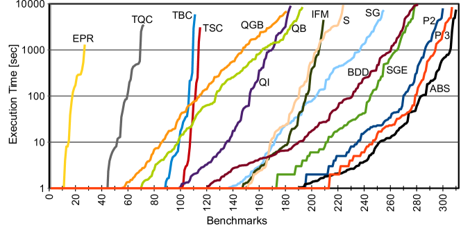
Figure 17: A cactus plot summarizing the execution times for computing a winning strategy with different methods and configurations.

Our reduction to EPR does not scale well. EPR could only solve $27$ instances. In none of the cases, a timeout was hit. For all instances that could not be solved, iProver ran out of memory.

Our template-based configurations solve only few instances. By comparing the lines for TQC and TBC, we can see that QBF preprocessing improves the scalability of our QBF-based realization of the template-based approach quite significantly. Our implementation TSC using CEGIS and SAT solving can even solve a few more instances. In all three cases, the lines rise very steeply. Slightly oversimplified, this means that the template-based methods either find a solution quickly or not at all. Unfortunately, the latter case happens more often. In total, TSC solves only 115 instances, which is low compared to the other methods. However, the solved instances include some that cannot be solved by any other method, so the template-based approach can complement other techniques. We will elaborate on this aspect in the next section. Except for the (very large) gb benchmarks, the memory limit was never exceeded.

Incremental QBF solving gives a solid speedup for simple benchmark instances. Compared to QB and QGB, the realization QI using incremental QBF solving is faster on average by more than one order of magnitude for simple benchmark instances. For example, the $130$ simplest instances for QB can all be solved by QB in less than $137$ seconds each, while the $130$ simplest instances for QI can be solved by QI in less than $6.2$ seconds each. Yet, for more complex instances, QI falls behind QB. One possible reason is the lack of QBF preprocessing in QI, which appears to be a promising future research direction.

SAT solvers can outperform QBF solvers when learning a winning region. All our QBF-based methods are outperformed significantly even by the plain SAT solver based implementation S. The observation that it can be beneficial to solve QBF problems with plain SAT solving is not new [74, 50], and hence not completely surprising. The plain implementation S can already solve more instances than our reimplementation IFM of the approach by Morgenstern et al. [74].

Optimization RG yields a speedup of roughly one order of magnitude for method S. This can be observed, at least for larger benchmark instances, when comparing the lines for SG and S in Figure 17. For example, the $224$ simplest instances for S can each be solved by S in at most $9450$ seconds. On the other hand, SG can solve its $224$ simplest instances in at most $470$ seconds, which is $20$ times shorter. Interestingly, optimization RG is not beneficial when applied to our QBF-based implementation (compare QGB versus QB) on the average over all our benchmarks, though. But even in the QBF case, it still yields a significant speedup for certain benchmark instances. While optimization RG turned out to be very effective, optimization RC does not have a positive effect on average in our experiments: the number of solved instances decreases from $255$ to $236$ when switching from SG to SGC (this is not shown in Figure 17 but can be seen in Table 3). But optimization RC is also beneficial for individual benchmark instances and, thus, not useless either.

Our heuristic for quantifier expansion gives a speedup of roughly one more order of magnitude. This can be seen by comparing the line for SGE with that for SG. Nailed down by numbers, SG solves its $254$ simplest benchmarks in at most $6800$ seconds each, while SGE solves its $254$ simplest benchmarks in at most $268$ seconds, which is $25$ times shorter. The configuration SGE is already on a par with BDD.

Our parallelization achieves a speedup of more than one additional order of magnitude. SGE solves its $279$ simplest benchmarks in at most $9920$ seconds each. P2 solves its $279$ simplest benchmarks in at most $295$ seconds, which is $33$ times shorter. P3 never requires more than $105$ seconds on its $279$ simplest benchmarks, which can even be seen as a speedup by a factor of $95$ over SGE. Obviously, these speedups are not primarily the result of exploiting hardware parallelism. They rather stem from combining different approaches that complement each other. Although AbsSynthe uses advanced techniques such as abstraction/refinement, P3 is not far behind (P3 solves $4$ instances less).

5.3.3 Performance per Benchmark Class

The previous section discussed the performance of the individual methods and configurations on average over all our benchmarks. In this section, we will perform a more fine-grained analysis for the different classes of benchmarks.

Table 3 lists the number of solved benchmark instances per benchmark class. The first line gives the total number of benchmarks in the class. The last column gives the total number of benchmarks for which a winning strategy could be computed by the respective method within $10\,000$ seconds and a memory limit of $8$ GB. Recall that a description of the compared methods and their configurations can be found in Table 2. Some statistics on the benchmarks can be found in Table 1. Table 3 marks the “best” configuration for a certain benchmark class in blue: If several methods solve the same amount of instances, we marked the one with the lowest total execution time. For cases where the difference in the total execution time is insignificant, we marked several configurations. If most of the configurations solve all instances of a certain benchmark class in an insignificant amount of time, we refrain from marking them. Moreover, we do not include ABS and the parallelizations in this ranking because they combine several techniques.

Table 3: Computing a winning strategy: solved instances per benchmark class.

	add	mult	cnt	mv	bs	stay	amba	genbuf	fact	mov	driver	demo	gb	load	ltl2dba	ltl2dpa	Total
Total	20	14	28	32	10	24	27	48	15	16	16	50	4	5	23	18	350
BDD	20	8	26	32	4	16	21	48	12	11	6	46	0	3	18	10	281
IFM	8	7	16	32	10	10	3	7	2	2	16	50	0	5	23	18	209
Q	8	4	24	30	10	10	2	7	1	0	2	44	0	2	20	15	179
QB	10	8	22	32	10	12	3	7	3	0	8	43	0	2	19	14	193
QGB	10	8	22	32	10	12	3	11	3	0	5	42	0	2	14	7	181
QGAB	10	8	22	32	10	12	3	11	3	0	4	42	0	1	6	9	173
QGCB	10	8	22	32	10	12	3	12	3	0	7	44	0	4	18	12	197
QI	8	4	22	30	10	10	3	7	2	0	2	45	0	3	22	16	184
S	8	7	24	32	10	18	15	13	2	2	3	46	0	4	23	17	224
SG	8	7	24	32	10	17	18	29	2	2	10	50	0	5	23	18	255
SGC	10	7	22	32	10	12	15	25	2	1	6	49	0	5	23	17	236
SE	20	9	24	32	10	12	19	20	3	2	3	48	0	4	23	18	247
SGE	20	9	24	32	10	12	21	37	5	3	10	50	0	5	23	18	279
TQC	10	9	24	12	4	10	0	0	0	0	0	3	0	0	0	0	72
TBC	20	14	24	25	6	18	0	0	0	0	0	4	0	0	0	0	111
TSC	8	7	28	32	10	24	0	0	0	0	0	6	0	0	0	0	115
EPR	4	2	11	8	0	2	0	0	0	0	0	0	0	0	0	0	27
P2	20	14	28	32	10	24	22	37	5	2	10	50	0	5	23	18	300
P3	20	14	28	32	10	24	23	37	5	2	16	50	0	5	23	18	307
ABS	20	9	24	32	10	16	27	48	11	11	7	50	0	5	23	18	311

add. Neither BDD nor the template-based method TBC require more than $0.2$ seconds for any instance of the add benchmark. The SAT solver based learning approaches using universal expansion (SE, SGE) solve all instances as well, but require up to $42$ seconds. Without expansion (S, SG, SGC), SatWin1 requires many iterations to refine $U$ before a counterexample is found or to conclude that no counterexample exists (see Algorithm 9). For instance, for add6y, roughly $4000$ counterexample candidates are computed. This takes only one second. For add8y, SatWin1 already computes $65\,000$ counterexample candidates, which takes $90$ seconds. For add10y we hit the timeout. In contrast, the QBF-based learning methods (with names starting with Q) require only two iterations, but cannot solve significantly more instances either. This illustrates that the number of iterations alone is often not a good measure for estimating the performance of different algorithms relative to each other.

mult. The results for this benchmark are similar to add. The main difference is that the BDD-based implementation does not perform well, but this is not surprising since multipliers are known to be challenging for BDDs (see Section 2.2.1). Even ABS, which is highly optimized but also BDD-based, cannot solve all mult instances. The template-based configuration TBC performs best.

cnt. When the winning region is computed iteratively for this benchmark, this requires many iterations. More specifically, around $2^{k-1}$ refinements of the winning region are required for cnt$ko$. For $k=30$, this already gives around half a billion iterations. Even though the time per iteration is very low for all configurations, this still results in timeouts for large values of $k$. In contrast, the template-based realizations require only one iteration. In particular, the configuration TSC solves all cnt instances in less than $8$ seconds.

mv. Even though this benchmark has a relatively high number of inputs and control signals, most methods can solve all its instances within a fraction of a second. This benchmark will only be challenging for some of our circuit computation methods in Section 5.4.

bs. This benchmark contains a barrel shifter and is thus challenging for BDD. Most of the other methods solve all instances within a fraction of a second.

stay. This benchmark contains a counter and a multiplier, and thus combines the characteristics of mult and cnt. Hence, it is not surprising that one of the template-based configurations performs best.

amba and genbuf. While the previous benchmarks are basically toy examples designed to challenge the synthesis methods in different ways, the amba and genbuf benchmarks specify realistic hardware designs. BDD performs very well on both these benchmarks. One circumstance contributing to this success may be that these benchmarks have been translated from input files for the BDD-based synthesis tool Ratsy [83], where they have been tweaked for efficient synthesizability. Yet, the SAT-based learning method SGE solves the same amount of amba instances as BDD, an is even slightly faster on the solved instances. For genbuf, BDD is unrivaled in our experiments.

fact and mov. None of our SAT-based methods can compete with BDDs on these benchmarks.

driver. The IFM method by Morgenstern et al. [74] solves all instances of the driver benchmark in a fraction of a second. This is remarkable because with up to $326$ state variables, these benchmarks are quite large. The SAT solver based learning methods SG and SGE are ranked second when run with optimization RG. Without optimization RG, only few instances can be solved.

demo. Both IFM and SGE can solve all instances in at most $40$ seconds. With up to $280$ state variables, the demo benchmarks contain quite large instances as well. The number of inputs is always relatively low, though.

gb. These benchmarks are far beyond reach with any of our methods. Even ABS fails.

load, ltl2dba and ltl2dpa. SGE performs best, solving most of these instances in less than a second. With $138$ seconds, the longest execution time with SGE is also quite low.

Conclusions. Our QBF-based learning algorithms are dominated by our SAT solver based realizations across all benchmarks classes. EPR is even dominated by all other configurations. On the other hand, no single methods dominates all the other methods on all benchmark classes. We thus conclude that it is important to have different synthesis approaches available. Our experiments suggest that our novel SAT-based synthesis methods form an important contribution to the portfolio of available methods, complementing existing BDD-based methods (like BDD and ABS) but also existing SAT-based methods (like IFM).

5.3.4 Further Observations

This section highlights interesting observations that are more specific to certain methods.

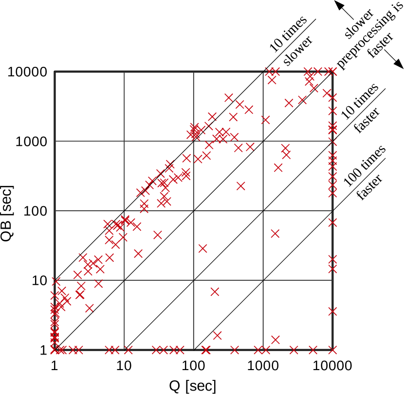
Figure 18: A scatter plot illustrating the speedup due to QBF preprocessing in QBF-based learning (Q versus QB).

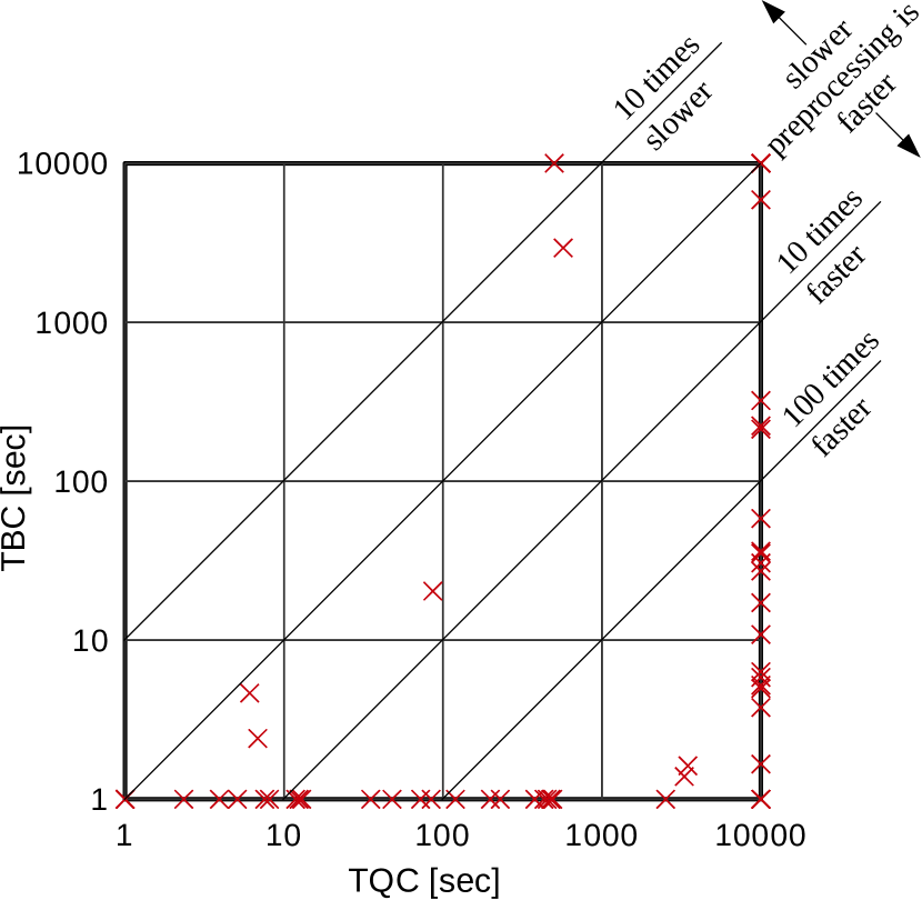
Figure 19: A scatter plot illustrating the speedup due to QBF preprocessing in our template-based approach (TQC versus TBC).

QBF preprocessing is important. Figure 19 compares the execution times with and without QBF preprocessing for the QBF-based learning approach in a scatter plot. Each point in the diagram corresponds to one benchmark instance. The horizontal axis gives the execution time for the benchmark without preprocessing, and the vertical axis the corresponding execution time with preprocessing. Hence, all points below the diagonal represent a speedup due to preprocessing, and all points above are instances with a slowdown. Note that both axes are scaled logarithmically. We can see a slowdown by up to around one order of magnitude for many instances. However, there are also $20$ points on the x-axis, indicating instances that can be solved in less than one second due to preprocessing. Furthermore, there are $19$ points on the right border of the diagram, indicating cases where we had a timeout without preprocessing but get a solution when preprocessing is enabled. Two instances are even located in the lower right corner, representing an improvement from a timeout to less than one second. The number of solved instances increases from $179$ to $193$ due to preprocessing in the QBF-based learning method (see Table 3). The results for the template-based method (TQC versus TBC) are illustrated in Figure 19 and are even more impressive. A noticeable slowdown can only be observed for two cases. There are $44$ points on the x-axis, for which preprocessing reduced the execution time to less than one second. For $40$ cases, a timeout is avoided due to preprocessing. Finally, there are $23$ points in the bottom right corner of Figure 19, for which a timeout is turned into a successful execution that takes less than one second.

Our optimizations for quantifier expansion can avoid a formula size explosion in many cases. For most of our SAT-based methods, the memory consumption is rather insignificant. As an exception, SGE can consume quite some memory due the expansion of universal quantifiers (see Section 3.3). However, our implementation can also fall back to SG if some memory limit is exceeded. In our experiments, this happened only for large instances of mult, stay, gb, and driver. One reason is our careful implementation of the expansion, which aggressively applies simplifications to reduce the formula blow-up. As an example, for genbuf15b, a straightforward implementation would produce $652\cdot 2^{23}\approx 5\cdot 10^{9}$ AND gates to define the expanded transition relation. With $3\cdot 4=12$ byte per AND gate, this gives $56$ GB. With our simplification techniques, the expanded transition relation has “only” $1.5$ million AND gates. In addition, the final over-approximation $F$ of the winning region $W$ for genbuf15b contains $707$ clauses and $8517$ literals (after simplification). After negation, this makes $8517$ clauses with $17739$ literals. With $4$ byte per literal, combining $2^{23}$ copies of this CNF in a straightforward way would require more than $500$ GB of memory. Due to our simplifications, the expanded CNF for $\neg F$ has only $8.5$ million literals and SGE solves this benchmark instance without falling back to SG. The maximum memory consumption is only $680$ MB.

Our parallelization is more than a portfolio approach. When executed with two threads, our parallelization combines the template-based approach (in a mix of TBC and TSC) with the learning-based approach SGE. The two approaches do not only run in isolation, but share information: clauses discovered by the SGE-thread are communicated to the template-based thread and are considered as fixed part of the winning region there (see Section 3.7). This exchange of information can have a positive effect. For example, for the genbuf benchmark, the template-based approach fails to solve even the simplest instances when applied in isolation. However, in our parallelization, the final winning region for certain instances is actually found by the template-based thread. This includes even very large instances such as genbuf15b. The speedup of our parallelization P2 in comparison to SGE for such instances is rather moderate (e.g. $\approx 10\,\%$ for genbuf15b), but this still illustrates that complementary methods can benefit from each other in our parallelization.

5.4 Circuit Synthesis Results

We now compare our different methods (from Chapter 4) to construct a circuit from a given strategy. Again, we first describe the evaluated configurations and the experimental setup. Section 5.4.3 then discusses the results on the average over all our benchmarks. Section 5.4.4 dives into more details by investigating the performance for different benchmark classes. Other interesting observations will be highlighted in Section 5.4.5.

5.4.1 Evaluated Configurations

Table 4 lists the different methods and their configurations compared in this section. All our SAT-based methods use the tool ABC [67] in a postprocessing step to further reduce the circuit size.

Baseline. BDD denotes a BDD-based implementation of the standard cofactor-based approach presented in Algorithm 2. It is implemented in the tool that has already been discussed in Section 5.3.1, which won a synthesis competition that has been carried out in the course of a lecture. Besides dynamic variable reordering (with method SIFT [40, 41]), it also performs a forced reordering with a more expensive heuristic (SIFT_CONV [40, 41]) before circuits are extracted from the strategy. Furthermore, it uses a cache that maps BDD nodes to corresponding signals in the circuit constructed so far. Whenever new circuitry is added, the cache is consulted to reuse existing signals. Consequently, no two signals in the constructed circuit will be equivalent. The configuration ABS denotes the circuit synthesis step as implemented in AbsSynthe version 2.0 [13]. The basic algorithm is the same as that of BDD, but additional optimizations are applied. The IFM method by Morgenstern et al. [74], which has been used as a baseline in Section 5.3, is not included here because it can only compute a winning strategy but not a circuit implementing it.

QBF-based methods. Our approach using QBF certification (see Section 4.1) is named QC. A variant where we compute the negation of the winning region using the procedure NegLearn (Algorithm 11) is denoted by QCN. Our QBF-based learning approach from Algorithm 13 is used in three configurations: QL denotes a plain implementation using DepQBF, QLB also uses QBF preprocessing by Bloqqer, and QLI uses the DepQBF solver in an incremental fashion (see Section 4.2.2).

Interpolation-based method. An implementation of the interpolation-based method from Algorithm 15 is denoted by ID. It applies the dependency optimization presented in Section 4.3.2 and uses MathSAT version 5.2.12 as interpolation engine. MathSAT supports several interpolation methods. In our experiments we use McMillan’s system [84]. Results with other interpolation methods are rather similar, though. We also implemented our own interpolation engine by processing PicoSAT proofs in the TraceCheck format. However, for larger benchmark instances, the proof files grew prohibitively large with this approach. Our realization using MathSAT does not have this problem.

Learning based on SAT solvers. Configuration SL implements the SAT solver based learning approach from Section 4.4 without the dependency optimization (Section 4.3.2) and without minimizing the final solution (Section 4.4.2). SLD denotes a similar configuration, but with the dependency optimization enabled. Finally, the SLDM configuration also applies a minimization of the final solution by attempting to eliminate literals and clauses from the computed solutions (Section 4.4.2). All these configurations use activation variables to perform incremental solving across all calls to CnfInterpol (see Section 4.4.2). Lingeling is slightly faster on average than MiniSat and PicoSAT in all these configuration. Results for other configurations ($28$ in total) can be found in the downloadable archive.

Table 4: Configurations for computing a circuit that implements a given strategy.

Name	Algorithm and Optimizations	Solver
BDD	CofSynt (Alg. 2)	CuDD
ABS	AbsSynthe 2.0 [13]	CuDD
QC	QBF Certification (Sect. 4.1)	QBFCert
QCN	QBF Certification (Sect. 4.1) + NegLearn (Alg. 11)	QBFCert
QL	SafeQbfSynt (Alg. 13)	DepQBF
QLB	SafeQbfSynt (Alg. 13)	DepQBF + Bloqqer
QLI	SafeQbfSynt (Alg. 13)	Incremental DepQBF
ID	SafeInterpolSynt (Alg. 15) + Dep. Opt. (Sect. 4.3.2)	MathSAT
SL	SafeInterpolSynt + CnfInterpol (Alg. 16)	Lingeling
SLD	SafeInterpolSynt + CnfInterpol (Alg. 16) + Dep. Opt. (Sect. 4.3.2)	Lingeling
SLDM	SafeInterpolSynt + CnfInterpol (Alg. 16)	Lingeling
	+ Dep. Opt. + Minimizing the final solution (Sect. 4.4.2)
P2	Parallel (Sect. 4.5) with 2 threads	Lingeling + DepQBF
P3	Parallel (Sect. 4.5) with 3 threads	Lingeling + DepQBF

5.4.2 Experimental Setup

Again, all experiments were performed on an Intel Xeon E5430 CPU with 4 cores running at $2.66$ GHz, using a 64 bit Linux as operating system. A timeout was set to $10\,000$ seconds for all circuit synthesis runs. The available main memory was limited to $8$ GB. The maximum size for auxiliary files to be written to the hard disk was set to $20$ GB.

Sanity checks. All synthesized circuits were model checked using IC3 [24]. IC3 never found a counterexample but in some cases hit a timeout. We thus also ran a bounded model checker (BLIMC, which is distributed with Lingeling [78]) to get bounded correctness guarantees for such cases.

Winning strategies. For all our SAT-based circuit computation methods, we used the winning strategies as computed by configuration P3 (see Table 2). Preliminary experiments with other strategy computation methods suggest that the impact on the performance in circuit synthesis is rather small. One reason is that we simplify the computed winning region (or winning area) by calling CompressCnf (Algorithm 7) as a preprocessing step to circuit extraction (see Chapter 4). We thus refrain from running experiments with all combinations of our strategy- and circuit computation methods. Furthermore, we stored the winning strategies computed by P3 into files and loaded them for our circuit computation experiments in order to ensure that all our methods operate on exactly the same strategy (and to save computational resources for recomputing the strategy each time). For BDD and ABS, we used the winning regions as computed by these tools as a starting point for circuit synthesis.

Benchmarks. From the $350$ benchmark instances used to evaluate our strategy computation methods (see Section 5.2), only $267$ instances have been used to compare our circuit computation methods. This has two reasons. First, $40$ instances are unrealizable, so they have no winning strategy. Second, for some instances, no winning strategy could be computed (even with a timeout of $10^{5}$ seconds) for at least one of the compared methods. In order to have a fair comparison, we thus used only those benchmarks for which P3, BDD and ABS succeeded in computing a winning strategy. In detail, P3 failed to compute a winning strategy for $25$ instances. For $19$ additional instances, BDD could not find a winning strategy within $10^{5}$ seconds. This includes cnt$30$n and cnt$30$y, for which we estimated BDD’s circuit synthesis time (to be $0.1$ seconds) and the circuit size (to be $32$ gates) based on observations from smaller instances. This leaves $17$ excluded instances. ABS could not compute a winning strategy for $11$ more benchmarks. However, for two cnt instances, we could estimate the time and size to $0.1$ seconds and $1$ gate based on results for smaller instances. For eight instances of the stay$ko$ benchmark, we also estimated $0.1$ seconds and $k+1$ gates. What remains is one driver instance to exclude. This results in $350-40-25-17-1=267$ instances used for the comparison. The number of used instances per benchmark class can be seen from Table 5 (see the line labeled “Total”).

More detailed comparisons. The downloadable archive also contains more detailed pairwise comparisons on larger subsets of the benchmark instances. This includes charts to compare our SAT-based methods with ABS on all $281$ benchmarks for which both ABS and P3 were able to compute a winning strategy. Charts comparing our SAT-based methods with BDD on all $268$ instance on which both BDD and P3 were able could find a winning region are included as well. However, since the results are almost identical to our three-way comparison, we refrain from presenting them in this article.

5.4.3 The Big Picture

The Figures 21 and 21 contain cactus plots illustrating the execution time and the resulting circuit size for the method configurations from Table 4. Configuration QC is omitted because both the execution time and the circuit size is similar to QCN (the difference is mostly in the memory consumption). Configuration QL performs slightly worse than QLB and QLI and is also omitted to make the plots more legible. The following paragraphs discuss the most important observations based on these two figures. A detailed analysis is done in Section 5.4.4 and 5.4.5.

Figure 20: A cactus plot summarizing execution times for computing a circuit from a strategy.

Figure 21: A cactus plot summarizing the resulting circuit sizes.

QBF certification does not perform well. From Figure 21, we can see that the QBF certification method QCN produces the largest circuits. Figure 21 illustrates that QCN is on average slightly faster than QLB, but still solves less instances within the given resource limits. The reason is that QCN often exceeds the $20$ GB limit for auxiliary files because the proof traces produced by DepQBF in the QBFCert framework can grow very large (several hundreds of GB when run without limits).

QBF-based learning is slow but produces small circuits. Especially when used with incremental QBF solving, QBF-based learning can outperform QBF certification both regarding execution time and circuit size (compare QLI versus QCN). Still, in comparison with the other methods, QLI is on average way slower. Regarding circuit size, QLI and QLB are on a par and outperform the interpolation-based method ID as well as the BDD-based implementation BDD by almost one order of magnitude on average.

The interpolation-based approach does not outperform BDDs in our experiments. Regarding circuit size, the interpolation-based configuration ID yields similar results as BDD on average. However, ID is noticeably slower than BDD, especially for more complex benchmark instances.

Our SAT solver based learning approach outperforms all our other non-parallel methods. This holds true for both the execution time and the circuit size. Configuration SLD turns out to be our best non-parallel option on the average over all our benchmarks. It is already faster than BDD on average by more than one order of magnitude. For example, BDD can solve its $233$ simplest benchmark instances in at most $7931$ seconds each. SLD never needs more than $461$ seconds for its $233$ simplest instances. This is a factor of $17$. With respect to circuit size, the situation is even more extreme. The $233$ smallest circuits produced by BDD have at most half a million AND gates each. The $233$ smallest circuits produced by SLD have at most $2383$ gates each. This is smaller by a factor of $188$. SLDM produces even slightly smaller circuits, with an improvement factor of $240$ compared to BDD. This is not only because BDD produces large circuits for benchmarks that cannot be solved by SLD. The most extreme instance is driverd8, for which BDD produces a circuit with $3.7$ million AND gates, while SLD produces a circuit with only $66$ gates.

Our parallelization is competitive with the state of the art. Our parallelization P3 increases the number of solved instances compared to SLD from $250$ to $263$ by combining different methods and optimizations. The circuit sizes also decrease slightly, which is partly due to our heuristics performing additional circuit minimizations if there is sufficient time left (see Section 4.5), and due to selecting the smallest solution from all threads. Our parallelization already solves $2$ instances more than the state-of-the-art tool AbsSynthe. When comparing P3 against AbsSynthe in Figure 21, we can see that AbsSynthe solves many instances in less than one second but the execution times grow steeper for more difficult instances. Thus, AbsSynthe can be superior if the timeout is short, while P3 shows a more steady pace. Regarding circuit size, our parallelization outperforms AbsSynthe by more than one order of magnitude on average (compare P3 versus ABS in Figure 21).

Execution time and circuit size often correlate. With the exception of the QBF-based learning methods, we can observe a correlation between execution time and circuit size in our experiments. Methods that are fast have a tendency to also producing small circuits and vice versa. At the first glance, this may be surprising because, intuitively, one could expect that we have to find a good trade-off between these performance metrics. One reason for the correlation is that most of our methods (all except QC and QCN) compute circuits iteratively for one control signal after the other. After every iteration, the strategy formula is refined with the solutions for the control signals that have been synthesized so far. If these solutions are complicated, then this results in more complicated strategy formulas for the next iterations, which can increase the computation times. For the learning-based methods, the size of the CNF formulas defining the control signals directly corresponds to the number of iterations that were needed to compute them: Every clause results from a mayor iteration involving a counterexample computation. Every literal in a clause witnesses a failed attempt to eliminate this literal with a SAT- or QBF solver call. A correlation between the circuit size and the execution time is thus natural.

Computing circuits from strategies is by no means a negligible step in the synthesis process. Let us compare the total strategy computation time against the total circuit computation time for all instances where both steps terminate within the timeout of $10\,000$ seconds. For P3, this comparison reveals that $52$ percent of the total synthesis time is spent on strategy computation and $48$ percent is consumed by circuit computation. For BDD, the distribution is $60\,\%$ to $40\,\%$. Only for ABS, the distribution is $90\,\%$ to $10\,\%$, which may be due to the abstraction/refinement techniques implemented in ABS.

5.4.4 Performance per Benchmark Class

This section analyzes the performance of our methods for circuit synthesis for the different benchmark classes. We will see that the configuration SLD is not always superior.

Table 5 lists the number of benchmark instances that could be solved per benchmark class by the different configurations. The first line gives the total number of benchmark instances in the respective class. The last column gives the total number of instances for which a circuit could be computed by the respective method within the given resource limits ($10\,000$ seconds, $8$ GB of main memory, $20$ GB for auxiliary files). The fastest configuration is marked in blue. If the same amount of instances are solved by several configurations, we marked the one with the lowest total execution time. In case the total execution time is very similar, we sometimes marked several configurations. For benchmark classes where most of the configurations solve all instances, we did not mark any configuration. Again, we do not include ABS and the parallelizations in this ranking because they combine several techniques.

Table 5: Computing a circuit from a strategy: solved instances per benchmark class.

	add	mult	cnt	mv	bs	stay	amba	genbuf	fact	mov	driver	demo	load	ltl2dba	ltl2dpa	Total
Total	20	14	28	32	10	24	23	42	3	2	0	37	3	19	10	267
BDD	20	7	28	32	4	16	13	41	3	2	-	36	3	18	10	233
QC	6	4	28	32	10	24	0	6	2	0	-	30	2	7	10	161
QCN	6	4	28	32	10	24	3	10	3	1	-	31	2	9	8	171
QL	8	4	28	32	10	24	3	10	2	0	-	35	3	19	10	188
QLB	8	3	28	32	10	24	3	9	2	0	-	35	3	19	10	186
QLI	8	4	28	32	10	24	3	11	3	1	-	35	3	19	10	191
ID	20	5	28	28	10	24	4	12	2	1	-	36	3	19	10	202
SL	12	5	28	25	10	24	20	41	3	2	-	37	3	19	10	239
SLD	20	14	28	22	10	24	17	41	3	2	-	37	3	19	10	250
SLDM	20	14	28	22	10	24	14	40	3	1	-	37	3	19	10	245
P2	20	14	28	32	10	24	17	41	3	2	-	37	3	19	10	260
P3	20	14	28	32	10	24	20	41	3	2	-	37	3	19	10	263
ABS	20	8	28	32	10	24	23	42	3	2	-	37	3	19	10	261

add. The configurations BDD, SLD and SLDM solve all instances of the add benchmark within one second. The difference in circuit size is moderate (at most $171$ gates with SLD and SLDM; at most $416$ gates with BDD). The interpolation-based method ID solves all instances as well but requires at most $40$ seconds. The good results of SLD, SLDM and ID are mostly due to our dependency optimization (see Section 4.3.2 and Section 4.4.2): Without the dependency optimization, the SAT solver based learning method solves only $12$ instances (SLD versus SL).

mult. This benchmark is similar to add in spirit, but the circuit to be synthesized is more complex. SLD and SLDM still perform well, again due to the dependency optimization. However, BDD and ID fall back noticeably. The difference in circuit size also grows more significant: For example, BDD implements mult9 with more than $10^{5}$ gates, while SLD and SLDM require only $633$ gates. One reason is that multipliers cannot be represented by small (monolithic) BDDs with any variable ordering (see Section 2.2.1). Since the BDD method dumps BDDs as a network of multiplexers to obtain the resulting circuit, the BDD size does not only affect the computation time but also the resulting circuit size. Our SAT solving based methods SLD and SLDM do not suffer from this issue. They even outperform AbsSynthe significantly on this benchmark.

cnt, bs  and stay. These benchmarks can be solved by all our methods in a few seconds. Only ID requires up to $46$ seconds on larger instances of stay. BDD performs well on cnt, but cannot solve all instances of bs and stay. The latter two benchmarks contain barrel shifters and multipliers, which are known to be challenging for BDDs.

mv. The mv benchmark is an interesting case. Most of our methods can solve all instances of this benchmark in less than one second. However, for the interpolation-based method ID as well as the SAT solver based learning methods SL, SLD and SLDM, this benchmark is challenging. All these methods are based on InterpolSynt (Algorithm 14). The crux with the mv benchmark is that the XOR sum of all control signals must be $\mathsf{true}$. InterpolSynt starts by building a circuit to fix the value of the last control signal based on all other control signals such that this is ensured. Since this circuit needs to react properly to all possible values of all other control signals, it can be very large. In particular, the SAT solver based learning methods build this circuit in a CNF representation without introducing auxiliary variables. A CNF formula that computes the XOR sum of $n$ variables without introducing new auxiliary variables requires $2^{n-1}$ clauses. For mv28y, this gives $2^{27}\approx 134\cdot 10^{6}$ clauses. Only in the last iteration, when the algorithm processes the first control signal, InterpolSynt discovers that this signal can actually be set to a constant value. This has the effect that all the computed circuits for the other control signals also collapse to constant values. The root cause for this behavior is that InterpolSynt is very conservative with exploiting implementation freedom (see Section 4.3.4 for a discussion). In contrast, the QBF-based learning algorithm QbfSynt (Algorithm 12) exploits the available freedom greedily. It sets each control signal to a constant value right away, because this is sufficient to ensure that a solution for the remaining control signals still exists.

amba and genbuf. For these benchmarks, the SAT solver based learning configuration SL performs best. That is, the dependency optimization implemented in SLD and SLDM does not pay off. SLD, SL and BDD can solve the same amount of genbuf instances, but SLD is slower than SL by a factor of $2$ in total, and BDD is even slightly slower than SLD in total. The sum of the circuit sizes for all genbuf instances is $44$ times smaller when using SL instead of BDD. For amba, the factor is $21$ when counting only the instances that can be solved by both SL and BDD.

fact and mov. Both BDD and SL can solve all fact instances in less than $10$ seconds per instance. The mov instances are solved by BDD in at most $160$ seconds per instance. The second fastest configuration for mov is SL, but it requires already $4500$ seconds.

driver. ABS cannot compute a winning strategy for any of the driver instances, so this benchmark is not included in the comparison of Table 5. Our SAT solver based learning methods SL, SLD and SLDM can solve all driver instances in less than $10$ seconds. The circuit size with these methods is at most $600$ gates. BDD can only handle the smallest driver instance, but takes already half an hour to produce a circuit with $3.7$ million gates. With up to $326$ state variables and $98$ inputs, the driver benchmark certainly offers plenty of possibilities for building complicated circuitry. Yet, in contrast to BDD, our learning-based methods appear to perform well in exploiting the implementation freedom to avoid overly complicated solutions.

demo. Only ABS and our SAT solver based learning methods SL, SLD and SLDM can solve all instances. The dependency optimization is not beneficial: SLD is slower than SL by a factor of $3.2$.

load. Again, the SAT solver based learning methods SL, SLD and SLDM perform best: they solve all instances in at most $2$ seconds. ID requires up to $18$ seconds. The fastest QBF-based learning method is QLI, requiring up to $87$ seconds for the load instances. BDD requires up to $10$ minutes.

ltl2dba and ltl2dpa. The configurations ID, SL, SLD, and SLDM require at most $4$ seconds on these benchmarks. Other configurations that can also solve all these benchmarks are slightly slower.

5.4.5 Further Observations

The effect of our postprocessing with ABC [67] is rather insignificant. For SLD, ABC manages to reduce the average circuit size from $9500$ gates to around $2700$ gates in our experiments. However, this average is strongly influenced by the mv benchmark, where circuits with up to half a million gates are reduced to circuits were all control signals are driven by constants. See Section 5.4.4 for an explanation why this happens. This reduction for the mv benchmark could also be achieved with a simple constant propagation. When omitting the mv benchmark, the average circuit size is reduced from $4100$ gates to $2900$ gates, which is a reduction by around $30$ percent. In relation to the circuit size differences between our methods, which can be in the range of several orders of magnitude (see Figure 21), this is rather insignificant. On the other hand, in the case of SLD, only $0.6$ percent of the total execution time for all benchmarks is spent by ABC. By modifying the sequence of minimization commands executed by ABC, other trade-offs between the execution time and the resulting circuit size improvements are possible. Yet, our experiments suggest that postprocessing cannot easily compensate the large circuit size differences between the methods. In other words, exploiting the implementation freedom cleverly while computing the circuits appears to be much more effective than investing more effort into postprocessing.

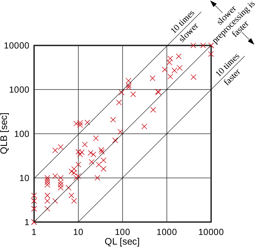
Figure 22: The effect of QBF preprocessing in circuit synthesis.

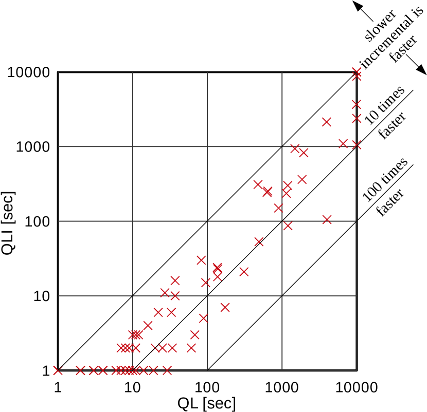
Figure 23: The effect of incremental QBF solving in circuit synthesis.

Incremental QBF solving outperforms QBF preprocessing in our circuit synthesis experiments. Figure 23 illustrates the effect of QBF preprocessing in our QBF-based learning method for circuit synthesis by comparing QLB against QL in a scatter plot. We see a negative effect for most instances. The number of solved instances even decreases from $188$ to $186$ (see Table 5). By trend, preprocessing is more beneficial for more complex instances. Some of the more complex instances have been left out in the comparison because either BDD or ABS failed to compute a winning region. If we consider all $285$ instances on which P3 managed to compute a winning strategy, the number of solved instances actually increases from $190$ to $193$ due to QBF preprocessing. Hence, preprocessing also has its merits. On the other hand, incremental QBF solving has an exclusively positive impact in our experiments. It is visualized in Figure 23, comparing QLI against QL. There is not a single instance where incremental QBF solving increased the computation time. In $3$ cases, a timeout is avoided. When counting only the instances where QL terminates successfully, the average execution time is reduced from $204$ to $59$ seconds, which is a speedup of factor $3.5$.

Using NegLearn reduces the memory required by QBFCert. As already mentioned, QBFCert can consume quite some memory. This applies to both main memory as well as disk space for auxiliary files. As a consequence, QC encounters a timeout for only two benchmark instances. For the other instances that cannot be solved, the reason is in exceeding the memory limit. When using NegLearn (Algorithm 11) in order to compute the negation of the winning region without introducing auxiliary variables, the size of the auxiliary files is reduced by up to a factor of $30$. On the other hand, for more than $15$ instances, running NegLearn only trades a memory issue for a timeout. Still, the total number of solved instances increases from $161$ to $171$ in our QBF certification approach (compare QC with QCN in Table 5). For our other methods, running NegLearn does not pay off, though.

Minimizing the final solution in SAT solver based learning yields moderate circuit reductions. When counting only the benchmark instances where both SLD and SLDM terminate, the average circuit size is reduced by $33\%$ (from $1500$ to $1000$ gates) due to the final minimization step discussed in Section 4.4.2. On the other hand, the average circuit computation time increases from $106$ seconds to $311$ seconds, which is almost a factor of $3$. For individual benchmark instances, the cost/benefit ratio can be lower, though. For example, in the case of driverb8, the circuit size is reduced from $594$ gates to $152$ gates in only a few extra seconds.

5.5 Discussion

Binary Decision Diagrams are increasingly displaced by SAT-based methods in the formal verification of hardware circuits. In synthesis, however, outperforming BDDs is challenging.

Outperforming BDDs in strategy computation. For the strategy computation step, our SAT solver based learning approach is competitive with the BDD-based reference implementation in our experiments, but only when making clever use of incremental solving, unsatisfiable cores, our optimization for exploiting unreachable states, and our heuristic for expanding quantifiers. With our parallelization, we can even solve significantly more benchmark instances than the BDD-based implementation. This is achieved by complementing the SAT solver based learning approach with our template-based approach. An advantage of BDDs is that they can handle both universal and existential quantification. This also holds true for QBF solvers. However, a QBF solver only computes one satisfying assignment, while BDDs eliminate the quantifiers to represent all satisfying assignments simultaneously. Our QBF-based algorithms have to compensate for that with more iterations. The performance of our QBF-based algorithms is rather limited compared to our SAT solver based realizations. This is somewhat surprising because the lack of universal quantification induces even more iterations. However, considering that QBF is still a rather young research discipline, this situation may change in the future. A combination of incremental QBF solving with preprocessing appears to be a particularly promising direction. Our parallelization is on a par with the state-of-the-art synthesis tool AbsSynthe, which is also BDD-based but uses abstraction/refinement and other advanced optimizations. Adopting optimizations like abstraction/refinement from AbsSynthe appears to be a promising direction for future work.

Outperforming BDDs in circuit computation. For the second synthesis step, where circuits implementing the computed strategies are constructed, our satisfiability-based methods are even more beneficial on average over all our benchmarks. In particular, our combination of interpolation with SAT solver based learning outperforms the BDD-based reference implementation by roughly one order of magnitude on average. Moreover, it produces circuits that are smaller by around two orders of magnitude. One reason is that the learning techniques we apply seem to be good at exploiting implementation freedom. Ehlers et al. [61] showed that learning techniques can also improve the circuit sizes when used with BDDs, but only at the cost of additional computation time. The experiments in this article suggest that the combination of learning algorithms with decision procedures for satisfiability is more promising. Our plain SAT solver based learning approach is still significantly slower than AbsSynthe. However, our parallelization can already solve more instances by combining different SAT-based methods. Moreover, it produces circuits that are smaller than those from AbsSynthe by more than one order of magnitude on average in our experiments.

Conclusion. BDDs are far from obsolete in the synthesis of reactive systems. Yet, SAT-based methods can be competitive, and even outperform BDD-based implementations on average when designed carefully. We also observed that SAT-based methods can solve classes of benchmarks that are hard to deal with for BDDs. We therefore believe that our novel synthesis methods form an important contribution to the portfolio of available approaches.

6 Related Work

Related work on which this thesis builds has already been discussed throughout the document, and especially in Chapter 2. This chapter discusses alternative approaches and points out similarities and differences.

6.1 SAT-Based Reactive Synthesis Approaches

Reactive synthesis is a broad research area, but approaches based on decision procedures for satisfiability are rare.

Incremental induction. Morgenstern et al. [74] present a SAT solver based synthesis algorithm for safety specifications that is inspired by the model checking algorithm IC3 [24] and its principle of incremental induction. The basic idea is to lazily compute the rank of the initial state of the specification, which is the maximum number of steps in which the environment can enforce to visit an unsafe state. If this rank is found to be finite, the specification is unrealizable. If it is found to be infinite, the specification is realizable. Hence, strictly speaking, the paper only presents a decision procedure for realizability. However, computing a winning strategy and a circuit implementing this strategy is also possible. We used a reimplementation of this algorithm as a baseline in our experimental evaluation. It was very fast on certain benchmark instances, but outperformed significantly by our new algorithms on average.

Property-directed synthesis. Chiang and Jiang [85] present a similar approach, which is also inspired by IC3 [24]. While Morgenstern et al. [74] solve the game from the perspective of the environment taking the unsafe states as anchor, the approach by Chiang and Jiang [85] takes the perspective of the controller to be synthesized. It uses the initial states as anchor and tries to avoid ending up in an unsafe state. This yields promising results for a (rather small) subset of the SyntComp 2014 benchmarks. An integration into our parallelization would be interesting.

Strategy computation without preimages. Narodytska et al. [86] propose an algorithm to compute strategies for reachability specifications, where a set of target states needs to be visited at least once. The general idea is to apply a counterexample-guided backtracking search in order to find a set of executions that is sufficient to reach the target states within some number $n$ of steps. This set of executions is then generalized into a winning strategy in the form of a tree that defines control actions based on previous inputs. If no strategy is found for a particular bound $n$, then $n$ is increased. A SAT solver is used both to compute and to generalize executions. Hence, in comparison to our work, this approach operates on a different specification class (reachability rather than safety), and it computes a winning strategy directly rather than deriving it from a winning region.

Implementing strategy trees. Eén et al. [87] complete the work discussed in the previous paragraph by proposing a method to compute circuits implementing the obtained winning strategies. Just like one of our methods, it uses interpolation. However, since the strategies are represented as trees rather than relations, the use of interpolation is quite different compared to our work.

QBF-based approaches. Staber and Bloem [65] present a QBF-based synthesis method for safety specifications. The general principle of unrolling the transition relation has already been discussed along with its drawbacks in Section 3.1.1 as a motivation for our learning-based algorithms. A solution for Büchi objectives (where some set of states needs to be visited infinitely often) is presented by Staber and Bloem [65] as well. Alur et al. [88] propose a similar solution for bounded reachability specifications (where a set of target states needs to be reached within at most $n$ steps). That paper [88] also proposes an optimization that uses only one copy of the transition relation. However, all variables are still copied for all time steps and the high number of quantifier alternations (linear in $n$) remains. In contrast, our learning-based methods use only one copy of the transition relation and two quantifier alternations in all QBF solver calls (at the cost of a potentially higher number of solver calls).

ALLQBF solving. Becker et al. [89] explain how QBF solvers can be used to compute not only one but all satisfying assignments of a QBF in the form of a compact (quantifier-free) formula. Similar to some of our satisfiability-based synthesis methods, query learning is used to solve this problem. The paper also points out that such an ALLQBF engine can be used as a direct replacement of BDDs to compute the winning region of various specification classes using fixpoint algorithms. For instance, Algorithm 1 can be realized with an ALLQBF engine in order to compute the winning region of a safety specification. While our QBF-based algorithm QbfWin (Algorithm 6) is similar in spirit, there are also some important differences. We apply query learning directly to the specification rather than the preimage computations, which allows for better generalizations. Furthermore, we extend the basic algorithm with additional optimizations such as our reachability optimization from Section 3.4.

QBF as a game. Synthesis can be seen as a game between two players: the system controlling the outputs and trying to satisfy the specification, and the environment controlling the inputs and trying to violate the specification. Similarly, QBF solving can also be seen as a game between two players: one player controls the existentially quantified variables and tries to satisfy the formula, the other player controls the universal variables and tries to falsify the formula. This idea is followed by Janota et al. [50] in the QBF solver RAReQS. Following the principle of counterexample-guided refinement of solution candidates, it uses two competing SAT solvers to build a QBF solver: one SAT solver computes candidates in the form of assignments to existential variables, the other one refutes them with assignments for the universal variables. We followed the same principle when traversing from our QBF-based synthesis algorithm to SAT solver based algorithms (cp. Algorithm 6 with Algorithm 9). However, we apply the idea on the level of the synthesis algorithm rather than for realizing individual QBF solver calls. This allows for additional optimizations. Another connection to this work is in coming to the same conclusion, namely that solving quantified problems with SAT solvers instead of QBF solvers can be beneficial.

SMT-based bounded synthesis. Bounded synthesis [18] by Finkbeiner and Schewe has the objective of synthesizing a reactive system from a given Linear Temporal Logic (LTL) [11] specification. First, the LTL specification $\varphi$ is transformed into a (universal co-Büchi tree) automaton. A given system implementation satisfies $\varphi$ if there exists a special annotation that maps each (automaton state, system state)-pair to a natural number. The idea is now to search for such an annotation and a system implementation simultaneously using an SMT solver: An upper bound on the system size is fixed but the system behavior is left open by using uninterpreted functions for the transition relation and the definition of the system outputs. Along with the annotations, the SMT solver then searches for concrete realizations of these uninterpreted functions. In case of unsatisfiability, the bound on the system size is increased until a solution is found. Although this synthesis approach is also SAT-based, it is quite different from the algorithms presented in this thesis. The basic philosophy of enumerating constraints that have to be satisfied by the final solution is similar to our template-based approach and our reduction to EPR, though.

Parameterized synthesis. The tool PARTY [90] uses SMT-based bounded synthesis to solve the parameterized synthesis problem [91], which asks to synthesize systems with a parametric number of isomorphic components. The approach is based on so-called cutoffs [92], saying that the verification of parametric systems with an arbitrary number of isomorphic components can be reduced to the verification of systems with a fixed size (the cutoff size) if the specification has a certain structure.

Controller synthesis using uninterpreted functions. Hofferek et al. [93, 94, 95] present an approach to synthesize controllers for aspects that are hard to engineer in concurrent systems. A sequential reference implementation acts as a specification. Uninterpreted functions are used to abstract complex datapath elements. Interpolation over SMT formulas is used as the core technology for computing a controller implementation. This includes a method to compute multiple interpolants from a single unsatisfiability proof [94]. The approach is implemented in the tool Suraq [96]. While there are similarities with our interpolation-based algorithms, we apply interpolation on the propositional level, we do not use abstraction using uninterpreted functions, and we compute one interpolant after the other. These differences appear to be interesting directions for future work, though.

6.2 Other Reactive Synthesis Approaches and Tools

BDDs can be considered as the dominant data structure for symbolic synthesis algorithms. However, there are also other alternatives.

Antichains. Given a set of partially ordered elements, an antichain is a subset of elements that are all pairwise incomparable. Just like BDDs, antichains can be used as compact representations of large state sets: for a given partial order among states, an antichain represents the set of all states that are less than or equal to one antichain element with respect to the partial order. Besides decision procedures for satisfiability, antichains provide another successful alternative to BDDs in synthesis [10, 97, 98]. The following paragraphs describe such approaches in more detail.

Antichains for LTL synthesis. Filiot et al. [10] present a synthesis approach for LTL specifications that uses antichains as data structure. It translates the specification into a (universal co-Büchi word) automaton and enforces that the rejecting states of the automaton are visited at most $n$ times. This effectively gives a safety game and is thus similar to bounded synthesis [18] as discussed earlier. The approach has been implemented in the tool Acacia+ [81]. While the similarities to our work are small, the procedure of reducing LTL specifications to safety games can be used to apply our SAT-based synthesis methods also to LTL specifications. In fact, this approach was followed in the SyntComp competition to translate LTL benchmarks into safety specifications automatically [21].

Antichains for synthesis with imperfect information. In certain settings, the system to be synthesized may not be able to observe all internals of other components. Synthesis algorithms for imperfect information address this issue. Raskin et al. [97] present algorithms to determine the realizability of such synthesis problems using antichains. Berwanger et al. [98] extend this work by proposing a method to also extract winning strategies for parity games with imperfect information. This approach has been implemented in the tool Alpaga [99]. As an optimization, this tool uses BDDs to represent antichains in such a way that efficient quantification is possible.

Explicit representations. The tool Lily [82] synthesizes reactive systems from LTL specifications by a serious of automata transformations that are based on work by Kupferman and Vardi [100]. A witness to the non-emptiness of the final (nondeterministic Büchi tree) automaton constitutes an implementation of the original specification. Jobstmann and Bloem [82] present a multitude of optimizations to improve the performance of this approach. Lily implements them on top of Wring [101]. Lily does not represent automata symbolically but operates on explicit representations. The similarities to our SAT-based synthesis algorithms are thus rather small.

BDD-based tools. We only give a brief and incomplete overview of BDD-based synthesis tools and approaches. Anzu [102] is a BDD-based synthesis tool for GR(1) specifications [16]. It has later been reimplemented in Ratsy [83]. The same synthesis algorithm is also implemented in the BDD-based tools slugs, gr1c, and NuGAT, which is a game solver built on top of the model checker NuSMV [103]. Unbeast [9] is a tool for synthesis from LTL specifications that also builds on the principle of bounded synthesis [18]. The reduction from LTL to safety games is similar to that by Filiot et al. [10] but the resulting safety game is solved using BDDs instead of antichains. Except for our own submission Demiurge, all tools that competed in the SyntComp 2014 competition [21] are BDD-based. This includes AbsSynthe [13], which has been used as a baseline for comparison in our experimental results, Basil by Rüdiger Ehlers, realizer by Leander Tentrup, and the Simple BDD Solver by Leonid Ryzhyk and Adam Walker.

7 Conclusions

Chapter 3 and 4 already discussed the strengths and weaknesses of the different algorithms and optimizations while they were presented. Moreover, Section 5.5 summarized the most important conclusions that can be drawn from our experiments. In this section, we will not repeat this discussion but rather focus on the most important conclusions from a high-level point of view. This will also form the basis to our suggestions for future work.

Exploiting solver features. In contrast to verification, decision procedures that can only give a yes/no answer are of no use in synthesis. Fortunately, many decision procedures for satisfiability are based on the search for satisfying structures. These artifacts can in turn be used to build an implementation for a given specification in synthesis. Modern SAT-, QBF- and SMT solvers offer additional features that can be exploited in synthesis as well. This includes the computation of unsatisfiable cores, which can be used to generalize discovered facts. Another example is incremental solving, which can be used to answer sequences of similar queries much more efficiently. Our synthesis algorithms utilize such solver features by design, which turned out to be crucial for being competitive with BDDs.

Counterexample-guided refinement. The algorithmic principle of refining solution candidates iteratively based on counterexamples turned out to be a good match with decision procedures for satisfiability. We used this concept in two flavors: query learning and Counterexample-Guided Inductive Synthesis (CEGIS). Our extension of CEGIS outperformed QBF solving in our template-based approach. Overall, query learning combined with SAT solving proved to be our best approach in our synthesis experiments. This applies both to the first step of computing a winning strategy as well as to the second step of constructing a circuit. In the second step, query learning also produced circuits that were smaller by more than one order of magnitude on average compared to other techniques such as interpolation, QBF certification, or the BDD-based cofactor approach. This suggests that query learning performs well at exploiting available implementation freedom.

Handling quantifiers. The game-based approach to synthesis inherently involves dealing with both universal and existential quantifiers. The support for both quantifiers is also among the reasons for the sustained success of BDDs in reactive synthesis. When switching from BDDs to decision procedures for satisfiability, one could thus expect that QBF solvers are the most suitable choice. Yet, in our experiments, our algorithms using plain SAT solving outperformed the QBF-based algorithms significantly, even though (often far) more solver calls are necessary to compensate for the lack of universal quantifiers. Our heuristic for quantifier expansion reduces this amount of iterations at the cost of larger formulas for the SAT solver, which gives a speedup of one more order of magnitude. This suggests that the current state in QBF solving is still lacking behind its potential, at least for the specific kinds of QBF problems we encounter in our synthesis algorithms. However, considering that QBF is still a rather young research discipline compared to SAT, this situation may change in the future.

More expressive logics. The scalability of our approach based on reduction to EPR, which is a more expressive logic, is even worse than when using QBF in our experiments. Together with the statement from the previous paragraph, this suggests that breaking the synthesis problem into simple solver queries in a lean logic is a better strategy than delegating bigger chunks of the problem to the underlying solver.

Parallelizability. Since our satisfiability-based methods for reactive synthesis mostly break the synthesis problem down to many small solver queries that do not crucially depend on each other, they are also well suited for fine-grained application-level parallelization. This stands in contrast to symbolic algorithms realized with BDDs, which are often intrinsically hard to parallelize [104]. We presented parallelizations that do not only exploit hardware parallelism but also combine different (variants of) algorithms in different threads. This way, we achieved average speedups of around one order of magnitude with only three threads.

Outperforming BDDs. Due to our heuristics and optimizations, careful utilization of solver features, and our parallelization, our satisfiability-based methods managed to outperform a BDD-based synthesis tool by more than one order of magnitude regarding execution time, and even two orders of magnitude regarding circuit size on average in our experiments. Our parallelization is even competitive with AbsSynthe, a highly optimized state-of-the-art tool implementing advanced optimizations such as abstraction/refinement. These results confirm that decision procedures for the satisfiability of formulas can indeed be used to build scalable synthesis algorithms.

There is no silver bullet. Despite the excellent performance results we achieved on average in our experiments, we observed that different techniques perform well on different classes of benchmarks. We thus see our main contribution in extending the portfolio of available synthesis approaches with new algorithms that complement existing techniques.

Safety specifications. Our reactive synthesis algorithms operate on safety specifications. Many of the benchmarks used in our experimental evaluation originally contained liveness properties that have been translated to safety specifications by imposing fixed bounds on the reaction time. While choosing low bounds for the reaction time (such that the specification is still realizable) can have the advantage of producing systems that react faster, the translation may have a negative performance impact compared to handling liveness properties directly in the synthesis algorithm.

8 Future Work

Our suggestions for future work in satisfiability-based reactive synthesis range from improvements in the underlying reasoning engines up to extensions for different classes of specifications.

QBF preprocessing. While our QBF-based synthesis algorithms were not among the best solutions in our experiments, we still observed that using incremental QBF solving and QBF preprocessing both can have a very positive performance impact. Researching ways to combine these techniques therefore seems to be a particularly promising direction to support the success of QBF in synthesis. Furthermore, in our circuit computation method based on QBF certification, preprocessing could not be applied because existing tools only preserve satisfying assignments for existentially quantified variables [55], but are in general not certificate preserving. Research on such certificate-preserving preprocessing solutions could thus boost the performance of QBF certification (not only) in synthesis.

Solver parameters. We used all solvers with default parameters in our experiments. It is not unlikely that a solid speedup can be achieved by tuning solver parameters to the specific kinds of decision problems encountered in our algorithms. For instance, our algorithms based on SAT solving usually make huge amounts of rather simple queries. Yet, the default parameters of the SAT solvers may be tuned to more complex instances from SAT competitions.

Other logics. Our approach based on reduction to EPR did not perform well in our experiments. For this reason, we did not explore the alternative of using DQBF instead. Yet, recent progress [71, 72, 105, 106] in theory and tools for DQBF makes this approach interesting as well.

Computing multiple interpolants. Some of our methods to compute circuits from given strategies are based on interpolation. As mentioned in Section 6.1, it would be interesting to also implement the approach by Hofferek et al. [94] for computing multiple interpolants from a single proof.

Reachability optimization. Our reachability optimization is rather simplistic and still has a very positive performance impact. Other variants may thus yield even bigger speedups. In particular, our reachability optimization avoids the explicit computation of an over-approximation of the reachable states. Exploring this option based on existing work in verification [68] can be worthwhile.

Parallelization. Our parallelized synthesis method demonstrates that parallelization is easily possible and beneficial for our SAT-based synthesis algorithms. However, it is in no way optimal. First, there is a plethora of possibilities to combine different algorithms, optimizations and solver configurations in different threads. Second, there are numerous ways for exchanging information between threads. A thorough exploration of possibilities is still to be done.

AIGER as symbolic data structure. Another alternative to BDDs is to use AIGER circuits as a data structure for formulas. Boolean connectives ($\wedge,\vee,\rightarrow,\ldots$) are easy to realize by adding gates accordingly. Universal and existential quantification can be realized by expansion. Circuit simplification techniques as implemented in ABC [67] can be applied to reduce the size of the symbolic representation after applying operations (similar to variable reordering in BDDs). A SAT solver can be used for equivalence or inclusion checks. In contrast to BDDs, such a symbolic representation is not canonical. It may thus be more compact in cases where BDDs explode in size (see Section 2.2.1).

Specification preprocessing. Inspired by the formidable performance impact of preprocessing in QBF solving, research on preprocessing techniques for specifications in synthesis can be another angle from which the scalability issue can be tackled. For specifications defined as AIGER circuits, one first idea would be to develop heuristics for identifying auxiliary variables (outputs of AND-inverter gates defining the transition relation) that can be controlled fully and independently by either the system or the environment. As a simple example, some auxiliary variable $t$ may be defined as a function over some vector $\overline{i}_{t}\subseteq\overline{i}$ of uncontrollable inputs, and the inputs $\overline{i}_{t}$ are used nowhere else. Such auxiliary variables can be replaced by new controllable or uncontrollable inputs, and their respective cone of influence can be removed. Another idea is to detect monotonic dependencies of the error output on inputs or latches and to replace them with constants. Existing techniques for circuit simplification can also be applied, of course.

Other specifications. Our satisfiability-based synthesis algorithms operate on safety specifications. A natural point for future work is thus to extend them to other types of specifications. Interesting cases would include reachability specifications (some states must be visited at least once), Büchi specifications (some states must be visited infinitely often), or even GR(1) [16]. Our methods to compute a circuit from a given strategy are rather agnostic against the specification from which the strategy has been constructed. Here, future work would mostly be in working out an efficient implementation. For the computation of strategies, the situation is different though. Learning-based algorithms are not difficult to define for other specification formats in principle. If and how they can be applied efficiently remains to be explored, though.

References

-
[1]
E. M. Clarke, E. A. Emerson, Design
and synthesis of synchronization skeletons using branching-time temporal
logic, in: Workshop on Logics of Programs, Vol. 131 of Lecture Notes in
Computer Science, Springer, 1981, pp. 52–71.
URL http://dx.doi.org/10.1007/BFb0025774 -
[2]
J. Queille, J. Sifakis,
Specification and
verification of concurrent systems in CESAR, in: International Symposium
on Programming, Vol. 137 of Lecture Notes in Computer Science, Springer,
1982, pp. 337–351.
URL http://dx.doi.org/10.1007/3-540-11494-7_22 -
[3]
A. Pnueli, R. Rosner, On the
synthesis of a reactive module, in: Principles of Programming Languages
(POPL’89), ACM, 1989, pp. 179–190.
URL http://doi.acm.org/10.1145/75277.75293 -
[4]
A. Solar-Lezama, Program
sketching, STTT 15 (5-6) (2013) 475–495.
URL http://dx.doi.org/10.1007/s10009-012-0249-7 -
[5]
A. Solar Lezama,
Program
synthesis by sketching, Ph.D. thesis, EECS Department, University of
California, Berkeley (Dec 2008).
URL http://www.eecs.berkeley.edu/Pubs/TechRpts/2008/EECS-2008-177.html -
[6]
B. Jobstmann, S. Staber, A. Griesmayer, R. Bloem,
Finding and fixing
faults, Journal of Computer and System Sciences 78 (2) (2012) 441–460.
URL http://dx.doi.org/10.1016/j.jcss.2011.05.005 -
[7]
R. Könighofer, R. Bloem,
Automated error localization
and correction for imperative programs, in: Formal Methods in Computer-Aided
Design (FMCAD’11), IEEE, 2011, pp. 91–100.
URL http://dl.acm.org/citation.cfm?id=2157671 -
[8]
D. Harel, A. Pnueli, On
the development of reactive systems, in: Logics and Models of Concurrent
Systems, Springer, 1985, pp. 477–498.
URL http://dl.acm.org/citation.cfm?id=101969.101990 -
[9]
R. Ehlers, Symbolic bounded
synthesis, Formal Methods in System Design 40 (2) (2012) 232–262.
URL http://dx.doi.org/10.1007/s10703-011-0137-x -
[10]
E. Filiot, N. Jin, J. Raskin,
Antichains and
compositional algorithms for LTL synthesis, Formal Methods in System
Design 39 (3) (2011) 261–296.
URL http://dx.doi.org/10.1007/s10703-011-0115-3 -
[11]
A. Pnueli, The temporal logic of
programs, in: Foundations of Computer Science (FOCS’77), IEEE, 1977, pp.
46–57.
URL http://dx.doi.org/10.1109/SFCS.1977.32 -
[12]
S. Sohail, F. Somenzi,
Safety first: a two-stage
algorithm for the synthesis of reactive systems, STTT 15 (5-6) (2013)
433–454.
URL http://dx.doi.org/10.1007/s10009-012-0224-3 -
[13]
R. Brenguier, G. A. Pérez, J. Raskin, O. Sankur,
AbsSynthe: Abstract
synthesis from succinct safety specifications, in: Workshop on Synthesis
(SYNT’14), Vol. 157 of EPTCS, 2014, pp. 100–116.
URL http://dx.doi.org/10.4204/EPTCS.157.11 -
[14]
C. H. Papadimitriou, M. Yannakakis,
A note on succinct
representations of graphs, Information and Control 71 (3) (1986) 181–185.
URL http://dx.doi.org/10.1016/S0019-9958(86)80009-2 - [15] R. Rosner, Modular synthesis of reactive systems, Ph.D. thesis, Weizmann Institute of Science (February 1992).
-
[16]
R. Bloem, B. Jobstmann, N. Piterman, A. Pnueli, Y. Sa’ar,
Synthesis of reactive(1)
designs, Journal of Computer and System Sciences 78 (3) (2012) 911–938.
URL http://dx.doi.org/10.1016/j.jcss.2011.08.007 -
[17]
R. Alur, S. La Torre,
Deterministic generators and
games for ltl fragments, ACM Transactions on Computational Logic 5 (1)
(2004) 1–25.
doi:10.1145/963927.963928.
URL http://doi.acm.org/10.1145/963927.963928 -
[18]
B. Finkbeiner, S. Schewe,
Bounded synthesis, STTT
15 (5-6) (2013) 519–539.
URL http://dx.doi.org/10.1007/s10009-012-0228-z -
[19]
J. R. Burch, E. M. Clarke, K. L. McMillan, D. L. Dill, L. J. Hwang,
Symbolic model checking:
10^20 states and beyond, in: Logic in Computer Science (LICS’90), IEEE,
1990, pp. 428–439.
URL http://dx.doi.org/10.1109/LICS.1990.113767 -
[20]
R. E. Bryant,
Graph-based
algorithms for boolean function manipulation, IEEE Transactions on
Computers 35 (8) (1986) 677–691.
URL http://doi.ieeecomputersociety.org/10.1109/TC.1986.1676819 - [21] S. Jacobs, R. Bloem, R. Brenguier, R. Ehlers, T. Hell, R. Könighofer, G. A. Pérez, J. Raskin, L. Ryzhyk, O. Sankur, M. Seidl, L. Tentrup, A. Walker, The first reactive synthesis competition, STTT To appear. Preprint available at http://arxiv.org/abs/1506.08726.
-
[22]
S. Jacobs, R. Bloem, R. Brenguier, R. Könighofer, G. A. Pérez,
J. Raskin, L. Ryzhyk, O. Sankur, M. Seidl, L. Tentrup, A. Walker,
The second reactive synthesis
competition (SYNTCOMP 2015), in: P. Cerný, V. Kuncak, P. Madhusudan
(Eds.), Proceedings Fourth Workshop on Synthesis, SYNT 2015, San Francisco,
CA, USA, 18th July 2015., Vol. 202 of EPTCS, 2015, pp. 27–57.
URL http://dx.doi.org/10.4204/EPTCS.202.4 -
[23]
D. Angluin, Queries and concept
learning, Machine Learning 2 (4) (1987) 319–342.
URL http://dx.doi.org/10.1007/BF00116828 -
[24]
A. R. Bradley, SAT-based
model checking without unrolling, in: Verification, Model Checking, and
Abstract Interpretation (VMCAI’11), Vol. 6538 of Lecture Notes in Computer
Science, Springer, 2011, pp. 70–87.
URL http://dx.doi.org/10.1007/978-3-642-18275-4_7 -
[25]
A. Niemetz, M. Preiner, F. Lonsing, M. Seidl, A. Biere,
Resolution-based
certificate extraction for QBF (tool presentation), in: Theory and
Applications of Satisfiability Testing (SAT’12), Vol. 7317 of Lecture Notes
in Computer Science, Springer, 2012, pp. 430–435.
URL http://dx.doi.org/10.1007/978-3-642-31612-8_33 -
[26]
J. R. Jiang, H. Lin, W. Hung,
Interpolating
functions from large boolean relations, in: International Conference on
Computer-Aided Design (ICCAD’09), IEEE, 2009, pp. 779–784.
URL http://ieeexplore.ieee.org/xpls/abs_all.jsp?arnumber=5361207 -
[27]
R. Bloem, R. Könighofer, M. Seidl,
SAT-based synthesis
methods for safety specs, in: Verification, Model Checking, and Abstract
Interpretation (VMCAI’14), Vol. 8318 of Lecture Notes in Computer Science,
Springer, 2014, pp. 1–20.
URL http://dx.doi.org/10.1007/978-3-642-54013-4_1 -
[28]
R. Bloem, U. Egly, P. Klampfl, R. Könighofer, F. Lonsing,
SAT-based methods for
circuit synthesis, in: Formal Methods in Computer-Aided Design (FMCAD’14),
IEEE, 2014, pp. 31–34.
URL http://dx.doi.org/10.1109/FMCAD.2014.6987592 -
[29]
R. Könighofer,
Satisfiability-based
methods for controller synthesis, Ph.D. thesis, Graz University of
Technology (September 2015).
URL https://online.tugraz.at/tug_online/voe_main2.getvolltext?pCurrPk=88014 - [30] G. S. Tseitin, On the complexity of derivation in propositional calculus, in: Automation of Reasoning 2: Classical Papers on Computational Logic 1967-1970, Springer, Berlin, Heidelberg, 1983, pp. 466–483.
-
[31]
D. A. Plaisted, S. Greenbaum,
A structure-preserving
clause form translation, Journal of Symbolic Computation 2 (3) (1986)
293–304.
URL http://dx.doi.org/10.1016/S0747-7171(86)80028-1 -
[32]
A. Nadel,
Boosting
minimal unsatisfiable core extraction, in: Formal Methods in Computer-Aided
Design (FMCAD’10), IEEE, 2010, pp. 221–229.
URL http://ieeexplore.ieee.org/xpls/abs_all.jsp?arnumber=5770953 -
[33]
W. Craig, Three uses of the
herbrand-gentzen theorem in relating model theory and proof theory, Journal
of Symbolic Logic 22 (3) (1957) 269–285.
URL http://dx.doi.org/10.2307/2963594 -
[34]
H. Kleine Büning, U. Bubeck,
Theory of quantified
boolean formulas, in: Biere et al. [44], pp. 735–760.
URL http://dx.doi.org/10.3233/978-1-58603-929-5-735 -
[35]
U. Bubeck, H. Kleine Büning,
Bounded universal
expansion for preprocessing QBF, in: Theory and Applications of
Satisfiability Testing (SAT’07), Vol. 4501 of Lecture Notes in Computer
Science, Springer, 2007, pp. 244–257.
URL http://dx.doi.org/10.1007/978-3-540-72788-0_24 - [36] M. Huth, M. D. Ryan, Logic in computer science - modelling and reasoning about systems (2. ed.), Cambridge University Press, 2004.
-
[37]
H. R. Lewis, Complexity
results for classes of quantificational formulas, Journal of Computer and
System Sciences 21 (3) (1980) 317–353.
URL http://dx.doi.org/10.1016/0022-0000(80)90027-6 -
[38]
S. Minato, N. Ishiura, S. Yajima,
Shared binary decision
diagram with attributed edges for efficient boolean function manipulation,
in: Design Automation Conference (DAC’90), IEEE, 1990, pp. 52–57.
URL http://doi.acm.org/10.1145/123186.123225 -
[39]
D. Sieling, The
nonapproximability of OBDD minimization, Information and Computation
172 (2) (2002) 103–138.
URL http://dx.doi.org/10.1006/inco.2001.3076 -
[40]
R. Rudell, Dynamic variable
ordering for ordered binary decision diagrams, in: International Conference
on Computer-Aided Design (ICCAD’93), IEEE, 1993, pp. 42–47.
URL http://doi.acm.org/10.1145/259794.259802 - [41] F. Somenzi, CUDD: BDD package, University of Colorado, Boulder., http://vlsi.colorado.edu/~fabio/CUDD/.
-
[42]
H. Katebi, K. A. Sakallah, J. P. M. Silva,
Empirical study of the
anatomy of modern SAT solvers, in: Theory and Applications of
Satisfiability Testing (SAT’11), Vol. 6695 of Lecture Notes in Computer
Science, Springer, 2011, pp. 343–356.
URL http://dx.doi.org/10.1007/978-3-642-21581-0_27 -
[43]
J. P. M. Silva, K. A. Sakallah,
GRASP - a new search
algorithm for satisfiability, in: International Conference on Computer-Aided
Design (ICCAD’96), IEEE/ACM, 1996, pp. 220–227.
URL http://doi.acm.org/10.1145/244522.244560 - [44] A. Biere, M. Heule, H. van Maaren, T. Walsh (Eds.), Handbook of Satisfiability, Vol. 185 of Frontiers in Artificial Intelligence and Applications, IOS Press, 2009.
-
[45]
M. Järvisalo, D. L. Berre, O. Roussel, L. Simon,
The
international SAT solver competitions, AI Magazine 33 (1).
URL http://www.aaai.org/ojs/index.php/aimagazine/article/view/2395 -
[46]
S. D. Prestwich, CNF
encodings, in: Biere et al. [44], pp. 75–97.
URL http://dx.doi.org/10.3233/978-1-58603-929-5-75 -
[47]
V. D’Silva, D. Kroening, M. Purandare, G. Weissenbacher,
Interpolant strength,
in: Verification, Model Checking, and Abstract Interpretation (VMCAI’10),
Vol. 5944 of Lecture Notes in Computer Science, Springer, 2010, pp. 129–145.
URL http://dx.doi.org/10.1007/978-3-642-11319-2_12 -
[48]
F. Lonsing, A. Biere,
DepQBF:
A dependency-aware QBF solver, Journal on Satisfiability, Boolean
Modeling and Computation (JSAT) 7 (2-3) (2010) 71–76.
URL http://jsat.ewi.tudelft.nl/content/volume7/JSAT7_6_Lonsing.pdf -
[49]
A. Biere, Resolve
and expand, in: Theory and Applications of Satisfiability Testing (SAT’04),
Vol. 3542 of Lecture Notes in Computer Science, Springer, 2004, pp. 59–70.
URL http://www.satisfiability.org/SAT04/programme/93.pdf -
[50]
M. Janota, W. Klieber, J. Marques-Silva, E. M. Clarke,
Solving QBF with
counterexample guided refinement, in: Theory and Applications of
Satisfiability Testing (SAT’12), Vol. 7317 of Lecture Notes in Computer
Science, Springer, 2012, pp. 114–128.
URL http://dx.doi.org/10.1007/978-3-642-31612-8_10 -
[51]
A. Biere, F. Lonsing, M. Seidl,
Blocked clause
elimination for QBF, in: Conference on Automated Deduction (CADE-23), Vol.
6803 of Lecture Notes in Computer Science, Springer, 2011, pp. 101–115.
URL http://dx.doi.org/10.1007/978-3-642-22438-6_10 -
[52]
E. Giunchiglia, M. Narizzano, A. Tacchella,
QUBE: A system for
deciding quantified boolean formulas satisfiability, in: International Joint
Conference on Automated Reasoning (IJCAR’01), Vol. 2083 of Lecture Notes in
Computer Science, Springer, 2001, pp. 364–369.
URL http://dx.doi.org/10.1007/3-540-45744-5_27 -
[53]
F. Lonsing, A. Biere,
Nenofex: Expanding
NNF for QBF solving, in: Theory and Applications of Satisfiability
Testing (SAT’08), Vol. 4996 of Lecture Notes in Computer Science, Springer,
2008, pp. 196–210.
URL http://dx.doi.org/10.1007/978-3-540-79719-7_19 -
[54]
M. Benedetti, H. Mangassarian,