Synchronization in heterogeneous FitzHugh-Nagumo networks with hierarchical architecture

Abstract

We study synchronization in heterogeneous FitzHugh-Nagumo networks. It is well known that heterogeneities in the nodes hinder synchronization when becoming too large. Here, we develop a controller to counteract the impact of these heterogeneities. We first analyze the stability of the equilibrium point in a ring network of heterogeneous nodes. We then derive a sufficient condition for synchronization in the absence of control. Based on these results we derive the controller providing synchronization for parameter values where synchronization without control is absent. We demonstrate our results in networks with different topologies. Particular attention is given to hierarchical (fractal) topologies, which are relevant for the architecture of the brain.

I Introduction

Synchronization in systems of coupled oscillators has been investigated in various fields such as nonlinear dynamics, network science, and statistical physics and has applications in physiscs, biology, and technology BLE88 ; PIK01 . The examples of nontrivial collective dynamics in such ensembles include synchronous regimes in arrays of Josephson junctions WIE95 and lasers WIE90 , coordinated firing of cardiac pacemaker cells PES75 , synchronous emission of light pulses by a population of fireflies BUC68 and emission of chirps by a population of crickets WAL69 , and synchronization in ensembles of electrochemical oscillators KIS02 .

An important example of this class is related to the collective dynamics of neuronal populations. Indeed, synchronization of individual neurons is believed to play the crucial role in the emergence of pathological rhythmic brain activity in Parkinson’s disease, essential tremor, and epilepsies; a detailed discussion of this topic and numerous citations can be found in Refs. TAS99, ; GOL01, ; MIL03, . Obviously, the development of techniques for suppression of the undesired neural synchrony constitutes an important clinical problem. Technically, this problem can be solved by means of implantation of microelectrodes into the impaired part of the brain with subsequent electric stimulation through these electrodes CHK78 ; BEH91 . A fundamental understanding of synchronization and its control can help to improve the results of such a treatment by reducing at the same time its side effects.

Control of synchronization has so far focused on networks of identical nodes ZHO08 ; LU09 ; LU12 ; SEL12 ; GUZ13 ; LEH14 ; SCH16 . However, in realistic networks the nodes will always be characterized by some diversity meaning that the parameters of the different nodes are not identical but drawn from a distribution. It is well known that such heterogeneities in the nodes can hinder or prevent synchronization and that the coupling strength is a crucial parameter in this context STR00 ; SUN09a . Moreover, in most cases perfect synchronization – in the sense that the state of all nodes is identical at all times – is unfeasible in the presence of heterogeneities.

In order to grasp the complicated interaction of neurons in large neural networks, those are often lumped into groups of neural populations, each of which can be represented as an effective excitable element that is mutually coupled to other elements ROS04 ; ROS04a ; POP05 . In this sense the simplest model which may reveal features of interacting neurons consists of two or a few coupled neural oscillators. Each of these can be represented by a simplified FitzHugh-Nagumo (FHN) system FIT61a ; NAG62 .

In the present paper we develop a control algorithm ensuring collective synchrony in heterogeneous FitzHugh-Nagumo networks. Considerable attention is paid to studying irregular coupling topologies; the motivation of this comes from recent results in the area of neuroscience. Diffusion tensor magnetic resonance imaging (DT-MRI) studies have revealed an intricate architecture in the neuron interconnectivity of the human and mammalian brain, which has already been used in simulations VUK14 . The analysis of DT-MRI images (resolution of the order of $0.5$ mm) has shown that the connectivity of the neuron axons network represents a hierarchical geometry with fractal dimensions varying between $2.3$ and $2.8$, depending on the local properties, on the subject, and on the noise reduction threshold KAT09 ; EXP11 ; PRO12 . The fractal connectivity dictates a hierarchical ordering in the distribution of neurons which is essential for the fast and optimal handling of information in the brain OME15 . To take this into account, we consider as an application of our method a hierarchical model which well represents these fractal properties of the brain.

The rest of the paper is organized as follows: Section II introduces the model, while Sec. III analyzes the behavior of the FHN network: The possible bifurcation scenarios are investigated for a unidirectional ring topology, and the influence of the coupling strength on the synchronizability of the network is discussed. In Sec. IV, hierarchical topologies are studied in dependence on different system parameters. Section V develops the control algorithm and provides the simulation results of controlling synchrony in different network topologies. Finally, we conclude with Sec. VI.

II Model equation

The local dynamics of each node in the network is modeled by the FitzHugh-Nagumo (FHN) differential equations FIT61a ; NAG62 . The FHN model is paradigmatic for excitable dynamics of type II, i.e., close to a Hopf bifurcation LIN04 , a bifurcation which is not only characteristic for neurons but also occurs in the context of other systems ranging from electronic circuits HEI10 to cardiovascular tissues WIN91 ; NAS04 and the climate system GAN02 . The $i$th node of the network is described as follows:

$$\varepsilon\dot{u_{i}} =u_{i}-\frac{u_{i}^{3}}{3}-v_{i}+C\sum\limits_{j=1}^{N}G_{ij}[u_{j}(t-\tau)-u_{i}(t)],$$ (1)

$$\dot{v_{i}} =u_{i}+a_{i},\quad i=1,\dots,N,$$

where $u_{i}$ and $v_{i}$ denote the activator and inhibitor variable of the nodes $i=1,\dots,N$, respectively. $\tau$ is the delay, i.e., the time the signal needs to propagate between node $i$ and $j$. $\varepsilon$ is a time-scale parameter and typically small (here we will use $\varepsilon=0.01$), i.e., $u_{i}$ is a fast variable, while $v_{i}$ changes slowly. The coupling matrix $\mathbf{G}=\{G_{ij}\}$ defines which nodes are connected to each other. We construct the matrix $\mathbf{G}$ by setting the entry $G_{ij}$ equal to $1$ (or $0$) if the $j$th node couples (or does not couple) into the $i$th node. The overall coupling strength is given by $C$.

In the uncoupled system ($C=0$), $a_{i}$ is a threshold parameter: For $|a_{i}|>1$ the $i$th node is excitable, while for $|a_{i}|<1$ it exhibits self-sustained periodic firing. This is due to a supercritical Hopf bifurcation at $|a_{i}|=1$ with a locally stable equilibrium point for $|a_{i}|>1$ and a stable limit cycle for $|a_{i}|<1$. Here, we assume that the threshold parameters $a_{i}$ are chosen from the interval $|a_{i}-\mu|<\sigma$ for some $\mu$. For the analytical considerations presented in Sec. III, we do not make any further assumption on the probability distribution of the $a_{i}$, while for the simulation in Sec. IV we use a Gaussian distribution with mean $\mu$ where we discard values of $a_{i}$ for which $|a_{i}-\mu|<\sigma$ is not fulfilled. For $\mu=1$, oscillatory and excitable nodes coexist.

III Analysis of FitzHugh-Nagumo network

This section studies the behavior of a FHN network of heterogeneous nodes in the absence of the controller. First, we perform a linear stability analysis of the equilibrium point to get insight into the possible bifurcations. Second, we discuss for which coupling strengths the network synchronizes. Afterwards, we study the impact of the coupling strength on the type of synchronization, i.e., whether synchronization takes place in the equilibrium or in an oscillatory state.

III.1 Linear stability of the equilibrium point

The linear stability analysis follows the approach suggested in Refs. DAH08c, ; SCH08, ; PLO15, . Consider the unidirectional ring of $N$ nodes described by the FHN equation with heterogeneous threshold parameters, i.e., system (1) coupled by the following adjacency matrix

$$\mathbf{G}=\begin{pmatrix}0&1&0&\cdots&0\\ 0&0&1&\cdots&0\\ \vdots&\vdots&\vdots&\ddots&\vdots\\ 0&0&0&\cdots&1\\ 1&0&0&\cdots&0\end{pmatrix}.$$ (2)

The unique equilibrium point of the system (1) with coupling matrix (2) is given by $\mathbf{x}^{*}\equiv(u_{1}^{*},v_{1}^{*},\dots,u_{N}^{*},v_{N}^{*})^{\rm\scriptscriptstyle T}$, where $u_{j}^{*}=-a_{j}$, $v_{j}^{*}=-a_{j}+a_{j}^{3}/3+C(a_{j}-a_{(j+1)\bmod N})$ for $j=1,\dots,N$. Linearizing Eq. (1) with matrix (2) around the equilibrium point $\mathbf{x}^{*}$ by setting $\mathbf{x}(t)=\mathbf{x}^{*}+\delta\mathbf{x}(t)$, one obtains

$$\delta\mathbf{\dot{x}}=\frac{1}{\varepsilon}\begin{pmatrix}\xi_{1}&-1&0&0&0&\cdots&0&0\\ \varepsilon&0&0&0&0&\cdots&0&0\\ 0&0&\xi_{2}&-1&0&\cdots&0&0\\ 0&0&\varepsilon&0&0&\cdots&0&0\\ 0&0&0&0&\xi_{3}&\cdots&0&0\\ \vdots&\vdots&\vdots&\vdots&\vdots&\ddots&\vdots&\vdots\\ 0&0&0&0&0&\cdots&\xi_{N}&-1\\ 0&0&0&0&0&\cdots&\varepsilon&0\end{pmatrix}\delta\mathbf{x}(t)\\ +\frac{1}{\varepsilon}\begin{pmatrix}0&0&C&0&0&\cdots&0&0\\ 0&0&0&0&0&\cdots&0&0\\ 0&0&0&0&C&\cdots&0&0\\ 0&0&0&0&0&\cdots&0&0\\ 0&0&0&0&0&\cdots&0&0\\ \vdots&\vdots&\vdots&\vdots&\vdots&\ddots&\vdots&\vdots\\ C&0&0&0&0&\cdots&0&0\\ 0&0&0&0&0&\cdots&0&0\end{pmatrix}\delta\mathbf{x}(t-\tau),$$ (3)

where $\xi_{j}=1-a_{j}^{2}-C$ for $j=1,\dots,N$. The substitution

$$\delta\mathbf{x}(t)=\rm e^{\lambda t}\mathbf{q},$$ (4)

where $\mathbf{q}$ is an eigenvector of the Jacobian matrix, leads to the characteristic equation for the eigenvalue $\lambda$:

$$\begin{vmatrix}\xi_{1}-\varepsilon\lambda&-1&C\rm e^{-\lambda\tau}&0&\cdots&0&0\\ \varepsilon&-\varepsilon\lambda&0&0&\cdots&0&0\\ 0&0&\xi_{2}-\varepsilon\lambda&-1&\cdots&0&0\\ 0&0&\varepsilon&-\varepsilon\lambda&\cdots&0&0\\ \vdots&\vdots&\vdots&\vdots&\ddots&\vdots&\vdots\\ C\rm e^{-\lambda\tau}&0&0&0&\cdots&\xi_{N}-\varepsilon\lambda&-1\\ 0&0&0&0&\cdots&\varepsilon&-\varepsilon\lambda\end{vmatrix}=0.$$ (5)

We can express the $(2N-1)$th row of the obtained matrix as a sum of two rows rewriting Eq. (5) as

$$\begin{vmatrix}\xi_{1}-\varepsilon\lambda&-1&C\rm e^{-\lambda\tau}&0&\cdots&0&0\\ \varepsilon&-\varepsilon\lambda&0&0&\cdots&0&0\\ 0&0&\xi_{2}-\varepsilon\lambda&-1&\cdots&0&0\\ 0&0&\varepsilon&-\varepsilon\lambda&\cdots&0&0\\ \vdots&\vdots&\vdots&\vdots&\ddots&\vdots&\vdots\\ 0&0&0&0&\cdots&\xi_{N}-\varepsilon\lambda&-1\\ 0&0&0&0&\cdots&\varepsilon&-\varepsilon\lambda\end{vmatrix}\\ +\begin{vmatrix}\xi_{1}-\varepsilon\lambda&-1&C\rm e^{-\lambda\tau}&0&\cdots&0&0\\ \varepsilon&-\varepsilon\lambda&0&0&\cdots&0&0\\ 0&0&\xi_{2}-\varepsilon\lambda&-1&\cdots&0&0\\ 0&0&\varepsilon&-\varepsilon\lambda&\cdots&0&0\\ \vdots&\vdots&\vdots&\vdots&\ddots&\vdots&\vdots\\ C\rm e^{-\lambda\tau}&0&0&0&\cdots&0&0\\ 0&0&0&0&\cdots&\varepsilon&-\varepsilon\lambda\end{vmatrix}=0.$$ (6)

Denote by $I_{1}$ the first matrix in the Eq. (6) and by $I_{2}$ the second one, respectively. Firstly, we consider the determinant of matrix $I_{1}$. We express the first row of $I_{1}$ as the sum of the rows $(\xi_{1}-\varepsilon\lambda,-1,0,0,\ldots,0,0)$ and $(0,0,C\rm e^{-\lambda\tau},0,\ldots,0,0)$. In this way, $I_{1}$ is written as the sum of two determinants. The first of these two determinants is Laplace expanded starting with its first row. As a result, we can rewrite $I_{1}$ as

$$\det I_{1}=\varepsilon(1-\xi_{1}\lambda+\varepsilon\lambda^{2})\\ \times\begin{vmatrix}\xi_{2}-\varepsilon\lambda&-1&C\rm e^{-\lambda\tau}&0&\cdots&0&0\\ \varepsilon&-\varepsilon\lambda&0&0&\cdots&0&0\\ 0&0&\xi_{3}-\varepsilon\lambda&-1&\cdots&0&0\\ 0&0&\varepsilon&-\varepsilon\lambda&\cdots&0&0\\ \vdots&\vdots&\vdots&\vdots&\ddots&\vdots&\vdots\\ 0&0&0&0&\cdots&\xi_{N}-\varepsilon\lambda&-1\\ 0&0&0&0&\cdots&\varepsilon&-\varepsilon\lambda\end{vmatrix}\\ +\begin{vmatrix}0&0&C\rm e^{-\lambda\tau}&0&\cdots&0&0\\ \varepsilon&-\varepsilon\lambda&0&0&\cdots&0&0\\ 0&0&\xi_{2}-\varepsilon\lambda&-1&\cdots&0&0\\ 0&0&\varepsilon&-\varepsilon\lambda&\cdots&0&0\\ \vdots&\vdots&\vdots&\vdots&\ddots&\vdots&\vdots\\ 0&0&0&0&\cdots&\xi_{N}-\varepsilon\lambda&-1\\ 0&0&0&0&\cdots&\varepsilon&-\varepsilon\lambda\end{vmatrix}.$$ (7)

Evidently, the determinant of the second matrix in the sum (7) equals zero. By repeating the same procedure, we derive

$$\det I_{1}=\varepsilon^{N}\prod\limits_{j=1}^{N}(1-\xi_{j}\lambda+\varepsilon\lambda^{2}).$$ (8)

Now let us consider the determinant of matrix $I_{2}$. Again, we use a Laplace expansion; this time starting with the $(2N-1)$th row we get

$$\det I_{2}=C\rm e^{-\lambda\tau}\\ \times\begin{vmatrix}-1&C\rm e^{-\lambda\tau}&0&0&\cdots&0&0\\ -\varepsilon\lambda&0&0&0&\cdots&0&0\\ 0&\xi_{2}-\varepsilon\lambda&-1&C\rm e^{-\lambda\tau}&\cdots&0&0\\ 0&\varepsilon&-\varepsilon\lambda&0&\cdots&0&0\\ \vdots&\vdots&\vdots&\vdots&\ddots&\vdots&\vdots\\ 0&0&0&0&\cdots&0&0\\ 0&0&0&0&\cdots&\varepsilon&-\varepsilon\lambda\end{vmatrix}.$$ (9)

This matrix has dimension $(2N-1)\times(2N-1)$ and can be expanded by the last column:

$$\det I_{2}=-\varepsilon\lambda C\rm e^{-\lambda\tau}\\ \times\begin{vmatrix}-1&C\rm e^{-\lambda\tau}&0&0&\cdots&0&0\\ -\varepsilon\lambda&0&0&0&\cdots&0&0\\ 0&\xi_{2}-\varepsilon\lambda&-1&C\rm e^{-\lambda\tau}&\cdots&0&0\\ 0&\varepsilon&-\varepsilon\lambda&0&\cdots&0&0\\ \vdots&\vdots&\vdots&\vdots&\ddots&\vdots&\vdots\\ 0&0&0&0&\cdots&-1&C\rm e^{-\lambda\tau}\\ 0&0&0&0&\cdots&-\varepsilon\lambda&0\\ \end{vmatrix}.$$ (10)

We continue expanding by the last column and finally obtain

$$\det I_{2}=-\varepsilon^{N}C^{N}\lambda^{N}\rm e^{-\lambda\tau N}.$$ (11)

Using Eqs. (8) and (11) we obtain the characteristic equation for system (3):

$$\prod\limits_{j=1}^{N}(1-\xi_{j}\lambda+\varepsilon\lambda^{2})-(C\lambda\rm e^{-\lambda\tau})^{N}=0.$$ (12)

We can neglect $\varepsilon$ since $\varepsilon\ll 1$ holds, i.e., $\varepsilon\approx 0$ in the following. Substituting $\lambda=i\omega$, which holds at the stability boundary given by a Hopf bifurcation, into the Eq. (12) yields

$$\prod\limits_{j=1}^{N}(1-\xi_{j}i\omega)=(Ci\omega\rm e^{-i\omega\tau})^{N}.$$ (13)

We take the squared absolute value of both sides of Eq. (13) leading to

$$\prod\limits_{j=1}^{N}(1+\xi_{j}^{2}\omega^{2})=(C\omega)^{2N}.$$ (14)

Equation (14) can be expressed as

$$\left(\prod\limits_{j=1}^{N}\xi_{j}^{2}-C^{2N}\right)\omega^{2N}+\mathbf{P}(\omega^{2})=0,$$ (15)

where $\mathbf{P}(\omega^{2})$ is the polynomial of $(N-1)$th degree and with positive coefficients. For $\prod_{j=1}^{N}\xi_{j}^{2}>C^{2N}$ Eq. (15) and hence Eq. (13) has no solution for real valued $\omega$ and, thus, no Hopf bifurcation will take place. Taking the square root of this inequality and resubstituting $\xi_{j}=1-a_{j}^{2}-C$ yields

$$\left|\prod\limits_{j=1}^{N}(1-C-a_{j}^{2})\right|>|C|^{N}.$$ (16)

This inequality defines the values of threshold parameters $a_{j}$ where a Hopf bifurcation is impossible, i.e., the equilibrium point is stable. This result is a generalization of the inequality obtained in Ref. PLO15, for an unidirectional ring topology. For sufficiently large values of the coupling strength and in the presence of a large number of excitable nodes, i.e., $a_{i}>1$, the inequality (16) is fulfilled, hence the whole network is in an excitable state. Analytical treatment of this problem for other network topologies is nontrivial. However, we expect qualitatively similar results for other network topologies, for example with symmetric coupling matrices, as will be discussed in Sec. III.3 and checked by the simulation in Sec. IV.

III.2 Synchronization analysis

In this section, we study the conditions under which network (1) synchronizes. We will show that the coupling strength is the crucial parameter determining the synchronizability of the network. Here, we will focus on the case of $\tau=0$, i.e., a coupling without delay. This allows for an analytic treatment of the problem. The simulations in Sec. IV will show that the results obtained for $\tau=0$ hold in very good approximation for $\tau>0$ though the delay might influence the transient behavior.

Consider the FHN network (1) with heterogeneous threshold parameters but without delay, i.e., $\tau=0$,

$$\varepsilon\dot{u}_{i} =u_{i}-\frac{u_{i}^{3}}{3}-v_{i}+C\sum\limits_{j=1}^{N}G_{ij}[u_{j}-u_{i}],$$ (17)

$$\dot{v}_{i} =u_{i}+a_{i}.$$

We assume that the connectivity graph $\Gamma$ of network (17) is connected and undirected, i.e., its adjacency matrix $\mathbf{G}$ is symmetric and has no zero rows. By averaging over all nodes we obtain an averaged trajectory described by

$$\varepsilon\dot{\bar{u}} =\bar{u}-\psi(u_{1},\dots,u_{N})-\bar{v},$$ (18)

$$\dot{\bar{v}} =\bar{u}+\bar{a},$$

where $\bar{u}=\frac{1}{N}\sum_{j=1}^{N}u_{j}$, $\bar{v}=\frac{1}{N}\sum_{j=1}^{N}v_{j}$, $\bar{a}=\frac{1}{N}\sum_{j=1}^{N}a_{j}$, and $\psi(u_{1},\dots,u_{N})=\frac{1}{3N}\sum_{j=1}^{N}u_{j}^{3}$. It will be shown that this averaged trajectory approximates well the synchronized behavior.

In the following, we want to investigate how synchrony spreads in a network. For this purpose we consider a network where all but one node (in the following: node $i$) are in synchrony, and evaluate the conditions under which this node will synchronize with the other nodes. This approximates the situation where a population of neurons is affected by pathological synchronization during epileptic seizure and the question arises under which condition the synchrony spreads.

To this end, let us introduce a leader system:

$$\varepsilon\dot{u}_{L} =u_{L}-\frac{u_{L}^{3}}{3}-v_{L},$$ (19)

$$\dot{v}_{L} =u_{L}+\bar{a},$$

which describes a FHN system without coupling and a threshold equal to the mean $\bar{a}=\frac{1}{N}\sum_{j=1}^{N}a_{j}$. The dynamics of the leader system approximates well the dynamics of the synchronized network (17) which can easily be seen by comparing Eq. (19) with Eq. (18).

Let us now consider the $i$th node of the network (17), i.e., the node which is not yet synchronized with the rest of the network. Assume that node $i$ has $n_{i}$ connections with its neighbors. Note that in this case the coupling to node $i$ can be approximated by $\sum_{j=1}^{N}G_{ij}u_{j}\sim n_{i}u_{L}$. Keeping this in mind, we subtract the first row of Eq. (19) from the first one of Eq. (17), and the second one from the second one, respectively. In addition we make the following substitution

$$\delta_{u}(t) =u_{i}(t)-u_{L}(t)+a_{i}-\bar{a},$$ (20)

$$\delta_{v}(t) =v_{i}(t)-v_{L}(t)+d,$$

where $d=(1-Cn_{i})(a_{i}-\bar{a})$ is a constant, and finally obtain

$$\varepsilon\dot{\delta}_{u} =(1-Cn_{i})\delta_{u}-\delta_{v}-(\delta_{u}-a_{i}+\bar{a})\phi,$$ (21)

$$\dot{\delta}_{v} =\delta_{u},$$

where $\phi(t)=\frac{1}{3}(u_{i}(t)^{2}+u_{i}(t)u_{L}(t)+u_{L}(t)^{2})$, $\phi(t)\geqslant 0~{}\forall t$ is a nonnegative function.

We now introduce the following Lyapunov function

$$V(t,\mathbf{\Delta}(t))=\frac{\varepsilon\delta_{u}^{2}(t)}{2}+\frac{\delta_{v}^{2}(t)}{2},$$ (22)

where $\mathbf{\Delta}=(\delta_{u},\delta_{v})$, and find its derivative according to Eq. (21)

$$\dot{V}(t,\mathbf{\Delta}(t))=\delta_{u}[(1-Cn_{i})\delta_{u}-\delta_{v}-(\delta_{u}-a_{i}+\bar{a})\phi]\\ +\delta_{v}\delta_{u}=(1-Cn_{i})\delta_{u}^{2}-(\delta_{u}^{2}-(a_{i}-\bar{a})\delta_{u})\phi.$$ (23)

The first term in Eq. (23) is negative for $C>1/n_{i}$. With $\phi(t)\geqslant 0~{}\forall t$ we note that the second term in Eq. (23) is nonpositive for $|\delta_{u}|>2\sigma$, since $|a_{i}-\mu|<\sigma$ and therefore $|a_{i}-\bar{a}|<2\sigma$.

In conclusion, the Lyapunov function derivative is negative and the Lyapunov function (22) decreases. Thus, we obtain the inequality $C>1/n_{i}$ as a sufficient condition that the $i$th neuron synchronizes with the other nodes with a level of precision equal to $2\sigma$, i.e., $|u_{i}(t)-u_{L}(t)+a_{i}-\bar{a}|<2\sigma$ holds for $t>t_{c}$, where $t_{c}$ is the time transients need to decay.

In the case that more than one node is not synchronized with the rest of the network, an analytic treatment is difficult in the presence of heterogeneous threshold parameters. However, the previous results in this Section suggest that in this case the network synchronizes if $C>1/n_{\text{min}}$ where $n_{\text{min}}$ is the minimal degree of the network, i.e., $n_{\text{min}}\leqslant n_{j}$, $j=1,\ldots,N$ and $n_{j}$ denotes the degree of the $j$th node. In the synchronized state, the activator and inhibitor variables fulfill $u_{j}-u_{L}\approx a_{j}-\bar{a}$ and $v_{j}-v_{L}\approx(1-Cn_{j})(a_{j}-\bar{a})$, respectively.

If the inequality $C>1/n_{\text{min}}$ does not hold, the network might desynchronize in which case control is needed to enforce a synchronized state. A control scheme will be discussed in Sec. V.

III.3 Influence of the coupling strength on the type of synchronization

In the last subsection, we have discussed the conditions under which the network synchronizes but have not specified in which state – oscillatory or excitatory – the synchronization takes place. Here, we investigate the influence of the coupling strength on the type of synchronized dynamics.

To this end let us consider the $i$th neuron in network (1) and rewrite it as

$$\varepsilon\dot{u}_{i} =u_{i}-\frac{u_{i}^{3}}{3}-v_{i},$$ (24)

$$\dot{v}_{i} =u_{i}+a_{i}-C\sum\limits_{j=1}^{N}G_{ij}[\dot{u}_{j}(t-\tau)-\dot{u}_{i}(t)],$$

where we use the following substitution $v_{i}\rightarrow v_{i}-C\sum_{j=1}^{N}G_{ij}[u_{j}(t-\tau)-u_{i}(t)]$.

The behavior of the i$th$ node without coupling depends on the threshold parameter $a_{i}$. From Eq. (24) it follows that the coupling effectively acts as a shift of the threshold. If the $j$th node is excitable, then the derivative of its activator equals zero. Therefore, only nodes in the oscillatory state influence the effective threshold $a_{i}-C\sum\limits_{j=1}^{N}G_{ij}[\dot{u}_{j}(t-\tau)-\dot{u}_{i}(t)]$.

Suppose that $a_{i}>1$, i.e., the i$th$ node is excitable. If the coupling strength $C$ is too small, then the i$th$ node remains in the excitable regime. Increasing the coupling strength forces the $i$th node to exhibit self-sustained periodic firing. If we now further increase the coupling strength, the absolute value of the term $|a_{i}-C\sum_{j=1}^{N}G_{ij}[\dot{u}_{j}(t-\tau)-\dot{u}_{i}(t)]|$ becomes larger than $1$ for large time intervals meaning that the $i$th node stops to oscillate. Thus, if the coupling is too high, the whole system is excitable. To summarize the results of this section, if we want to synchronize the FHN network in the oscillatory regime, we should choose the coupling sufficiently large for synchronization, however, not so huge that we leave the oscillatory regime and synchronize the network in the equilibrium point.

IV Analysis of hierarchical network topology

In this section, we consider a network with specific hierarchical architecture and study numerically how the network synchronization depends on different system parameters as the coupling strength $C$, the delay $\tau$, the variance of threshold parameters $\sigma^{2}$, and the topology. For the simulations we use the normally distributed threshold parameters $a_{i}$ with mean $\mu=1$ and variance $\sigma^{2}>0$ meaning that oscillatory and excitable nodes coexist. We restrict ourselves to threshold parameters $a_{i}$ from the interval $|a_{i}-\mu|<\sigma$. The study of different hierarchical architectures in the neuron connectivity is motivated by MRI results of the brain structure which show that the neuron axons networks spans the brain area fractally and not homogeneously KAT09 ; EXP11 ; KAT12 ; OME15 . In the rest of this paper the word “fractal” will be employed to denote hierarchical structures of finite order $n$, since the human brain has finite size and does not cover all orders. This is in contrast to the exact definition of a fractal set where $n\to\infty$.

Simple hierarchical structures can be constructed using the classic Cantor fractal construction process on a ring network MAN83 ; FED88 . Using the iterative bottom-up procedure to construct the Cantor set, we create a symbolic sequence consisting of $0$ and $1$ hierarchically nested . Starting with a base pattern $B$ containing $b$ symbols ($0$ or $1$) we iterate it $n$ times and obtain a system of size $N=b^{n}$. During each iteration step the symbols $1$ and $0$ are replaced by the base pattern $B$ and a series of $b$ zeros, respectively. Thus, we get the string $G_{1}$ of size $N=b^{n}$. The resulting string $G_{1}$ defines the connections of all neurons to the first node. We now add a $0$ before the first symbol of $G_{1}$, i.e., the first node has no connection with itself. In this extended string, a $1$ at position $i$, $i=2,\ldots,b^{n}+1$, represents a link between the $i$th node and the first one, while a $0$ means that these two nodes do not couple. To construct the coupling matrix $\mathbf{G}$, we regard $G_{1}$ as the first row in the matrix $\mathbf{G}$. Each of the following rows are obtained by shifting the preceding row cyclically by one element resulting in a $(b^{n}+1)\times(b^{n}+1)$ circulant matrix, i.e., $G_{ij}=G_{1,(j-i+N)\bmod N}$, $i,j=1,\ldots,b^{n}+1$. The matrix constructed in this way contains a hierarchical distribution of gaps with a variety of sizes. The following equation describes the first three rows of a coupling matrix with hierarchical topology with the base $B=[1~{}0~{}1]$, $b=3$, $n=2$:

$$\mathbf{G}=\begin{pmatrix}0&1&0&1&0&0&0&1&0&1\\ 1&0&1&0&1&0&0&0&1&0\\ 0&1&0&1&0&1&0&0&0&1\\ \cdots&\cdots&\cdots&\cdots&\cdots&\cdots&\cdots&\cdots&\cdots&\cdots\end{pmatrix}.$$ (25)

The number of times the symbol $1$ appears in the base, denoted by $c_{1}$, defines formally the fractal dimension $d_{f}$ of the structure, as $d_{f}=\ln c_{1}/\ln b$. This measure $d_{f}$ describes perfectly the fractal structure when the number of iterations $n\to\infty$. Note that for symmetric base patterns the adjacency matrices of networks constructed according to this procedure are always symmetric and, thus, the results obtained in Sec. III hold for $\tau=0$ and in good approximation for $\tau>0$.

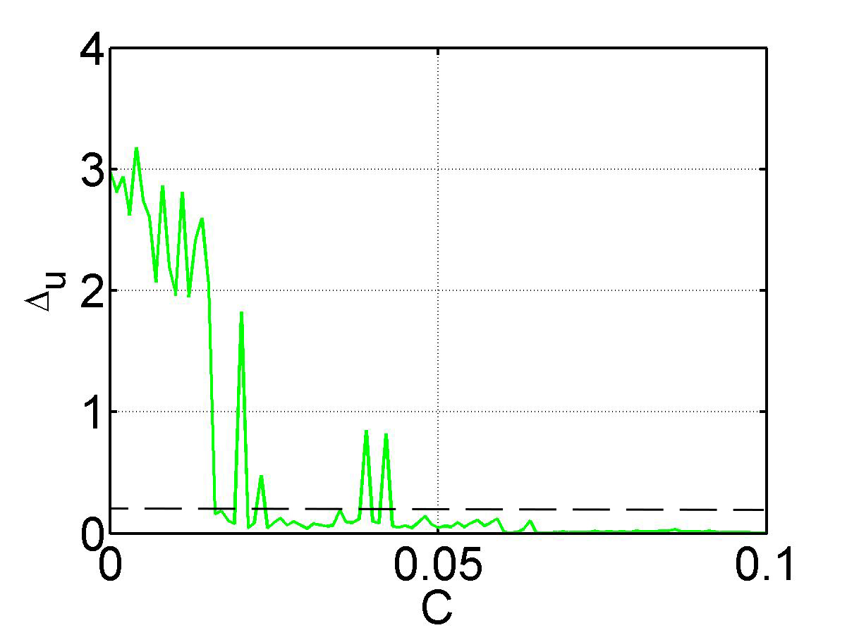
Figure 1: Dependence of the activator synchronization index $\Delta_{u}$ on the coupling strength $C$ for the FitzHugh-Nagumo network given by Eq. (1) with Cantor-type hierarchical topology. The black dashed line indicates the synchrony condition $\Delta_{u}<2\sigma$. Parameters: $B=[1~{}0~{}1]$, $b=3$, $n=4$, $N=82$, $\tau=1.5$, $\varepsilon=0.01$. The threshold parameters $a_{i}$ are normally distributed with mean $\mu=1$ and standard deviation $\sigma=0.1$, truncated at $a_{i}=\mu\pm\sigma$. Initial conditions: $u_{i}(t)=0$, $v_{i}(t)=0$, $i=1,\dots,N$, for $t\in[-\tau,0]$.

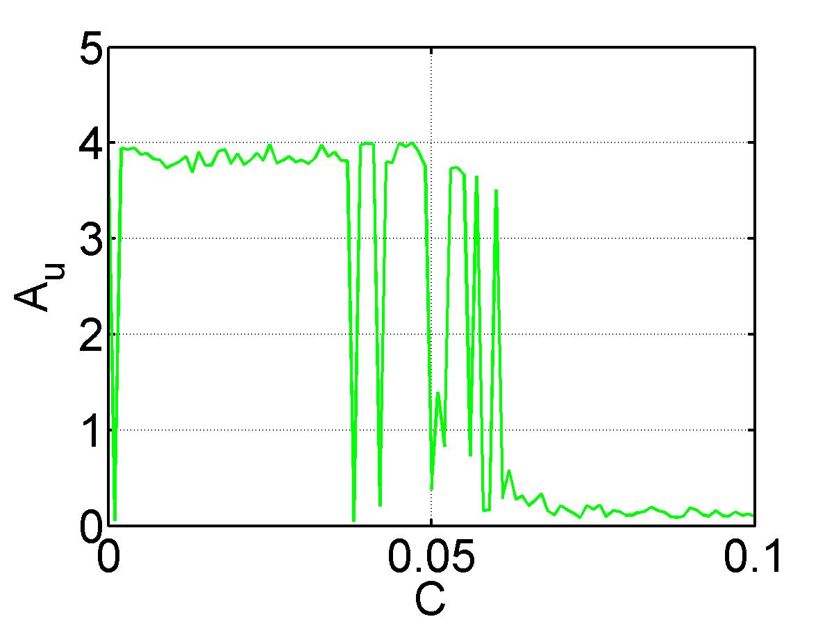
Figure 2: Dependence of the activator oscillation amplitude $A_{u}$ of the first node on the coupling strength $C$ for the FitzHugh-Nagumo network given by Eq. (1) with Cantor-type hierarchical topology. Parameters and initial conditions as in Fig. 1.

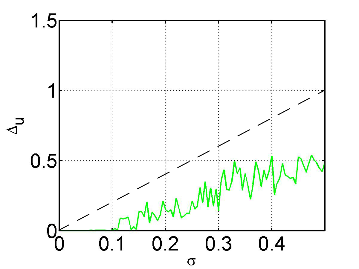
Figure 3: Dependence of the activator synchronization index $\Delta_{u}$ on the standard deviation $\sigma$ of threshold parameters $a_{i}$ for the FitzHugh-Nagumo network given by Eq. (1) with Cantor-type hierarchical topology. The black dashed line indicates the synchrony condition $\Delta_{u}<2\sigma$. Parameters: $C=0.065$. Other parameters and initial conditions as in Fig. 1.

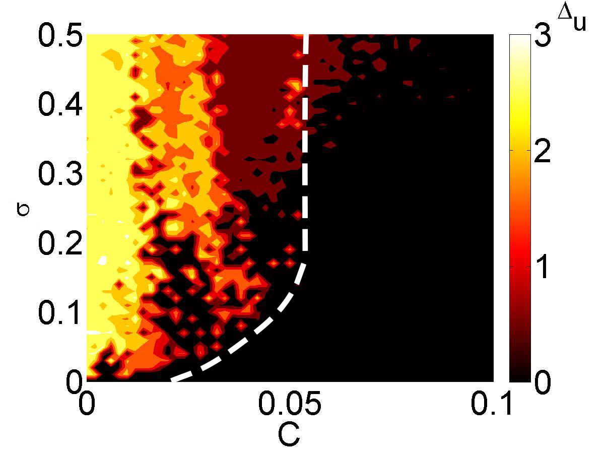
Figure 4: Dependence of the activator synchronization index $\Delta_{u}$ on the coupling strength $C$ and the standard deviation $\sigma$ of threshold parameters $a_{i}$ for the FitzHugh-Nagumo network given by Eq. (1) with Cantor-type hierarchical topology. The white dashed curve indicates the synchrony boundary $\Delta_{u}=2\sigma$. To the right of this curve synchronization holds. Parameters and initial conditions as in Fig. 1.

The simulations were carried out in the Matlab environment using the function $\it dde23$.

In the current study we use as base pattern $B=[1~{}0~{}1]$, i.e., $b=3$. We perform $n=4$ iterations yielding a network of size $N=b^{4}+1=82$ nodes. For this base the value of $c_{1}$ (number of times the symbol $1$ is encountered within the base $B$) equals $2$, i.e., the connectivity matrix has a fractal dimension of $d_{f}=\ln 2/\ln 3=0.6309$. After $n=4$ iterations, each node is connected to $n_{i}=c_{1}^{n}=2^{4}=16$ other nodes, while no connection to the remaining $b^{n}+1-n_{i}=66$ elements exists. From the results obtained in Sec. III.2, we expect the network to synchronize at $C>1/n_{i}=0.0625$.

We now consider a network with a delay $\tau=1.5$ and a standard deviation of $\sigma=0.1$ for the threshold parameters $a_{i}$. We change the coupling strength $C$ from $0$ to $0.1$ and check whether the network synchronizes. To characterize the degree of synchrony, we introduce the activator synchronization index $\Delta_{u}=\max_{i=1}^{N}|u_{i}(t^{*})-\bar{u}(t^{*})+a_{i}-\bar{a}|$, where we define synchrony by the condition $\Delta_{u}<2\sigma$. Here we use $t^{*}=30\geqslant t_{c}$, where $t_{c}$ is the characteristic transient time, to analyze the network after the decay of all transients. The results of the simulation are presented in Fig. 1, where the synchronization index vs. the coupling strength is shown. One can see that there is a critical coupling strength $C^{*}\approx 0.045$, such that for $C>C^{*}$ synchronization holds with some level of precision. To distinguish whether the network is in an oscillatory or excitable state we introduce the activator oscillation amplitude of the first node $A_{u}$ as the difference between the maximum and minimum values of the activator after the transient. Figure 2 shows the dependence of the activator oscillation amplitude of the first node $A_{u}$ on the coupling strength $C$ showing that for $C>0.06$ the $1$st node is in the excitable state. Thus, by combining the results of the simulations shown in Figs. 1 and 2 we conclude that for $0.045<C<0.06$ we obtain synchronization in an oscillatory state. The results of the simulations confirm the idea discussed in Sec. III.3.

Now we fix the delay $\tau=1.5$ and the coupling strength $C=0.065$ and change the standard deviation $\sigma$ from $0$ to $0.5$. The results of the simulation are shown in Fig. 3. As anticipated, the synchronization error increases as $\sigma$ is enlarged. For all $\sigma$ the activator synchronization index is below $2\sigma$ marked by a black dashed line. This is the level of precision of synchronization predicted in Sec. III.2. Note that for $\sigma<0.1$ the activator synchronization index $\Delta_{u}$ is close to zero. To raise the level of precision for $\sigma>0.1$, we can increase the coupling strength $C$.

Figure 4 shows the value of the activator synchronization index $\Delta_{u}$ in the $C$-$\sigma$ plane. The black area corresponds to parameter values where the network synchronizes. The value $C>1/n_{\text{min}}=0.0625$ approximates well the threshold between synchronization and desynchronization as predicted in Sec. III.2. For increasing $\sigma$, $\Delta_{u}$ increases showing that synchronization with less precision takes place.

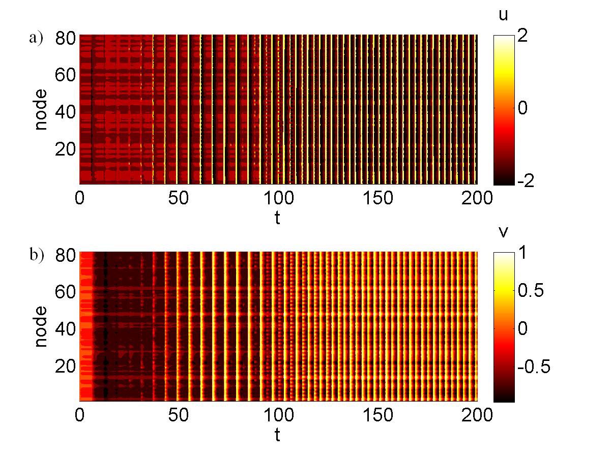
Figure 5: Dynamics of 82 FitzHugh-Nagumo systems given by Eq. (1) with Cantor-type hierarchical topology. (a) and (b): time series of the activator and the inhibitor of all nodes, respectively. Parameters: $C=0.065$, $\tau=6$. Other parameters and initial conditions as in Fig. 1.

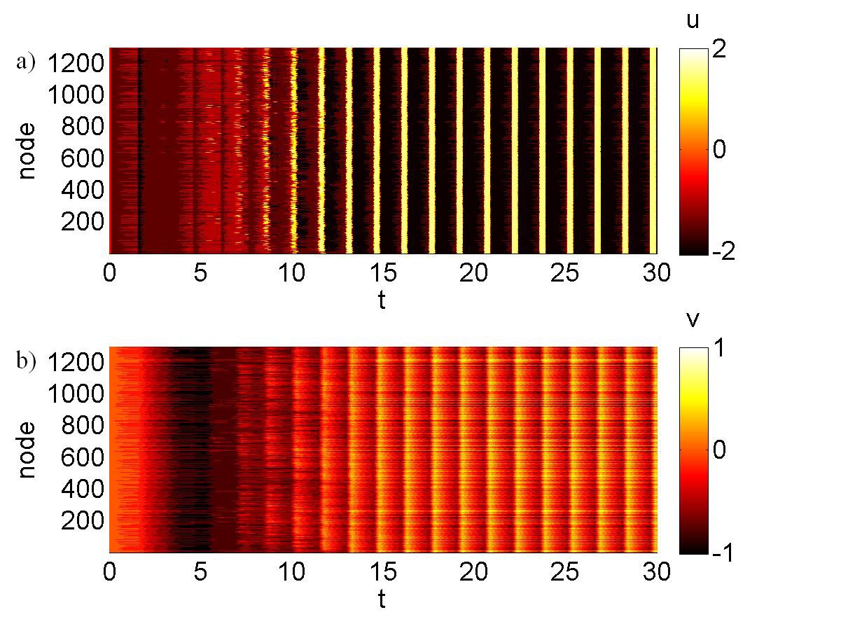
Figure 6: Dynamics of 1297 FitzHugh-Nagumo systems given by Eq. (1) with Cantor-type hierarchical topology. (a) and (b): time series of the activator and the inhibitor of all nodes, respectively. Parameters: $B=[1~{}0~{}1~{}0~{}0~{}0]$, $b=6$, $n=4$, $N=1297$, $C=0.04$. Other parameters and initial conditions as in Fig. 1.

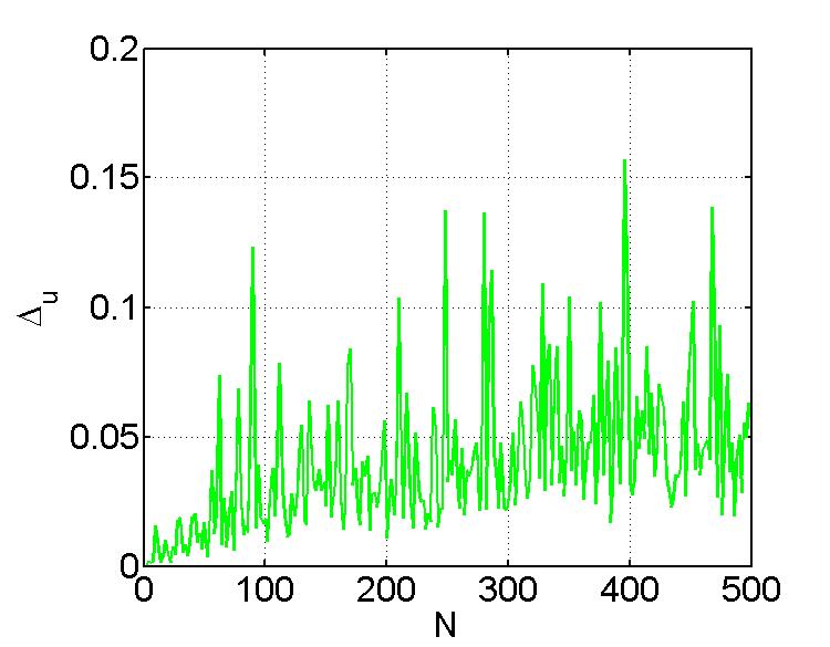
Figure 7: Dependence of the activator synchronization index $\Delta_{u}$ on the number of nodes $N$ for the FitzHugh-Nagumo network given by Eq. (1) with bidirectional ring topology and local coupling, Eq. (26). Parameters: $\tau=1.5$, $\varepsilon=0.01$, $C=1$. The threshold parameters $a_{i}$ are normally distributed with mean $\mu=1$ and standard deviation $\sigma=0.1$. Initial conditions: $u_{i}(t)=0$, $v_{i}(t)=0$, $i=1,\dots,N$, for $t\in[-\tau,0]$.

We now study the influence of the delay $\tau$ on the dynamics of the network. To this end, we fix the coupling strength at $C=0.065$ and the standard deviation at $\sigma=0.1$. For these parameters we always obtain synchronization, however, the delay affects the transient time. For example, for $\tau=6$ the transient time takes approximately $110$ units of time (see Fig. 5). Figure 5a shows that during the transient time, the network already synchronizes but with a lower frequency than the final one. Note that many authors have emphasized the importance of the transient phenomena that arise in neural networks with delay GRO99 ; MIL10 ; MIL12 ; PAK98 ; QUA11 . However, for the chosen parameters we have not observed these phenomena.

Next we consider how synchronization depends on the base pattern $B$. A systematic study of the influence of different base patterns has been performed for networks of identical Van der Pol oscillators in the context of chimera states ULO16 . In agreement with the synchronization condition $C>1/n_{\text{min}}$ (cf. Sec. III.2), the numerical simulations show that synchronization depends only on the number of elements equal to $1$ in each row of the connectivity matrix $\mathbf{G}$. We carry out simulations with different bases of $b=6$ elements with $n=4$ iteration and $c_{1}=2$ nonzero entries, and obtain synchronization in all cases for $C=0.065$. As an example we show in Fig. 6 the results of simulations of the FHN network with $C=0.04$ and the base pattern $B=[1~{}0~{}1~{}0~{}0~{}0]$. Note that for $C=0.065$ and base pattern $B=[1~{}0~{}1~{}0~{}0~{}0]$ there is also synchronization (not shown here), however, the network is in the excitable regime, because the coupling strength is too high for the network to be in the oscillatory regime as discussed in Sec. III.3.

Finally, we investigate how the size of the network influences its synchronizability. Since in the case of hierarchical topologies the number of nodes $N$ is given by $b^{n}+1$ where $b$ is the length of the base and $n$ the number of iterations, the hierarchical network does not allow for increasing $N$ in equally-sized small steps. Therefore, we choose here a bidirectionally locally coupled ring given by the following adjacency matrix

$$\mathbf{G}=\begin{pmatrix}0&1&0&\cdots&1\\ 1&0&1&\cdots&0\\ \vdots&\vdots&\vdots&\ddots&\vdots\\ 0&0&0&\cdots&1\\ 1&0&0&\cdots&0\end{pmatrix}.$$ (26)

Thus, each node has only two (bidirectional) connections for any size of the system. We fix the coupling strength at $C=1$ and the standard deviation at $\sigma=0.1$. For $C=1>1/n_{\text{min}}=0.5$ we expect synchronization (cf. Sec. III.2). The results of the simulation are presented in Fig. 7, where the synchronization index vs. the number of nodes is shown. One can see that $\Delta_{u}<2\sigma$, $\forall N$. This means that the network is synchronized with precision $2\sigma$ for all $N$. We conclude that synchronization does not depend on the network size but only on the coupling strength and the number of connections to each node of the network. Note, however, that the quality of synchronization, i.e., the value of $\Delta_{u}$ slightly depends on the network size.

V Control of synchronization in FitzHugh-Nagumo network

In this section we study how to control synchronization in the case where the synchronization condition $C>1/n_{\text{min}}$ is not met. For this purpose a mean field control, i.e., adding the term $I=\frac{1}{N}\sum_{i=1}^{N}u_{i}$ to each node, has been considered, for example in Refs. ROS04, ; ROS04a, . However, here we suggest a different approach. We will use the control $I(t)$ in the form

$$I(t)=\gamma u(t),$$ (27)

where $\gamma$ is a control gain and $u$ is an activator value of the master system, which is described by the following equations

$$\varepsilon\dot{u} =u-\frac{u^{3}}{3}-v,$$ (28)

$$\dot{v} =u+a$$

where $v$ is an inhibitor value and $a$ is a desired threshold. Compared to a mean field control this approach has the advantage that it is not necessary to measure and average some output variable. Furthermore, even if all oscillators are in the excitable regime the control ensures synchronization in an oscillatory state if we choose $|a|<1$ in Eq. (28).

In the following, we will use $\gamma=0.3$ and $a=0.9$, i.e.,the master system is in the oscillatory regime. We will demonstrate the control in the form Eq. (27) on different network topologies.

V.1 Bidirectional ring topology

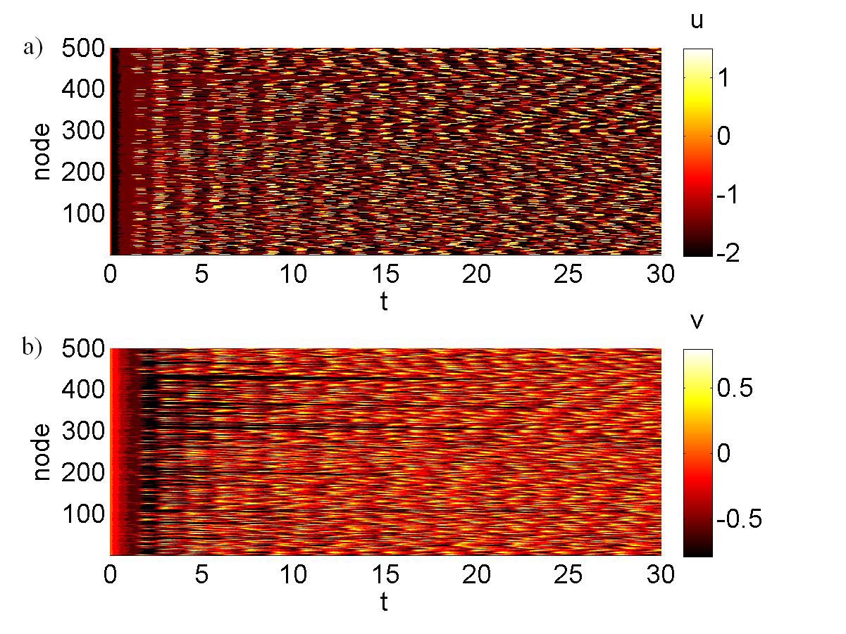
Figure 8: Dynamics of 500 FitzHugh-Nagumo systems given by Eq. (1) with a locally coupled ring topology Eq. (26) without control, i.e., $I(t)=0$. (a) and (b): time series of the activator and the inhibitor of all nodes, respectively. Parameters: $N=500$, $C=0.1$, $\tau=1.5$, $\varepsilon=0.01$. The threshold parameters $a_{i}$ are normally distributed with mean $\mu=1$ and standard deviation $\sigma=0.1$, truncated at $a_{i}=\mu\pm\sigma$. Initial conditions: $u_{i}(t)=0$, $v_{i}(t)=0$, $i=1,\dots,N$, for $t\in[-\tau,0]$.

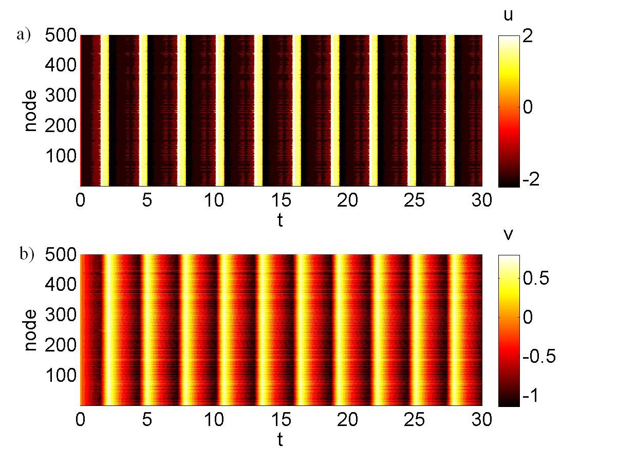
Figure 9: Control of synchronization in 500 FitzHugh-Nagumo systems with a locally coupled ring topology Eq. (26) by the external stimulus $I(t)$ according to Eqs. (27) and (28). (a) and (b): time series of the activator and the inhibitor of all nodes, respectively. Parameters: $\gamma=0.3$, $a=0.9$. Other parameters and initial conditions as in Fig. 8.

We start our consideration with a one-dimensional ring of $N$ delay-coupled FHN oscillators, where each element is coupled to its neighbors on both sides, i.e., the system (1) with the connectivity matrix $\mathbf{G}$ given by Eq.  (26).

For the simulation we consider the case of $N=500$ nodes. We use a coupling strength $C$ equal to $0.1$. Without control the network does not synchronize as can be seen in Fig. 8, where the simulation of a network without control, i.e., $I(t)=0$, is shown. Clearly, there is no synchronization between the activator and inhibitor values.

To synchronize this network we use the control in the form of Eqs. (27) and (28). The result is shown in Figure 9: The control goal is achieved and synchronization holds for the activators (Fig. 9a) and the inhibitors (see Fig. 9b).

V.2 Hierarchical network topology

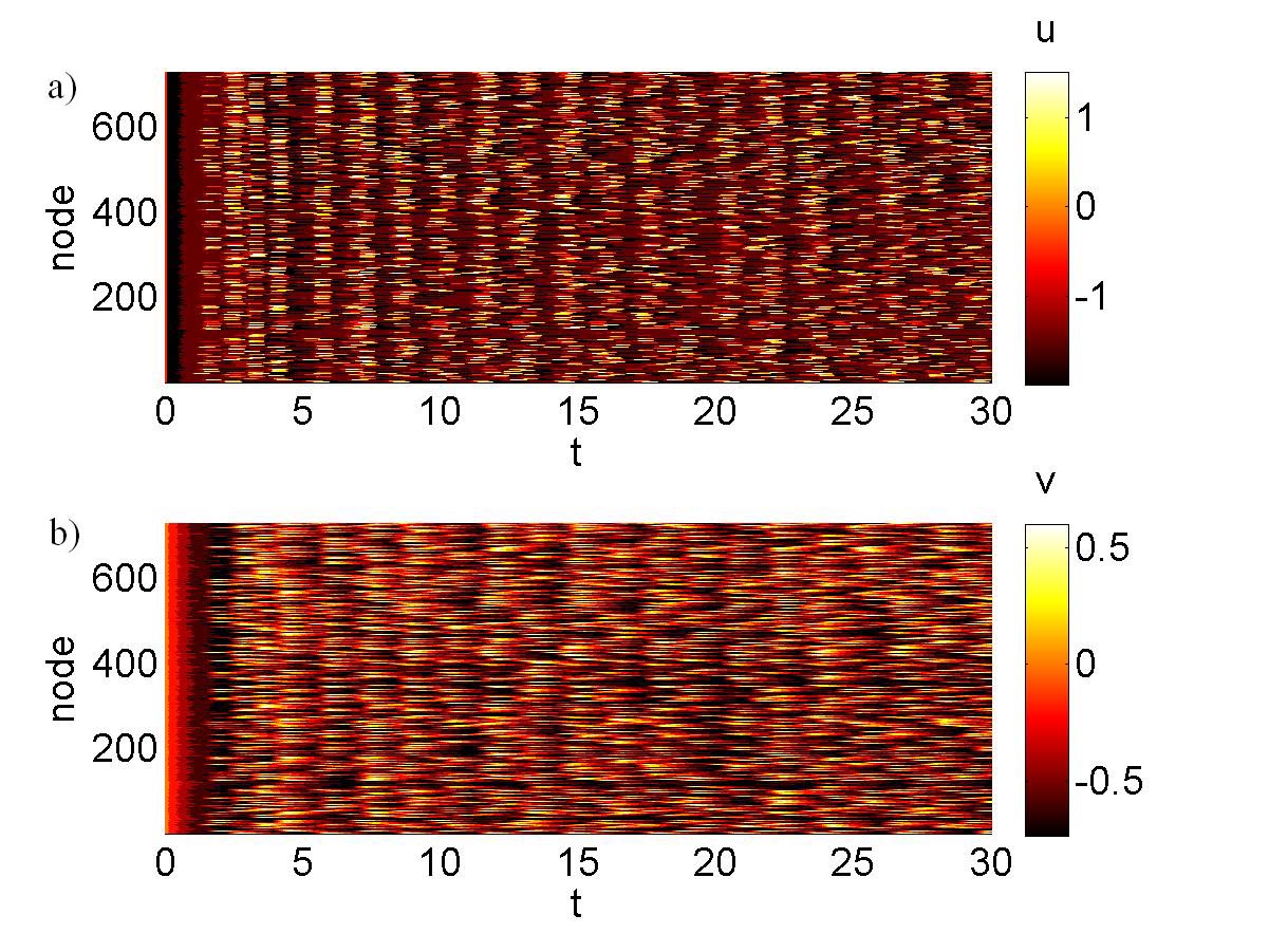
Figure 10: Dynamics of 730 FitzHugh-Nagumo systems with Cantor-type hierarchical topology without control, i.e., $I(t)=0$. (a) and (b): time series of the activator and the inhibitor of all nodes, respectively. Parameters: $n=6$, $N=730$, $C=0.001$. Other parameters and initial conditions as in Fig. 1.

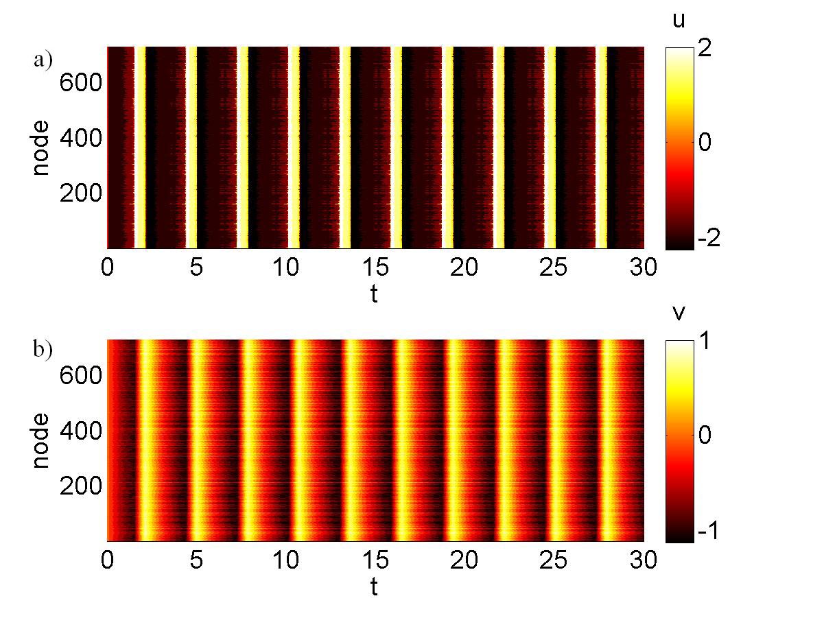
Figure 11: Control of synchronization in 730 FitzHugh-Nagumo systems with Cantor-type hierarchical topology by external stimulus $I(t)$ according to Eqs. (27) and (28). (a) and (b): time series of the activator and the inhibitor of all nodes, respectively. Parameters: $\gamma=0.3$, $a=0.9$. Other parameters and initial conditions as in Fig. 10.

Next we investigate a hierarchical topology with base pattern $B=[1~{}0~{}1]$ and iteration number $n=6$, i.e., the coupling matrix $\mathbf{G}$ has the dimension $N\times N$ with $N=3^{6}+1=730$ (for the construction of a hierarchical network see Sec. IV). We use a very weak coupling strength $C$ equal to $0.001$. Figure 10 shows the results of the simulation of network behavior without control, i.e., $I(t)=0$. Clearly, no synchronization between the nodes takes place.

To synchronize this network we use again the control $I(t)$ given by Eqs. (27) and (28). Figure 11 presents the results of a simulation of the FHN network (1) with hierarchical topology and the external stimulus $I(t)$. The control goal is achieved and synchronization holds (see the time series of the activators and inhibitors in Fig. 11(a), and (b), respectively).

V.3 Random network topology

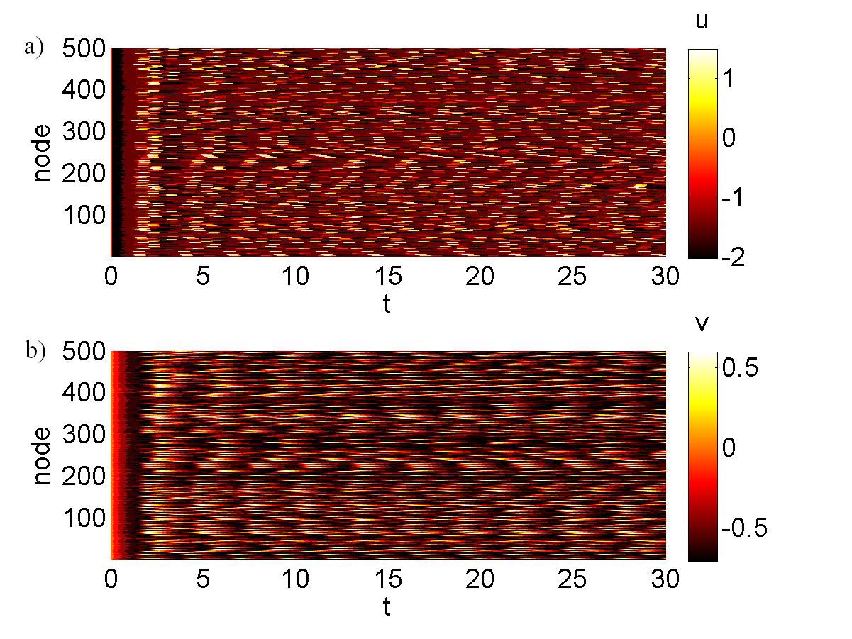
Figure 12: Dynamics of 500 FitzHugh-Nagumo systems with a random topology without control, i.e., $I(t)=0$. (a) and (b): time series of the activator and the inhibitor of all nodes, respectively. Parameters: $N=500$. The nonzero entries are drawn from a Gaussian distribution with mean $\mu_{C}=1$ and variance $\sigma_{C}^{2}=1$, truncated at $a_{i}=\mu\pm\sigma$. Parameters: $C=0.0001$. Other parameters and initial conditions as in Fig. 8.

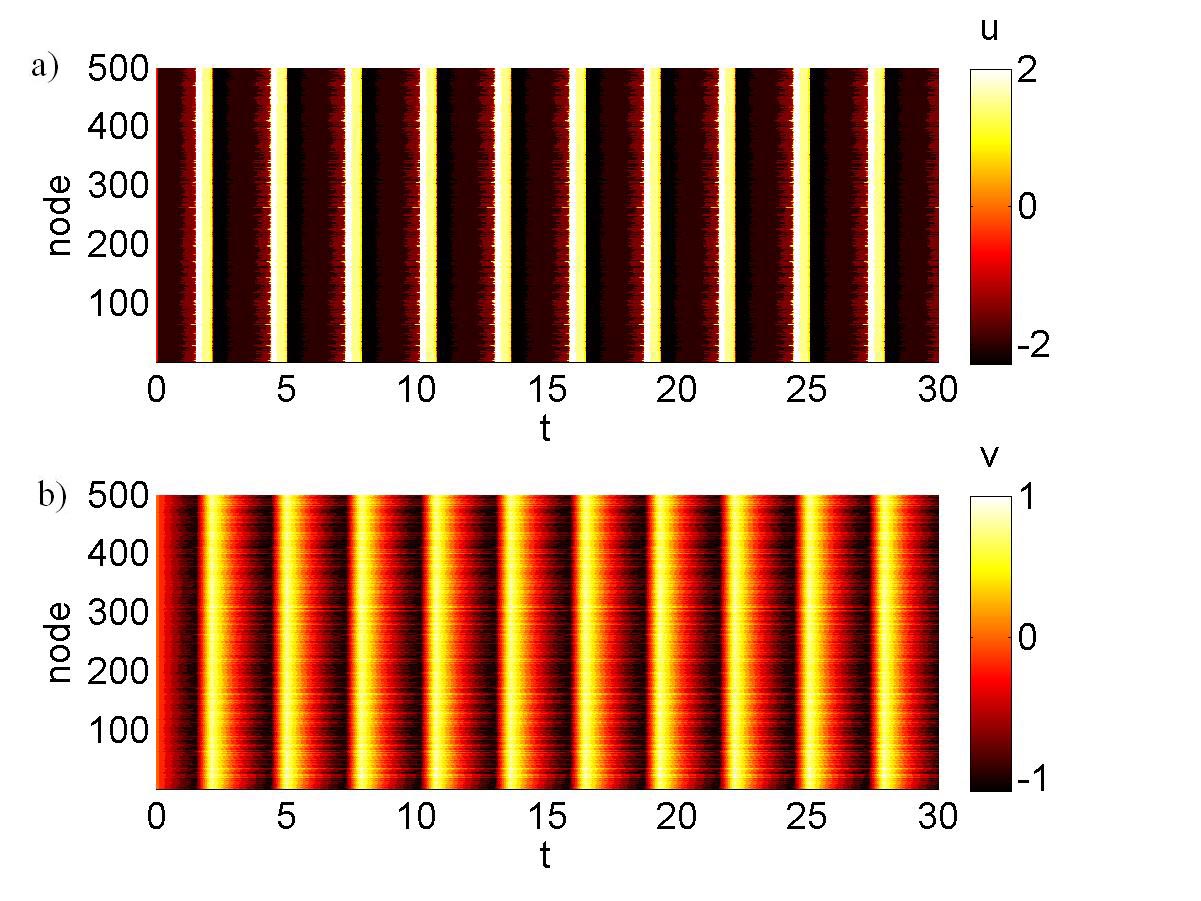
Figure 13: Control of synchronization in 500 FitzHugh-Nagumo systems with a random topology by external stimulus $I(t)$ according to Eqs. (27) and (28). (a) and (b): time series of the activator and the inhibitor of all nodes, respectively. Parameters: $\gamma=0.3$, $a=0.9$. Other parameters and initial conditions as in Fig. 12

Last we consider a network of $N=500$ nodes with random topology. We use a sparse matrix with link density equal to $0.3$. This means there are approximately $0.3N^{2}$ normally distributed nonzero entries. These nonzero entries are drawn from a Gaussian distribution with mean $\mu_{C}=1$ and variance $\sigma_{C}^{2}=1$, truncated at $a_{i}=\mu\pm\sigma$. This process results in a weighted random network. Note that in this case the average node degree is much higher compared to the previously studied topologies. Thus, only for very weak coupling strengths we anticipate non-synchronous dynamics (see Sec. III.2), in which case the need of control arises.

In fact, for $C=0.0001$ no synchronization takes place as can be seen in Fig. (12). Applying the control in the form of Eqs. (27) and (28) synchronizes the network as shown for the activators and inhibitors in Figs. 13(a) and (b), respectively.

VI Conclusion

We have considered synchronization and its control in networks of heterogeneous FitzHugh-Nagumo systems, a neural model which is considered to be generic for excitable systems close to a Hopf bifurcation. To this end, we have investigated networks with heterogeneous threshold parameters. It is well known that networks with heterogeneous nodes are much less likely to synchronize than networks of identical nodes. Furthermore, synchrony will take place in a state where the trajectories of the different nodes are not identical but small deviations can be observed. To counteract this effect of heterogeneity we have proposed an algorithm for controlling synchrony.

First, we have generalized the analytic conditions for the occurrence of the Hopf bifurcations obtained in Refs. SCH08, ; PLO15, for unidirectional locally coupled ring networks. In this way, we have been able to determine the threshold values for which the system is in the excitable regime. Afterwards, we have considered the case that all but one node are in synchrony and derived a critical coupling strength depending on the minimum node degree of the network. Above the critical coupling strength the node will synchronize with the rest of the network. However, if the coupling strength becomes too large, synchronization still holds but amplitude death sets in. Thus, synchronization in an oscillatory state is only possible for intermediate coupling strengths. We have studied synchronization in networks with Cantor-type hierarchical topologies. The study of different hierarchical architectures in the neuron connectivity is motivated by MRI results of the brain structure which shows that the neuron axon network spans the brain area fractally and not homogeneously. The results of these numerical investigations match with our analytical synchronization condition.

Based on the result that the network does not synchronize for too small coupling strengths, we have suggested to add the same external stimulus to all nodes to ensure synchronization in networks where it is absent without control. We have considered the activator value of a master neuron as an external stimulus. We have then applied the control algorithm to different types of networks (bidirectional ring networks, hierarchical networks, random networks), and the simulation results have shown synchronization. Since we use the activator value of the neuron in the oscillatory state, we suppose that it is possible to consider other periodic functions with appropriate frequency as a control to ensure the synchronization, and we have confirmed this in simulations (not shown in the paper). Furthermore, we suggest that our control algorithm and obtianed synchronization conditions can also help with study of desynchronization of the network in cases where this is desirable, for example in the case of abnormal synchrony in the brain as in epilepsy or Parkinson disease. Given the paradigmatic nature of the FitzHugh-Nagumo system, we expect our investigations to be applicable in a wide range of excitable systems, for instance, to the other models for neural spiking WIL99 ; IZH03 ; NAU08 .

- (1) I.I. Blekhman, Synchronization in Science and Technology (ASME Press, 1988).
- (2) A. Pikovsky, M. Rosenblum, and J. Kurths, Synchronization: A universal concept in nonlinear sciences (Cambridge University Press, Cambridge, 2001).
- (3) K. Wiesenfeld, and J.W. Swift, Phys. Rev. E 51, 1020 (1995).
- (4) K. Wiesenfeld et al., Phys. Rev. Lett. 65, 1749 (1990).
- (5) C.S. Peskin, Mathematical Aspects of Heart Physiology (Courant Institute of Mathematical Sciences, New York, 1975).
- (6) J. Buck and E. Buck, Science 159, 1319 (1968).
- (7) T.J. Walker, Science 166, 891 (1969).
- (8) I. Kiss, Y. Zhai, and J. Hudson, Phys. Rev. Lett. 88, 238301 (2002); Science 296, 1676 (2002).
- (9) P.A. Tass, Phase Resetting in Medicine and Biology: Stochastic Modelling and Data Analysis (Springer, Berlin, 1999).
- (10) D. Golomb, D. Hansel, and G. Mato, in Neuro-informatics and Neural Modeling, Handbook of Biological Physics Vol. 4, edited by F. Moss and S. Gielen (Elsevier, Amsterdam, 2001), pp. 887-968.
- (11) Epilepsy as a Dynamic Disease, edited by J. Milton and P. Jung (Springer, Berlin, 2003).
- (12) S.A. Chkhenkeli, Bull. Georgian Acad. Sci. 90, 406 (1978).
- (13) A. Behabid et al., Lancet 337, 403 (1991).
- (14) J. Zhou, J. Lu, and J. Lü, Automatica 44, 996 (2008).
- (15) X. Lu, and B. Qin, Phys. Lett. A 373, 3650 (2009).
- (16) J. Lu, J. Kurths, J. Cao, N. Mahdavi, and C. Huang, IEEE Trans. Neural Netw. Learn. Syst. 23, 285 (2012).
- (17) A.A. Selivanov, J. Lehnert, T. Dahms, P. Hövel, A.L. Fradkov, and E. Schöll, Phys. Rev. E 85, 016201 (2012).
- (18) P.Y. Guzenko, J. Lehnert, and E. Schöll, Cybernetics and Physics 2, 15 (2013).
- (19) J. Lehnert, P. Hövel, A.A. Selivanov, A.L. Fradkov, and E. Schöll Phys. Rev. E 90, 042914 (2014).
- (20) E. Schöll, S.H.L. Klapp, and P. Hövel, Control of Self-Organizing Nonlinear Systems, (Springer, Berlin, 2016).
- (21) S.H. Strogatz, Physica D 143, 1 (2000).
- (22) J. Sun, E.M. Bollt, and T. Nishikawa, Europhys. Lett. 85, 60011 (2009).
- (23) M.G. Rosenblum, A. Pikovsky, Phys. Rev. E 70, 041904 (2004).
- (24) M.G. Rosenblum, A. Pikovsky, Phys. Rev. Lett. 92, 114102 (2004).
- (25) O.V. Popovych,C. Hauptmann, P.A. Tass, Phys. Rev. Lett. 94, 164102 (2005).
- (26) R. FitzHugh, Biophys. J. 1, 445 (1961).
- (27) J. Nagumo, S. Arimoto, and S. Yoshizawa., Proc. IRE 50, 2061 (1962).
- (28) V. Vuksanović, and P. Hövel, NeuroImage 97, 1 (2014).
- (29) P. Katsaloulis, D. A. Verganelakis, and A. Provata, Fractals 17, 181 (2009).
- (30) P. Expert, T.S. Evans, V. D. Blondel, and R. Lambiotte, Proc. Natl. Acad. Sci. U.S.A. 108, 7663 (2011).
- (31) A. Provata, P. Katsaloulis, and D.A Verganelakis, Chaos Soliton. Fract. 45, 174 (2012).
- (32) I. Omelchenko, A. Provata, J. Hizanidis, E. Schöll, and P. Hövel, Phys. Rev. E 91, 022917 (2015).
- (33) B. Lindner, J. García-Ojalvo, A.B. Neiman, and L. Schimansky-Geier, Phys. Rep. 392, 321 (2004).
- (34) M. Heinrich, T. Dahms, V. Flunkert, S.W. Teitsworth, and E. Schöll, New J. Phys. 12, 113030 (2010).
- (35) M. P. Nash, A. V. Panfilov, Prog. Biophys. Mol. Biol. 85, 501 (2004).
- (36) A. T. Winfree, Chaos 1, 303 (1991).
- (37) A. Ganopolski, S. Rahmstorf, , Phys. Rev. Lett. 88, 038501 (2002)
- (38) J.D. Murray, Mathematical Biology, Vol. 19 of Biomathematics Texts, 2nd ed. (Springer, Berlin Heidelberg, 1993).
- (39) E.M. Izhikevich, Int. J. Bifur. Chaos 10, 1171 (2000).
- (40) M.A. Dahlem, G. Hiller, A. Panchuk and E. Schöll, Int. J. Bifur. Chaos 19, 745 (2009).
- (41) E. Schöll, G. Hiller, P. Hövel, and M.A. Dahlem, Phil. Trans. R. Soc. A. 367, 1079 (2009).
- (42) S.A. Plotnikov, J. Lehnert, A.L. Fradkov, and E. Schöll, Int. J. Bifur. Chaos 26, 1650058 (2016).
- (43) P. Katsaloulis, A. Ghosh, A. C. Philippe, A. Provata, and R. Deriche, Eur. Phys. H. B 85, 1 (2012).
- (44) B. B. Mandelbrot, The Fractal Geometry of Nature, 3rd ed. (W. H. Freeman and Comp., New York, 1983).
- (45) J. Feder, Fractals (Plenum Press, New York, 1988).
- (46) C. Grotta-Ragazzo, K. Pakdaman, and C.P. Malta, Phys. Rev. E 60, 6230 (1999).
- (47) J. Milton, P. Naik, C. Chan, and S.A. Campbell, Math. Model. Nat. Phenom. 5, 125 (2010).
- (48) J.G. Milton, Eur. J. Neurosci. 36, 2156 (2012).
- (49) K. Pakdaman, C. Grotta-Ragazzo, C.P. Malta, O. Arino, and J.-F. Vobert, Neural Net. 11, 509 (1998).
- (50) A. Quan, I. Osorio, T. Ohira, and J. Milton, Chaos 21, 047512 (2011).
- (51) S. Ulonska, I. Omelchenko, A. Zakharova, and E. Schöll, arXiv:1603.00171 (2016).
- (52) H.R. Wilson, J. Theor. Biol. 200, 375 (1999).
- (53) E.M. Izhikevich, IEEE Trans. Neural Net. 14, 1569 (2003).
- (54) R. Naud, N. Marcille, C. Clopath, W. Gerstner, Biol. Cybern. 99, 335 (2008).