Optimal Caching and User Association in Cache-enabled Heterogeneous Wireless Networks

Abstract

Heterogenous wireless networks (Hetnets) provide a powerful approach to meet the massive growth in traffic demands, but also impose a significant challenge on backhaul. Caching at small base stations (BSs) and wireless small cell backhaul have been proposed as attractive solutions to address this new challenge. In this paper, we consider the optimal caching and user association to minimize the total time to satisfy the average demands in cached-enabled Hetnets with wireless backhaul. We formulate this problem as a mixed discrete-continuous optimization for given bandwidth and cache resources. First, we characterize the structure of the optimal solution. Specifically, we show that the optimal caching is to store the most popular files at each pico BS, and the optimal user association has a threshold form. We also obtain the closed-form optimal solution in the homogenous scenario of pico cells. Then, we analyze the impact of bandwidth and cache resources on the minimum total time to satisfy the average demands. Finally, using numerical simulations, we verify the analytical results.

I Introduction

The rapid proliferation of smart mobile devices has triggered an unprecedented growth of the global mobile data traffic. Heterogenous wireless networks (Hetnets) have been proposed as an effective way to meet the dramatic traffic growth by deploying short range small base stations (BSs) together with traditional macro BSs [1]. Significant increase in network capacity is possible mainly because the small cells can operate simultaneously, providing better time or frequency reuse. However, this approach imposes a significant challenge of providing expensive high-speed backhaul links for connecting all the small BSs to the core network. The backhaul capacity requirement can be enormously high during peak traffic hours.

Caching at small BSs is a promising approach to alleviate the backhaul capacity requirement in Hetnets. Many existing works have focused on optimal cache placement at small BSs, which is of critical importance in cache-enabled Hetnets. For example, [2] and [3] consider caching at small BSs in a single macro cell with multiple small cells where the coverage areas of small cells are overlapping. File requests which cannot be satisfied locally at small BSs are served by the macro BS. Specifically, in [2], the authors consider the optimal caching design to minimize the expected delay for downloading uncached files from the macro BS. In [3], the authors consider the optimal caching to minimize the requests served by the macro BS. The optimization problems in [2] and [3] are NP-hard, and simplified caching solutions are proposed with approximation guarantees.

Backhaul limitation is a critical problem in Hetnets. In [4, 5, 6, 7], the authors consider caching at small BSs in Hetnets with backhaul constraints. Small BSs retrieve uncached files via wireline backhaul from the core network and then transmit to local users. Thus, the service rate of uncached files at small BSs is also limited by the backhaul capacity. Specifically, [4, 5, 6] consider caching the most popular files at each small BS and focuses on analyzing the network performance. [7] considers least frequently used caching policy and studies the optimal user association. Wireless backhaul is an attractive option for small BSs in Hetnets as it is easier to deploy and is more cost effective than fiber based backhaul. When wireless backhaul is considered, it is essential to optimally allocate time or frequency resources between wireless backhaul for file retrievements and small BSs for file transmissions.

To avoid inter-tier interference and increase the spatial reuse in Hetnets, the well known techniques of intercell interference coordination using almost blanking subframes (ABS slots) and cell range expansion (CRE) have been developed. The joint optimization of ABS slots and CRE in a dynamic traffic scenario has been studied in [8], without considering cache resource and backhaul limitation. In cache-enabled Hetnets with wireless backhaul, caching, ABS slots and CRE should be jointly optimized under wireless backhaul constraints, in order to fully exploit the bandwidth and cache resources to improve network capacity. Note that CRE is not considered in [2], [3], and optimal caching is not studied in [4] and [7]. In this paper, we consider the joint optimization of caching, ABS slots and CRE in a cache-enabled Hetnet consisting of a single macro cell containing multiple pico BSs with wireless backhaul. We formulate a mixed discrete-continuous optimization of the caching and user association to minimize the total time to satisfy the average demands in a dynamic traffic scenario. Note that the user association reflects control of ABS slots and CRE. We show that the optimal caching is to store the most popular files at each pico BS, and the optimal user association for both cached and uncached files has a threshold form resulting in two pico serving regions. The pico serving region for cached files is larger and contains the pico serving region for uncached files. Both ranges are adaptive to the traffic density, cache resource and bandwidth resource. The range difference comes from the difference in backhaul consumption. We also obtain the closed-form optimal solution in the homogenous scenario of pico cells. Then, we analyze the impact of bandwidth and cache resources on the minimum total time to satisfy the average demands. Finally, using numerical simulations, we verify the analytical results.

II System Model

We consider a cache-enabled Hetnet consisting of a single macro cell containing $L\in\mathbb{N}_{+}$ pico BSs, as illustrated in Fig. 1. Let $\mathcal{L}\triangleq\{1,2,\cdots,L\}$ denote the set of $L$ pico BSs. Let $\mathcal{K}\subset\mathbb{R}^{2}$ denote the (compact) coverage area of the macro BS, while $\mathcal{K}_{l}\subset\mathcal{K}$, $l\in\mathcal{L}$ denote the respective coverage areas of the pico BSs. The pico BS coverage areas are assumed disjoint such that a user at a location in $\mathcal{K}_{l}$ can obtain service from both the macro BS and the pico BS $l$. Let $\mathcal{K}_{0}\triangleq\mathcal{K}-\cup_{l=1}^{L}\mathcal{K}_{l}$ denote the set of locations not covered by any pico BS. Any user at a location in $\mathcal{K}_{0}$ will obtain all its support from the macro BS.

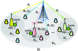
Figure 1: System model.

Let $\mathcal{N}\triangleq\{1,\cdots,N\}$ denote the set of $N$ files (contents) in the network. For ease of illustration, we assume that all files have the same size. All the files are available at the macro BS. Each pico BS $l$ is equipped with a cache, which can store $C_{l}\in\{0,1,\cdots,N\}$ files. Denote $\mathbf{C}\triangleq(C_{l})_{l\in\mathcal{L}}$. Let $s_{l,n}\in\{0,1\}$ represent the caching state for file $n$ at pico BS $l$, where $s_{l,n}=1$ if file $n$ is cached at pico BS $l$, and $s_{l,n}=0$ otherwise. Denote $\mathbf{s}_{l}\triangleq(s_{l,n})_{n\in\mathcal{N}}$. Note that $\mathbf{s}_{l}$ satisfies $\sum_{n=1}^{N}s_{l,n}\leq C_{l}$. For ease of illustration, we assume each pico BS $l$ can retrieve uncached files from the macro BS via a wireless backhaul. Note that our formulation and solution hold when pico BSs retrieve uncached files from any connection point to the core network.

Users want to download files from the network. We assume that the file popularity distribution $\mathbf{p}\triangleq(p_{n})_{n\in\mathcal{N}}$ is identical among all users and is known apriori, where $p_{n}\in[0,1]$ is the popularity of file $n$ and $\mathbf{p}$ satisfies $\sum_{n\in\mathcal{N}}p_{n}=1$. In addition, without loss of generality, we assume $p_{1}\geq p_{2}\ldots\geq p_{N}$. We assume that file requests arrive as a Poisson process with arrival rate $\lambda_{S}$ files/sec and that an arrival is for file $n$ with probability $p_{n}$. The locations of the arrivals are chosen independently at random according to a continuous density $\eta(d\xi)$ with support on $\mathcal{K}$ and bounded uniformly away from 0. Users remain fixed at their initial locations until they obtain their files. Hence, the expected number of requests per second at the vicinity of a point $\xi\in\mathcal{K}$ is given by $\lambda(d\xi)=\lambda_{S}\times\eta(d\xi)$.

The macro BS is assumed to use a much higher transmit power than the pico BSs, to allow it to provide full coverage of the region $\mathcal{K}$. We will therefore only consider control policies in which macro time and pico times are disjoint, to avoid excessive interference at the users from the macro BS when being served by pico BSs. During macro time, the macro BS can transmit to a user or a pico BS. On the other hand, pico BSs are spatially separated and use much lower power. We will therefore consider control policies in which the pico BSs are allowed to operate simultaneously during pico time. Let the time allocated to the pico cells be denoted by $f$ seconds.

The transmission rate of a user is determined by the transmitting BS and the user’s fixed location $\xi$. All locations are in the macro BS coverage area, and the corresponding rate provided by the macro BS to location $\xi\in\mathcal{K}$, if scheduled, is $R_{0}(\xi)$ file/sec/Hz. If the location is within the coverage area of pico BS $l$, then an alternative rate provided by pico BS $l$ to location $\xi\in\mathcal{K}_{l}$, if scheduled, is $R_{l}(\xi)$ file/sec/Hz. Assume that rates depend continuously on location with $0<R_{l,\min}\leq R_{l}(\xi)\leq R_{l,\max}$ for pico cell rates, where $\xi\in\mathcal{K}_{l}$ and $l\in\mathcal{L}$, and with $0<R_{0,\min}\leq R_{0}(\xi)\leq R_{0,\max}$ for the macro cell rates, where $\xi\in\mathcal{K}$. In addition, the rate of the wireless backhaul from the macro BS to pico BS $l$, if scheduled, is $B_{l}$ file/sec/Hz. Since a pico BS has a much larger receive antenna gain than a user, we assume $R_{0}(\xi)<B_{l}$ for all $\xi\in\mathcal{K}_{l}$ and $l\in\mathcal{L}$. The total bandwidth is $W>0$ Hz.

Note that any user at a location in $\mathcal{K}_{0}$ is only served by the macro BS during macro time. A user at a location in $\mathcal{K}_{l}$ can receive a file together from the macro BS and pico BS $l$ during macro time and pico time, respectively. Consider location $\xi\in\mathcal{K}_{l}$ in the coverage area of pico BS $l$. Let $x_{l,n}(\xi)\in[0,1]$ denote the fraction of file $n$ delivered by pico BS $l$ to location $\xi\in\mathcal{K}_{l}$ at rate $R_{l}(\xi)$ during pico time. If file $n$ is not stored at pico BS $l$, i.e., $s_{l,n}=0$, then this $x_{l,n}(\xi)$ fraction of file $n$ has to be first delivered from the macro BS to pico BS $l$ at rate $B_{l}$ via the wireless backhaul during macro time; otherwise, the delivery of this $x_{l,n}(\xi)$ fraction of file $n$ will not consume macro time. The remaining $1-x_{l,n}(\xi)$ fraction of file $n$ will be delivered by the macro BS to location $\xi\in\mathcal{K}_{l}$ at rate $R_{0}(\xi)$ during macro time. Denote $\mathbf{x}_{l}(\xi)\triangleq(x_{l,n}(\xi))_{n\in\mathcal{N}}$ for all $\xi\in\mathcal{K}_{l}$ and $l\in\mathcal{L}$. Note that association $\{\mathbf{x}_{l}(\xi):\xi\in\mathcal{K}_{l},l\in\mathcal{L},\}$ reflects control of ABS slots and CRE.

III Problem Formulation

The time that the HetNet must be active in order to satisfy given traffic demands is an important performance metric. Our goal is to find the optimal pico time $f^{*}$, caching $\{\mathbf{s}_{l}^{*}:l\in\mathcal{L}\}$ and association $\{\mathbf{x}_{l}^{*}(\xi):\xi\in\mathcal{K}_{l},l\in\mathcal{L}\}$ to minimize the total time that the HetNet must be active in order to satisfy the average requests, under given system resources, i.e., bandwidth resource $W$ and cache resource $\mathbf{C}$.

Problem 1 (Optimal Caching and Scheduling)

$$\tau^{*}=\min_{\begin{subarray}{c}f,\{\mathbf{s}_{l}:l\in\mathcal{L}\},\\ \{\mathbf{x}_{l}(\xi):\xi\in\mathcal{K}_{l},l\in\mathcal{L}\}\end{subarray}}\ f+\sum_{n=1}^{N}\int_{\mathcal{K}_{0}}\frac{1}{WR_{0}(\xi)}p_{n}\lambda(d\xi)$$

$$+\sum_{l=1}^{L}\sum_{n=1}^{N}\int_{\mathcal{K}_{l}}\frac{1-x_{l,n}(\xi)}{WR_{0}(\xi)}p_{n}\lambda(d\xi)$$

$$+\sum_{l=1}^{L}\sum_{n=1}^{N}\int_{\mathcal{K}_{l}}\frac{(1-s_{l,n})x_{l,n}(\xi)}{WB_{l}}p_{n}\lambda(d\xi)$$

$$s.t.\quad \sum_{n=1}^{N}\int_{\mathcal{K}_{l}}\frac{x_{l,n}(\xi)}{WR_{l}(\xi)}p_{n}\lambda(d\xi)\leq f,\quad l\in\mathcal{L}$$

$$0\leq x_{l,n}(\xi)\leq 1,\quad l\in\mathcal{L},\ n\in\mathcal{N}$$

$$s_{l,n}\in\{0,1\},\quad l\in\mathcal{L},\ n\in\mathcal{N}$$

$$\sum_{n=1}^{N}s_{l,n}\leq C_{l},\quad l\in\mathcal{L}.$$

Note that $\sum_{n=1}^{N}\int_{\mathcal{K}_{0}}\frac{1}{WR_{0}(\xi)}p_{n}\lambda(d\xi)=\int_{\mathcal{K}_{0}}\frac{1}{WR_{0}(\xi)}\lambda(d\xi)\triangleq\tau_{0}$ represents the macro time to satisfy the average requests from $\mathcal{K}_{0}$, $\sum_{n=1}^{N}\int_{\mathcal{K}_{l}}\frac{1-x_{l,n}(\xi)}{WR_{0}(\xi)}p_{n}\lambda(d\xi)$ represents the macro time to directly satisfy the average requests from $\mathcal{K}_{l}$, while $\sum_{n=1}^{N}\int_{\mathcal{K}_{l}}\frac{(1-s_{l,n})x_{l,n}(\xi)}{WB_{l}}p_{n}\lambda(d\xi)$ represents the macro time to satisfy the average requests from $\mathcal{K}_{l}$ indirectly, by first delivering the uncached files to pico BS $l$ via the wireless backhaul. $\sum_{n=1}^{N}\int_{\mathcal{K}_{l}}\frac{x_{l,n}(\xi)}{WR_{l}(\xi)}p_{n}\lambda(d\xi)$ represents the pico time to satisfy the average requests from $\mathcal{K}_{l}$. If pico BS $l$ carries all the average requests from $\mathcal{K}_{l}$, then it needs time $\bar{f}_{l}\triangleq\sum_{n=1}^{N}\int_{\mathcal{K}_{l}}\frac{1}{WR_{l}(\xi)}p_{n}\lambda(d\xi)=\int_{\mathcal{K}_{l}}\frac{1}{WR_{l}(\xi)}\lambda(d\xi)$. The maximum of such time over all pico BSs is $\bar{f}\triangleq\max_{l\in\mathcal{L}}\bar{f}_{l}$.

Problem 1 is one in the calculus of variations over function $x_{l,n}(\xi)\in[0,1]$, $l\in\mathcal{L}$, $n\in\mathcal{N}$. It also has a continuous variable $f\geq 0$ and $LN$ discrete variables $s_{l,n}\in\{0,1\}$, $l\in\mathcal{L}$, $n\in\mathcal{N}$. Note that the space of $x_{l,n}(\xi)\in[0,1]$, $l\in\mathcal{L}$, $n\in\mathcal{N}$ is compact, $f\geq 0$ can be taken no greater than $\bar{f}$, i.e., $f\in[0,\bar{f}]$, without affecting the optimality. In addition, the space of $s_{l,n}\in\{0,1\}$, $l\in\mathcal{L}$, $n\in\mathcal{N}$ is finite, and the map from $x_{l,n}(\xi)\in[0,1]$, $l\in\mathcal{L}$, $n\in\mathcal{N}$ and $f\in[0,\bar{f}]$ to the objective function in Problem 1 is continuous for any $s_{l,n}\in\{0,1\}$, $l\in\mathcal{L}$, $n\in\mathcal{N}$. Therefore, the minimum is achieved.

Using decomposition, Problem 1 can be equivalently transformed into the following master problem with $L$ subproblems.

Problem 2 (Master Problem of Problem 1)

$$\tau^{*}=\min_{f}\quad \tau(f)$$

$$s.t.\quad f\geq 0$$

where $\tau(f)\triangleq f+\tau_{0}+\sum_{l=1}^{L}\tau_{l}(f)$ and $\tau_{l}(f)$ is given by the optimal value of Subproblem $l$ for given $f\geq 0$.

Problem 3 (Subproblem $l$ of Problem 1)

For $f\geq 0$,

$$\tau_{l}(f)=\min_{\begin{subarray}{c}\mathbf{s}_{l},\\ \{\mathbf{x}_{l}(\xi):\xi\in\mathcal{K}_{l}\}\end{subarray}}\quad \sum_{n=1}^{N}\int_{\mathcal{K}_{l}}\frac{1-x_{l,n}(\xi)}{WR_{0}(\xi)}p_{n}\lambda(d\xi)$$

$$+\sum_{n=1}^{N}\int_{\mathcal{K}_{l}}\frac{(1-s_{l,n})x_{l,n}(\xi)}{WB_{l}}p_{n}\lambda(d\xi)$$

$$s.t.\quad \sum_{n=1}^{N}\int_{\mathcal{K}_{l}}\frac{x_{l,n}(\xi)}{WR_{l}(\xi)}p_{n}\lambda(d\xi)\leq f$$ (1)

$$0\leq x_{l,n}(\xi)\leq 1,\quad n\in\mathcal{N}$$ (2)

$$s_{l,n}\in\{0,1\},\quad n\in\mathcal{N}$$ (3)

$$\sum_{n=1}^{N}s_{l,n}\leq C_{l}.$$ (4)

Note that $\tau_{0}$ denotes the macro time to satisfy the average requests from $\mathcal{K}_{0}$ and $\tau_{l}(f)$ denotes the optimal macro time to satisfy the average requests from $\mathcal{K}_{l}$ directly and indirectly, given that the pico time is no greater than $f$. Therefore, $\tau(f)$ represents the total time to satisfy the average requests in the HetNet given that the pico time is no greater than $f$.

Problem 3 for pico BS $l$ is a mixed discrete continuous optimization. Similarly, it can be easily verified that the minimum is achieved. Problem 2 is a continuous optimization problem over a single variable $f\geq 0$. Later, we shall show that Problem 2 is convex.

IV Optimality Properties

IV-A Optimal Solution

In this part, we characterize the optimal solution to Problem 1. We first characterize the optimal solution to the subproblem for pico BS $l$ in Problem 3 for any given $f\geq 0$. Then, we characterize the optimal solution to Problem 2.

To solve Problem 3, we first solve the continuous relaxation of Problem 3 where $s_{l,n}\in\{0,1\}$ is relaxed to $s_{l,n}\in[0,1]$. We show that the optimal solution to the relaxed problem satisfies $s_{l,n}\in\{0,1\}$, and hence it is also the optimal solution to Problem 3. Define $\rho_{l}(\xi,s)\triangleq\frac{R_{l}(\xi)}{R_{0}(\xi)}-\frac{(1-s)R_{l}(\xi)}{B_{l}}$ ($\xi\in\mathcal{K}_{l}$), $\underline{\rho_{l}}\triangleq\inf\{\rho_{l}(\xi,0):\xi\in\mathcal{K}_{l}\}$, $\bar{\rho_{l}}\triangleq\sup\{\rho_{l}(\xi,1):\xi\in\mathcal{K}_{l}\}$, $\mathcal{A}_{l}(\rho,s)\triangleq\{\xi\in\mathcal{K}_{l}:\rho_{l}(\xi,s)>\rho\}$, and $S_{C_{l}}\triangleq\sum_{n=1}^{C_{l}}p_{n}$. Note that $\mathcal{A}_{l}(\rho,0)\subseteq\mathcal{A}_{l}(\rho,1)\subseteq\mathcal{K}_{l}$. Suppose $\int_{\mathcal{A}_{l}(\rho,s)}d\xi$ is continuous in $\rho$.

Lemma 1

For any given $f\geq 0$, the optimal solution to Problem 3 is given by

$$s_{l,n}^{*}= \begin{cases}1,&n=1,\cdots,C_{l}\\ 0,&\text{otherwise}\end{cases}$$ (5)

$$x_{l,n}^{*}(\xi,f)= \begin{cases}1,&\rho_{l}(\xi,s_{l,n}^{*})>\rho_{l}(f)\\ 0,&\text{otherwise}\end{cases}$$ (6)

where $\rho_{l}(f)$ satisfies

$$S_{C_{l}}\int_{\mathcal{A}_{l}(\rho_{l}(f),1)}\frac{1}{WR_{l}(\xi)}\lambda(d\xi)$$

$$+(1-S_{C_{l}})\int_{\mathcal{A}_{l}(\rho_{l}(f),0)}\frac{1}{WR_{l}(\xi)}\lambda(d\xi)=f$$ (7)

if $f\leq\bar{f}_{l}$, and $\rho_{l}(f)=0$ otherwise. In addition, the optimal value of Problem 3 is given by

$$\tau_{l}(f)= S_{C_{l}}\int_{\mathcal{K}_{l}-\mathcal{A}_{l}(\rho_{l}(f),1)}\frac{1}{WR_{0}(\xi)}\lambda(d\xi)$$

$$+(1-S_{C_{l}})\int_{\mathcal{K}_{l}-\mathcal{A}_{l}(\rho_{l}(f),0)}\frac{1}{WR_{0}(\xi)}\lambda(d\xi)$$

$$+(1-S_{C_{l}})\int_{\mathcal{A}_{l}(\rho_{l}(f),0)}\frac{1}{WB_{l}}\lambda(d\xi).$$ (8)

Proof:

Please refer to Appendix A. ∎

Remark 1 (Optimal Structure)

For any given pico time $f\geq 0$, the optimal caching is to cache the most popular $C_{l}$ files. Thus, $S_{C_{l}}$ reflects the cache hit probability. Given pico time $f\geq 0$, the optimal association $x_{l,n}^{*}(\xi,f)$ takes the threshold form where the threshold $\rho_{l}(f)$ depends on the pico time $f$. Note that $\rho_{l}(f)$ also depends on $W$ and $C_{l}$, which are assumed to be fixed for now. The impact of $W$ and $C_{l}$ on $\rho_{l}(f)$ will be studied later in Section IV-B. Specifically, for any cached file $n=1,\cdots,C_{l}$, the optimal association $x_{l,n}^{*}(\xi,f)=1$ if $\rho_{l}(\xi,1)>\rho_{l}(f)$; for any uncached file $n=C_{l}+1,\cdots,N$, the optimal association $x_{l,n}^{*}(\xi,f)=1$ if $\rho_{l}(\xi,0)>\rho_{l}(f)$. In other words, the threshold $\rho(f)$ determines two pico serving regions $\mathcal{A}_{l}(\rho_{l}(f),1)\subseteq\mathcal{K}_{l}$ and $\mathcal{A}_{l}(\rho_{l}(f),0)\subseteq\mathcal{K}_{l}$ for the cached files and uncached files, respectively, where $\mathcal{A}_{l}(\rho_{l}(f),0)\subseteq\mathcal{A}_{l}(\rho_{l}(f),1)$. For any cached file $n=1,\cdots,C_{l}$, the optimal association $x_{l,n}^{*}(\xi,f)=1$ if $\xi\in\mathcal{A}_{l}(\rho_{l}(f),1)$; for any uncached file $n=C_{l}+1,\cdots,N$, the optimal association $x_{l,n}^{*}(\xi,f)=1$ if $\xi\in\mathcal{A}_{l}(\rho_{l}(f),0)$. Each pico BS is more willing to serve requests for cached files, as no macro time is consumed for fetching these files from the macro BS via wireless backhaul.

From Lemma 1, we have the following corollary.

Corollary 1

When $f=0$ (no pico time), we have $x_{l,n}^{*}(\xi,f)=0$ for all $\xi\in\mathcal{K}_{l}$ and $\tau_{l}(f)=\int_{\mathcal{K}_{l}}\frac{1}{WR_{0}(\xi)}\lambda(d\xi)$. When $f\geq\bar{f}_{l}$, we have $x_{l,n}^{*}(\xi,f)=1$ for all $\xi\in\mathcal{K}_{l}$ and $\tau_{l}(f)=(1-S_{C_{l}})\int_{\mathcal{K}_{l}}\frac{1}{WB_{l}}\lambda(d\xi)$.

Note that $\bar{f_{l}}$ can be interpreted as the largest pico time needed for pico BS $l$ to satisfy the average requests from $\mathcal{K}_{l}$. When $f\in[0,\bar{f_{l}}]$, $\rho_{l}(f)$ satisfying (7) is strictly decreasing in $f$. Thus, when $f\in[0,\bar{f_{l}}]$, $\tau_{l}(f)$ given by (8) is strictly decreasing in $f$. When $f>\bar{f_{l}}$, $\rho_{l}(f)=0$ and $\tau_{l}(f)=(1-S_{C_{l}})\int_{\mathcal{K}_{l}}\frac{1}{WB_{l}}\lambda(d\xi)$, which is the average macro time to satisfy the average requests from $\mathcal{K}_{l}$ indirectly, and does not change with $f$. In addition, by the structure of Problem 3, we can easily see that $\tau_{l}(f)$ is convex over $f$.

Next, we characterize the optimal solution to Problem 2. Based on the properties of $\tau_{l}(f)$ discussed above, we know that $\tau(f)=f+\tau_{0}+\sum_{l=1}^{L}\tau_{l}(f)$ is strictly convex in $f$ over $[0,\bar{f}]$, and is strictly increasing in $f$ when $f>\bar{f}$. Then, we have the following lemma.

Lemma 2

The optimal solution $f^{*}$ to Problem 2 exists and is unique. In addition, $f^{*}$ satisfies: if $\sum_{l=1}^{L}\bar{\rho_{l}}\leq 1$, $f^{*}=0$ (no pico time) is optimal; $\sum_{l=1}^{L}\rho_{l}(\bar{f})\geq 1$, $f^{*}=\bar{f}$ (all pico time) is optimal; otherwise, $f^{*}\in(0,\bar{f})$ satisfies $\sum_{l=1}^{L}\rho_{l}(f^{*})=1$, where $\rho_{l}(f)$ is given by Lemma 1.

Proof:

Please refer to Appendix B. ∎

Based on Lemma 1 and Lemma 2, we characterize the optimal solution to Problem 1 in the following theorem.

Theorem 1

The optimal solution to Problem 1 is given by

$$s_{l,n}^{*}= \begin{cases}1,&n=1,\cdots,C_{l}\\ 0,&\text{otherwise}\end{cases}$$ (9)

$$x_{l,n}^{*}(\xi)= \begin{cases}1,&\rho_{l}(\xi,s_{l,n}^{*})>\rho_{l}(f^{*})\\ 0,&\text{otherwise}\end{cases}$$ (10)

where $f^{*}$ given by Lemma 2 satisfies $S_{C_{l}}\int_{\mathcal{A}_{l}(\rho_{l}(f^{*}),1)}\frac{1}{WR_{l}(\xi)}\lambda(d\xi)+(1-S_{C_{l}})\int_{\mathcal{A}_{l}(\rho_{l}(f^{*}),0)}\frac{1}{WR_{l}(\xi)}\lambda(d\xi)\leq f^{*}$ for all $l\in\mathcal{L}$. In addition, the optimal value to Problem 1 is given by $\tau^{*}=f^{*}+\tau_{0}+\sum_{l=1}^{L}\tau_{l}(f^{*})$, where $\tau_{l}(f)$ is given by Lemma 1.

IV-A1 Homogenous Scenario

Now, we consider the homogenous scenario across all the pico cells. Specifically, in this scenario, we have $C_{l}=C$, $B_{l}=B$, $\bar{\rho_{l}}=\bar{\rho}$, $\underline{\rho_{l}}=\underline{\rho}$, $\bar{f}_{l}=\bar{f}=\int_{\mathcal{K}_{l}}\frac{1}{WR_{l}(\xi)}\lambda(d\xi)$, and $\rho_{l}(f)=\rho(f)$ for all $l\in\mathcal{L}$, and $\int_{\mathcal{A}_{l}(\rho,s)}\frac{1}{WR_{l}(\xi)}\lambda(d\xi)$ is the same for all $l\in\mathcal{L}$. By Lemma 2, we have the following corollary.

Corollary 2

In the homogenous case, the optimal solution $f^{*}$ to Problem 2 satisfies: if $\bar{\rho}\leq\frac{1}{L}$, $f^{*}=0$ (no pico time) is optimal; $\underline{\rho}\geq\frac{1}{L}$, $f^{*}=\bar{f}$ (all pico time) is optimal; otherwise, $\rho(f^{*})=\frac{1}{L}$ and $f^{*}\in(0,\bar{f})$ is given by $f^{*}=S_{C}\int_{\mathcal{A}_{l}(\frac{1}{L},1)}\frac{1}{WR_{l}(\xi)}\lambda(d\xi)+(1-S_{C})\int_{\mathcal{A}_{l}(\frac{1}{L},0)}\frac{1}{WR_{l}(\xi)}\lambda(d\xi)$.

Note that in the homogenous case, the optimal threshold $\rho(f^{*})=\frac{1}{L}$ ($\underline{\rho}<\frac{1}{L}<\bar{\rho}$) reflects the resource reuse with reuse factor $L$ in the Hetnet with $L$ pico BSs which are spatially separated and can be operated at the same time without mutual interference. Interestingly, the optimal threshold $\rho(f^{*})=\frac{1}{L}$ no longer depends on $W$ and $\mathbf{C}$. Thus, the two pico serving regions for cached and uncached files in each pico cell do not change with $W$ and $\mathbf{C}$. In the homogenous scenario, we can directly obtain the closed-form optimal solution from Theorem 1 and Corollary 2, without solving $\rho_{l}(f)$ from (7).

IV-B Impact of Bandwidth and Cache Size

Problem 1 is for given $W$ and $\mathbf{C}$. Thus, we can also write $f^{*}$, $\tau^{*}$, $\tau_{l}$, $\rho(f)$, $\bar{f}_{l}$ and $\bar{f}$ as $f^{*}(W,\mathbf{C})$, $\tau^{*}(W,\mathbf{C})$, $\tau_{l}(W,C_{l})$, $\rho_{l}(f,W,C_{l})$, $\bar{f}_{l}(W)$ and $\bar{f}(W)$, respectively. From (7), we can easily observe that $\rho_{l}(f,W,C_{l})$ increases in $C_{l}$ and decreases in $W$, when $f\leq\bar{f}_{l}(W)$. Thus, the optimal caching adapts to $\mathbf{C}$, while the optimal association adapts to $W$ and $\mathbf{C}$, via the optimal threshold $\rho_{l}(f^{*}(W,\mathbf{C}),W,C_{l})$. In the following, we study how the optimal performance $\tau^{*}(W,\mathbf{C})$ changes with system resources $W$ and $\mathbf{C}$. We consider continuous relaxation of $C_{l}\in\{0,\cdots,N\}$ to $C_{l}\in[0,N]$. Define $S(C_{l})=\sum_{n=1}^{\lfloor C_{l}\rfloor}p_{n}+(C_{l}-\lfloor C_{l}\rfloor)p_{\lceil C_{l}\rceil}$. Note that $S(C_{l})=S_{C_{l}}$ when $C_{l}\in\{0,\cdots,N\}$. Replace $S_{C_{l}}$ with $S(C_{l})$ in the corresponding expressions for $C_{l}\in\{0,\cdots,N\}$ when $C_{l}\in[0,N]$. First, for all $W>0$ and $C_{l}\in(0,N)$, we have the following result.

Lemma 3

When $f\in(0,\bar{f}_{l}(W))$, we have

$$\frac{\partial\tau_{l}(f,W,C_{l})}{\partial W}=-\frac{1}{W}\tau_{l}(C_{l},W,f)-\frac{1}{W}\rho_{l}(f,W,C_{l})f<0$$ (11)

$$\frac{\partial\tau_{l}(f,W,C_{l})}{\partial C_{l}}$$

$$= p_{\lceil C_{l}\rceil}\int_{\mathcal{A}_{l}(\rho_{l}(f,W,C_{l}),1)}\left(\frac{\rho_{l}(f,W,C_{l})}{WR_{l}(\xi)}-\frac{1}{WR_{0}(\xi)}\right)\lambda(d\xi)$$

$$-p_{\lceil C_{l}\rceil}\int_{\mathcal{A}_{l}(\rho_{l}(f,W,C_{l}),0)}\left(\frac{\rho_{l}(f,W,C_{l})}{WR_{l}(\xi)}-\frac{1}{WR_{0}(\xi)}\right)\lambda(d\xi)$$

$$-p_{\lceil C_{l}\rceil}\int_{\mathcal{A}_{l}(\rho_{l}(f,W,C_{l}),0)}\frac{1}{WB_{l}}\lambda(d\xi)<0.$$ (12)

When $f>\bar{f}_{l}(W)$, we have

$$\frac{\partial\tau_{l}(f,W,C_{l})}{\partial W}= -\frac{1}{W}\tau_{l}(C_{l},W,f)<0$$ (13)

$$\frac{\partial\tau_{l}(f,W,C_{l})}{\partial C_{l}}= -p_{\lceil C_{l}\rceil}\int_{\mathcal{K}_{l}}\frac{1}{WB_{l}}\lambda(d\xi)<0.$$ (14)

Proof:

Please refer to Appendix C. ∎

Based on Lemma 3, we know that for all $W>0$ and $C_{l}\in(0,N)$, $l\in\mathcal{L}$, when $f>0$, we can obtain $\frac{\partial\tau(f,W,\mathbf{C})}{\partial W}<0$ and $\frac{\partial\tau(f,W,\mathbf{C})}{\partial C_{l}}<0$, indicating how fast $\tau(f,W,\mathbf{C})$ decreases with $W$ and $\mathbf{C}$ for given $f>0$. Therefore, we can show that as $W$ or $\mathbf{C}$ increases, the minimum total time decreases.

Theorem 2

For all $W,W^{\prime}>0$ and $C_{l},C_{l}^{\prime}\in(0,N)$, $l\in\mathcal{L}$, if $W\geq W^{\prime}$ and $\mathbf{C}\succeq\mathbf{C}^{\prime}$, then $\tau^{*}(W,\mathbf{C})\leq\tau^{*}(W^{\prime},\mathbf{C}^{\prime})$, where the equality holds if and only if $W=W^{\prime}$ and $\mathbf{C}=\mathbf{C}^{\prime}$.

Proof:

Please refer to Appendix D. ∎

V Numerical Results

TABLE I: Simulation parameters.

Macro Tx. Power	46 dBm	Pico Tx. Power	30dBm
Macro-MS Ant. Gain	14dBi	Pico-MS Ant. Gain	5dBi
Macro-Pico Ant. Gain	17dBi	Noise Power	-104 dBm
Macro pathloss (in dB) = 128.1+37.6$\log_{10}$(d/1000),$d>35$ m
Pico pathloss (in dB) = 140.7+36.7$\log_{10}$(d/1000),$d>10$ m

In this section, we illustrate the analytical results via numerical examples. Consider a circular macrocell, with three pico BSs ($L=3$), each of which is deployed at the centre of a circular hotspot. A hotspot is a region with higher user density (explained further below). The macro cell has radius 1 km, and each hotspot has radius 150 m. The macro BS is located at the origin and the pico BSs are located at $(-339,741),(218,-230),(561,-457)$ in the heterogenous scenario and at $(450,0),(-225,-390),(-225,390)$ in the homogenous scenario. In our simulations, all users are assigned to a pico BS, i.e., there are no macro only users ($\mathcal{K}_{0}=\emptyset$). Pico assignment is made according to the nearest (strongest) pico, forming Voronoi regions $\mathcal{K}_{1},\mathcal{K}_{2},\mathcal{K}_{3}$. The hotspot probabilities for the three pico cells are given by 0.4, 0.25, 0.15 (heterogenous scenario) and 0.8/3, 0.8/3, 0.8/3 (homogeneous scenario). An arriving file is assigned to a given hotspot according to its probability independently of other files. There is a chance of 0.2 that an arriving file falls outside any hotspot. In this case, the corresponding file is assigned to the non-hotspot area. Once the region of an arriving file is determined, the actual location is chosen uniformly at random, with the exception that no mobile is placed within 10 m of any pico BS or within 35 m from the macro BS. We choose $N=1000$, file size $D=4$ Mbits and $\lambda_{s}=1$ file/sec. We assume the file popularity follows Zipf distribution, i.e., $p_{n}=\frac{n^{-\gamma}}{\sum_{n\in\mathcal{N}}n^{-\gamma}}$, with Zipf exponent $\gamma=0.8$. We consider the wireless parameters and propagation models in Table I, which are from the 3GPP release. Hence, once the location $\xi$ of a user has been given, the SNR of the user from the macro BS $\text{SNR}_{0}(\xi)$ and from its pico BS $l$ $\text{SNR}_{l}(\xi)$ can be determined using the cell geometry. Given these SNRs, we obtain the macro and pico rates (in file/sec/Hz) using Shannon’s formula: $R_{0}(\xi)=\frac{1}{D}\log_{2}(1+\text{SNR}_{0}(\xi))$ and $R_{l}(\xi)=\frac{1}{D}\log_{2}(1+\text{SNR}_{l}(\xi))$. Similarly, given the location of pico BS $l$, the SNR of pico BS $l$ from the macro BS $\text{SNR}_{0l}$ can be determined, based on which we can obtain the backhaul rate $B_{l}=\frac{1}{D}\log_{2}(1+\text{SNR}_{0l})$.

We use Monte-Carlo simulation to estimate all relevant integrals. Specifically, the whole macro coverage area is randomly sampled with $2\times 10^{5}$ points using the hotspot probabilities. The macro and pico rates for each sampling position are then calculated accordingly. Then, the locations of the arrivals are chosen independently and uniformly from these sampling positions. All the integrals are estimated using corresponding summations. To avoid superfluous computation, for any given $W$ and $C_{l}$, $f$ is calculated using a fine grid of $\rho_{l}$ values according to (7), based on which we obtain $\rho_{l}(f)$.

Fig. 2 (a) and Fig. 3 (a) illustrate the threshold $\rho_{l}(f)$ versus pico time $f$ for the heterogenous and homogenous scenarios, respectively. We can see that $\rho_{l}(f)$ is strictly monotonically decreasing with maximum possible threshold achieved at $f=0$, reaching 0 at some finite value of $\bar{f}_{l}$. In addition, in the homogenous scenario, the three threshold curves coincide. From Fig. 2 (a) (Fig. 3 (a)), we can immediately obtain the first figure in Fig. 2 (b) (Fig. 3 (b)), which enables us to determine the unique optimal $f^{*}$ using Lemma 2. The second figure in Fig. 2 (b) (Fig. 3 (b)) also illustrates the unique optimal $f^{*}$ at which the minimum of $\tau(f)$ is achieved. The two optimal values of $f^{*}$ from the two figures coincide, illustrating Lemma 2. In addition, from Fig. 3 (b), we can see that $\rho_{l}(f^{*})=\frac{1}{L}=1/3$ in the homogenous scenario, which illustrating Corollary 2. Fig. 4 illustrates the optimal average time $\tau^{*}(W,\mathbf{C})$ versus $W$ and $\mathbf{C}$. We can observe that as $W$ or $\mathbf{C}$ increases, the minimum total time decreases. This illustrates Theorem 2. In addition, we can see that when $W=1$ MHz, caching the 200 most popular files leads to a minimum total time reduction of $(0.2786-0.2059)/0.2786=26.1\%$ compared to $C_{l}=0$; when $C_{l}=0$, increasing bandwidth from 1MHz to 1.4 MHz leads to a minimum total time reduction of $(0.2786-0.1990)/0.2786=28.6\%$. Therefore, caching 200 files results in the performance improvement close to that offered by using 0.4 MHz extra bandwidth. This demonstrates the effectiveness of caching in Hetnets.

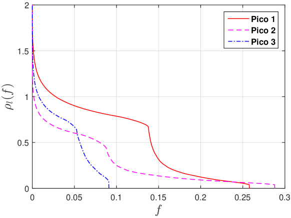
(a) $\rho_{l}(f)$ versus $f$.

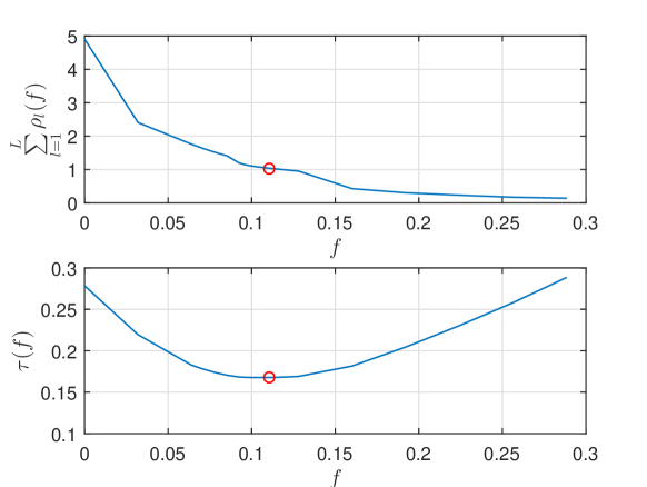
(b) $\sum_{l=1}^{L}\rho_{l}(f)$ and $\tau(f)$ versus $f$.

Figure 2: Heterogeneous scenario. $W=1$ MHz and $C_{l}=200$, $l\in\mathcal{L}$.

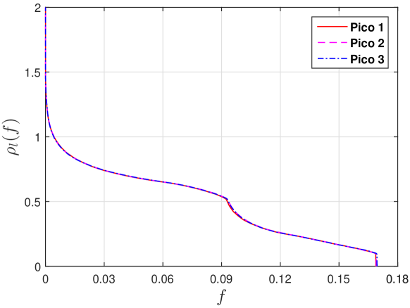
(a) $\rho_{l}(f)$ versus $f$.

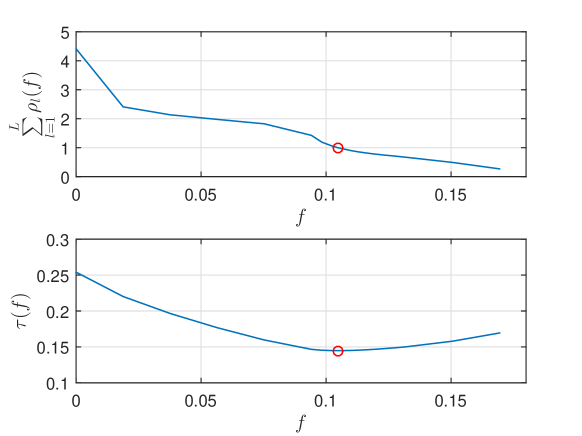
(b) $\sum_{l=1}^{L}\rho_{l}(f)$ and $\tau(f)$ versus $f$.

Figure 3: Homogenous scenario. $W=1$ MHz and $C_{l}=200$, $l\in\mathcal{L}$.

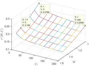
Figure 4: Minimum total time versus $W$ (MHz) and $C_{l}$ (files). $C_{l}$, $l\in\mathcal{L}$ are the same.

Appendix A: Proof of Lemma 1

We shall solve a relaxed version of Problem 3 where (3) is replaced with

$$s_{l,n}\in[0,1],\quad n\in\mathcal{N}.$$ (15)

We shall show that the optimal solution to the relaxed problem satisfies (3), and hence is also the optimal solution to Problem 3.

Let $\rho_{l}$ denote the Lagrangian multiplier w.r.t. (1). The corresponding Lagrangian is given by

$$\mathcal{L}(\{\mathbf{x}_{l}(\xi)\},\mathbf{s}_{l},\rho_{l})$$

$$= \sum_{n=1}^{N}\int_{\mathcal{K}_{l}}\frac{1-x_{l,n}(\xi)}{WR_{0}(\xi)}p_{n}\lambda(d\xi)$$

$$+\sum_{n=1}^{N}\int_{\mathcal{K}_{l}}\frac{(1-s_{l,n})x_{l,n}(\xi)}{WB_{l}}p_{n}\lambda(d\xi)$$

$$+\rho_{l}\left(\sum_{n=1}^{N}\int_{\mathcal{K}_{l}}\frac{x_{l,n}(\xi)}{WR_{l}(\xi)}p_{n}\lambda(d\xi)-f\right)$$

$$= \sum_{n=1}^{N}\int_{\mathcal{K}_{l}}\left(\frac{\rho_{l}}{WR_{l}(\xi)}+\frac{1-s_{l,n}}{WB_{l}}-\frac{1}{WR_{0}(\xi)}\right)x_{l,n}(\xi)p_{n}\lambda(d\xi)$$

$$+\sum_{n=1}^{N}\int_{\mathcal{K}_{l}}\frac{1}{WR_{0}(\xi)}p_{n}\lambda(d\xi)-\rho_{l}f$$

where $\{\mathbf{x}_{l}(\xi)\}$ and $\mathbf{s}_{l}$ satisfy (2), (15), and (4). Minimizing the Lagrangian w.r.t. $\{\mathbf{x}_{l}(\xi)\}$ subject to (2), we have

$$x_{l,n}(\xi,s_{l,n},\rho_{l})= \begin{cases}1,&\rho_{l}(\xi,s_{l,n})>\rho_{l}\\ 0,&\text{otherwise}\end{cases}$$ (16)

and

$$\min_{\{\mathbf{x}_{l}(\xi):\eqref{eqn:x-constr}\}}\mathcal{L}(\{\mathbf{x}_{l}(\xi)\},\mathbf{s}_{l},\rho_{l})$$

$$= \sum_{n=1}^{N}p_{n}\int_{\mathcal{A}_{l}(\rho_{l},s_{l,n})}\left(\frac{\rho_{l}}{WR_{l}(\xi)}+\frac{1-s_{l,n}}{WB_{l}}-\frac{1}{WR_{0}(\xi)}\right)\lambda(d\xi)$$

$$+\sum_{n=1}^{N}\int_{\mathcal{K}_{l}}\frac{1}{WR_{0}(\xi)}p_{n}\lambda(d\xi)-\rho_{l}f.$$ (17)

Denote $a(s)\triangleq\int_{\mathcal{A}_{l}(\rho_{l},s)}\left(\frac{\rho_{l}}{WR_{l}(\xi)}+\frac{1-s}{WB_{l}}-\frac{1}{WR_{0}(\xi)}\right)\lambda(d\xi)$. Now we show that $a(s)$ is decreasing in $s$. Suppose $s>s^{\prime}\geq 0$. Then, we have $\mathcal{A}_{l}(\rho_{l},s^{\prime})\subset\mathcal{A}_{l}(\rho_{l},s)$, implying $\mathcal{A}_{l}(\rho_{l},s)-\mathcal{A}_{l}(\rho_{l},s^{\prime})\subset\mathcal{A}_{l}(\rho_{l},s)$. Thus, we have

$$a(s)-a(s^{\prime})$$

$$= \int_{\mathcal{A}_{l}(\rho_{l},s)-\mathcal{A}_{l}(\rho_{l},s^{\prime})}\left(\frac{\rho_{l}}{WR_{l}(\xi)}+\frac{1-s}{WB_{l}}-\frac{1}{WR_{0}(\xi)}\right)\lambda(d\xi)$$

$$-\int_{\mathcal{A}_{l}(\rho_{l},s^{\prime})}\left(\frac{s-s^{\prime}}{WB_{l}}\right)\lambda(d\xi)<0$$

as $\frac{\rho_{l}}{WR_{l}(\xi)}+\frac{1-s}{WB_{l}}-\frac{1}{WR_{0}(\xi)}<0$ for $\xi\in\mathcal{A}_{l}(\rho_{l},s)$ and $s-s^{\prime}>0$. In addition, since $p_{n}$ is decreasing in $n$, further minimizing (17) w.r.t. $\mathbf{s}_{l}$ subject to (15) and (4), we can obtain (5) and the dual function

$$g_{l}(\rho_{l},f)$$

$$= \min_{\{\mathbf{x}_{l}(\xi):\eqref{eqn:x-constr}\},\{\mathbf{s}_{l}:\eqref{eqn:s-constr-cont},\eqref{eqn:cache-constr}\}}\mathcal{L}(\{\mathbf{x}_{l}(\xi)\},\mathbf{s}_{l},\rho_{l})$$

$$= \sum_{n=1}^{C_{l}}\int_{\mathcal{A}_{l}(\rho_{l},1)}\left(\frac{\rho_{l}}{WR_{l}(\xi)}-\frac{1}{WR_{0}(\xi)}\right)p_{n}\lambda(d\xi)$$

$$+\sum_{n=C_{l}+1}^{N}\int_{\mathcal{A}_{l}(\rho_{l},0)}\left(\frac{\rho_{l}}{WR_{l}(\xi)}+\frac{1}{WB_{l}}-\frac{1}{WR_{0}(\xi)}\right)p_{n}\lambda(d\xi)$$

$$+\sum_{n=1}^{N}\int_{\mathcal{K}_{l}}\frac{1}{WR_{0}(\xi)}p_{n}\lambda(d\xi)-\rho_{l}f$$ (18)

which is convex in $\rho_{l}$. On differentiating w.r.t. $\rho_{l}$ under the integral sign, we have

$$g_{l}^{\prime}(\rho_{l},f)= \sum_{n=1}^{C_{l}}\int_{\mathcal{A}_{l}(\rho_{l},1)}\frac{1}{WR_{l}(\xi)}p_{n}\lambda(d\xi)$$

$$+\sum_{n=C_{l}+1}^{N}\int_{\mathcal{A}_{l}(\rho_{l},0)}\frac{1}{WR_{l}(\xi)}p_{n}\lambda(d\xi)-f$$ (19)

which is continuous in $\rho_{l}$. Note that $g_{l}^{\prime}(\rho_{l},f)\in[-f,\bar{f_{l}}-f]$. The dual problem is given by

$$\tau_{l}(f)=\max_{\rho_{l}\geq 0}g_{l}(\rho_{l},f).$$ (20)

Since the dual problem is convex, when $f\leq\bar{f_{l}}$, the optimal dual variable satisfies $g_{l}^{\prime}(\rho_{l},f)=0$. When $f>\bar{f_{l}}$, $g_{l}^{\prime}(\rho_{l},f)<0$, the optimal dual variable is 0. Thus, the optimal dual value is given by

$$\tau_{l}(f)= \int_{\mathcal{K}_{l}}\frac{1}{WR_{0}(\xi)}\lambda(d\xi)-S_{C_{l}}\int_{\mathcal{A}_{l}(\rho_{l}(f),1)}\frac{1}{WR_{0}(\xi)}\lambda(d\xi)$$

$$-(1-S_{C_{l}})\int_{\mathcal{A}_{l}(\rho_{l}(f),0)}\left(\frac{1}{WR_{0}(\xi)}-\frac{1}{WB_{l}}\right)\lambda(d\xi)$$

which is equal to (8). The corresponding $\{\mathbf{x}_{l}^{*}(\xi)\}$ given by (6) (with $\mathbf{s}_{l}$ given by (5)) is feasible. Therefore, by the Lagrange Sufficiency Theorem, (6) and (5) are the optimal solution to the relaxed version of Problem 3 for any given $f\geq 0$. Note that $\mathbf{s}_{l}^{*}$ given by (5) satisfies (3). Thus,(6) and (5) are also the optimal solution to Problem 3 for any given $f\geq 0$. As $x_{l,n}^{*}(\xi)$ is a function of $f$, we also write it as $x_{l,n}^{*}(\xi,f)$.

Appendix B: Proof of Lemma 2

Given $f\in(0,\bar{f_{l}})$, for suitable $\delta f>0$, we have

$$\tau_{l}(f)-\tau_{l}(f-\delta f)$$

$$= -S_{C_{l}}\int_{\begin{subarray}{c}\mathcal{A}_{l}(\rho_{l}(f),1)\\ -\mathcal{A}_{l}(\rho_{l}(f-\delta f),1)\end{subarray}}\frac{1}{WR_{0}(\xi)}\lambda(d\xi)$$

$$-(1-S_{C_{l}})\int_{\begin{subarray}{c}\mathcal{A}_{l}(\rho_{l}(f),0)\\ -\mathcal{A}_{l}(\rho_{l}(f-\delta f),0)\end{subarray}}\left(\frac{1}{WR_{0}(\xi)}-\frac{1}{WB_{l}}\right)\lambda(d\xi)$$

$$= -S_{C_{l}}\int_{\{\xi\in\mathcal{K}_{l}:\rho(\xi,1)\in[\rho_{l}(f),\rho_{l}(f-\delta f)]\}}\frac{\rho(\xi,1)}{WR_{l}(\xi)}\lambda(d\xi)$$

$$-(1-S_{C_{l}})\int_{\{\xi\in\mathcal{K}_{l}:\rho(\xi,0)\in[\rho_{l}(f),\rho_{l}(f-\delta f)]\}}\frac{\rho(\xi,0)}{WR_{l}(\xi)}\lambda(d\xi)$$

$$\stackrel{{\scriptstyle(a)}}{{=}} -\tilde{\rho_{l}}S_{C_{l}}\int_{\{\xi\in\mathcal{K}_{l}:\rho(\xi,1)\in[\rho_{l}(f),\rho_{l}(f-\delta f)]\}}\frac{1}{WR_{l}(\xi)}\lambda(d\xi)$$

$$-\hat{\rho_{l}}(1-S_{C_{l}})\int_{\{\xi\in\mathcal{K}_{l}:\rho(\xi,0)\in[\rho_{l}(f),\rho_{l}(f-\delta f)]\}}\frac{1}{WR_{l}(\xi)}\lambda(d\xi)$$

$$= -\tilde{\rho_{l}}S_{C_{l}}\Bigg{(}\int_{\mathcal{A}_{l}(\rho_{l}(f),1)}\frac{1}{WR_{l}(\xi)}\lambda(d\xi)$$

$$\hskip 42.67912pt-\int_{\mathcal{A}_{l}(\rho_{l}(f-\delta f),1)}\frac{1}{WR_{l}(\xi)}\lambda(d\xi)\Bigg{)}$$

$$-\tilde{\rho_{l}}(1-S_{C_{l}})\Bigg{(}\int_{\mathcal{A}_{l}(\rho_{l}(f),0)}\frac{1}{WR_{l}(\xi)}\lambda(d\xi)$$

$$\hskip 62.59605pt-\int_{\mathcal{A}_{l}(\rho_{l}(f-\delta f),0)}\frac{1}{WR_{l}(\xi)}\lambda(d\xi)\Bigg{)}+\Delta(\delta f)$$

$$= -\tilde{\rho_{l}}\Bigg{(}S_{C_{l}}\int_{\mathcal{A}_{l}(\rho_{l}(f),1)}\frac{1}{WR_{l}(\xi)}\lambda(d\xi)$$

$$\hskip 28.45274pt+(1-S_{C_{l}})\int_{\mathcal{A}_{l}(\rho_{l}(f),0)}\frac{1}{WR_{l}(\xi)}\lambda(d\xi)\Bigg{)}$$

$$+\tilde{\rho_{l}}\Bigg{(}S_{C_{l}}\int_{\mathcal{A}_{l}(\rho_{l}(f-\delta f),1)}\frac{1}{WR_{l}(\xi)}\lambda(d\xi)$$

$$\hskip 28.45274pt+(1-S_{C_{l}})\int_{\mathcal{A}_{l}(\rho_{l}(f-\delta f),0)}\frac{1}{WR_{0}(\xi)}\lambda(d\xi)\Bigg{)}+\Delta(\delta f)$$

$$= -\tilde{\rho_{l}}f+\tilde{\rho_{l}}(f-\delta f)+\Delta(\delta f)=-\tilde{\rho_{l}}\delta f+\Delta(\delta f)$$ (21)

where (a) is due to mean value theorem and $\tilde{\rho_{l}},\hat{\rho_{l}}\in[\rho_{l}(f),\rho_{l}(f-\delta f)]$, and $\Delta(\delta f)$ is defined as

$$\Delta(\delta f)$$

$$\triangleq (\tilde{\rho_{l}}-\hat{\rho_{l}})(1-S_{C_{l}})\int_{\mathcal{A}_{l}(\rho_{l}(f),0)-\mathcal{A}_{l}(\rho_{l}(f-\delta f),0)}\frac{1}{WR_{l}(\xi)}\lambda(d\xi)$$ (22)

Since $\tilde{\rho_{l}},\hat{\rho_{l}}\in[\rho_{l}(f),\rho_{l}(f-\delta f)]$, we have $|\tilde{\rho_{l}}-\hat{\rho_{l}}|\leq\rho_{l}(f-\delta f)-\rho_{l}(f)$. As $\rho_{l}(f)$ has a finite unique derivative for almost all $f$, we have $\rho_{l}(f-\delta f)-\rho_{l}(f)\leq C\delta f$ for some finite positive $C$. Thus, we can show $\Delta(\delta f)/\delta f\to 0$ as $\delta f\to 0$. Dividing $\delta f$ on both sides of (21) and taking $\delta f\to 0$, we can show $\tau_{l}^{\prime}(f)=-\rho_{l}(f)$ for all $f\in(0,\bar{f}_{l})$. On the other hand, when $f\in(f_{l},\bar{f})$, we have $\tau_{l}^{\prime}(f)=0$ by Corollary 1 and $\rho_{l}(f)=0$ by Lemma 1. Thus, when $f\in(f_{l},\bar{f})$, we can show $\tau_{l}^{\prime}(f)=-\rho_{l}(f)$. Therefore, we have $\tau^{\prime}(f)=1-\sum_{l=1}^{L}\rho_{l}(f)$ for all $f\in(0,\bar{f})$. If $\sum_{l=1}^{L}\bar{\rho_{l}}\leq 1$, then $\sum_{l=1}^{L}\rho_{l}(f)<1$ for all $f\in[0,\bar{f}]$, as $\sum_{l=1}^{L}\rho_{l}(f)<\sum_{l=1}^{L}\bar{\rho_{l}}$ for all $f\in(0,\underline{f})$. Thus, if $\sum_{l=1}^{L}\bar{\rho_{l}}\leq 1$, we have $\tau^{\prime}(f)>0$ for all $f\in(0,\bar{f})$, implying $f^{*}=0$. If $\sum_{l=1}^{L}\rho_{l}(\bar{f})\geq 1$, then $\sum_{l=1}^{L}\rho_{l}(f)\geq 1$ for all $f\in(0,\bar{f})$, as $\rho_{l}(f)$ is non-increasing in $f$. Thus, if $\sum_{l=1}^{L}\rho_{l}(\bar{f})\geq 1$, we have $\tau^{\prime}(f)<0$ for all $f\in(0,\bar{f})$, implying $f^{*}=\bar{f}$. Otherwise, $f^{*}\in(0,\bar{f})$. As $\tau(f)$ is convex in $f$, we know that $\tau^{\prime}(f^{*})=0$.

Appendix C: Proof of Lemma 3

Note that $\rho_{l}(f,W,S_{C_{l}})$ increases in $S_{C_{l}}$ and decreases in $W$. First, we show (11).

$$\tau_{l}(S_{C_{l}},W+\delta W,f)-\tau_{l}(S_{C_{l}},W,f)$$

$$= \int_{\mathcal{K}_{l}}\frac{1}{(W+\delta W)R_{0}(\xi)}\lambda(d\xi)$$

$$-S_{C_{l}}\int_{\mathcal{A}_{l}(\rho_{l}(S_{C_{l}},W+\delta W,f),1)}\frac{1}{(W+\delta W)R_{0}(\xi)}\lambda(d\xi)$$

$$-(1-S_{C_{l}})\int_{\mathcal{A}_{l}(\rho_{l}(S_{C_{l}},W+\delta W,f),0)}\Bigg{(}\frac{1}{(W+\delta W)R_{0}(\xi)}$$

$$\hskip 156.49014pt-\frac{1}{(W+\delta W)B_{l}}\Bigg{)}\lambda(d\xi)$$

$$-\int_{\mathcal{K}_{l}}\frac{1}{WR_{0}(\xi)}\lambda(d\xi)+S_{C_{l}}\int_{\mathcal{A}_{l}(\rho_{l}(S_{C_{l}},W,f),1)}\frac{1}{WR_{0}(\xi)}\lambda(d\xi)$$

$$+(1-S_{C_{l}})\int_{\mathcal{A}_{l}(\rho_{l}(S_{C_{l}},W,f),0)}\left(\frac{1}{WR_{0}(\xi)}-\frac{1}{WB_{l}}\right)\lambda(d\xi)$$

$$= -\frac{\delta W}{W}\int_{\mathcal{K}_{l}}\frac{1}{(W+\delta W)R_{0}(\xi)}\lambda(d\xi)$$

$$+\frac{\delta W}{W}S_{C_{l}}\int_{\mathcal{A}_{l}(\rho_{l}(S_{C_{l}},W+\delta W,f),1)}\frac{1}{(W+\delta W)R_{0}(\xi)}\lambda(d\xi)$$

$$+\frac{\delta W}{W}(1-S_{C_{l}})\int_{\mathcal{A}_{l}(\rho_{l}(S_{C_{l}},W+\delta W,f),0)}\Bigg{(}\frac{1}{(W+\delta W)R_{0}(\xi)}$$

$$\hskip 156.49014pt-\frac{1}{(W+\delta W)B_{l}}\Bigg{)}\lambda(d\xi)$$

$$-S_{C_{l}}\int_{\begin{subarray}{c}\mathcal{A}_{l}(\rho_{l}(S_{C_{l}},W+\delta W,f),1)\\ -\mathcal{A}_{l}(\rho_{l}(S_{C_{l}},W,f),1)\end{subarray}}\frac{1}{WR_{0}(\xi)}\lambda(d\xi)$$

$$-(1-S_{C_{l}})\int_{\begin{subarray}{c}\mathcal{A}_{l}(\rho_{l}(S_{C_{l}},W+\delta W,f),0)\\ -\mathcal{A}_{l}(\rho_{l}(S_{C_{l}},W,f),0)\end{subarray}}\left(\frac{1}{WR_{0}(\xi)}-\frac{1}{WB_{l}}\right)\lambda(d\xi)$$

$$\stackrel{{\scriptstyle(a)}}{{=}} -\frac{\delta W}{W}\tau_{l}(S_{C_{l}},W+\delta W,f)$$

$$-S_{C_{l}}\tilde{\rho_{l}}\int_{\begin{subarray}{c}\mathcal{A}_{l}(\rho_{l}(S_{C_{l}},W+\delta W,f),1)\\ -\mathcal{A}_{l}(\rho_{l}(S_{C_{l}},W,f),1)\end{subarray}}\frac{1}{WR_{l}(\xi)}\lambda(d\xi)$$

$$-(1-S_{C_{l}})\hat{\rho_{l}}\int_{\begin{subarray}{c}\mathcal{A}_{l}(\rho_{l}(S_{C_{l}},W+\delta W,f),0)\\ -\mathcal{A}_{l}(\rho_{l}(S_{C_{l}},W,f),0)\end{subarray}}\frac{1}{WR_{l}(\xi)}\lambda(d\xi)$$

$$= -\frac{\delta W}{W}\tau_{l}(S_{C_{l}},W+\delta W,f)-\tilde{\rho_{l}}(f-f)-\frac{\delta W}{W}\tilde{\rho_{l}}f$$

$$-\Delta(\delta W)$$ (23)

where (a) is due to mean value theorem and $\tilde{\rho_{l}},\hat{\rho_{l}}\in[\rho_{l}(S_{C_{l}},W+\delta W,f),\rho_{l}(S_{C_{l}},W,f)]$, and $\Delta(\delta f)$ is defined as

$$\Delta(\delta W)$$

$$\triangleq (1-S_{C_{l}})(\hat{\rho_{l}}-\tilde{\rho_{l}})\int_{\begin{subarray}{c}\mathcal{A}_{l}(\rho_{l}(S_{C_{l}},W+\delta W,f),0)\\ -\mathcal{A}_{l}(\rho_{l}(S_{C_{l}},W,f),0)\end{subarray}}\frac{1}{WR_{l}(\xi)}\lambda(d\xi)$$

Similarly, we can show $\Delta(\delta W)/\delta W\to 0$ as $\delta W\to 0$. Dividing $\delta W$ on both sides of (23) and taking $\delta W\to 0$, we can show (11).

Next, we show (12).

$$\tau_{l}(S_{C_{l}}+\delta S_{C_{l}},W,f)-\tau_{l}(f,W,S_{C_{l}})$$

$$= -(S_{C_{l}}+\delta S_{C_{l}})\int_{\mathcal{A}_{l}(\rho_{l}(S_{C_{l}}+\delta S_{C_{l}},W,f),1)}\frac{1}{WR_{0}(\xi)}\lambda(d\xi)$$

$$-(1-S_{C_{l}}-\delta S_{C_{l}})\int_{\mathcal{A}_{l}(\rho_{l}(S_{C_{l}}+\delta S_{C_{l}},W,f),0)}\left(\frac{1}{WR_{0}(\xi)}-\frac{1}{WB_{l}}\right)\lambda(d\xi)$$

$$+S_{C_{l}}\int_{\mathcal{A}_{l}(\rho_{l}(f,W,S_{C_{l}}),1)}\frac{1}{WR_{0}(\xi)}\lambda(d\xi)$$

$$+(1-S_{C_{l}})\int_{\mathcal{A}_{l}(\rho_{l}(f,W,S_{C_{l}}),0)}\left(\frac{1}{WR_{0}(\xi)}-\frac{1}{WB_{l}}\right)\lambda(d\xi)$$

$$= S_{C_{l}}\int_{\begin{subarray}{c}\mathcal{A}_{l}(\rho_{l}(f,W,S_{C_{l}}),1)\\ -\mathcal{A}_{l}(\rho_{l}(S_{C_{l}}+\delta S_{C_{l}},W,f),1)\end{subarray}}\frac{1}{WR_{0}(\xi)}\lambda(d\xi)$$

$$+(1-S_{C_{l}})\int_{\begin{subarray}{c}\mathcal{A}_{l}(\rho_{l}(f,W,S_{C_{l}}),0)\\ -\mathcal{A}_{l}(\rho_{l}(S_{C_{l}}+\delta S_{C_{l}},W,f),0)\end{subarray}}\left(\frac{1}{WR_{0}(\xi)}-\frac{1}{WB_{l}}\right)\lambda(d\xi)$$

$$-\delta S_{C_{l}}\Bigg{(}\int_{\mathcal{A}_{l}(\rho_{l}(S_{C_{l}}+\delta S_{C_{l}},W,f),1)}\frac{1}{WR_{0}(\xi)}\lambda(d\xi)$$

$$\hskip 14.22636pt-\int_{\mathcal{A}_{l}(\rho_{l}(S_{C_{l}}+\delta S_{C_{l}},W,f),0)}\left(\frac{1}{WR_{0}(\xi)}-\frac{1}{WB_{l}}\Bigg{)}\lambda(d\xi)\right)$$

$$\stackrel{{\scriptstyle(a)}}{{=}} \tilde{\rho_{l}}S_{C_{l}}\int_{\begin{subarray}{c}\mathcal{A}_{l}(\rho_{l}(f,W,S_{C_{l}}),1)\\ -\mathcal{A}_{l}(\rho_{l}(S_{C_{l}}+\delta S_{C_{l}},W,f),1)\end{subarray}}\frac{1}{WR_{l}(\xi)}\lambda(d\xi)$$

$$+\hat{\rho_{l}}(1-S_{C_{l}})\int_{\begin{subarray}{c}\mathcal{A}_{l}(\rho_{l}(f,W,S_{C_{l}}),0)\\ -\mathcal{A}_{l}(\rho_{l}(S_{C_{l}}+\delta S_{C_{l}},W,f),0)\end{subarray}}\frac{1}{WR_{l}(\xi)}\lambda(d\xi)$$

$$-\delta S_{C_{l}}\Bigg{(}\int_{\mathcal{A}_{l}(\rho_{l}(S_{C_{l}}+\delta S_{C_{l}},W,f),1)}\frac{1}{WR_{0}(\xi)}\lambda(d\xi)$$

$$-\int_{\mathcal{A}_{l}(\rho_{l}(S_{C_{l}}+\delta S_{C_{l}},W,f),0)}\left(\frac{1}{WR_{0}(\xi)}-\frac{1}{WB_{l}}\Bigg{)}\lambda(d\xi)\right)$$

$$= \tilde{\rho_{l}}S_{C_{l}}\int_{\mathcal{A}_{l}(\rho_{l}(f,W,S_{C_{l}}),1)}\frac{1}{WR_{l}(\xi)}\lambda(d\xi)$$

$$-\tilde{\rho_{l}}(S_{C_{l}}+\delta S_{C_{l}})\int_{\mathcal{A}_{l}(\rho_{l}(S_{C_{l}}+\delta S_{C_{l}},W,f),1)}\frac{1}{WR_{l}(\xi)}\lambda(d\xi)$$

$$+\hat{\rho_{l}}(1-S_{C_{l}})\int_{\mathcal{A}_{l}(\rho_{l}(f,W,S_{C_{l}}),0)}\frac{1}{WR_{l}(\xi)}\lambda(d\xi)$$

$$-\hat{\rho_{l}}(1-S_{C_{l}}-\delta S_{S_{C_{l}}})\int_{\mathcal{A}_{l}(\rho_{l}(S_{C_{l}}+\delta S_{C_{l}},W,f),0)}\frac{1}{WR_{l}(\xi)}\lambda(d\xi)$$

$$+\Delta_{1}(\delta S_{C_{l}})$$

$$= \tilde{\rho_{l}}(f-f)+\Delta_{1}(\delta S_{C_{l}})+\Delta_{2}(\delta S_{C_{l}})$$

$$= \Delta_{1}(\delta S_{C_{l}})+\Delta_{2}(\delta S_{C_{l}})$$

where (a) is due to mean value theorem and $\tilde{\rho_{l}},\hat{\rho_{l}}\in[\rho_{l}(f,W,S_{C_{l}}),\rho_{l}(S_{C_{l}}+\delta S_{C_{l}},W,f)]$, and $\Delta_{1}(\delta S_{C_{l}})$ and $\Delta_{2}(\delta S_{C_{l}})$ are defined as

$$\Delta_{1}(\delta S_{C_{l}})$$

$$\triangleq \tilde{\rho_{l}}\delta S_{C_{l}}\int_{\mathcal{A}_{l}(\rho_{l}(S_{C_{l}}+\delta S_{C_{l}},W,f),1)}\frac{1}{WR_{l}(\xi)}\lambda(d\xi)$$

$$-\hat{\rho_{l}}\delta S_{S_{C_{l}}}\int_{\mathcal{A}_{l}(\rho_{l}(S_{C_{l}}+\delta S_{C_{l}},W,f),0)}\frac{1}{WR_{l}(\xi)}\lambda(d\xi)$$

$$-\delta S_{C_{l}}\Bigg{(}\int_{\mathcal{A}_{l}(\rho_{l}(S_{C_{l}}+\delta S_{C_{l}},W,f),1)}\frac{1}{WR_{0}(\xi)}\lambda(d\xi)$$

$$-\int_{\mathcal{A}_{l}(\rho_{l}(S_{C_{l}}+\delta S_{C_{l}},W,f),0)}\left(\frac{1}{WR_{0}(\xi)}-\frac{1}{WB_{l}}\right)\lambda(d\xi)\Bigg{)}$$

$$\Delta_{2}(\delta S_{C_{l}})$$

$$\triangleq (\hat{\rho_{l}}-\tilde{\rho_{l}})(1-S_{C_{l}})\int_{\begin{subarray}{c}\mathcal{A}_{l}(\rho_{l}(f,W,S_{C_{l}}),0)\\ -\mathcal{A}_{l}(\rho_{l}(S_{C_{l}}+\delta S_{C_{l}},W,f),0)\end{subarray}}\frac{1}{WR_{l}(\xi)}\lambda(d\xi)$$

$$+(\hat{\rho_{l}}-\tilde{\rho_{l}})\delta S_{S_{C_{l}}}\int_{\mathcal{A}_{l}(\rho_{l}(S_{C_{l}}+\delta S_{C_{l}},W,f),0)}\frac{1}{WR_{l}(\xi)}\lambda(d\xi)$$ (24)

Similarly, we can show $\Delta_{2}(\delta S_{C_{l}})/\delta S_{C_{l}}\to 0$ as $\delta S_{C_{l}}\to 0$. In addition, we have

$$\lim_{\delta S_{C_{l}}\to 0}\frac{\Delta_{1}(\delta S_{C_{l}})}{\delta S_{C_{l}}}$$

$$= \int_{\mathcal{A}_{l}(\rho_{l}(f,W,S_{C_{l}}),1)}\left(\frac{\rho_{l}(f,W,S_{C_{l}})}{WR_{l}(\xi)}-\frac{1}{WR_{0}(\xi)}\right)\lambda(d\xi)$$

$$-\int_{\mathcal{A}_{l}(\rho_{l}(f,W,S_{C_{l}}),0)}\left(\frac{\rho_{l}(f,W,S_{C_{l}})}{WR_{l}(\xi)}-\left(\frac{1}{WR_{0}(\xi)}-\frac{1}{WB_{l}}\right)\right)\lambda(d\xi)$$

$$= \int_{\begin{subarray}{c}\mathcal{A}_{l}(\rho_{l}(f,W,S_{C_{l}}),1)\\ -\mathcal{A}_{l}(\rho_{l}(f,W,S_{C_{l}}),0)\end{subarray}}\left(\frac{\rho_{l}(f,W,S_{C_{l}})}{WR_{l}(\xi)}-\frac{1}{WR_{0}(\xi)}\right)\lambda(d\xi)$$

$$-\int_{\mathcal{A}_{l}(\rho_{l}(f,W,S_{C_{l}}),0)}\frac{1}{WB_{l}}\lambda(d\xi)$$

$$< 0$$ (25)

Thus, we can show (12).

Appendix D: Proof of Theorem 2

By Lemma 3, we have $\tau(f,W,\mathbf{C})\leq\tau(f,W^{\prime},\mathbf{C}^{\prime})$. Thus, we have $\tau(f,W^{\prime},\mathbf{C}^{\prime})\geq\tau(f^{*}(W^{\prime},\mathbf{C}^{\prime}),W^{\prime},\mathbf{C}^{\prime})\geq\tau(f^{*}(W^{\prime},\mathbf{C}^{\prime}),W,\mathbf{C})\geq\tau(f^{*}(W,\mathbf{C}),W,\mathbf{C})$. Note that $\tau^{*}(W^{\prime},\mathbf{C}^{\prime})\triangleq\tau(f^{*}(W^{\prime},\mathbf{C}^{\prime}),W^{\prime},\mathbf{C}^{\prime})$ and $\tau^{*}(W,\mathbf{C})\triangleq\tau(f^{*}(W,\mathbf{C}),W,\mathbf{C})$. Therefore, we complete the proof.

References

- [1] A. Ghosh, N. Mangalvedhe, R. Ratasuk, B. Mondal, M. Cudak, E. Visotsky, T. Thomas, J. Andrews, P. Xia, H. Jo, H. Dhillon, and T. Novlan, “Heterogeneous cellular networks: From theory to practice,” IEEE Commun. Mag., vol. 50, no. 6, pp. 54–64, 2012.
- [2] K. Shanmugam, N. Golrezaei, A. Dimakis, A. Molisch, and G. Caire, “Femtocaching: Wireless content delivery through distributed caching helpers,” Information Theory, IEEE Transactions on, vol. 59, no. 12, pp. 8402–8413, Dec 2013.
- [3] K. Poularakis, G. Iosifidis, and L. Tassiulas, “Approximation algorithms for mobile data caching in small cell networks,” Communications, IEEE Transactions on, vol. 62, no. 10, pp. 3665–3677, Oct 2014.
- [4] E. Bastu, M. Bennis, M. Kountouris, and M. Debbah, “Cache-enabled small cell networks: Modeling and tradeoffs,” EURASIP Journal on Wireless Communications and Networking, 2015.
- [5] D. Liu and C. Yang, “Cache-enabled heterogeneous cellular networks: Comparison and tradeoffs,” in IEEE Int. Conf. on Commun. (ICC), Kuala Lumpur, Malaysia, June 2016.
- [6] C. Yang, Y. Yao, Z. Chen, and B. Xia, “Analysis on cache-enabled wireless heterogeneous networks,” Wireless Communications, IEEE Transactions on, vol. 15, no. 1, pp. 131–145, Jan 2016.
- [7] F. Pantisano, M. Bennis, W. Saad, and M. Debbah, “Cache-aware user association in backhaul-constrained small cell networks,” in Modeling and Optimization in Mobile, Ad Hoc, and Wireless Networks (WiOpt), 2014 12th International Symposium on, May 2014, pp. 37–42.
- [8] S. Hanly, C. Liu, and P. Whiting, “Capacity and stable scheduling in heterogeneous wireless networks,” Selected Areas in Communications, IEEE Journal on, vol. 33, no. 6, pp. 1266–1279, June 2015.