Non-perturbative renormalization of the axial current in $N_{\rm f}=3$ lattice QCD with Wilson fermions and tree-level improved gauge action

Abstract

We non-perturbatively determine the renormalization factor of the axial vector current in lattice QCD with $N_{\rm f}=3$ flavors of Wilson-clover fermions and the tree-level Symanzik-improved gauge action. The (by now standard) renormalization condition is derived from the massive axial Ward identity and it is imposed among Schrödinger functional states with large overlap on the lowest lying hadronic state in the pseudoscalar channel, in order to reduce kinematically enhanced cutoff effects. We explore a range of couplings relevant for simulations at lattice spacings of $\approx 0.09\,{\rm fm}$ and below. An interpolation formula for $Z_{\rm A}(g_{0}^{2})$, smoothly connecting the non-perturbative values to the 1-loop expression, is provided together with our final results.

1 Introduction

It is well known that chiral symmetry is explicitly broken in the Wilson lattice regularization of QCD [1]. As a consequence of that, the isovector axial current does not satisfy the continuum Ward-Takahashi identities. These can be restored up to cutoff effects by a finite renormalization of the axial vector current [2]. Previous computations by the ALPHA Collaboration in the quenched [3] and in the two-flavor dynamical cases [4, 5] have shown that at the lattice spacings $a$ typically simulated ($0.04\;{\rm fm}\;\lesssim a\lesssim\;0.1\;{\rm fm}$), this renormalization factor $Z_{\rm A}$ differs significantly from its (1-loop) perturbative estimate. Since it is required for the computation of pseudoscalar decay constants and thus, e.g., in the scale setting procedure (through $F_{\pi}$ or $F_{\rm K}$, as done in [6] for $N_{\rm f}=2$ and launched in [7] for $N_{\rm f}=2+1$), as well as in the computation of light [8, 6] and heavy [9, 10] quark masses, it is of paramount importance to determine $Z_{\rm A}$ non-perturbatively.

Here we report about a non-perturbative determination of $Z_{\rm A}$ in lattice QCD with $N_{\rm f}=3$ mass-degenerate flavors of Wilson-clover fermions and the tree-level Symanzik-improved gauge action [11]. For a calculation in the three-flavor theory with stout-smeared quarks and RG-improved Iwasaki gluon action, see Ref. [12].

The improvement coefficient $c_{\rm sw}$ of lattice QCD with $N_{\rm f}=3$ O$(a)$ improved Wilson fermions and tree-level Symanzik-improved gauge action has been non-perturbatively tuned in [13]. Our computation of $Z_{\rm A}$, a preliminary account of which was already given in [14], is performed with Schrödinger functional boundary conditions, and we use the same method adopted in [5] for the $N_{\rm f}=2$ case. In particular, the normalization condition exploits the full, massive axial Ward identity in order to reduce finite quark mass uncertainties in the evaluation of $Z_{\rm A}$. Correlators are built using optimized boundary wave-functions such that cutoff effects due to excited state contributions are suppressed. The setup in the present work concerning the simulation parameters and the choice of boundary interpolating fields (wave-functions) is the same as the one recently employed for the computation of the improvement coefficient $c_{\rm A}$ [15].

We discuss the relevant equations for the normalization condition in Section 2 and provide some simulation details in Section 3. Numerical results and the final interpolation formula are presented in Section 4, together with a discussion of residual systematic effects. Section 5 contains our summary.

2 Renormalization condition

The condition that we choose in order to normalize the axial current has been originally introduced for the case of two dynamical fermions in [4]. In this section we give a short account of its derivation. More details can be found in the quoted paper.

The Partially Conserved Axial Current (PCAC) relations are the set of (infinite) Ward identities derived performing a chiral rotation of the quark fields. By restricting the transformation to a region $R$, one can derive different operator relations depending on the particular choice of composite fields inserted internally and externally w.r.t. the region $R$. If the axial current $A_{\nu}^{b}(y)$ is chosen as internal operator, the resultant identities can be cast in the integrated form [16]

$$\int_{\partial R}\mathrm{d}{\sigma_{\mu}(x)}\;\left\langle A_{\mu}^{a}(x)A_{\nu}^{b}(y)\mathcal{O}_{\mathrm{ext}}\right\rangle-2m\int_{R}\mathrm{d}^{4}{x}\;\left\langle P^{a}(x)A_{\nu}^{b}(y)\mathcal{O}_{\mathrm{ext}}\right\rangle=i\epsilon^{abc}\left\langle V_{\nu}^{c}(y)\mathcal{O}_{\mathrm{ext}}\right\rangle,$$ (2.1)

where $a,\,b$ and $c$ are flavor indices in a SU(2) sub-group of the chiral group SU(3). In the equation above, $R$ (containing $y$) is still arbitrary and $\mathcal{O}_{\mathrm{ext}}$ is an operator built from fields outside $R$. $V_{\nu}^{c}$ is the isovector vector current. Further specifying $R$ as the spacetime volume between two space-like hyperplanes and setting $\nu=0$, after contracting the flavor indices $a$ and $b$ with $\epsilon^{abc}$, one arrives at

$$\int\mathrm{d}^{3}{{\bf x}}\;\mathrm{d}^{3}{{\bf y}}\;\epsilon^{abc}\left\langle A_{0}^{a}(x)\,A_{0}^{b}(y)\,\mathcal{O}_{\mathrm{ext}}\right\rangle\\ {}-2m\int\mathrm{d}^{3}{{\bf x}}\;\mathrm{d}^{3}{{\bf y}}\;\int_{y_{0}}^{x_{0}}\mathrm{d}{x_{0}}\;\epsilon^{abc}\left\langle P^{a}(x)\,A_{0}^{b}(y)\,\mathcal{O}_{\mathrm{ext}}\right\rangle\\ =i\int\mathrm{d}^{3}{{\bf y}}\;\left\langle V_{0}^{c}(y)\,\mathcal{O}_{\mathrm{ext}}\right\rangle$$ (2.2)

with $x_{0}>y_{0}$ defining the hyperplanes. It is clear that the above relation, once considered at the renormalized level, relates the normalization of the axial current to that of the vector current. A condition for the latter will be implicitly given below.

We evaluate the identity in eq. (2.2) on the lattice with Schrödinger functional boundary conditions (periodic in space, Dirichlet in time) [17, 18] with vanishing background field. The source operator $\mathcal{O}_{\mathrm{ext}}$ is expressed in terms of the quark fields $\zeta$ and $\zeta\kern 1.0pt^{\prime}$ at the boundaries $x_{0}=0$ and $x_{0}=T$ as

$$\mathcal{O}_{\mathrm{ext}}=-\frac{1}{6L^{6}}\epsilon^{cde}{\cal O}\kern-7.7778pt\kern 7.7778pt\smash{\raise 4.5pt\hbox{\kern 1.0pt$\scriptstyle\prime$}}\kern 1.0pt^{d}{\mathcal{O}}^{e}$$ (2.3)

with

$${\mathcal{O}}^{e}=a^{6}\sum_{{\bf u},{\bf v}}\overline{\zeta}({\bf u})\,\gamma_{5}\,\frac{\tau^{e}}{2}\,\omega({\bf u}-{\bf v})\,\zeta({\bf v})\;\;\text{and}\;\;{\cal O}\kern-7.7778pt\kern 7.7778pt\smash{\raise 4.5pt\hbox{\kern 1.0pt$\scriptstyle\prime$}}\kern 1.0pt^{d}=a^{6}\sum_{{\bf u},{\bf v}}\overline{\zeta}\kern 1.0pt^{\prime}({\bf u})\,\gamma_{5}\,\frac{\tau^{d}}{2}\,\omega({\bf u}-{\bf v})\,\zeta\kern 1.0pt^{\prime}({\bf v})\;.$$ (2.4)

The wave-function $\omega$ is optimized in order to excite states with a large projection on the pseudoscalar ground state. Its construction is detailed in [15]. The free index $c$ in eq. (2.3) is contracted with the free index in eq. (2.2). In this case, the term on the right-hand side involving the isospin charge density can be simplified to the boundary-to-boundary correlator

$$F_{1}=-\frac{1}{3L^{6}}\left\langle{\cal O}\kern-7.7778pt\kern 7.7778pt\smash{\raise 4.5pt\hbox{\kern 1.0pt$\scriptstyle\prime$}}\kern 1.0pt^{a}{\mathcal{O}}^{a}\right\rangle$$ (2.5)

up to ${\rm O}(a^{2})$, as it has been shown in [3, 4] by using isospin symmetry.

After replacing all terms by their improved and renormalized lattice counterparts, the Ward identity can be written as

$$Z_{\rm A}^{2}\left(1+b_{\rm A}\,am_{\rm q}\right)^{2}\left[F_{\mathrm{AA}}^{\rm I}(x_{0},y_{0})-2m\cdot\tilde{F}_{\mathrm{PA}}^{\rm I}(x_{0},y_{0})\right]=F_{1},$$ (2.6)

with the improved correlation functions

$$F_{\mathrm{AA}}^{\rm I}(x_{0},y_{0}) =F_{\mathrm{AA}}(x_{0},y_{0})+ac_{\rm A}\left[\tilde{\partial}_{x_{0}}F_{\mathrm{PA}}(x_{0},y_{0})+\tilde{\partial}_{y_{0}}F_{\mathrm{AP}}(x_{0},y_{0})\right]$$ (2.7)

$$\qquad+\,a^{2}c_{\rm A}^{2}\,\tilde{\partial}_{x_{0}}\tilde{\partial}_{y_{0}}F_{\mathrm{PP}}(x_{0},y_{0}),$$

$${\rm and}\quad\tilde{F}_{\mathrm{PA}}^{\rm I}(x_{0},y_{0}) =a\sum_{x^{\prime}_{0}=y_{0}}^{x_{0}}w(x^{\prime}_{0})\left[F_{\mathrm{PA}}(x_{0},y_{0})+ac_{\rm A}\,\partial_{y_{0}}F_{\mathrm{PP}}(x_{0},y_{0})\right],$$ (2.8)

where $\tilde{\partial}$ denotes the central difference operator and $F_{XY}(x_{0},y_{0})$ with $X,Y\in\{A_{0},P\}$ reads

$$F_{XY}(x_{0},y_{0})=-\frac{a^{6}}{6L^{6}}\sum_{{\bf x},{\bf y}}\epsilon^{abc}\epsilon^{cde}\left\langle{\cal O}\kern-7.7778pt\kern 7.7778pt\smash{\raise 4.5pt\hbox{\kern 1.0pt$\scriptstyle\prime$}}\kern 1.0pt^{d}X^{a}(x)Y^{b}(y){\mathcal{O}}^{e}\right\rangle\;,$$ (2.9)

and

$$w(x^{\prime}_{0})=\begin{cases}1/2&\text{if $x^{\prime}_{0}=y_{0}$ or $x^{\prime}_{0}=x_{0}$}\\ 1&\text{if $y_{0}<x^{\prime}_{0}<x_{0}$}\end{cases}$$ (2.10)

implements the trapezoidal rule. In eq. (2.6) the bare quark mass $m$ is defined through the PCAC relation, while $m_{\rm q}$ is the bare subtracted quark mass. The mass-dependent improvement term proportional to $b_{\rm A}$ will be neglected from here on, since we will impose the renormalization condition at vanishing mass. Any mistuning will result in ${\rm O}(am)$ effects, as effects of ${\rm O}(\Lambda_{\rm QCD}m)$ are explicitly removed by using the massive Ward identity. Our final renormalization condition thus reads

$$Z_{\rm A}=\lim_{m\to 0}\left[\frac{F_{1}}{F_{\mathrm{AA}}^{\rm I}(x_{0},y_{0})-2m\cdot\tilde{F}_{\mathrm{PA}}^{\rm I}(x_{0},y_{0})}\right]^{\frac{1}{2}}.$$ (2.11)

In order to maximize the distance between the insertion points and to keep this distance physical (once $L$ is fixed), we choose $x_{0}=\frac{2}{3}T$ and $y_{0}=\frac{1}{3}T$.

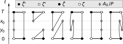
Figure 1: The six non-vanishing Wick contractions contributing to the correlation functions $F_{XY}$ with sources ${\mathcal{O}}^{\mathrm{ext}}$ on the boundaries and two insertions of the operators $X$ and $Y$ in the bulk, see eq. (2.9), taken from [4].

Except for $F_{1}$, only correlators of the form given in eq. (2.9) appear in eq. (2.11). After working out the Wick contractions, one finds that only six diagrams contribute to those. They are depicted in figure 1. Two of them are disconnected, and as showed in Appendix A of Ref. [4], they only give rise to ${\rm O}(a^{2})$ contributions and vanish in the massless continuum limit. By omitting them and taking only the connected contractions, one obtains an alternative renormalization condition. The corresponding renormalization factor is denoted by $Z_{\rm A}^{\mathrm{con}}$ in the following. Although our preferred definition remains the one including all quark-contractions, $Z_{\rm A}^{\mathrm{con}}$ offers the possibility to further check the smooth dependence of $Z_{\rm A}$ on the gauge coupling, as a consequence of the constant physics setup, as well as the smooth ${\rm O}(a^{2})$ convergence of different renormalization conditions from the explored non-perturbative region to the perturbative regime.

An alternative renormalization condition, using the Schrödinger functional with chirally rotated boundary conditions, has been recently proposed and tested in perturbation theory [19] and non-perturbatively in the quenched and in the $N_{\rm f}=2$ cases [20, 21]. The main advantage of the approach being that it entails automatic O($a$) improvement, it seems very promising and, in two-flavor QCD, turned out to yield more precise results than with standard Schrödinger functional boundary conditions [21].

3 Simulation details

The ensembles used in this study coincide with those considered in [15], and algorithmic details can be found there. In a few cases the number of configurations has actually been enlarged, and in addition we generated a new ensemble (at $L/a=14$) with the purpose of better constraining the final parameterization of the renormalization constant in the region where the dependence on the gauge coupling is strongest.

Our three-flavor lattice QCD simulations with Schrödinger functional boundary conditions used the openQCD codeof Ref. [22]. In order to ensure a smooth dependence of the renormalization constant $Z_{\rm A}$ on the bare gauge coupling, we have approximately fixed a constant physics condition by setting $L\approx 1.2\,\mathrm{fm}$. That is achieved by beginning with a particular pair of $g_{0}^{2}$ and $L/a$ ($\beta=6/g_{0}^{2}=3.3$ at $L/a=12$ here) and then choosing the bare couplings for subsequent smaller lattice spacings according to the universal 2-loop $\beta$-function. In this way we cover lattice spacings in the range from $a\approx 0.09\,{\rm fm}$ to $a\approx 0.045\,{\rm fm}$. At each bare coupling we have tuned the bare quark mass so that the PCAC mass is close to zero. We could check at several lattice spacings that our determination of $Z_{\rm A}$ is insensitive to variations of the (small) quark mass. Information about our ensembles, consisting in most cases of several replica per parameter set, are summarized in Tab. 1. For practical reasons discussed in the openQCD documentation, our lattices have temporal extents $T=3L/2-a$. Since we use an ${\rm O}(a)$ improved setup, this offset is expected to influence the determination of $Z_{\rm A}$ at ${\rm O}(a^{3})$ only.

$L^{3}\times T/a^{4}$			$\beta$		$\kappa$	# REP	# MDU		ID
$12^{3}\times 17$			3.3		0.13652	10	10240		A1k1
					0.13660	10	12620		A1k2
$14^{3}\times 21$			3.414		0.13690	32	10360		E1k1
					0.13695	48	13984		E1k2
$16^{3}\times 23$			3.512		0.13700	2	20480		B1k1
					0.13703	1	8192		B1k2
					0.13710	3	24560		B1k3
$16^{3}\times 23$			3.47		0.13700	3	29584		B2k1
$20^{3}\times 29$			3.676		0.13700	4	15232		C1k2
					0.13719	4	15472		C1k3
$24^{3}\times 35$			3.810		0.13712	5	10240		D1k1

Table 1: Summary of simulation parameters, number of replica and total number of molecular dynamics units of our gauge configuration ensembles labeled by ‘ID’, used for the determination of the renormalization factor $Z_{\rm A}$. Compared to the data basis underlying our earlier computation of $c_{\rm A}$ in [15], the analysis presented here includes the additional $L/a=14$ lattice ensembles {E1k1, E1k2}. Also note that the statistics of ensemble B2k1 have been increased by more than a factor of three.

In the context of our earlier computation of $c_{\rm A}$ [15], we already estimated the deviation from the, perturbatively implemented, constant $L$ condition, which is also imposed here, by measuring the scale-dependent renormalized coupling $\bar{g}_{\rm GF}^{2}$, defined in Ref. [23]. The results for this coupling apply here, too, and can be found in Tab. 2 of Ref. [15]. Finally, we also test the dependence of $Z_{\rm A}$ on $L$ in physical units directly by simulating an additional bare coupling at $L/a=16$.

4 Results

We measure the correlation functions defined in Section 2 on each fourth trajectory of length $\tau=2\,\mathrm{MDU}$ so that the spacing between the measurements is $8\,\mathrm{MDU}$. Only on the A1k2 ensemble, we use a measurement separation of $2\tau=4\,\mathrm{MDU}$. The total statistics for the different ensembles are given in Tab. 1.

For diagnostic purposes, we also compute ‘smoothed’ gauge field observables obtained from the Wilson (gradient) flow [24]. We fix the flow time $t$ by setting $\sqrt{8t}/L=c$ with $c=0.35$. The smoothed gauge fields provide a renormalized definition of the topological charge $Q$, which we use to monitor the topology freezing; in addition, even at lattice spacings where topology freezing does not occur, the smoothed topological charge and action typically possess the largest observed autocorrelation times. Finally, the coupling $\bar{g}_{\rm GF}^{2}$ of Ref. [23], defined through the Wilson flow, may be used to monitor the deviation from the constant physics condition, as it depends only on the physical lattice size up to cutoff effects. For results on this coupling we refer again to Tab. 2 in [15], where one can see that $\bar{g}_{\rm GF,0}^{2}(L)$ (i.e., the gradient flow coupling within the zero topology sector, see below) varies between 14 and 18 on our ensembles. That roughly corresponds to a 20% variation in $L$.

ID		$am_{\mathrm{PCAC}}$		$am_{{\mathrm{PCAC}},0}$		$Z_{\rm A}$		$Z_{\mathrm{A},0}$		$Z_{\mathrm{A}}^{\mathrm{con}}$		$Z_{\mathrm{A},0}^{\mathrm{con}}$
A1k1		$-0$.	$00234(85)$	$-0$.	$00367(92)$	$0$.	$641(13)$	$0$.	$636(16)$	$0$.	$809(11)$	$0$.	$811(12)$
A1k2		$-0$.	$01085(71)$	$-0$.	$01206(81)$	$0$.	$6432(98)$	$0$.	$638(11)$	$0$.	$833(11)$	$0$.	$835(16)$
		$0$.	$0$	$0$.	$0$	$0$.	$6424(78)$	${\it 0}$.	${\it 6374(91)}$	$0$.	$8210(78)$	$0$.	$8196(96)$
E1k1		$0$.	$00275(38)$	$0$.	$00262(49)$	$0$.	$7148(99)$	$0$.	$727(14)$	$0$.	$7705(91)$	$0$.	$7743(98)$
E1k2		$0$.	$00004(33)$	$-0$.	$00072(41)$	$0$.	$7151(93)$	$0$.	$702(13)$	$0$.	$7892(98)$	$0$.	$773(18)$
		$0$.	$0$	$0$.	$0$	$0$.	$7150(68)$	${\it 0}$.	${\it 7136(95)}$	$0$.	$7792(67)$	$0$.	$7740(86)$
B1k1		$0$.	$00565(16)$	$0$.	$00554(23)$	$0$.	$7666(47)$	$0$.	$7602(72)$	$0$.	$7743(24)$	$0$.	$7744(43)$
B1k2		$0$.	$00494(25)$	$0$.	$00423(36)$	$0$.	$7676(71)$	$0$.	$766(10)$	$0$.	$7759(44)$	$0$.	$7779(63)$
B1k3		$0$.	$00160(18)$	$0$.	$00109(21)$	$0$.	$7521(39)$	$0$.	$7515(52)$	$0$.	$7806(30)$	$0$.	$7757(41)$
		$0$.	$0$	$0$.	$0$	$0$.	$7595(28)$	${\it 0}$.	${\it 7562(39)}$	$0$.	$7766(17)$	$0$.	$7756(27)$
B2k1		$0$.	$00349(17)$	$0$.	$00306(23)$	$0$.	$7456(44)$	$0$.	$7434(59)$	$0$.	$7778(27)$	$0$.	$7793(35)$
C1k2		$0$.	$00618(14)$	$0$.	$00610(25)$	$0$.	$7875(92)$	$0$.	$789(17)$	$0$.	$7904(22)$	$0$.	$7840(40)$
C1k3		$-0$.	$00082(12)$	$-0$.	$00099(13)$	$0$.	$7771(29)$	$0$.	$7779(31)$	$0$.	$7833(27)$	$0$.	$7841(29)$
		$0$.	$0$	$0$.	$0$	$0$.	$7780(28)$	${\it 0}$.	${\it 7783(30)}$	$0$.	$7876(17)$	$0$.	$7841(23)$
D1k1		n.	q.	$-0$.	$002909(72)$	n.	q.	${\it 0}$.	${\it 7897(19)}$	n.	q.	$0$.	$8009(35)$

Table 2: Summary of results for $Z_{\rm A}$. The (unrenormalized) PCAC quark mass $am_{\mathrm{PCAC}}$ is computed from the correlation functions projected to the approximate ground state, using the non-perturbative result for $c_{\rm A}(g_{0}^{2})$ from [15] and averaging the local mass over the central four timeslices. Here, quantities with the explicit subscript label ‘0’ refer to results from the analysis restricted to the sector of vanishing topological charge, whereas in the text we loosely suppress the ‘0’. Numbers for ensemble D1k1 ($L/a=24$) are not quoted (‘n.q.’) for the case of including all charge sectors in the partition sum, because owing to an insufficient sampling of all the sectors by our simulations a reliable error estimation is not possible. For those ensembles, where simulations at several quark masses were performed, the renormalization constant has been extrapolated to the chiral limit ($am_{\mathrm{PCAC}},am_{{\mathrm{PCAC}},0}\to 0$) taking a weighted average (i.e., fitting to a constant). Results in italics enter into the final interpolation formula for $Z_{\rm A}(g_{0}^{2})$, eq. (4.12).

As discussed in [15], for all simulations and all observables, we find that integrated autocorrelation times are bounded by $\tau_{\mathrm{max}}\lesssim 200-250\,\mathrm{MDU}$, except for our $L/a=24$ simulations where the charge is frozen. Since we are practically unable to sufficiently sample all topological sectors at this finest lattice spacing, we everywhere define observables restricted to the trivial, i.e., $Q=0$ sector. Note that the same strategy was followed in our non-perturbative determination of $c_{\rm A}$ in [15]. As shown in Tab. 2, the projection to the $Q=0$ sector does not induce a noticeable difference in the final numbers for $Z_{\rm A}$, which is expected since the Ward identities, being operator relations, are valid in each topological sector.

Statistical errors are estimated by applying a full autocorrelation analysis according to Ref. [25].

For the wave-functions $\omega$ in eq. (2.4), we use the same approach adopted in [15] and solve for the two largest eigenvectors of the matrix $F_{1}(\omega_{i}^{\prime},\omega_{j})$. These normalized eigenvectors have a well-defined continuum limit along our line of constant physics in parameter space, as long as the wave-functions depend on physical scales only. Since we do not observe any significant lattice spacing dependence for them, we fix these eigenvectors to the values calculated on the B1k2 ensemble ($L/a=16$, $\beta=3.512$, $\kappa=0.13703$) and regard that as part of our choice of the renormalization condition. The effective masses of the correlation function $f_{\rm P}$, after taking the inner product with the eigenvectors in wave-function space, indicate clearly distinct signals, providing evidence that those effectively maximize the overlap with the ground and first excited states (see Fig. 2 in [15]). Notice that, as opposed to the case of the computation of the improvement coefficient $c_{\rm A}$, here we only need the wave-function projecting onto the ground state.

In the following, we restrict the discussion of systematic effects to observables projected to the sector of vanishing topological charge: $am_{\mathrm{PCAC}}\equiv am_{{\mathrm{PCAC}},0}$, $Z_{\rm A}\equiv Z_{\rm A,0}$. As mentioned above, those are the ones entering our final results. In any case, the ‘un-projected’ quantities, where they can be properly estimated, display the same qualitative features.

As expected from the discussion in Section 2, for the massive normalization condition the data exhibit very little dependence on the quark mass, which implies that uncertainties due to the position of the critical mass do not affect the determination of $Z_{\rm A}$. We illustrate the chiral extrapolation $am_{\rm PCAC}\to 0$ at $\beta=3.512$ in Fig. 2. For this normalization condition, the slope in $am_{\rm PCAC}$ is consistent with zero, whereas the estimate of $Z_{\rm A}$ from the massless Ward identity (i.e., by setting directly $m=0$ in eq. (2.11)) changes by 25% in the very small mass range displayed. At all the other gauge couplings the situation is very similar, with $Z_{\rm A}$ from the massive Ward identity definition being mass-independent within errors, as evinced by Tab. 2. In fact, performing fits to a constant over the considered mass range yields suitably small $\chi^{2}$- and very reasonable goodness-of-fit-values and, therefore, is fully consistent with our data. Moreover, the slopes, which would come out of linear fits, are compatible with zero within one standard deviation for most ensembles (and within $1.5\sigma$ for all), and their magnitude is such that we do not expect them to have any relevant impact on our final results and errors. All this serves as a further justification of this chiral extrapolation procedure.

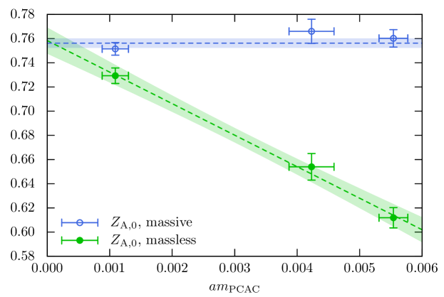
Figure 2: Chiral extrapolations for $Z_{\rm A}=Z_{\rm A,0}$ imposing the massive and massless conditions on ensembles {B1k1, B1k2, B1k3} at $L/a=16,\,\beta=3.512$. The data in the massive case, for which a slope is found to be statistically insignificant, are fitted to a constant.

Near the continuum, and in the ${\rm O}(a)$ improved theory, the dependence of renormalization factors on the lattice extent is expected to be an ${\rm O}\left((a/L)^{2}\right)$ effect, hence deviations from the line of constant physics should affect our determination of $Z_{\rm A}$ by the same amount. The B2k1 ensemble has been generated exactly with the purpose of checking these effects, as it differs from the ensembles in the B1 series by a 6% change in $L$. The value of $Z_{\rm A}$ determined there lies within one standard deviation from the chirally extrapolated value for the B1 series, and we are therefore confident that (small) variations of $L$ do not produce significant shifts in our estimates of $Z_{\rm A}$.

Our final results for $Z_{\rm A}$, after chiral extrapolations via performing fits to a constant at each $\beta$ as explained before, are shown in Fig. 3 as a function of $g_{0}^{2}$. One can see that the data lie on a smooth curve, which we describe by performing a Padé fit, producing the expression:

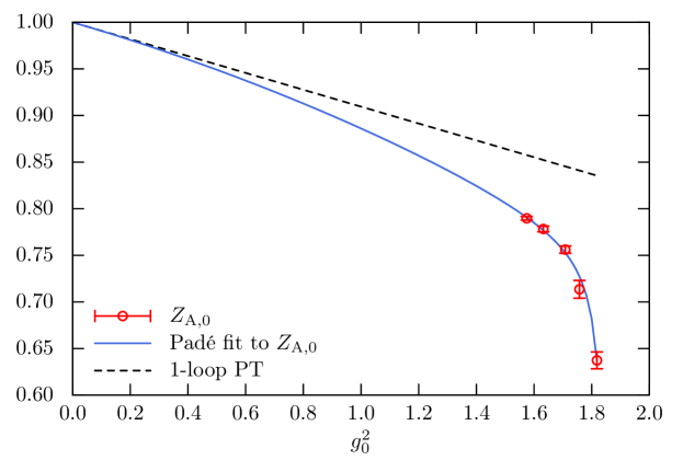
Figure 3: Final results and interpolation for $Z_{\rm A}(g_{0}^{2})=Z_{\rm A,0}(g_{0}^{2})$.

$$Z_{\rm A}(g_{0}^{2})=1-0.090488\,g_{0}^{2}\times\frac{1-0.29026\,g_{0}^{2}-0.12881\,g_{0}^{4}}{1-0.53843\,g_{0}^{2}}\;.$$ (4.12)

The associated $\chi^{2}/{\rm d.o.f.}$ is 1.71. Notice that the 1-loop perturbative formula $Z_{\rm A}(g_{0}^{2})=1-0.090488\,g_{0}^{2}$, extracted for our gauge action from the results of the calculation in [26], is imposed as asymptotic constraint. Errors at the directly simulated $\beta$-values decrease in relative size from about 1.4% at the coarsest lattice spacing (corresponding to $\beta=3.3$) to about 2.4‰ at $\beta=3.81$. It is interesting to observe that for $\beta\geq 5.5$ our interpolation formula results are consistent with those obtained in [27] for $Z_{\rm A}$ with 3 flavors of stout link non-perturbative clover fermions using a different scheme (RI’-MOM).

In our setup, an alternative definition of $Z_{\rm A}$ can be obtained by dropping the disconnected diagrams since, as discussed in Section 2, those are expected to contribute at ${\rm O}(a^{2})$ only. The results for the corresponding $Z_{\rm A}^{\rm con}$ are reproduced in Fig. 4, where they are also put in comparison to the interpolation formula in eq. (4.12) for $1.3\leq g_{0}^{2}\leq 1.9$.

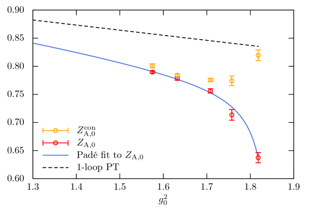
Figure 4: Comparison of $Z_{\rm A}(g_{0}^{2})$ and $Z_{\rm A}^{\rm con}(g_{0}^{2})$ for $1.3\leq g_{0}^{2}\leq 1.82$.

The difference between the two definitions amounts to a cutoff effect, and we could indeed explicitly check that it vanishes even faster than $a^{2}$. Compared to the $N_{\rm f}=2$ case in [4], we observe a much smoother, with the exceptionof the point at $a\approx 0.09\,{\rm fm}$ almost flat, dependence of $Z_{\rm A}^{\rm con}$ on $g_{0}^{2}$ at the lattice spacings considered. We ascribe that to the choice of the kinematical setup ($L\approx$ 1.2 fm) and to the approximate isolation of the ground state in the correlation functions involved, which we adopted following the suggestion put forward in [5] in order to minimize intermediate-distance cutoff effects. Indeed, as depicted in Fig. 5, we see a rather slow decay in time of the correlation function $f_{\rm P}(x_{0})$ approximately projected to the ground state, and very moderate lattice artifacts. The slope corresponds to an effective mass which is smaller than 0.3 in units of the lattice spacing, and the approximate linear behavior of the correlators in the plot implies that they are dominated by a few states (most likely one, except at very short distances), all with energies well below the cutoff scale. This is in contrast with the quite strong time-dependence observed in [28] for the correlators entering the definition of $Z_{\rm A}$. In that case, corresponding to 3 flavors of non-perturbatively improved Wilson fermions with Iwasaki gauge action, rather small volumes and wall-sources (without attempting to project on the ground state) have in fact been used.

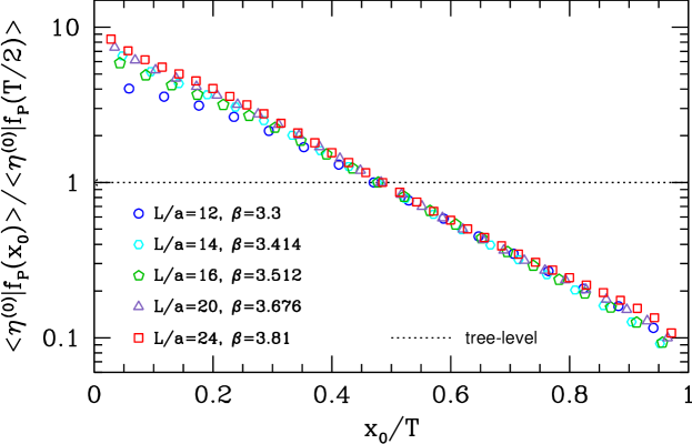
Figure 5: The correlator $f_{\rm P}(x_{0})$ projected to the approximate ground state (i.e., by taking the inner product with the associated eigenvector denoted by $\eta^{(0)}$ in [15]), for the different values of the gauge coupling along the chosen line of constant physics. Errors are of the size of the symbols and hence suppressed for better readability.

5 Conclusions

In this work we have non-perturbatively determined $Z_{\rm A}(g_{0}^{2})$, the renormalization factor of the axial vector current matrix elements, in lattice QCD with $N_{\rm f}=3$ flavors of Wilson quarks, non-perturbative $c_{\rm sw}$ [13] and the tree-level Symanzik-improved gauge action. The renormalization condition is chosen such that the Ward identities are restored up to O$(a^{2})$ at finite lattice spacing. The main result is the parameterization of $Z_{\rm A}(g_{0}^{2})$, eq. (4.12), valid for bare couplings below $g_{0}^{2}\approx 1.8$ (or, equivalently, for lattice spacings $a\lesssim 0.09\,{\rm fm}$).

As the range of lattice spacings covered in this work matches those of the large-volume $N_{\rm f}=2+1$ flavor QCD ensembles of gauge field configurations currently being generated in dynamical simulations with the same lattice action [7], the present calculation (together with the determination of the improvement coefficient $c_{\rm A}$ in [15]) is a useful ingredient in the computation of quark masses as well as of pseudoscalar meson decay constants, which can be used to convert lattice spacings to physical units and are of great phenomenological interest by their own.

Acknowledgments. We thank Rainer Sommer for helpful discussions. This work is supported by the grant HE 4517/3-1 (J. H. and C. W.) of the Deutsche Forschungsgemeinschaft. We gratefully acknowledge the computing time granted by the John von Neumann Institute for Computing (NIC) and provided on the supercomputer JUROPA at Jülich Supercomputing Centre (JSC). Computer resources were also provided by DESY, Zeuthen (PAX cluster), the CERN ‘thqcd2’ QCD HPC installation, and the ZIV of the University of Münster (PALMA HPC cluster).

References

- [1] K.G. Wilson, Confinement of quarks, Phys. Rev. D10 (1974) 2445.
- [2] M. Bochicchio, L. Maiani, G. Martinelli, G. C. Rossi and M. Testa, Chiral Symmetry on the Lattice with Wilson Fermions, Nucl. Phys. B262 (1985) 331.
- [3] M. Lüscher, S. Sint, R. Sommer and H. Wittig, Nonperturbative determination of the axial current normalization constant in improved lattice QCD, Nucl. Phys. B491 (1997) 344, hep-lat/9611015.
- [4] M. Della Morte, R. Hoffmann, F. Knechtli, R. Sommer and U. Wolff, Non-perturbative renormalization of the axial current with dynamical Wilson fermions, JHEP 0507 (2005) 007, hep-lat/0505026.
- [5] M. Della Morte, R. Sommer and S. Takeda, On cutoff effects in lattice QCD from short to long distances, Phys. Lett. B672 (2009) 407, arXiv:0807.1120.
- [6] P. Fritzsch et al., The strange quark mass and Lambda parameter of two flavor QCD, Nucl. Phys. B865 (2012) 397, arXiv:1205.5380.
- [7] M. Bruno et al., Simulation of QCD with flavors of non-perturbatively improved Wilson fermions, JHEP 1502 (2015) 043, arXiv:1411.3982.
- [8] M. Della Morte et al., Non-perturbative quark mass renormalization in two-flavor QCD, Nucl. Phys. B729 (2005) 117, hep-lat/0507035.
- [9] M. Della Morte, N. Garron, M. Papinutto and R. Sommer, Heavy quark effective theory computation of the mass of the bottom quark, JHEP 0701 (2007) 007, hep-ph/0609294.
- [10] F. Bernardoni et al., The b-quark mass from non-perturbative Heavy Quark Effective Theory at , Phys. Lett. B730 (2014) 171, arXiv:1311.5498.
- [11] M. Lüscher and P. Weisz, On-Shell Improved Lattice Gauge Theories, Commun. Math. Phys. 97 (1985) 59.
- [12] K.-I. Ishikawa et al., Mass and axial current renormalization in the Schrödinger functional scheme for the RG-improved gauge and the stout smeared -improved Wilson quark actions, PoS LATTICE2015 (2015) 271, arXiv:1511.08549.
- [13] J. Bulava and S. Schaefer, Improvement of lattice QCD with Wilson fermions and tree-level improved gauge action, Nucl. Phys. B874 (2013) 188, arXiv:1304.7093.
- [14] J. Bulava, M. Della Morte, J. Heitger and C. Wittemeier, Non-perturbative improvement and renormalization of the axial current in lattice QCD, PoS LATTICE2014 (2014) 283, arXiv:1502.07773.
- [15] J. Bulava, M. Della Morte, J. Heitger and C. Wittemeier, Non-perturbative improvement of the axial current in lattice QCD with Wilson fermions and tree-level improved gauge action, Nucl. Phys. B896 (2015) 555, arXiv:1502.04999.
- [16] M. Lüscher, S. Sint, R. Sommer and P. Weisz, Chiral symmetry and O(a) improvement in lattice QCD, Nucl. Phys. B478 (1996) 365, hep-lat/9605038.
- [17] M. Lüscher, R. Narayanan, P. Weisz and U. Wolff, The Schrödinger functional: A Renormalizable probe for non-Abelian gauge theories, Nucl. Phys. B384 (1992) 168, hep-lat/9207009.
- [18] S. Sint, On the Schrödinger functional in QCD, Nucl. Phys. B421 (1994) 135, hep-lat/9312079.
- [19] M. Dalla Brida, S. Sint and P. Vilaseca, The chirally rotated Schrödinger functional: theoretical expectations and perturbative tests, arXiv:1603.00046.
- [20] S. Sint and B. Leder, Testing universality and automatic O(a) improvement in massless lattice QCD with Wilson quarks PoS LATTICE2010 (2010) 265, arXiv:1012.2500.
- [21] M. Dalla Brida and S. Sint, A dynamical study of the chirally rotated Schrödinger functional in QCD, PoS LATTICE2014 (2014) 280, arXiv:1412.8022.
- [22] M. Lüscher and S. Schaefer, Lattice QCD with open boundary conditions and twisted-mass reweighting, Comput. Phys. Commun. 184 (2013) 519, arXiv:1206.2809.
- [23] P. Fritzsch and A. Ramos, The gradient flow coupling in the Schrödinger Functional, JHEP 1310 (2013) 008, arXiv:1301.4388.
- [24] M. Lüscher, Properties and uses of the Wilson flow in lattice QCD, JHEP 1008 (2010) 071, arXiv:1006.4518.
- [25] U. Wolff, Monte Carlo errors with less errors, Comput. Phys. Commun. 156 (2004) 143, hep-lat/0306017.
- [26] S. Aoki, K. I. Nagai, Y. Taniguchi and A. Ukawa, Perturbative renormalization factors of bilinear quark operators for improved gluon and quark actions in lattice QCD, Phys. Rev. D 58 (1998) 074505, hep-lat/9802034.
- [27] M. Constantinou, R. Horsley, H. Panagopoulos, H. Perlt, P. E. L. Rakow, G. Schierholz, A. Schiller and J. M. Zanotti, Renormalization of local quark-bilinear operators for flavors of stout link nonperturbative clover fermions, Phys. Rev. D 91 (2015) no.1, 014502, arXiv:1408.6047.
- [28] S. Aoki et al. [PACS-CS Collaboration], Non-perturbative renormalization of quark mass in QCD with the Schroedinger functional scheme, JHEP 1008 (2010) 101, arXiv:1006.1164.