A copula-based model for multivariate ordinal panel data:
application to well-being composition
Abstract
A novel copula-based multivariate panel ordinal model is developed to estimate structural relations among components of well-being. Each ordinal time-series is modelled using a copula-based Markov model to relate the marginal distributions of the response at each time of observation and then, at each observation time, the conditional distributions of each ordinal time-series are joined using a multivariate t copula. Maximum simulated likelihood based on evaluating the multidimensional integrals of the likelihood with randomized quasi Monte Carlo methods is used for the estimation. Asymptotic calculations show that our method is nearly as efficient as maximum likelihood for fully specified multivariate copula models. Our findings highlight the importance of one’s relative position in evaluating their well-being with no direct effects of socio-economic characteristics on well-being but strong indirect effects through their impact on components of well-being. Temporal resilience, habit formation and behavioural traits can explain the dependence in the joint tails over time and across well-being components.
JEL classification: C33; C51; C61
Keywords: Panel ordinal data; Simulated likelihood; Markov models; Joint tail probabilities; Well-being composition
1 Introduction
Subjective well-being and life satisfaction have received a significant amount of attention in the economics (Blanchflower and Oswald,, 2004; Ferrer-i Carbonell and Frijters,, 2004) and psychology (Diener et al.,, 1999; Argyle,, 1999) literature over the past decades. While cardinality properties are conceptually rejected, the ordinal nature of the information conveyed in such indicators has gradually entered public policy circles. Stiglitz et al., (2009) argued that meaningful and reliable data on well-being can be collected and should be included in surveys and official statistics with further reports advocating its role in policy making in informing policy designs, monitoring progress and evaluating implementation of public interventions (Dolan and Metcalfe,, 2012).
However, despite suggestions by various authors (Cummins et al.,, 2003; Kahneman and Krueger,, 2006; Krueger and Schkade,, 2008; Veenhoven,, 2013), there is little consensus in how exactly such concepts are defined and what precisely they capture. For the past few years the Office for National Statistics in the UK monitors year-on-year improvements in reported well-being through questions on life satisfaction, feelings of self-worth, happiness and anxiety, which however provides little theoretical basis or conceptual background for such choices (ONS,, 2014). While it is clear that well-being is less of an answer to a single question and more of a composite multidimensional concept, limited empirical work has pursued such considerations. The vast majority of empirical work (for reviews see Kahneman and Krueger, (2006); Dolan et al., (2008)) focuses on univariate models that would not allow taking into account dependence between constituent components and their link with overall happiness, while also being unable to correctly identify direct effects of independent determinants/variables on domain and generic happiness in the presence of such outcomes’ dependence. In our context, generic well-being or happiness pertains to one’s satisfaction with their life overall, while domain well-being/satisfaction pertains to satisfaction individual constituent components of life, e.g. income, health, social life, family life, etc.
Conceptual work suggests bottom-up theories (Diener,, 1984) for life-satisfaction where judgements are based on assessments of satisfaction with a number of defined life domains with ensuing causal pathways running from the domains upwards (Schimmack,, 2008). Complementary positions view overall life satisfaction as the net outcome of reported satisfaction with life domains with the domains themselves seen as functions of objective outcomes/situations/covariates (Michalos,, 1991; Easterlin and Sawangfa,, 2008). Looking at the structure of composite well-being, Salvatore and Sastre, (2001) conclude it is more easily interpreted in terms of generic dimensions of life (e.g. family life, social life, love life, occupational life and leisure) than attributed to the fulfilment of personal values (self-acceptance, autonomy, environmental mastery, purpose in life, and personal growth). Brief et al., (1993) argued for a mixture of processes where individual characteristics and traits are driving domain satisfaction (i.e. top-down), which in turn drives life satisfaction (i.e. bottom-up). In other words, high individual income leads to increased life satisfaction because financial satisfaction is an important component of satisfaction with life as a whole.
Looking at the economics of well-being literature, univariate models again dominate, while at the same time very few studies have focused on its composite structure. van Praag et al., (2003) formulate a model very close to the initial bottom-up theories, which however is estimable only under strong assumptions of no direct association between individual covariates and generic life satisfaction. However, problems of omitted variables and lack of sufficient exclusion restrictions suggest caution in drawing conclusions. Similar problems are also faced in Easterlin and Sawangfa, (2008), where again strong assumptions (both conceptual and econometric) are required in the model and raise concerns about the robustness of findings.
However, most theories developed within the well-being composition literature offer limited empirical evidence for the underlying connections posited and fail to explicitly incorporate them into their setting. In this paper we propose a multivariate framework and estimate a comprehensive relationships pattern between generic and domain satisfactions with dependence explicitly modelled through copulas. We develop a novel joint copula-based Markov model, where a set of bivariate copulas and a multivariate t (MVT) copula jointly model multivariate ordinal time-series responses with covariates. Each ordinal time-series is considered a copula-based Markov model, where a parametric bivariate copula family is used for the joint distribution of subsequent observations and which is then related to these ordinal time-series responses using an MVT to join their conditional (on the past) distributions at each time point. Note in passing that other continuous-variable models using copulas in several Markov chains exist in the literature (Lambert and Vandenhende,, 2002; Patton,, 2012; Rémillard et al.,, 2012; Beare and Seo,, 2015), but in our knowledge we are the first constructing such copula-based models for ordinal time-series with covariates. The theoretical and estimation concepts in the discrete case are quite different.
Simple parametric families of copulas in more than two dimensions typically provide limited dependence (Nikoloulopoulos, 2013a, ) and for discrete data it is generally hard to provide a better fit than the multivariate normal (MVN) copula, which inherits the useful properties of the MVN distribution. However, the MVN copula is inadequate to model multivariate data with more probability in one or both joint tails. In recent years, a popular and useful approach is the vine pair-copula construction (Kurowicka and Joe,, 2011; Nikoloulopoulos et al.,, 2012) which is based on bivariate copulas, of which some are used to summarize conditional dependence. Vine copula constructions are suitable for modelling this kind of data by using appropriate bivariate copulas. Panagiotelis et al., (2012) and Nikoloulopoulos and Joe, (2015) recently extended the idea of vine copulas to discrete data. The approach in Nikoloulopoulos and Joe, (2015) involves both observed and latent variables, while the approach of Panagiotelis et al., (2012) is suitable when there are no latent variables to explain the dependence in the observed variables. In this paper to form the bivariate part of the model, a D-vine truncated at the 1-st level (Brechmann et al.,, 2012) has been exploited.
To develop the joint copula-based Markov model we propose the MVT copulas. MVT copulas nest MVN copulas and share with them the ability to accommodate any feasible pattern of association in a set of random variables. However, the MVT copulas offer greater flexibility than MVN copulas, as they can also capture dependence in both joint tails (Nikoloulopoulos et al.,, 2009), which is the case in ‘mixtures’ of population (e.g., different locations or genders). The MVT copula-based approach of this article avoids having to specify parametrically the distribution of latent heterogeneity in a non-linear setting. The MVT copulas as scale mixtures of MVN can be used to explore unobserved population heterogeneity.
Implementation of the MVT copula for discrete data is feasible, but not easy, because the MVT distribution, as a latent model for discrete response, requires rectangle probabilities based on high-dimensional integrations (Genest et al.,, 2013). The probability mass function (pmf) can be obtained by computing an MVT rectangle probability and the randomized quasi Monte Carlo methods proposed by Genz and Bretz, (2002) can be used for that purpose. Computing the rectangle MVT probabilities via simulation based on the methods in Genz and Bretz, (2002) is akin to using a simulated likelihood method, whose asymptotic efficiency, for the special case of MVN copula, has been studied by Nikoloulopoulos, 2013b ; Nikoloulopoulos, 2016b and was shown to be as good as maximum likelihood for dimension 10 or lower.
Modelling of dependence further allows revisiting a number of established relationships in the literature between covariates and well-being and examining their association in a multivariate setting (e.g. does the importance of income on generic well-being remain when considered along income satisfaction?). In short, we establish exogenous determinants for both generic and domain satisfaction equations and separately identify structural relations among components of well-being and shed light not only into their links with generic well-being but also among themselves. This allows separate identification of the direct effect of domain characteristics and of composite domains on generic satisfaction, as well as estimation of the dependence between and among generic and domain satisfaction.
Prokhorov and Schmidt, (2009) showed that robust estimation can be achieved in the class of radially or reflection symmetric copulas such as the normal or t copula. Nikoloulopoulos et al., (2011), Masarotto and Varin, (2012), Nikoloulopoulos, 2016a and Nikoloulopoulos, 2016c (in particular for ordinal time-series) showed robustness of the normal copula to dependence if the main interest is the univariate parameters (regression and nonregression parameters). This type of research focussed on marginal models and on estimation of coefficients for regression models with time-series data, that are robust to the dependence structure. Nevertheless, our manuscript is not entirely in the area of “marginal models” (meaning specification of univariate time-series only), but also avails copula-based models for both univariate and multivariate time-series. One of the goals of our paper is to compare dependence models in inferences involving joint probabilities.
The remainder of the paper proceeds as follows. Section 2 introduces the joint copula-based Markov model for discrete ordinal responses with covariates and presents the conceptual framework upon which this econometric model is built. Estimation techniques and computational details are provided in Section 3. Section 4 discusses the Vuong’s (1989) test to assess the fit of the proposed model in terms of prediction of joint probabilities. Section 5 presents the application of our methodology to the British Household Panel and Section 6 concludes, followed by a technical Appendix.
2 A joint copula-based Markov model
In this section, we construct the joint copula-based Markov model for ordinal time-series with covariates. Before that, the first subsection has some background on copula models.
2.1 Overview and relevant background for copulas
A copula is a multivariate cdf with uniform margins (Joe,, 1997, 2014; Nelsen,, 2006). If is a -variate cdf with univariate margins , then Sklar’s (1959) theorem implies that there is a copula such that
The copula is unique if are continuous, but not if some of the have discrete components. If is continuous and , then the unique copula is the distribution of leading to
where are inverse cdfs. In particular, if is the MVT cdf with correlation matrix and degrees of freedom, and is the univariate Student t cdf with degrees of freedom, then the MVT copula is
| (1) |
2.2 Copula-based Markov models for ordinal time-series
For a latent variable such that if with being the number of categories of , the -dimensional regression vector, the “panel” dimension, the number of clusters (note that varying cluster sizes can be accommodated by the theory) and the number of covariates (i.e. the dimension of a covariate vector ), the response is assumed to have density
where is a function of , is a -dimensional regression vector and is the -dimensional vector of the univariate cutpoints () with and . Choosing normal or logistic for leads to the ordered probit and cumulative logit models, respectively.
For data , where is an index for the ordinal responses, the univariate marginal model for is where and of dimension . If for each , are independent, then the log-likelihood for each univariate ordinal response is
| (2) |
If the ordinal data are observed in a time-series sequence, then the ordinal regression model can be adapted in two ways:
-
1.
add previous observations as covariates;
-
2.
make use of some models for stationary ordinal time-series.
Here we adapt the methodology for case 2. For dependent , estimation of and involves copula-based Markov models (Joe,, 1997, page 244) for ordinal time-series with covariates. The joint distribution of subsequent observations is modelled through a parametric copula family with the corresponding transition probabilities subsequently elicited. The advantages of a time-series regression model are explicitly mentioned in Joe, (2015) and also reproduced below:
-
•
The class of autocorrelation functions is much wider than those based on an ordered probit with lagged dependent variables appearing as explanatory variables.
-
•
Prediction in regressions with time dependent observations is simpler as they can be formulated with or without the preceding observations.
-
•
Serial dependence (positive or negative) can be modelled through suitable copula families.
-
•
The non-linearity of the conditional expectations allows for various patterns to be replicated, while the conditional expectation and variance for large values is determined by the choice of copula family and corresponding tail behaviour.
-
•
Incorporating covariates in time-series models is more straightforward in univariate regression models.
-
•
Extending the framework to Markov orders higher than one is straightforward.
-
•
Copula families with an easy (e.g. closed) form allow for easier likelihood inference.
Note in passing that copula-based Markov models for continuous response data have been studied before in Chen and Fan, (2006).
Assuming a copula based Markov model, the transition cdf of given is
and the transition pmf is
where . Then the log-likelihood for each ordinal time-series is
| (4) |
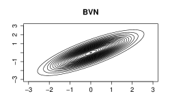
Such framework incorporates the BVN copula as a special case, i.e. “autoregressive-to-anything” in Biller and Nelson, (2005) as also acknowledged by Joe, (2014). Stronger clustering of consecutive large/small values than expected in the BVN would require alternative copulas to obtain more appropriate transition probabilities.
2.2.1 Choices of parametric families of copulas
In our candidate set, families that are in line with the conditions under which a copula function generates a stationary Markov chain that satisfies mixing conditions at a geometric rate (Chen et al.,, 2009; Beare,, 2010) are used. These families have different strengths of tail behaviour (see e.g., Nikoloulopoulos et al., (2012); Nikoloulopoulos and Joe, (2015)): 333A bivariate copula is reflection symmetric if its density satisfies for all and reflection asymmetric otherwise often with more probability in the joint upper tail or joint lower tail. Upper tail dependence implies as and lower tail dependence that as . If for a bivariate copula , then , with being the survival (or rotated by 180 degrees) copula of . The “reflection” of each uniform random variable by about changes the direction of tail asymmetry.
-
•
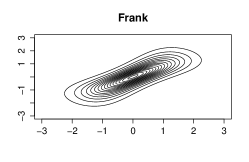
Frank copula is reflection symmetric satisfying tail independence and as , with cdf
-
•
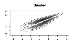
Gumbel extreme value copula is reflection asymmetric with upper tail dependence and cdf
Compared to the BVN copula, the resulting model has more probability in the joint upper tail accommodating more dependence of large ordinal values than expected in the BVN.
-
•
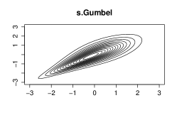
Survival Gumbel (s.Gumbel) copula is reflection asymmetric with lower tail dependence and cdf
Compared to the BVN copula, this resulting model has more probability in the joint lower tail accommodating more dependence of small ordinal values than expected in the BVN.
-
•
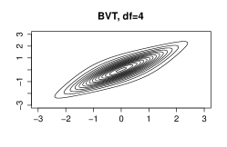
Bivariate Student t (BVT) copula with reflection symmetric upper and lower tail dependence and cdf
where is the univariate Student t cdf with (non-integer) degrees of freedom, and is the cdf of a bivariate Student t distribution with degrees of freedom and correlation parameter . Small values of (i.e. ) lead to models with more probabilities in the joint upper and joint lower tails accommodating more dependence of large and small ordinal values that would be expected with BVN.
Nikoloulopoulos and Karlis, (2008) have shown that, when using real data, copulas with similar (tail) dependence properties provide similar fit making selection among them cumbersome. With tail dependence properties being copula family specific, upper/lower tail dependence becomes one way to differentiate among families. Contour plots of copula densities with standard normal margins and dependence parameters corresponding to Kendall’s are given in Figure 1 to depict concepts of reflection (a)symmetric tail (in)dependence.
 |
 |
 |
|
 |
 |
2.3 Joint copula-based Markov models for ordinal time-series
So far we treat the ordinal time-series responses separately as if they were independent. In this Section, we propose relating these responses using an MVT copula to join their conditional (on the past) distributions at each time point.
Consider a multivariate discrete regression setup in which the dependent ordinal time-series are observed together with a vector of explanatory variables. If is the MVT copula (or any other parametric family of copulas) and , as defined in (2.2), is the parametric model for the th univariate ordinal time-series then
is a multivariate parametric model with univariate margins . For copula models, the response vector can be discrete (Nikoloulopoulos, 2013a, ; Nikoloulopoulos and Joe,, 2015).
Then it follows that the joint pmf is
where , and denotes the MVT density with latent correlation matrix and degrees of freedom. The MVN case can be treated as a special case of the MVT with a large value of .
For the joint copula-based Markov model, we let and be parametric bivariate copulas, say with parameters and be an MVT copula. For the set of all parameters, let . We model the joint distribution in terms of bivariate copulas and an MVT copula. Note that the copula models the time-series for the th response and the copula links that ordinal time-series responses. Our general statistical model allows for selection of independently among a variety of parametric copula families, i.e., there are no constraints in the choices of parametric copulas .
2.4 Conceptual framework
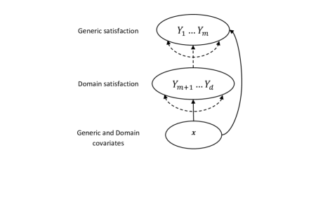
Let and denote the generic and domain satisfactions, respectively. We propose an expansive set of relationships: objective individual characteristics and covariates directly relate to both generic and domain satisfactions, with further influencing , while inter-dependencies among them are also allowed. Such latent correlations capture the residual dependence (i.e. over and above the effect of covariates) among equations/outcomes. Figure 2 gives a schematic of our structural model. Such specification allows for direct, indirect and ripple (spill-over) effects on well-being, e.g. capturing at least three possible ways high individual income could affect generic satisfaction: a) a direct effect of income, b) an indirect effect through income satisfaction and c) an indirect effect through increased income satisfaction that itself is the result of an improved, for example, leisure satisfaction that was caused by the initial increase in income.
 |
3 Estimation techniques and computational details
For estimation purposes we propose a maximum simulated likelihood method, which is based on evaluating the multidimensional integrals of the likelihood with randomized quasi Monte Carlo methods; an analysis of asymptotic properties of the estimators is shown in the Appendix.
3.1 Simulated likelihood
We develop and implement a maximum simulated likelihood estimator (MSLE). There exist general results on asymptotics of simulated likelihood based estimators (see, e.g., Gouriéroux and Monfort,, 1991). They usually involve a rate assumption on the number of simulations versus the sample size. Nevertheless, we propose a simulated likelihood method, where the rectangle MVT probabilities in (2.3) and (6) are computed using a quasi Monte Carlo method proposed by Genz and Bretz, (2002). Genz and Bretz, (2002) achieve error reduction of Monte Carlo methods through variance reduction techniques such as (a) transforming to a bounded integrand, (b) using antithetic variates, and (c) using a randomized quasi Monte Carlo method. The test results in Genz and Bretz, (2002, 2009) show that their method is very efficient, compared to other methods in the literature. The method in Genz and Bretz, (2002) is “optimized” in the mtvnorm R package (Genz et al.,, 2012). Hence, on the calculation of the MSLE, one doesn’t need to worry about the selection, for example, of the number of simulated quasi points.
The estimated parameters can be obtained by maximizing the simulated log-likelihood in (5) over the model parameters . The method was initially proposed for the analysis of discrete (binary and count) longitudinal data by Nikoloulopoulos, 2013b and extended to a high-dimensional context in Nikoloulopoulos, 2016b . We refer the interested reader to these papers for more details including studies of small-sample and asymptotic efficiency for Bernoulli, Poisson, and negative binomial regression models. In addition to that we study here the asymptotic properties of the maximum simulated likelihood estimators for ordinal regression models in an Appendix.
3.2 Computational details
The MSLEs can be derived using a three-step procedure:
-
1.
For each :
-
(a)
Assuming time independence, in (2) is maximized over the univariate marginal parameters .
-
(b)
Keeping the univariate parameters fixed at the values estimated in (a), the in (4) is maximized over the copula parameter .
-
(c)
Finally, using starting values from the estimates above the in (4) is maximized over both the univariate and copula parameters.
-
(a)
-
2.
Setting all parameters to their estimated values from the first step, the in (5) is maximized over .
-
3.
At the third and final step the in (5) is maximized over with initial parameters the estimates for the preceding steps.
Given the typical large number of estimable (univariate and copula) parameters in multivariate models one can restrict themselves to only the first two steps of the method to make inference computationally feasible. This two-step approach is known in the copula literature as the Inference Function of Margins (IFM) method (Joe and Xu,, 1996; Joe,, 1997) and its asymptotic efficiency has been established (Joe,, 2005). Hence using only the two first steps,
-
•
the model parameters can be efficiently (in the sense of computing time and asymptotic variance) estimated;
-
•
cross-model comparisons with respect to dependence structure and subsequently predictions and inferences can be performed.
Note also in passing that compared to the (simulated) maximum likelihood, the IFM method is not as punishing for misspecification of the dependence structure (Joe and Xu,, 1996; Xu,, 1996).
Each of the estimated parameters can be obtained by using a quasi-Newton (Nash,, 1990) method applied to the log-likelihood. This numerical method requires only the objective function, i.e., the joint log-likelihood, while the gradients are computed numerically and the Hessian matrix of the second order derivatives is updated in each iteration. Since the estimation of parameters in MVT copula-based models is obtained using a quasi-Newton routine (Nash,, 1990) applied to the log-likelihood in (5), the use of randomized quasi Monte Carlo simulation to four decimal place accuracy for evaluations of integrals works poorly, because numerical derivatives of the log-likelihood with respect to the parameters are not smooth. In order to achieve smoothness, the same set of uniform random variables should be used for every rectangle probability that comes up in the optimization of the simulated likelihood (Nikoloulopoulos, 2013b, ; Nikoloulopoulos, 2016b, ).
4 Vuong’s test for model comparison
A methodology for the comparison of non-nested models using the Vuong’s test (Vuong,, 1989) is formulated below to test if:
-
1.
the copula-based Markov models with different choices of bivariate copulas outperform the copula-based Markov model with BVN (i.e. “autoregressive-to-anything” model);
-
2.
the joint copula-based Markov models with MVT copulas provide better fit than their special case, namely the MVN copula.
The Vuong’s test is appropriate for parametric non-nested models comparisons and has often been used in the copula literature (e.g., Belgorodski,, 2010; Brechmann et al.,, 2012; Joe,, 2014; Nikoloulopoulos,, 2015).
Assume models 1 and 2 with parametric densities and , respectively. Comparison of
and
where are the parameters in models 1 and 2 respectively that lead to the closest Kullback-Leibler divergence to the true . Model 1 is closer to the true , i.e., fits better if , while model 2 fits better if . The sample version of with estimates is
where .
Vuong, (1989) has shown that asymptotically under the null hypothesis , i.e., models 1 and 2 have the same parametric densities and ,
where . Rejection on the null hypothesis follows if is greater than the critical value from the standard normal distribution, denoted .
5 British Household Panel Survey
For the estimation of the model in Figure 2 we use data from the British Household Panel Survey (BHPS). The BHPS was an annual longitudinal survey (now superseded by Understanding Society) carried out by the Institute for Social and Economic Research sampling about 10,000 individuals aged 16 years or over from 1991 to 2008. However, the survey modules required for our model are collected on a bi-annual basis starting in wave 6 (i.e. 1996) and finishing in wave 18 (i.e. 2008), resulting in a maximum of 7 measurements per individual. To ease coding, we use individuals observed at all seven time points resulting in a sample size of 4186 individuals, though our methodology does not depend on a constant “cluster” size .
5.1 Equations and covariates
The actual model estimated is based on one generic and six domain satisfaction questions each answered on a 1 (not satisfied at all) to 6 (completely satisfied) likert scale. The seven equations (outcomes) are:
- :
-
Satisfaction with Life overall
- :
-
Satisfaction with Health
- :
-
Satisfaction with Income
- :
-
Satisfaction with House/flat
- :
-
Satisfaction with Spouse/partner
- :
-
Satisfaction with Job
- :
-
Satisfaction with Leisure
Each of is conditioned upon individual characteristics (i.e. age, age square, gender, household size, number of kids, education and geographical region within the UK) that are common controls in the well-being literature and domain specific factors that appear only on the respective domain equation and would enhance the ability to capture domain specific variation. For example, number of health problems are used for the satisfaction with health equation, disaggregated sources of income in the satisfaction with income equation and so on for the rest of the equations. Table 1 offers definitions and breakdowns for domain specific variables, as well as the reference levels for all categorical variables. Note that the original region variable is a geographical identifier that splits UK into 19 areas and which is aggregated into 5 “super”-regions for the regressions. Further, income rank captures relative income and is determined by the rank of the individual in their original region (i.e. one of 19 areas) according to their total annual income.
For equation we use as covariates all common and domain specific variables capturing the direct effects that each characteristic has on overall life satisfaction. This formulation allows the separate identification of the direct effect of domain characteristics and the effect of composite domains on generic satisfaction, while, as the econometric model poses, residual dependence between and among and is captured by estimable latent correlation parameters.
Given the multivariate nature of our model we restrict the estimation sample to those for whom information on each equation is available, i.e. married, employed individuals (up to 70 years old) who indicate to have a partner. Further, as discussed earlier, albeit not a requirement of the model, we only keep those individuals that appear in all seven waves of the data. Descriptive statistics for all equation outcomes, and covariates are available in Table 1 where informal sample selection comparisons can also be drawn between the estimation and full sample. Respondents tend to be most satisfied with their partners, followed by satisfaction with their houses and then with life overall. Income and leisure are the least satisfactory dimensions. Overall, our sample is 46% males and on average 45 years old, with 12% having a higher degree and 7% residing in London, 20% in South England, 16% in the Midlands and 19% in North England. Comparing restricted and full samples the former is slightly less educated and with a different income sources structure but on average individual characteristics and domain covariates are largely comparable across the two samples.
| Estimation sample | Full sample | ||
| Equations | |||
| : Satisfaction with Life overall | 4.25 | 4.29 | |
| : Satisfaction with Health | 4.00 | 4.23 | |
| : Satisfaction with Income | 3.64 | 3.78 | |
| : Satisfaction with House/flat | 4.45 | 4.44 | |
| : Satisfaction with Spouse/partner | 5.24 | 5.27 | |
| : Satisfaction with Job | 4.05 | 4.01 | |
| : Satisfaction with Leisure | 3.93 | 3.77 | |
| Covariates | |||
| Age | 4.53 | 4.36 | |
| Age2 | 23.98 | 19.72 | |
| Sex (1 if male) | 0.46 | 0.55 | |
| Household size | 0.29 | 0.33 | |
| # of kids | 0.06 | 0.09 | |
| Education (ref category: Uni degree) | |||
| hnd,hnc, a/o levels, cse | 0.55 | 0.69 | |
| No education | 0.33 | 0.11 | |
| Region (ref category: London) | |||
| South | 0.20 | 0.30 | |
| Midlands | 0.16 | 0.22 | |
| North | 0.19 | 0.32 | |
| RUK | 0.38 | 0.10 | |
| Health | |||
| # Health problems | 0.12 | 0.08 | |
| Income | |||
| ln(Labour Income) | 7.53 | 10.47 | |
| ln(Pension Income) | 1.98 | 0.68 | |
| ln(Benefit Income) | 5.89 | 4.80 | |
| ln(Transfer Income) | 0.70 | 0.41 | |
| ln(Investment Income) | 3.46 | 4.19 | |
| Regional incomne rank (stadardized) | 0.00 | -0.07 | |
| House type (ref category: Detached) | |||
| Semi-detached | 0.32 | 0.43 | |
| Terraced | 0.27 | 0.21 | |
| Other | 0.15 | 0.02 | |
| House value (ref category: 0-50K) | |||
| 50K-100K | 0.35 | 0.28 | |
| 100K-175K | 0.23 | 0.25 | |
| 175K-250K | 0.14 | 0.19 | |
| 250K | 0.11 | 0.15 | |
| Continued on next page | |||
| Estimation sample | Full sample | ||
|---|---|---|---|
| Spouse Charateristics | |||
| Age of spouse | 4.70 | 4.37 | |
| Age2 of spouse | 24.46 | 19.92 | |
| Sex of spouse | 0.50 | 0.45 | |
| Education (ref category: Uni degree) | |||
| hnd,hnc, a/o levels, cse | 0.55 | 0.67 | |
| No education | 0.32 | 0.16 | |
| ln(Labour Income) | 6.35 | 8.46 | |
| # Health problems | 0.11 | 0.09 | |
| Hours of wk housework | 1.19 | 1.18 | |
| Satisfaction with job pay (ref category: Low) | |||
| Medium | 0.33 | 0.33 | |
| Very | 0.45 | 0.49 | |
| Satisfaction with job security (ref category: Low) | |||
| Medium | 0.26 | 0.31 | |
| Very | 0.61 | 0.57 | |
| Satisfaction with work itself (ref category: Low) | |||
| Medium | 0.28 | 0.30 | |
| Very | 0.62 | 0.61 | |
| Satisfaction with hours worked (ref category: Low) | |||
| Medium | 0.31 | 0.33 | |
| Very | 0.54 | 0.51 | |
| Leisure activities (1 if several times a year) | |||
| walk/swim/play sport | 0.67 | 0.75 | |
| watch live sport | 0.25 | 0.33 | |
| cinema | 0.47 | 0.53 | |
| theatre/concert | 0.36 | 0.37 | |
| out for a drink | 0.69 | 0.84 | |
| work in garden | 0.64 | 0.86 | |
| diy, car maintenance | 0.53 | 0.72 | |
| attend evening classes | 0.27 | 0.30 | |
| attend local groups | 0.20 | 0.21 |
5.2 Fitted copula-based Markov models for each ordinal time-series
We fit the copula-based Markov model with BVN, Gumbel, s.Gumbel, and BVT bivariate linking copulas. For BVT, choices of were . To make it easier to compare the dependence parameters, we convert the estimated parameters to Kendall’s ’s in via the relations , and for elliptical, Frank and Gumbel copulas in Hult and Lindskog, (2002), Genest, (1987), and Genest and MacKay, (1986), respectively. Note that Kendall’s tau only accounts for the dependence dominated by the middle of the data, and it is expected to be similar amongst different families of copulas. However, the tail dependence varies, as explained in Section 2.2.1, and is a property to consider when choosing amongst different families of copulas. For the model with BVT we summarize the choice of integer with the largest log-likelihood.
Given the equality in number of parameters between models, the log-likelihood at estimates can be used as a measure for goodness of fit across all models. We further compute the Vuong’s (1989) test to formally assess if more probability is accumulated in the joint tails than one would expect via a BVN copula.
For these data, if a respondent thinks about the maximum or minimum satisfaction at year it seems natural to think about the maximum or minimum satisfaction at year and year . That is, based on data descriptions, we could expect a priori that a model with being the BVT copulas might be plausible, as data have more probability in the joint tails.
| BVN | Frank | Gumbel | s.Gumbel | BVT, | ||||
| Est. | Est. | Est. | Est. | Est. | SE | -value | ||
| -2.93 | -3.24 | -2.88 | -2.63 | -2.63 | 0.83 | -3.18 | 0.01 | |
| -2.07 | -2.38 | -1.98 | -1.90 | -1.81 | 0.82 | -2.20 | 0.03 | |
| -1.33 | -1.64 | -1.22 | -1.23 | -1.09 | 0.82 | -1.32 | 0.19 | |
| -0.14 | -0.47 | -0.03 | -0.09 | 0.09 | 0.83 | 0.11 | 0.92 | |
| 1.44 | 1.10 | 1.48 | 1.50 | 1.66 | 0.83 | 2.01 | 0.04 | |
| Age | -0.74 | -0.84 | -0.58 | -0.70 | -0.55 | 0.31 | -1.79 | 0.07 |
| Age2 | 0.10 | 0.11 | 0.08 | 0.10 | 0.08 | 0.03 | 2.23 | 0.03 |
| Sex | 0.13 | 0.45 | 0.32 | -0.09 | 0.08 | 0.37 | 0.20 | 0.84 |
| Household size | -0.72 | -0.70 | -0.78 | -0.64 | -0.70 | 0.32 | -2.16 | 0.03 |
| # of kids | 0.10 | 0.01 | -0.03 | 0.08 | -0.03 | 0.34 | -0.10 | 0.93 |
| Education | ||||||||
| No education | 0.08 | 0.09 | 0.09 | 0.11 | 0.11 | 0.11 | 1.06 | 0.29 |
| hnd,hnc, a/o levels, cse | 0.03 | 0.03 | 0.05 | 0.03 | 0.05 | 0.07 | 0.73 | 0.46 |
| Region | ||||||||
| South | 0.22 | 0.25 | 0.28 | 0.18 | 0.24 | 0.11 | 2.08 | 0.04 |
| Midlands | 0.12 | 0.18 | 0.17 | 0.09 | 0.12 | 0.12 | 1.03 | 0.30 |
| North | 0.16 | 0.15 | 0.22 | 0.16 | 0.21 | 0.12 | 1.82 | 0.07 |
| RUK | 0.30 | 0.32 | 0.29 | 0.31 | 0.29 | 0.16 | 1.85 | 0.07 |
| Health | ||||||||
| # Health problems | -1.43 | -1.53 | -1.46 | -1.24 | -1.34 | 0.19 | -7.05 | 0.00 |
| Income | ||||||||
| ln(Labour Income) | 0.05 | 0.01 | 0.03 | 0.07 | 0.05 | 0.06 | 0.95 | 0.34 |
| ln(Pension Income) | 0.01 | 0.00 | 0.00 | 0.00 | 0.00 | 0.01 | 0.20 | 0.84 |
| ln(Benefit Income) | -0.01 | -0.00 | -0.01 | -0.01 | -0.01 | 0.01 | -1.01 | 0.31 |
| ln(Transfer Income) | -0.01 | -0.01 | -0.01 | -0.00 | -0.00 | 0.01 | -0.29 | 0.77 |
| ln(Investment Income) | 0.01 | 0.01 | 0.01 | 0.01 | 0.01 | 0.01 | 1.29 | 0.20 |
| Regional income rank (standardized) | -0.01 | 0.02 | 0.01 | -0.03 | -0.02 | 0.05 | -0.33 | 0.74 |
| House type | ||||||||
| Semi-detached | -0.03 | -0.049 | -0.04 | -0.04 | -0.04 | 0.05 | -0.80 | 0.42 |
| Terraced | -0.09 | -0.12 | -0.09 | -0.11 | -0.10 | 0.07 | -1.56 | 0.12 |
| Other | -0.45 | -0.44 | -0.41 | -0.44 | -0.43 | 0.15 | -2.80 | 0.01 |
| House value | ||||||||
| 50K-100K | -0.06 | -0.03 | -0.06 | -0.07 | -0.07 | 0.06 | -1.21 | 0.23 |
| 100K-175K | -0.12 | -0.07 | -0.10 | -0.15 | -0.13 | 0.07 | -1.79 | 0.07 |
| 175K-250K | -0.15 | -0.12 | -0.12 | -0.17 | -0.15 | 0.08 | -1.82 | 0.07 |
| 250K | -0.12 | -0.09 | -0.09 | -0.14 | -0.12 | 0.10 | -1.20 | 0.23 |
| Spouse Charateristics | ||||||||
| Age | 0.07 | -0.03 | 0.03 | 0.07 | 0.04 | 0.28 | 0.13 | 0.90 |
| Age2 | -0.03 | -0.01 | -0.02 | -0.03 | -0.03 | 0.03 | -0.81 | 0.42 |
| Sex | 0.13 | 0.46 | 0.31 | -0.07 | 0.08 | 0.37 | 0.22 | 0.83 |
| Education | ||||||||
| No education | 0.10 | 0.06 | 0.10 | 0.12 | 0.12 | 0.10 | 1.16 | 0.25 |
| hnd,hnc, a/o levels, cse | -0.05 | -0.03 | -0.09 | -0.04 | -0.09 | 0.07 | -1.15 | 0.25 |
| ln(Labour Income) of spouse | 0.01 | 0.01 | 0.01 | 0.01 | 0.01 | 0.01 | 1.17 | 0.24 |
| # Health problems of spouse | -0.27 | -0.25 | -0.19 | -0.26 | -0.19 | 0.17 | -1.11 | 0.27 |
| Hours of wk housework | -0.02 | -0.02 | -0.02 | -0.01 | -0.01 | 0.02 | -0.54 | 0.59 |
| Satisfaction with job pay | ||||||||
| Medium | 0.14 | 0.18 | 0.15 | 0.13 | 0.14 | 0.04 | 3.15 | 0.00 |
| Very | 0.23 | 0.28 | 0.22 | 0.20 | 0.20 | 0.05 | 4.44 | 0.00 |
| Satisfaction with job security | ||||||||
| Medium | 0.10 | 0.10 | 0.09 | 0.11 | 0.10 | 0.05 | 2.14 | 0.03 |
| Very | 0.18 | 0.18 | 0.16 | 0.17 | 0.16 | 0.05 | 3.42 | 0.00 |
| Satisfaction with work itself | ||||||||
| Medium | 0.14 | 0.16 | 0.12 | 0.14 | 0.14 | 0.05 | 2.62 | 0.01 |
| Very | 0.41 | 0.41 | 0.37 | 0.39 | 0.38 | 0.05 | 7.03 | 0.00 |
| Continued on next page | ||||||||
| BVN | Frank | Gumbel | s.Gumbel | BVT, | ||||
| Est. | Est. | Est. | Est. | Est. | SE | -value | ||
| Satisfaction with hours worked | ||||||||
| Medium | 0.21 | 0.19 | 0.19 | 0.20 | 0.19 | 0.04 | 4.32 | 0.00 |
| Very | 0.32 | 0.29 | 0.30 | 0.29 | 0.30 | 0.05 | 6.21 | 0.00 |
| Frequency of leisure activities | ||||||||
| walk/swim/play sport | -0.02 | 0.00 | -0.02 | -0.03 | -0.04 | 0.04 | -1.07 | 0.29 |
| watch live sport | 0.06 | 0.06 | 0.05 | 0.06 | 0.05 | 0.04 | 1.18 | 0.24 |
| cinema | -0.03 | -0.03 | -0.02 | -0.04 | -0.03 | 0.04 | -0.99 | 0.32 |
| theatre/concert | 0.01 | -0.01 | -0.00 | 0.02 | 0.01 | 0.03 | 0.25 | 0.80 |
| out for a drink | 0.06 | 0.06 | 0.07 | 0.05 | 0.06 | 0.05 | 1.25 | 0.21 |
| work in garden | 0.06 | 0.05 | 0.04 | 0.04 | 0.03 | 0.05 | 0.56 | 0.58 |
| diy, car maintenance | 0.01 | 0.01 | 0.02 | -0.01 | 0.00 | 0.04 | -0.01 | 0.10 |
| attend evening classes | 0.04 | 0.05 | 0.05 | 0.04 | 0.05 | 0.03 | 1.50 | 0.13 |
| attend local groups | 0.01 | 0.00 | 0.01 | 0.01 | 0.01 | 0.04 | 0.22 | 0.82 |
| 0.36 | 0.40 | 0.39 | 0.37 | 0.38 | 0.01 | 28.5 | 0.00 | |
| 4734.1 | 4734.2 | 4719.1 | 4740.0 | 4689.2 | ||||
| (-value) | - | -0.010 (0.992) | 1.159 (0.246) | -0.576 (0.565) | 3.419 (0.001) | |||
| BVN | Frank | Gumbel | s.Gumbel | BVT, | ||||
| Est. | Est. | Est. | Est. | Est. | SE | -value | ||
| -3.85 | -3.85 | -4.01 | -3.38 | -3.75 | 0.46 | -8.20 | 0.00 | |
| -3.21 | -3.20 | -3.35 | -2.82 | -3.12 | 0.46 | -6.87 | 0.00 | |
| -2.67 | -2.65 | -2.79 | -2.32 | -2.59 | 0.45 | -5.69 | 0.00 | |
| -1.86 | -1.85 | -1.98 | -1.54 | -1.78 | 0.45 | -3.92 | 0.00 | |
| -0.64 | -0.65 | -0.81 | -0.31 | -0.56 | 0.45 | -1.24 | 0.22 | |
| Age | -0.75 | -0.72 | -0.82 | -0.63 | -0.74 | 0.21 | -3.49 | 0.00 |
| Age2 | 0.08 | 0.08 | 0.09 | 0.07 | 0.08 | 0.02 | 3.44 | 0.00 |
| Sex | 0.02 | 0.01 | 0.01 | 0.01 | 0.02 | 0.05 | 0.32 | 0.75 |
| Household size | -0.49 | -0.44 | -0.31 | -0.51 | -0.42 | 0.29 | -1.47 | 0.14 |
| # of kids | 0.36 | 0.26 | 0.22 | 0.43 | 0.34 | 0.31 | 1.10 | 0.27 |
| Education | ||||||||
| No education | 0.00 | -0.04 | 0.01 | 0.03 | 0.03 | 0.09 | 0.33 | 0.74 |
| hnd,hnc, a/o levels, cse | 0.02 | 0.02 | 0.02 | 0.02 | 0.02 | 0.06 | 0.38 | 0.70 |
| Region | ||||||||
| South | 0.19 | 0.12 | 0.17 | 0.20 | 0.20 | 0.10 | 1.97 | 0.05 |
| Midlands | 0.10 | 0.05 | 0.09 | 0.11 | 0.12 | 0.11 | 1.08 | 0.28 |
| North | 0.07 | 0.01 | 0.04 | 0.11 | 0.09 | 0.10 | 0.87 | 0.38 |
| RUK | 0.24 | 0.24 | 0.20 | 0.25 | 0.23 | 0.12 | 1.93 | 0.05 |
| Health | ||||||||
| # Health problems | -3.59 | -3.45 | -3.34 | -3.45 | -3.42 | 0.20 | -16.8 | 0.00 |
| 0.34 | 0.37 | 0.36 | 0.34 | 0.35 | 0.01 | 28.3 | 0.00 | |
| 5752.2 | 5741.8 | 5739.9 | 5773.2 | 5725.9 | ||||
| (-value) | - | 1.112 (0.266) | 1.147 (0.251) | -1.916 (0.055) | 3.009 (0.003) | |||
| BVN | Frank | Gumbel | s.Gumbel | BVT, | ||||
| Est. | Est. | Est. | Est. | Est. | SE | -value | ||
| 1.79 | 1.26 | 1.84 | 1.57 | 1.83 | 0.67 | 2.76 | 0.01 | |
| 2.42 | 1.89 | 2.49 | 2.13 | 2.45 | 0.67 | 3.67 | 0.00 | |
| 3.06 | 2.51 | 3.15 | 2.73 | 3.09 | 0.67 | 4.62 | 0.00 | |
| 4.04 | 3.46 | 4.11 | 3.71 | 4.07 | 0.67 | 6.07 | 0.00 | |
| 5.18 | 4.60 | 5.14 | 4.90 | 5.20 | 0.67 | 7.71 | 0.00 | |
| Age | -0.39 | -0.52 | -0.35 | -0.24 | -0.23 | 0.22 | -1.06 | 0.29 |
| Age2 | 0.04 | 0.06 | 0.03 | 0.03 | 0.02 | 0.02 | 0.86 | 0.39 |
| Sex | -0.01 | -0.02 | -0.01 | -0.03 | -0.02 | 0.05 | -0.45 | 0.66 |
| Household size | -1.44 | -1.30 | -1.36 | -1.23 | -1.27 | 0.30 | -4.19 | 0.00 |
| # of kids | 0.85 | 0.89 | 0.73 | 0.70 | 0.68 | 0.32 | 2.13 | 0.03 |
| Education | ||||||||
| No education | -0.19 | -0.17 | -0.12 | -0.24 | -0.20 | 0.10 | -1.95 | 0.05 |
| hnd,hnc, a/o levels, cse | -0.16 | -0.15 | -0.11 | -0.18 | -0.15 | 0.07 | -2.22 | 0.03 |
| Region | ||||||||
| South | 0.08 | 0.06 | 0.18 | -0.04 | 0.07 | 0.12 | 0.56 | 0.57 |
| Midlands | 0.04 | -0.04 | 0.17 | -0.09 | 0.05 | 0.12 | 0.46 | 0.65 |
| North | 0.00 | -0.07 | 0.14 | -0.15 | 0.01 | 0.12 | 0.05 | 0.96 |
| RUK | -0.02 | -0.13 | 0.12 | -0.14 | 0.01 | 0.15 | 0.08 | 0.94 |
| Income | ||||||||
| ln(Labour Income) | 0.46 | 0.43 | 0.45 | 0.40 | 0.43 | 0.05 | 8.73 | 0.00 |
| ln(Pension Income) | 0.02 | 0.02 | 0.02 | 0.02 | 0.02 | 0.01 | 2.31 | 0.02 |
| ln(Benefit Income) | -0.01 | -0.01 | -0.01 | -0.01 | -0.01 | 0.01 | -2.11 | 0.03 |
| ln(Transfer Income) | -0.01 | -0.01 | -0.01 | -0.01 | -0.01 | 0.01 | -1.07 | 0.29 |
| ln(Investment Income) | 0.04 | 0.03 | 0.03 | 0.03 | 0.03 | 0.01 | 5.84 | 0.00 |
| Regional income rank (standardized) | 0.02 | 0.02 | 0.00 | 0.02 | 0.01 | 0.04 | 0.13 | 0.89 |
| 0.40 | 0.43 | 0.42 | 0.41 | 0.41 | 0.01 | 33.2 | 0.00 | |
| 5750.1 | 5756.6 | 5756.3 | 5726.6 | 5698.1 | ||||
| (-value) | - | -0.549 (0.583) | -0.526 (0.599) | 2.008 (0.045) | 4.272 (0.000) | |||
| BVN | Frank | Gumbel | s.Gumbel | BVT, | ||||
| Est. | Est. | Est. | Est. | Est. | SE | Z | -value | |
| -3.19 | -3.36 | -3.22 | -2.71 | -2.97 | 0.47 | -6.36 | 0.00 | |
| -2.65 | -2.79 | -2.65 | -2.27 | -2.46 | 0.47 | -5.27 | 0.00 | |
| -2.11 | -2.25 | -2.09 | -1.80 | -1.94 | 0.47 | -4.15 | 0.00 | |
| -1.21 | -1.36 | -1.17 | -0.94 | -1.04 | 0.47 | -2.22 | 0.03 | |
| 0.06 | -0.10 | 0.05 | 0.35 | 0.24 | 0.47 | 0.51 | 0.61 | |
| Age | -0.48 | -0.54 | -0.41 | -0.39 | -0.39 | 0.22 | -1.78 | 0.07 |
| Age2 | 0.06 | 0.07 | 0.05 | 0.06 | 0.05 | 0.02 | 2.11 | 0.04 |
| Sex | 0.02 | 0.01 | 0.00 | 0.03 | 0.01 | 0.05 | 0.24 | 0.81 |
| Household size | -0.70 | -0.72 | -0.75 | -0.47 | -0.57 | 0.29 | -1.95 | 0.05 |
| # of kids | 0.27 | 0.39 | 0.32 | 0.10 | 0.17 | 0.32 | 0.55 | 0.58 |
| Education | ||||||||
| No education | 0.36 | 0.33 | 0.37 | 0.26 | 0.32 | 0.10 | 3.25 | 0.00 |
| hnd,hnc, a/o levels, cse | 0.03 | 0.04 | 0.01 | 0.03 | 0.01 | 0.06 | 0.16 | 0.87 |
| Region | ||||||||
| South | -0.03 | 0.00 | -0.01 | -0.07 | -0.06 | 0.11 | -0.53 | 0.60 |
| Midlands | -0.05 | 0.01 | 0.00 | -0.11 | -0.09 | 0.12 | -0.73 | 0.46 |
| North | -0.03 | 0.03 | -0.01 | -0.12 | -0.09 | 0.11 | -0.82 | 0.41 |
| RUK | 0.07 | 0.15 | 0.09 | 0.00 | 0.01 | 0.13 | 0.10 | 0.92 |
| House Type | ||||||||
| Semi-detached | -0.27 | -0.29 | -0.29 | -0.21 | -0.25 | 0.05 | -4.75 | 0.00 |
| Terraced | -0.49 | -0.50 | -0.50 | -0.42 | -0.47 | 0.07 | -7.21 | 0.00 |
| Other | -1.15 | -1.26 | -1.07 | -1.05 | -1.06 | 0.15 | -7.10 | 0.00 |
| House value | ||||||||
| 50K-100K | 0.16 | 0.12 | 0.13 | 0.15 | 0.14 | 0.06 | 2.34 | 0.02 |
| 100K-175K | 0.25 | 0.18 | 0.21 | 0.20 | 0.19 | 0.07 | 2.87 | 0.00 |
| 175K-250K | 0.31 | 0.24 | 0.26 | 0.25 | 0.25 | 0.08 | 3.24 | 0.00 |
| 250K | 0.42 | 0.40 | 0.37 | 0.32 | 0.32 | 0.09 | 3.65 | 0.00 |
| 0.35 | 0.38 | 0.37 | 0.36 | 0.37 | 0.01 | 29.28 | 0.00 | |
| 5407.6 | 5394.8 | 5396.3 | 5411.4 | 5373.0 | ||||
| (-value) | - | 1.328 (0.184) | 1.049 (0.294) | -0.390 (0.696) | 3.139 (0.002) | |||
| BVN | Frank | Gumbel | s.Gumbel | BVT, | ||||
| Est. | Est. | Est. | SE | Z | -value | Est. | Est. | |
| -3.75 | -4.16 | -4.09 | 0.72 | -5.65 | 0.00 | -3.19 | -3.63 | |
| -3.29 | -3.62 | -3.55 | 0.72 | -4.92 | 0.00 | -2.83 | -3.20 | |
| -2.90 | -3.18 | -3.12 | 0.72 | -4.33 | 0.00 | -2.53 | -2.85 | |
| -2.34 | -2.59 | -2.52 | 0.72 | -3.50 | 0.00 | -2.05 | -2.33 | |
| -1.47 | -1.73 | -1.64 | 0.72 | -2.28 | 0.02 | -1.20 | -1.46 | |
| Age | -0.39 | -0.28 | -0.32 | 0.36 | -0.89 | 0.37 | -0.53 | -0.50 |
| Age2 | 0.05 | 0.03 | 0.04 | 0.04 | 1.00 | 0.32 | 0.07 | 0.06 |
| Sex | -0.02 | 0.13 | 0.09 | 0.49 | 0.19 | 0.85 | -0.18 | -0.11 |
| Household size | -0.98 | -1.01 | -1.08 | 0.31 | -3.51 | 0.00 | -0.73 | -0.88 |
| # of kids | -0.39 | -0.43 | -0.41 | 0.33 | -1.24 | 0.22 | -0.44 | -0.52 |
| Education | ||||||||
| No education | 0.48 | 0.52 | 0.56 | 0.13 | 4.28 | 0.00 | 0.30 | 0.45 |
| hnd,hnc, a/o levels, cse | 0.06 | 0.09 | 0.13 | 0.09 | 1.54 | 0.12 | 0.01 | 0.08 |
| Region | ||||||||
| South | 0.18 | 0.28 | 0.18 | 0.12 | 1.49 | 0.14 | 0.06 | 0.06 |
| Midlands | 0.13 | 0.21 | 0.11 | 0.13 | 0.85 | 0.39 | 0.04 | 0.02 |
| North | 0.24 | 0.27 | 0.15 | 0.12 | 1.23 | 0.22 | 0.18 | 0.12 |
| RUK | 0.31 | 0.33 | 0.27 | 0.14 | 1.90 | 0.06 | 0.21 | 0.20 |
| Spouse Characteristics | ||||||||
| Age | -0.06 | -0.34 | -0.21 | 0.33 | -0.62 | 0.53 | 0.27 | 0.14 |
| Age2 | -0.01 | 0.02 | 0.00 | 0.03 | 0.12 | 0.91 | -0.05 | -0.03 |
| Sex | -0.25 | -0.10 | -0.13 | 0.48 | -0.27 | 0.78 | -0.41 | -0.35 |
| Education | ||||||||
| No education | 0.16 | 0.09 | 0.07 | 0.12 | 0.57 | 0.57 | 0.15 | 0.10 |
| hnd,hnc, a/o levels, cse | -0.09 | -0.12 | -0.13 | 0.09 | -1.47 | 0.14 | -0.08 | -0.11 |
| ln(Labour Income) | 0.01 | 0.01 | 0.01 | 0.01 | 1.49 | 0.14 | 0.01 | 0.01 |
| # Health problems | -0.14 | -0.23 | -0.18 | 0.17 | -1.02 | 0.31 | -0.08 | -0.10 |
| Hours of wk housework | 0.02 | 0.02 | 0.02 | 0.02 | 1.00 | 0.32 | 0.01 | 0.02 |
| 0.51 | 0.53 | 0.57 | 0.01 | 48.6 | 0.00 | 0.49 | 0.53 | |
| 4007.0 | 3984.7 | 3967.3 | 4011.8 | 3968.2 | ||||
| (-value) | - | 1.558 (0.119) | 4.789 () | -0.514 (0.607) | 2.992 (0.003) | |||
| BVN | Frank | Gumbel | s.Gumbel | BVT, | ||||
| Est. | Est. | Est. | Est. | Est. | SE | Z | -value | |
| -0.29 | -0.39 | -0.43 | -0.35 | -0.47 | 0.43 | -1.10 | 0.27 | |
| 0.40 | 0.31 | 0.27 | 0.33 | 0.22 | 0.43 | 0.52 | 0.60 | |
| 1.26 | 1.17 | 1.12 | 1.17 | 1.07 | 0.43 | 2.52 | 0.01 | |
| 2.46 | 2.37 | 2.30 | 2.35 | 2.26 | 0.43 | 5.28 | 0.00 | |
| 3.88 | 3.78 | 3.72 | 3.77 | 3.69 | 0.43 | 8.61 | 0.00 | |
| Age | -0.10 | -0.13 | -0.12 | -0.17 | -0.17 | 0.20 | -0.87 | 0.39 |
| Age2 | 0.02 | 0.02 | 0.02 | 0.02 | 0.02 | 0.02 | 1.09 | 0.28 |
| Sex | -0.03 | -0.05 | -0.03 | -0.03 | -0.03 | 0.04 | -0.73 | 0.46 |
| Household size | -0.58 | -0.55 | -0.67 | -0.46 | -0.55 | 0.30 | -1.85 | 0.06 |
| # of kids | 0.41 | 0.36 | 0.49 | 0.33 | 0.40 | 0.32 | 1.26 | 0.21 |
| Education | ||||||||
| No education | -0.08 | -0.09 | -0.14 | -0.02 | -0.08 | 0.08 | -1.01 | 0.31 |
| hnd,hnc, a/o levels, cse | -0.01 | -0.02 | -0.02 | 0.02 | 0.00 | 0.05 | 0.05 | 0.96 |
| Region | ||||||||
| South | -0.19 | -0.19 | -0.17 | -0.22 | -0.20 | 0.09 | -2.12 | 0.03 |
| Midlands | -0.16 | -0.16 | -0.12 | -0.17 | -0.15 | 0.10 | -1.54 | 0.12 |
| North | -0.26 | -0.26 | -0.24 | -0.27 | -0.27 | 0.09 | -2.87 | 0.00 |
| RUK | -0.29 | -0.29 | -0.25 | -0.31 | -0.29 | 0.11 | -2.67 | 0.01 |
| Satisfaction with job pay | ||||||||
| Medium | 0.38 | 0.38 | 0.39 | 0.39 | 0.39 | 0.05 | 7.97 | 0.00 |
| Very | 0.74 | 0.73 | 0.74 | 0.74 | 0.74 | 0.05 | 14.3 | 0.00 |
| Satisfaction with job security | ||||||||
| Medium | 0.41 | 0.43 | 0.40 | 0.40 | 0.41 | 0.05 | 7.43 | 0.00 |
| Very | 0.64 | 0.65 | 0.61 | 0.63 | 0.62 | 0.05 | 11.3 | 0.00 |
| Satisfaction with work itself | ||||||||
| Medium | 0.88 | 0.87 | 0.84 | 0.89 | 0.86 | 0.06 | 13.3 | 0.00 |
| Very | 1.62 | 1.61 | 1.56 | 1.62 | 1.57 | 0.07 | 22.8 | 0.00 |
| Satisfaction with hours worked | ||||||||
| Medium | 0.18 | 0.17 | 0.16 | 0.18 | 0.17 | 0.05 | 3.41 | 0.00 |
| Very | 0.46 | 0.44 | 0.42 | 0.46 | 0.43 | 0.05 | 8.14 | 0.00 |
| 0.20 | 0.22 | 0.20 | 0.18 | 0.21 | 0.01 | 15.2 | 0.00 | |
| 5245.5 | 5241.5 | 5234.8 | 5261.7 | 5228.9 | ||||
| (-value) | - | 0.705 (0.481) | 1.336 (0.181) | -2.261 (0.024) | 2.454 (0.014) | |||
| BVN | Frank | Gumbel | s.Gumbel | BVT, | ||||
| Est. | Est. | Est. | Est. | Est. | SE | Z | -value | |
| -2.67 | -2.77 | -2.68 | -2.33 | -2.43 | 0.46 | -5.33 | 0.00 | |
| -2.05 | -2.12 | -2.03 | -1.78 | -1.82 | 0.46 | -3.99 | 0.00 | |
| -1.37 | -1.46 | -1.35 | -1.14 | -1.15 | 0.46 | -2.52 | 0.01 | |
| -0.51 | -0.63 | -0.51 | -0.28 | -0.29 | 0.46 | -0.63 | 0.53 | |
| 0.47 | 0.36 | 0.39 | 0.75 | 0.69 | 0.46 | 1.52 | 0.13 | |
| Age | -0.58 | -0.62 | -0.49 | -0.54 | -0.47 | 0.21 | -2.23 | 0.03 |
| Age2 | 0.07 | 0.08 | 0.06 | 0.07 | 0.06 | 0.02 | 2.49 | 0.01 |
| Sex | 0.10 | 0.07 | 0.05 | 0.13 | 0.10 | 0.05 | 1.85 | 0.06 |
| Household size | -0.85 | -0.88 | -0.92 | -0.71 | -0.80 | 0.28 | -2.84 | 0.00 |
| # of kids | -0.43 | -0.45 | -0.33 | -0.50 | -0.47 | 0.30 | -1.55 | 0.12 |
| Education | ||||||||
| No education | -0.02 | 0.00 | -0.07 | 0.03 | -0.03 | 0.09 | -0.31 | 0.75 |
| hnd,hnc, a/o levels, cse | 0.04 | 0.05 | 0.00 | 0.11 | 0.06 | 0.06 | 0.96 | 0.34 |
| Region | ||||||||
| South | 0.08 | 0.04 | 0.07 | 0.11 | 0.12 | 0.11 | 1.11 | 0.27 |
| Midlands | 0.06 | 0.04 | 0.05 | 0.07 | 0.08 | 0.11 | 0.69 | 0.49 |
| North | -0.01 | -0.07 | 0.02 | -0.01 | 0.04 | 0.11 | 0.35 | 0.72 |
| RUK | 0.09 | 0.02 | 0.10 | 0.09 | 0.14 | 0.12 | 1.14 | 0.25 |
| Frequency of leisure activities | ||||||||
| walk/swim/play sport | 0.12 | 0.11 | 0.09 | 0.11 | 0.09 | 0.03 | 2.67 | 0.01 |
| watch live sport | 0.14 | 0.16 | 0.12 | 0.14 | 0.12 | 0.04 | 3.30 | 0.00 |
| cinema | -0.04 | -0.03 | -0.03 | -0.03 | -0.03 | 0.03 | -0.93 | 0.35 |
| theatre/concert | 0.04 | 0.03 | 0.03 | 0.04 | 0.03 | 0.03 | 1.07 | 0.28 |
| out for a drink | 0.14 | 0.14 | 0.10 | 0.13 | 0.11 | 0.04 | 2.43 | 0.02 |
| work in garden | -0.04 | -0.04 | -0.03 | -0.03 | -0.02 | 0.05 | -0.46 | 0.64 |
| diy, car maintenance | -0.03 | -0.01 | -0.02 | -0.02 | -0.02 | 0.04 | -0.40 | 0.69 |
| attend evening classes | 0.16 | 0.15 | 0.14 | 0.14 | 0.14 | 0.03 | 4.47 | 0.00 |
| attend local groups | 0.06 | 0.06 | 0.06 | 0.04 | 0.05 | 0.04 | 1.40 | 0.16 |
| 0.36 | 0.39 | 0.39 | 0.38 | 0.38 | 0.01 | 31.52 | 0.00 | |
| 6141.7 | 6124.7 | 6137.3 | 6113.1 | 6077.5 | ||||
| (-value) | 1.462 (0.144) | 0.384 (0.701) | 2.189 (0.029) | 3.999 () | ||||
Tables 2 - 8 give the estimated parameters and joint log-likelihoods for the copula-based Markov models for ordinal time-series with covariates for the seven satisfaction equations, where a parametric copula family is used for the joint distribution of subsequent observations. For the best fit, according to the likelihood principle, we also calculate standard errors (SE) and corresponding Wald tests and -values. SEs of estimates have been obtained via the gradients and the Hessian computed numerically during the maximization process. Assuming that the usual regularity conditions (Serfling,, 1980) for asymptotic maximum likelihood theory hold for the bivariate model as well as for its margins we have that the estimates are asymptotically normal. Therefore we also build Wald tests to statistically judge the effect of any covariate.
Liang and Zeger, (1986) noted even though parameter estimates from univariate analysis ignoring the association remain consistent, they are inefficient. When using copula terms in the likelihood improves asymptotic efficiency over the independence estimating equations. Prokhorov and Schmidt, (2009) acknowledged that the efficiency gains will come at the expense of an asymptotic bias if the joint distribution is misspecified. However, our results show that the effect of misspecifying the copula choice can be seen as minimal for both the univariate parameters and Kendall’s tau, since (a) the univariate parameters are a univariate inference, and hence, it is the univariate marginal distribution that matters and not the type of the copula, and (b) Kendall’s tau only accounts for the dependence dominated by the middle of the data, and it is expected to be similar amongst different families of copulas. In essence, given that tail dependence varies, the effect of different tail behaviours is reflected in predictive inferences that depend on the joint distribution, e.g., the Vuong’s statistic.
The best fit for the ordinal time-series, as expected, is based on BVT copulas with a small (according to the likelihood principle), where there is a big and statistical significant improvement over the autoregressive-to-anything (BVN copula-based Markov) model according to Vuong’s statistics. This result suggests skewness to both upper and lower tail for subsequent (in time) observations, i.e. more probability in both joint tails of the various univariate time-series. In particular, the BVT copula, which is a radially symmetric, provides the best fit for the 6 out 7 univariate time-series. Hence, according to Prokhorov and Schmidt, (2009) our models are robust to the estimation of the regression parameters. Some interpretation of the estimated regression coefficients for each ordinal times-series is provided below.
In Table 2, generic satisfaction results suggest a drop (at an increasing rate) with age while gender and education do not seem to matter. Smaller households are happier and with the exception of Midlands everywhere is happier than London. Improved health (i.e. fewer health problems) and higher satisfaction with job characteristics significantly improve life satisfaction. However, absolute or relative income, house type, choice of partner or frequency of leisure activities have little direct effect on life satisfaction over and above what they might have through their respective domain satisfactions.
As expected, in Table 3 satisfaction with health goes down (at an increasing rate) with age and number of health problems, which has a large and highly significant effect. No gender or education differences are observed, while South of England and non-English regions report higher values than London.
In Table 4, satisfaction with income is significantly lower for the less educated and those in larger households but exhibits no age or gender variation. Looking at domain specific variables, with the exception of transfer and benefit income, all absolute income variables improve income well-being with the labour component exhibiting the strongest effect. Transfer income plays little role, whereas benefit income has a negative sign suggesting that those with higher benefit income are less satisfied with their financial well-being. Finally, relative position of the individual within their region (based on total annual income) bears no influence in determining domain income satisfaction.
In Table 5, house satisfaction decreases (at an increasing rate) with age and size of the household, while it increases with education and house value and does not seem to change with region. Compared to a detached house all other house types result in lower satisfaction level. Similarly, compared to a very low house value, all value increments imply improvement in house domain satisfaction.
Satisfaction with spouse is the only exception in our data, with the Gumbel copula marginally providing the best fit and suggesting more probability in the upper joint tail. Overall age, gender and number of kids do not influence satisfaction with partner, whereas those less or not educated tend to be happier with the partners, as do those living in the Midlands and rest of UK compared to London. Looking at partners, little variation in domain satisfaction is explained by partners’ individual characteristics (Table 6).
In Table 7, none of the demographics characteristics nor education are important in explaining domain satisfaction with one’s job. However, all regions report lower satisfaction compared to London, while improved satisfaction with job pay, security, work hours and work itself all significantly and strongly improve overall job satisfaction.
In Table 8, satisfaction with use of leisure time goes down with age (at an increasing rate) and being lower for females and those in larger households, whereas education, more kids or geographical location have no effect. Increasing frequency of various leisure activities, on the other hand, indeed improve domain satisfaction with sports (playing or watching), out for drinks and evening classes begin the most significant.
5.3 Fitted joint copula-based Markov models
A joint copula-based Markov model joins the various satisfaction ordinal time-series, where the best fit bivariate copula family from the preceding subsection is used for the joint distribution of subsequent observations for each ordinal time-series. Since the sample is a mixture of populations (e.g., unobserved individual traits/characteristics) the MVT copula would be in theory a potential model to join the univariate time-series.
Once again, a number of different copulas are tried to form the joint distribution, i.e. the MVN and MVT with . Given that all together we have Step 1(c) (Step 2) parameters to be estimated, makes the third step of the estimation approach in Section 3 infeasible. Hence the estimated latent correlations, their SEs, and joint log-likelihoods from these joint models in Table 9 are derived using the second step of the estimation procedure. The SEs of the estimated latent correlations are obtained by the inversion of the Hessian matrix. These SEs are adequate to assess the flatness of the log-likelihood. Proper SEs that account for the estimation of all parameters can be obtained by jackknifing the two-stage estimation procedure.
| MVN | MVT, | MVT, | MVT, | |||||
| Est. | SE | Est. | SE | Est. | SE | Est. | SE | |
| 0.381 | 0.015 | 0.365 | 0.017 | 0.379 | 0.016 | 0.383 | 0.016 | |
| 0.300 | 0.016 | 0.297 | 0.017 | 0.308 | 0.017 | 0.310 | 0.017 | |
| 0.328 | 0.016 | 0.323 | 0.018 | 0.335 | 0.017 | 0.337 | 0.017 | |
| 0.461 | 0.016 | 0.440 | 0.018 | 0.456 | 0.017 | 0.461 | 0.017 | |
| 0.357 | 0.015 | 0.361 | 0.017 | 0.369 | 0.016 | 0.369 | 0.017 | |
| 0.442 | 0.014 | 0.441 | 0.015 | 0.451 | 0.015 | 0.452 | 0.014 | |
| 0.295 | 0.016 | 0.290 | 0.017 | 0.300 | 0.017 | 0.301 | 0.016 | |
| 0.222 | 0.016 | 0.217 | 0.018 | 0.229 | 0.017 | 0.230 | 0.017 | |
| 0.191 | 0.018 | 0.173 | 0.019 | 0.188 | 0.019 | 0.192 | 0.019 | |
| 0.215 | 0.016 | 0.212 | 0.018 | 0.221 | 0.018 | 0.223 | 0.017 | |
| 0.284 | 0.015 | 0.274 | 0.017 | 0.286 | 0.017 | 0.289 | 0.016 | |
| 0.338 | 0.015 | 0.344 | 0.016 | 0.351 | 0.016 | 0.350 | 0.016 | |
| 0.184 | 0.018 | 0.173 | 0.020 | 0.186 | 0.019 | 0.189 | 0.020 | |
| 0.262 | 0.016 | 0.256 | 0.017 | 0.268 | 0.017 | 0.270 | 0.017 | |
| 0.220 | 0.016 | 0.218 | 0.018 | 0.228 | 0.017 | 0.229 | 0.017 | |
| 0.271 | 0.018 | 0.262 | 0.019 | 0.274 | 0.019 | 0.277 | 0.019 | |
| 0.172 | 0.017 | 0.178 | 0.019 | 0.185 | 0.017 | 0.185 | 0.019 | |
| 0.262 | 0.016 | 0.253 | 0.017 | 0.265 | 0.017 | 0.268 | 0.017 | |
| 0.231 | 0.019 | 0.223 | 0.019 | 0.233 | 0.020 | 0.235 | 0.019 | |
| 0.275 | 0.018 | 0.263 | 0.018 | 0.276 | 0.019 | 0.279 | 0.019 | |
| 0.188 | 0.016 | 0.190 | 0.018 | 0.198 | 0.017 | 0.199 | 0.019 | |
| 34950.99 | 34841.91 | 34747.89 | 34766.48 | |||||
| Vuong’s | -value | -value | -value | -value | ||||
| test | - | 2.606 | 0.009 | 7.634 | 9.125 | |||
Subscript 1 denotes satisfaction with life overall; 2 satisfaction with health; 3 satisfaction with income; 4 satisfaction with house/flat; 5 satisfaction with spouse/partner; 6 satisfaction with job; 7 satisfaction with use of leisure time.
According to the likelihood principle the best fit is based on an MVT copula with 10 degrees of freedom. In this example, it is highlighted that a joint model with an MVT copula is plausible for a population that is a mixture of subpopulations, while a MVN model might be adequate for smaller homogeneous subgroups. This is confirmed by the Vuong’s statistic of 7.634 (p-value 0.001) reported in the final row of Table 9, which establishes clear superiority of the MVT over the MVN. The fact that the best-fitting copula for the joint model is the MVT with (instead of BVN) suggests positive tail dependence in the data, i.e. individuals reporting high satisfaction tend to do so across multiple domains, while correspondingly for those reporting low satisfaction. Furthermore, a joint copula-based Markov model leads to better inferences than a copula-based Markov model with independence among the different satisfactions since the likelihood has been improved by .
Overall, all latent correlations are positive and highly statistically significant providing evidence for the multivariate nature of well-being, while suggesting that increases in life satisfaction in one domain result in further increase in satisfaction in another and the presence of potential multiplying ripple effects. The strongest latent correlations are realised between generic satisfaction and various domain satisfaction responses, i.e. Spouse, Leisure, Health and Job domain satisfaction appearing to have the strongest links to overall well-being, followed by House and lastly Income domain satisfaction. Moving on, cross-domain associations are slightly mitigated but still various pairs emerge as important. Between domain satisfactions of income-house, health-income and health-leisure exhibit the strongest links, followed by spouse-leisure, income-job and house-leisure.
6 Discussion
In this paper, we develop a comprehensive conceptual model of life satisfaction and its constituents where a number of direct and indirect links between objective covariates and domain and generic components of well-being are captured. Modelling dependence allows revisiting previously estimated relationships in univariate frameworks and testing their association in a structural setting. In order to apply such structural framework, a joint copula-based Markov econometric model for ordinal time-series with covariates is developed, where each ordinal time-series is considered a copula-based Markov model with a parametric bivariate copula for the joint distribution of subsequent observations and whose conditionals are subsequently joined through an MVT copula. We have implemented a simulated likelihood method, where the rectangles are converted to bounded integrands via the error reduction methods in Genz and Bretz, (2002), and hence the statistical efficiency of simulated likelihood is as good as maximum likelihood.
Comparing with past literature we replicate the U-shaped effect for age (Blanchflower and Oswald,, 2008) and strong health effects (Dolan et al.,, 2008). Yet, our results fail to confirm many of the findings of past studies. For income, which has long been one of the main variables of interest driving the well-being literature, no indicator appears statistically significant for overall well-being (Clark and Oswald,, 1996; Clark et al.,, 2008). Similarly for individual characteristics such as gender (Alesina et al.,, 2004) or education (Blanchflower and Oswald,, 2004). With the exception of health and job related characteristics that appear significant in both generic and domain equations, most covariates that have been argued to directly influence overall satisfaction (i.e. housing, spouse, exercise, social life and leisure activities etc) fail to achieve significance (Powdthavee,, 2008, 2009; Mentzakis,, 2011).
This lack of direct relationships between covariates and overall well-being is suggestive of alternative underlying mechanisms that influence life satisfaction. In relation to income, past literature has put forward the importance of one’s relative position and individual perception in evaluating their well-being (Stutzer,, 2004; Clark et al.,, 2008; Mentzakis and Moro,, 2009). Given the nature of domain satisfaction questions (i.e. themselves a relative measure of the well-being an individual perceives themselves as possessing in this aspect of their lives), it is mostly through them that any influence is exerted on generic satisfaction. The strong significant latent correlations confirm the presence of such links across the spectrum of domain satisfactions. The fact that job characteristics indicators (themselves satisfaction questions capturing relative position and perception) are significant in the overall well-being marginal model provides further support for this proposition.
At the extreme, our results would suggest, that covariates are less likely to directly impact generic well-being but can do so through changing individuals’ satisfaction with domain well-being, which would be akin to changing individuals’ relative position or perception of their status. This observation follows the rationale behind Easterlin’s paradox, where once a basic level of need has been met, aspirations increase along with income with the relative position being the main aspect that continues to affect well-being (Easterlin,, 1995). Such mechanism would also explain why peer and network effects have been shown to have strong effects in the literature (Kahneman et al.,, 2006; Clark and Etilé,, 2011).
Looking at the literature on the structure of well-being (Argyle,, 1999; van Praag et al.,, 2003), our results empirically validate past findings with aspects of family life, social life, love life, occupational life and leisure coming up as important (Salvatore and Sastre,, 2001), while the significance of both direct and indirect effects in the case of health lends credence to the conceptual framework and the mixture of patterns in the well-being structure (Brief et al.,, 1993).
Specifically, positive tail dependence suggests positive latent correlations of reported satisfaction levels over time with past high satisfaction more likely to spill-over to future periods. In other words, individuals on high satisfaction trends are more likely to continue reporting high well-being (correspondingly for those reporting low satisfaction). Positive temporal association could point to resilience or adaptation in individual happiness parallel to the“set point” theory of happiness, in which individuals are believed to have a set happiness level that they rerun to over time after positive and negative events (Graham,, 2008; Bradford and Dolan,, 2010). Parallelly, positive temporal association could indicate that individuals of consistently high or low happiness are less likely to experience life events that will move them to the opposite happiness spectrum potentially pointing to the role of habit formation (Easterlin,, 1995).
However, in the presence of shocks in domain satisfaction, overall happiness is prone to follow, something also posited within set-point theory (Graham,, 2008). Positive tail dependence across well-being dimensions implies a drop in domain satisfaction is accompanied by corresponding changes in overall and other-domain satisfaction although the latter effects dissipate for certain domain pairs. Looking at this from a slightly different angle, overall happiness requires happiness in all aspects of life or, alternatively, full happiness cannot be achieved without meeting a basic satisfaction level in important domains of one’s life (Graham,, 2008). The signifiant effect of health in overall well-being would suggest a complementary story to that of the latent correlations, where the former provide some type of necessary conditions for happiness that can only be realized when the latter hold. In other words, having objectively good health improves the chances of satisfaction with life overall or maybe set the foundations for a happy life (Frijters et al.,, 2004), which however can only be enjoyed through certain personal and environmental conditions. These latter conditions that emerge from the latent correlation patterns could be usefully stylized into common clichés, such as happiness in personal life (i.e. spousal relations) is the key to true happiness (Powdthavee,, 2009), or that life is all about having fun (i.e. enjoy leisure time), or finally that income does not buy happiness, i.e., limited effect of financial satisfaction (Mentzakis and Moro,, 2009). Nevertheless, despite similar messages with past literature our results reveal substantially different underlying mechanisms that rely on the multivariate dependence component of our model that has been mostly ignored to date.
Finally, an interpretation that brings close the underlying mechanisms discussed so far in relation to the positive temporal and cross-domain dependencies would be the effect individual behavioural traits have on the evaluation of well-being. The classification of individuals according to optimistic (i.e. positively correlated high satisfaction) and pessimistic (i.e. positively correlated low satisfaction) mental predispositions and its subsequent effect on reporting patterns in subjective satisfaction questions could be the driver behind positive dependencies and offer some economic/psychological intuition behind the best fit of the MVT copula and its mixture of populations interpretation.
In conclusion, theories of generic and domain satisfaction suggest new insights can be obtained through dependence modelling with copulas offering a powerful and flexible tool to accommodate all necessary relationships and dependencies.
Appendix
Assume a multivariate ordinal regression in which dependent ordinal random variables are observed together with a vector of explanatory variables. If is the MVT copula (or any other parametric family of copulas) and , where is a function of and the -dimensional regression vector , and is the -dimensional vector of the univariate cutpoints (), is a parametric model for the th univariate margin then
is a multivariate parametric model with univariate margins .
For data and sample size , the MVT copula model joint log-likelihood is
| (7) |
where is the joint pmf of the multivariate ordinal response vector , which can be computed through the rectangle probability:
| (8) |
In the following, we are studying the asymptotic properties of the proposed simulated likelihood for the limit (as the number of clusters increases to infinity) of the maximum simulated likelihood estimate (MSLE). We restrict ourselves to a MVN copula model with a positive exchangeable structure, that is we took as , where is the identity matrix of order and is the matrix of 1s. In this special case, -dimensional integrals collapse to 1-dimensional integrals (Johnson and Kotz,, 1972, p. 48) resulting in fast and accurate MVN rectangle probabilities. Using the 1-dimensional integral method (Johnson and Kotz,, 1972) to calculate rectangle MVN probabilities (7) results in a numerically accurate likelihood method that is valid for any dimension (Nikoloulopoulos, 2013b, ).
By varying factors such as dimension , the amount of discreteness (number of ordinal categories), and latent correlation for exchangeable structures, we demonstrate patterns in the asymptotic bias of the MSLE, and assess the performance of the simulated likelihood. When computing the probability limits we take a constant dimension that increases and use discrete covariates where finite number of distinct values are assumed. Finally, without any loss of generality, we consider the case where the marginal parameters are common to different univariate margins.
Let the distinct cases for the ordinal response and the covariates be denoted as
where In a random sample of size , let the corresponding frequencies be denoted as . Assuming a probability distribution on the covariates, for , let be the limit in probability of as . For the simulated likelihood in (7), we have the limit,
| (9) |
where is computed through the method proposed in Genz and Bretz, (2002). As , the limit of the MSLE, , is the maximum of (9), while the limit of the standard maximum likelihood estimator (MLE) is the maximum of (9) where is computed through the 1-dimensional integral method in Johnson and Kotz, (1972).
We compute these limiting MSLE in a variety of situations to show clearly if the SL method is good. By using these limits, we do not need Monte Carlo simulations for comparisons, and we can quickly vary parameter values and see the effects. The in (9) are the model based probabilities , and computed with the 1-dimensional integral method in Johnson and Kotz, (1972).
Our results are in line with the ones in Nikoloulopoulos, 2013b for binary and count regression with dependent data; that is the proposed MSLE are identical with MLE up to four decimal places.
References
- Alesina et al., (2004) Alesina, A., Di Tella, R., and MacCulloch, R. (2004). Inequality and happiness: are Europeans and Americans different? Journal of Public Economics, 88(9–10):2009–2042.
- Argyle, (1999) Argyle, M. (1999). Causes and correlates of happiness. In Kahneman, D., Diener, E., and Schwarz, N., editors, Well-being: the foundations of hedonic psychology, pages 353–373. Russell Sage Foundation, New York, US.
- Beare and Seo, (2015) Beare, B. and Seo, J. (2015). Vine copula specifications for stationary multivariate markov chains. Journal of Time Series Analysis, 36(2):228–246.
- Beare, (2010) Beare, B. K. (2010). Copulas and temporal dependence. Econometrica, 78(1):395–410.
- Belgorodski, (2010) Belgorodski, N. (2010). Selecting pair-copula families for regular vines with application to the multivariate analysis of European stock market indices. Diploma thesis, Technische Universitaet Muenchen.
- Biller and Nelson, (2005) Biller, B. and Nelson, B. L. (2005). Fitting time-series input processes for simulation. Operations Research, 53(3):549–559.
- Blanchflower and Oswald, (2004) Blanchflower, D. G. and Oswald, A. J. (2004). Well-being over time in Britain and the USA. Journal of Public Economics, 88(7–8):1359–1386.
- Blanchflower and Oswald, (2008) Blanchflower, D. G. and Oswald, A. J. (2008). Is well-being U-shaped over the life cycle? Social Science & Medicine, 66(8):1733–1749.
- Bradford and Dolan, (2010) Bradford, W. D. and Dolan, P. (2010). Getting used to it: the adaptive global utility model. Journal of Health Economics, 29(6):811–820.
- Brechmann et al., (2012) Brechmann, E. C., Czado, C., and Aas, K. (2012). Truncated regular vines in high dimensions with applications to financial data. Canadian Journal of Statistics, 40(1):68–85.
- Brief et al., (1993) Brief, A. P., Butcher, A. H., George, J. M., and Link, K. E. (1993). Integrating bottom-up and top-down theories of subjective well-being: the case of health. Journal of Personality and Social Psychology, 64(4):646–653.
- Chen and Fan, (2006) Chen, X. and Fan, Y. (2006). Estimation of copula-based semiparametric time series models. Journal of Econometrics, 130(2):307–335.
- Chen et al., (2009) Chen, X., Wu, W. B., and Yi, Y. (2009). Efficient estimation of copula-based semiparametric markov models. The Annals of Statistics, 37(6B):4214–4253.
- Clark and Etilé, (2011) Clark, A. E. and Etilé, F. (2011). Happy house: spousal weight and individual well-being. Journal of Health Economics, 30(5):1124–1136.
- Clark et al., (2008) Clark, A. E., Frijters, P., and Shields, M. A. (2008). Relative income, happiness, and utility: an explanation for the Easterlin paradox and other puzzles. Journal of Economic Literature, 46(1):95–144.
- Clark and Oswald, (1996) Clark, A. E. and Oswald, A. J. (1996). Satisfaction and comparison income. Journal of Public Economics, 61(3):359–381.
- Cummins et al., (2003) Cummins, R. A., Eckersley, R., Pallant, J., Vugt, J. v., and Misajon, R. (2003). Developing a national index of subjective wellbeing: the Australian unity wellbeing index. Social Indicators Research, 64(2):159–190.
- Diener, (1984) Diener, E. (1984). Subjective well-being. Psychological Bulletin, 95(3):542–575.
- Diener et al., (1999) Diener, E., Suh, E. M., Lucas, R. E., and Smith, H. L. (1999). Subjective well-being: three decades of progress. Psychological Bulletin, 125(2):276–302.
- Dolan and Metcalfe, (2012) Dolan, P. and Metcalfe, R. (2012). Measuring subjective wellbeing: recommendations on measures for use by national hovernments. Journal of Social Policy, 41(02):409–427.
- Dolan et al., (2008) Dolan, P., Peasgood, T., and White, M. (2008). Do we really know what makes us happy? A review of the economic literature on the factors associated with subjective well-being. Journal of Economic Psychology, 29(1):94–122.
- Easterlin, (1995) Easterlin, R. A. (1995). Will raising the incomes of all increase the happiness of all? Journal of Economic Behavior & Organization, 27(1):35–47.
- Easterlin and Sawangfa, (2008) Easterlin, R. A. and Sawangfa, O. (2008). Happiness and domain satisfaction: theory and evidence. In Dutt, A. and Radcliff, B., editors, Happiness, economics, and politics: towards a multi-disciplinary approach. Edward Elgar, Northampton, MA.
- Ferrer-i Carbonell and Frijters, (2004) Ferrer-i Carbonell, A. and Frijters, P. (2004). How important is methodology for the estimates of the determinants of happiness? The Economic Journal, 114(497):641–659.
- Frijters et al., (2004) Frijters, P., Haisken-DeNew, J. P., and Shields, M. A. (2004). Money does matter! Evidence from increasing real income and life satisfaction in East Germany following reunification. The American Economic Review, 94(3):730–740.
- Genest, (1987) Genest, C. (1987). Frank’s family of bivariate distributions. Biometrika, 74(3):549–555.
- Genest and MacKay, (1986) Genest, C. and MacKay, J. (1986). The joy of copulas: bivariate distributions with uniform marginals. The American Statistician, 40(4):280–283.
- Genest et al., (2013) Genest, C., Nikoloulopoulos, A. K., Rivest, L.-P., and Fortin, M. (2013). Predicting dependent binary outcomes through logistic regressions and meta-elliptical copulas. Brazilian Journal of Probability and Statistics, 27:265–284.
- Genz and Bretz, (2002) Genz, A. and Bretz, F. (2002). Methods for the computation of the multivariate -probabilities. Journal of Computational and Graphical Statistics, 11:950–971.
- Genz and Bretz, (2009) Genz, A. and Bretz, F. (2009). Computation of Multivariate Normal and Probabilities. Springer.
- Genz et al., (2012) Genz, A., Bretz, F., Miwa, T., Mi, X., Leisch, F., Scheipl, F., and Hothorn, T. (2012). mvtnorm: Multivariate Normal and t Distributions. R package version 0.9-9992.
- Gouriéroux and Monfort, (1991) Gouriéroux, C. and Monfort, A. (1991). Simulation based inference in models with heterogeneity. Annales d’Economie et de Statistique, (20/21):69–107.
- Graham, (2008) Graham, C. (2008). Happiness and health: lessons–and questions–for public policy. Health Affairs, 27(1):72–87.
- Hult and Lindskog, (2002) Hult, H. and Lindskog, F. (2002). Multivariate extremes, aggregation and dependence in elliptical distributions. Advances in Applied Probability, 34:587–608.
- Joe, (1997) Joe, H. (1997). Multivariate Models and Dependence Concepts. Chapman & Hall, London.
- Joe, (2005) Joe, H. (2005). Asymptotic efficiency of the two-stage estimation method for copula-based models. Journal of Multivariate Analysis, 94(2):401–419.
- Joe, (2014) Joe, H. (2014). Dependence Modeling with Copulas. Chapman & Hall, London.
- Joe, (2015) Joe, H. (2015). Markov models for count time series. In Davis, R. A., Holan, S. H., Lund, R., and Ravishanker, N., editors, Handbook of Discrete-Valued Time Series. Chapman and Hall/CRC.
- Joe and Xu, (1996) Joe, H. and Xu, J. J. (1996). The estimation method of inference functions for margins for multivariate models. Technical Report #166, Department of Statistics, University of British Columbia.
- Johnson and Kotz, (1972) Johnson, N. L. and Kotz, S. (1972). Continuous Multivariate Distributions. Wiley, New York.
- Kahneman and Krueger, (2006) Kahneman, D. and Krueger, A. B. (2006). Developments in the measurement of subjective well-being. Journal of Economic Perspectives, 20(1):3–24.
- Kahneman et al., (2006) Kahneman, D., Krueger, A. B., Schkade, D., Schwarz, N., and Stone, A. A. (2006). Would you be happier if you were richer? A focusing Illusion. Science, 312(5782):1908–1910.
- Krueger and Schkade, (2008) Krueger, A. B. and Schkade, D. A. (2008). The reliability of subjective well-being measures. Journal of public economics, 92(8-9):1833–1845.
- Kurowicka and Joe, (2011) Kurowicka, D. and Joe, H. (2011). Dependence Modeling – Handbook on Vine Copulae. World Scientific Publishing Co, Singapore.
- Lambert and Vandenhende, (2002) Lambert, P. and Vandenhende, F. (2002). A copula-based model for multivariate non-normal longitudinal data: analysis of a dose titration safety study on a new antidepressant. Statistics in Medicine, 21:3197–3217.
- Liang and Zeger, (1986) Liang, K. Y. and Zeger, S. L. (1986). Longitudinal data analysis using generalized linear models. Biometrika, 73:13–22.
- Masarotto and Varin, (2012) Masarotto, G. and Varin, C. (2012). Gaussian copula marginal regression. Electronic Journal of Statistics, 6:1517–1549.
- Mentzakis, (2011) Mentzakis, E. (2011). Allowing for heterogeneity in monetary subjective well-being valuations. Health Economics, 20(3):331–347.
- Mentzakis and Moro, (2009) Mentzakis, E. and Moro, M. (2009). The poor, the rich and the happy: exploring the link between income and subjective well-being. Journal of Behavioral and Experimental Economics (formerly The Journal of Socio-Economics), 38(1):147–158.
- Michalos, (1991) Michalos, A. C. (1991). Global Report on Student Well-Being: Life Satisfaction and Happiness: Recent Research in Psychology: 1. Springer, New York.
- Nash, (1990) Nash, J. (1990). Compact Numerical Methods for Computers: Linear Algebra and Function Minimisation. Hilger, New York. 2nd edition.
- Nelsen, (2006) Nelsen, R. B. (2006). An Introduction to Copulas. Springer-Verlag, New York.
- (53) Nikoloulopoulos, A. K. (2013a). Copula-based models for multivariate discrete response data. In Durante, F., Härdle, W., and Jaworski, P., editors, Copulae in Mathematical and Quantitative Finance, pages 231–249. Springer.
- (54) Nikoloulopoulos, A. K. (2013b). On the estimation of normal copula discrete regression models using the continuous extension and simulated likelihood. Journal of Statistical Planning and Inference, 143:1923–1937.
- Nikoloulopoulos, (2015) Nikoloulopoulos, A. K. (2015). A mixed effect model for bivariate meta-analysis of diagnostic test accuracy studies using a copula representation of the random effects distribution. Statistics in Medicine, 34:3842–3865.
- (56) Nikoloulopoulos, A. K. (2016a). Correlation structure and variable selection in generalized estimating equations via composite likelihood information criteria. Statistics in Medicine, 35:2377–2390.
- (57) Nikoloulopoulos, A. K. (2016b). Efficient estimation of high-dimensional multivariate normal copula models with discrete spatial responses. Stochastic Environmental Research and Risk Assessment, 30(2):493–505.
- (58) Nikoloulopoulos, A. K. (2016c). Weighted scores method for longitudinal ordinal data. ArXiv e-prints. arXiv:1510.07376.
- Nikoloulopoulos and Joe, (2015) Nikoloulopoulos, A. K. and Joe, H. (2015). Factor copula models for item response data. Psychometrika, 80:126–150.
- Nikoloulopoulos et al., (2011) Nikoloulopoulos, A. K., Joe, H., and Chaganty, N. R. (2011). Weighted scores method for regression models with dependent data. Biostatistics, 12:653–665.
- Nikoloulopoulos et al., (2009) Nikoloulopoulos, A. K., Joe, H., and Li, H. (2009). Extreme value properties of multivariate copulas. Extremes, 12:129–148.
- Nikoloulopoulos et al., (2012) Nikoloulopoulos, A. K., Joe, H., and Li, H. (2012). Vine copulas with asymmetric tail dependence and applications to financial return data. Computational Statistics & Data Analysis, 56:659–3673.
- Nikoloulopoulos and Karlis, (2008) Nikoloulopoulos, A. K. and Karlis, D. (2008). Copula model evaluation based on parametric bootstrap. Computational Statistics & Data Analysis, 52:3342–3353.
- ONS, (2014) ONS (2014). Personal well-being in the UK, 2013/14. Statistical Bulletin dcp171778_377460, Office for National Statistics, London, UK.
- Panagiotelis et al., (2012) Panagiotelis, A., Czado, C., and Joe, H. (2012). Pair copula constructions for multivariate discrete data. Journal of the American Statistical Association, 107:1063–1072.
- Patton, (2012) Patton, A. J. (2012). A review of copula models for economic time series. Journal of Multivariate Analysis, 110:4–18. Special Issue on Copula Modeling and Dependence.
- Powdthavee, (2008) Powdthavee, N. (2008). Putting a price tag on friends, relatives, and neighbours: using surveys of life satisfaction to value social relationships. The Journal of Socio-Economics, 37(4):1459–1480.
- Powdthavee, (2009) Powdthavee, N. (2009). I can’t smile without you: spousal correlation in life satisfaction. Journal of Economic Psychology, 30(4):675–689.
- Prokhorov and Schmidt, (2009) Prokhorov, A. and Schmidt, P. (2009). Likelihood-based estimation in a panel setting: robustness, redundancy and validity of copulas. Journal of Econometrics, 153(1):93–104.
- Rémillard et al., (2012) Rémillard, B., Papageorgiou, N., and Soustra, F. (2012). Copula-based semiparametric models for multivariate time series. Journal of Multivariate Analysis, 110:30–42.
- Salvatore and Sastre, (2001) Salvatore, N. and Sastre, M. T. M. (2001). Appraisal of life: area versus dimension conceptualizations. Social Indicators Research, 53(3):229–255.
- Schimmack, (2008) Schimmack, U. (2008). The structure of subjective wellbeing. In Eid, M. and Larsen, L., editors, The science of subjective well-being, pages 97–123. Guilford Press, New York: Guilford.
- Serfling, (1980) Serfling, R. J. (1980). Approximation Theorems of Mathematical Statistics. Wiley, New York.
- Sklar, (1959) Sklar, M. (1959). Fonctions de répartition à dimensions et leurs marges. Publications de l’Institut de Statistique de l’Université de Paris, 8:229–231.
- Stiglitz et al., (2009) Stiglitz, J. E., Sen, A., and Fitoussi, J.-P. (2009). Report by the commission on the measurement of economic performance and social progress. Technical report, Organisation for Economic Co-operation and Development.
- Stutzer, (2004) Stutzer, A. (2004). The role of income aspirations in individual happiness. Journal of Economic Behavior & Organization, 54(1):89–109.
- van Praag et al., (2003) van Praag, B. M. S., Frijters, P., and Ferrer-i Carbonell, A. (2003). The anatomy of subjective well-being. Journal of Economic Behavior & Organization, 51(1):29–49.
- Veenhoven, (2013) Veenhoven, R. (2013). The four qualities of life ordering concepts and measures of the good life. In Fave, A. D., editor, The Exploration of Happiness, Happiness Studies Book Series, pages 195–226. Springer Netherlands.
- Vuong, (1989) Vuong, Q. H. (1989). Likelihood ratio tests for model selection and non-nested hypotheses. Econometrica, 57(2):pp. 307–333.
- Xu, (1996) Xu, J. (1996). Statistical modelling and inference for multivariate and longitudinal discrete response. The University of British Columbia, Ph.D. thesis.