Determination of hadron-quark phase transition line
from lattice QCD and two-solar-mass neutron star observations

Abstract

We aim at drawing the hadron-quark phase transition line in the QCD phase diagram by using the two phase model (TPM) in which the entanglement Polyakov-loop extended Nambu–Jona-Lasinio (EPNJL) model with vector-type four-quark interaction is used for the quark phase and the relativistic mean field (RMF) model is for the hadron phase. Reasonable TPM is constructed by using lattice QCD data and neutron star observations as reliable constraints. For the EPNJL model, we determine the strength of vector-type four-quark interaction at zero quark chemical potential from lattice QCD data on quark number density normalized by its Stefan-Boltzmann limit. For the hadron phase, we consider three RMF models, NL3, TM1 and model proposed by Maruyama, Tatsumi, Endo and Chiba (MTEC). We find that MTEC is most consistent with the neutron star observations and TM1 is the second best. Assuming that the hadron-quark phase transition occurs in the core of neutron star, we explore the density-dependence of vector-type four-quark interaction. Particularly for the critical baryon chemical potential $\mu^{\rm c}_{\rm B}$ at zero temperature, we determine a range of $\mu^{\rm c}_{\rm B}$ for the quark phase to occur in the core of neutron star. The values of $\mu^{\rm c}_{\rm B}$ lays in the range $1560\textrm{MeV}\leq\mu^{\rm c}_{\rm B}\leq 1910$ MeV.

I INTRODUCTION

Temperature ($T$) and baryon chemical potential ($\mu_{\rm B}$) dependence of quantum chromodynamics (QCD) is often described as the QCD phase diagram bib1 , where $\mu_{\rm B}$ is related to quark chemical potential $\mu_{\rm q}$ as $\mu_{\rm B}=3\mu_{\rm q}$. Investigation of the truth about the QCD phase diagram is quite important not only in hadron physics but also in particle physics and astrophysics. Lattice QCD (LQCD) simulation as the first principle calculation is a powerful tool of studying the QCD phase diagram. In fact, recent LQCD simulations provide reliable results in $\mu_{\rm q}/T\lesssim 1$ with sophisticated methods  bib2 ; bib3 ; bib4 ; bib5 ; bib6 ; bib7 ; bib8 ; bib9 ; bib10 ; bib11 . However, these methods are considered not to work well in $\mu_{\rm q}/T\gtrsim 1$ because of the severe sign problem. To understand the QCD phase diagram there, many effective models were proposed so far. Among the effective models, the entanglement Polyakov-loop extended Nambu–Jona-Lasinio (EPNJL) model is one of the most useful effective models bib17 . The 2-flavor EPNJL model is successful in reproducing LQCD data at zero and imaginary $\mu_{\rm q}/T$, isospin chemical potential and small real $\mu_{\rm q}/T$ bib17 ; bib18 . In addition, Ishii et.al. showed very recently that random-phase-approximation calculations based on the EPNJL model well reproduce $T$ dependence of the meson screening masses calculated by LQCD in both the 2- and 2+1-flavor cases bib19 ; bib20 .

In spite of the success, the EPNJL model can not treat the baryon degrees of freedom explicitly. This is a disadvantage of the EPNJL model in describing the baryon sector in the QCD phase diagram. Another way of describing all the region of QCD phase diagram is the two phase model (TPM) in which the hadron-quark phase transition is assumed to be the first order and the phase boundary is determined by the Gibbs criterion bib21 ; bib22 . The TPM allows us to use different models for hadron and quark phases. Various methods were proposed and developed so far to describe the hadron phase; for example, the Brueckner-Hartree-Fock method bib23 , its relativistic version bib24 , the variational method bib25 and the relativistic mean field (RMF) model bib26 . Among them, we use the RMF model in this paper since it is easy to treat and successful in describing the saturation properties of the nuclear matter. However, the equation of state (EoS) strongly depend on the choice of parameters and are quite different, especially above the normal nuclear density $\rho_{0}$. Observations of neutron star (NS) may be a key to solve this problem. Recently, two-solar-mass ($2M_{\rm sun}$) NSs were discovered with high accuracy bib27 ; bib28 , and Steiner et.al. yielded the best fitting against various observed mass-radius (MR) relations bib29 . Therefore, we can judge what version of the RMF model is most reasonable above $\rho_{0}$ because MR relation is sensitive to the EoS taken.

In the core of heavy NSs, it is possible that the hadron-quark phase transition takes place. The occurrence of the transition depends on stiffness of quark-phase EoS, which is sensitive to the strength $G_{\rm v4}$ of the vector-type four-quark interaction in the EPNJL model. In our previous work bib30 , the value of $G_{\rm v4}$ at $\mu_{\rm q}/T=0$ was determined from LQCD data on the quark number density $n_{\rm q}$ normalized by its Stefan-Boltzmann limit $n_{\rm SB}$; note that $n_{\rm q}/n_{\rm SB}$ is $\mu_{\rm q}$-even and has no finite-volume effect. The value of $G_{\rm v4}$ obtained in the $\mu_{\rm q}/T=0$ limit is called $G_{\rm v4}(0)$ in the present paper. As for $n_{\rm q}/n_{\rm SB}$, new LQCD data on $n_{\rm q}$ was provided by using the extrapolation from the imaginary $\mu_{\rm q}/T$ region to the real one bib11 . Since LQCD simulations in the imaginary $\mu_{\rm q}/T$ region are free from the sign problem, the numerical errors of the new data are very small compared with the previous one based on the Taylor expansion method at real $\mu_{\rm q}/T$ bib4 . This suggests that one can determine the value of $G_{\rm v4}(0)$ more sharply.

If the strength $G_{\rm v4}$ is decreasing with increasing the $\mu_{\rm q}/T$, the possibility that the quark phase exist in the core of NS becomes higher. However, at present, it is difficult to determine the density-dependence of $G_{\rm v}$ theoretically. Hence, here, we consider an inverse problem. When we assume the existence of the quark phase in the core of NS, how does the existence constrain the density-dependence of the strength $G_{\rm v4}$? How much should the critical baryon chemical potential of hadron-quark phase transition be?

In this paper, we first construct reasonable TPMs by using LQCD data at $\mu_{\rm q}/T=0$ as a constraint on quark-phase EoS and NS observations as a constraint on both hadron- and quark-phase EoS. As a quark part of TPM, we consider three types of EPNJL models; (1) the model with no vector-type four-quark interaction, (2) the model with vector-type four-quark interaction in which the strength $G_{\rm v4}$ is assumed to be constant, i.e., $G_{\rm v4}=G_{\rm v4}(0)$, and (3) the model with the vector-type four-quark interaction in which the density-dependent strength $G_{\rm v4}(n_{\rm q})$ is introduced. The value of $G_{\rm v4}(0)$ is determined from LQCD data on $n_{\rm q}/n_{\rm SB}$ in the $\mu_{\rm q}/T=0$ limit. The density dependence of $G_{\rm v4}(n_{\rm q})$ is discussed by assuming that the quark phase takes place in the core of NS. As hadron phase models, we take three RMF models, i.e., TM1 bib31 , NL3 bib32 and the model proposed by Maruyama, Tatsumi, Endo and Chiba (MTEC) bib33 . We determine which hadron-phase EoS is consistent with $2M_{\rm sun}$ NS observations and the statistically analyzed MR relation by Steiner et.al. bib27 ; bib28 ; bib29 . We focus our attention on the $2M_{\rm sun}$ region on the statistically analyzed MR relation, since our interest is whether the hadron-quark phase transition takes place or not in the core of NS and this possibility becomes higher for heavy NS. We will find that MTEC EoS well reproduces all the data on MR relation, particularly in the $2M_{\rm sun}$ region. The second best is TM1 EoS.

We then pick up MTEC and TM1 as hadron-phase EoSs and consider six types of TPMs, as shown in TABLE 1. These are classified with the hadron-phase EoS, that is, MTEC EoS as a TPMa and TM1 EoS as a TPMb. For each class, we take EPNJL of type (1)–(3) for the quark-phase EoS. By using TPMa1–TPMa3 and TPMb1–TPMb3, we calculate the MR relation and draw the hadron-quark phase transition line in the $T$-$\mu_{\rm B}$ plane. For TPMa3 and TPMb3, varying $n_{\rm q}$ dependence of $G_{\rm v4}(n_{\rm q})$, we determine the upper bound of the transition line for the quark phase to appear in the core of NS.

The paper is organized as follow: In Sec. II, we formulate the EPNJL model with vector-type four-quark interaction and the RMF model. The prescription of the Gibbs criterion is also explained. Sec. III is devoted to show the numerical results. We first determine the value of $G_{\rm v4}(0)$ by using new LQCD data on $n_{\rm q}/n_{\rm SB}$ in the $\mu_{\rm q}/T=0$ limit. Next, we select the RMF model through the comparison with the data on MR relation. Finally, we construct the TPMa1–TPMa3 and TPMb1–TPMb3. From these models, we draw the upper and lower bounds of hadron-quark phase transition line from the condition that the quark phase takes place in the core of NS. The density-dependence of the vector-type four-quark interaction is also discussed.

Table 1: TPMs taken in this paper. The TPMs are combinations of RMF model (MTEC or TM1) and three EPNJL models of types (1)–(3). See the text for the definition of RMF and EPNJL models.

class	hadron-phase EoS	quark-phase EoS	label
		EPNJL of type (1)	TPMa1
TPMa	MTEC	EPNJL of type (2)	TPMa2
		EPNJL of type (3)	TPMa3
		EPNJL of type (1)	TPMb1
TPMb	TM1	EPNJL of type (2)	TPMb2
		EPNJL of type (3)	TPMb3

II MODEL SETTING

II.1 QUARK PHASE

The Lagrangian of the EPNJL of type (1) is given by

$${\cal L}_{\textrm{EPNJL}}= {\bar{q}}(i\gamma^{\mu}D_{\mu}-m_{0})q-{\cal U}(\Phi,{\Phi}^{\ast})$$

$$+\tilde{G}_{\rm s4}[({\bar{q}}q)^{2}+({\bar{q}}i\gamma_{5}{\vec{\tau}}q)^{2}]-\tilde{G}_{\rm v4}(0)({\bar{q}\gamma_{\mu}q})^{2}$$ (1)

where $q=(u,d)^{\textrm{T}}$ is u- and d- quark fields, $m_{0}=\textrm{diag}(m_{\textrm{u}},m_{\textrm{d}})$ denotes a current quark mass matrix and $\vec{\tau}$ is an isospin-matrix. In this paper, we set $m_{\textrm{u}}=m_{\textrm{d}}\equiv m_{0}$. The quark and gluon interact through the covariant derivative $D^{\mu}=\partial^{\mu}+iA^{\mu}$, where $A^{\mu}=g\delta^{\mu}_{0}A^{0}_{a}{\lambda_{a}/2}=-ig\delta^{\mu}_{0}(A_{4})_{a}{\lambda_{a}/2}$ with gauge field $A^{\mu}_{a}$, Gell-Mann matrix $\lambda_{a}$ and the gauge coupling $g$. $\tilde{G}_{\rm s4}$ and $\tilde{G}_{\rm v4}(0)$ are the strength of scalar- and vector-type four-quark interactions depending on the Polyakov loop $\Phi$ and its conjugate $\Phi^{\ast}$. We parametrize the Polyakov-loop dependence of these interactions as

$$\tilde{G}_{\rm s4}=G_{\rm s4}\left(1-\alpha_{1}\Phi{\Phi}^{*}-\alpha_{2}(\Phi^{3}+{\Phi^{*}}^{3})\right)$$

$$\tilde{G}_{\rm v4}(0)=G_{\rm v4}(0)\left(1-\alpha_{1}\Phi{\Phi}^{*}-\alpha_{2}(\Phi^{3}+{\Phi^{*}}^{3})\right)$$

according to the previous works bib17 ; bib30 .

Eventually, the NJL sector of Eq. (1) has five parameters $(m_{0},G_{\rm s4},G_{\rm v4}(0),\alpha_{1},\alpha_{2})$. We take $G_{\rm s4}=5.498\ \rm{GeV}^{-2}$ and $\alpha_{1}=\alpha_{2}=0.2$ of Ref. bib17 . The value of $G_{\rm v4}(0)$ will be determined from LQCD data on $n_{\rm q}/n_{\rm SB}$ bib4 ; bib11 . In the LQCD data we use, the corresponding current quark mass $m_{0}$ was 130 MeV and it is much heavier than the empirical value $\sim$ 5 MeV. LQCD simulations were done by the Taylor expansion method bib4 and the imaginary $\mu_{\rm q}/T$ method bib11 . The two kinds of simulations used 2-flavor clover-improved Wilson fermion along the line of constant physics of $m_{\pi}/m_{\rho}=0.8$ for $\pi$- and $\rho$-meson masses $m_{\pi}$ and $m_{\rho}$. We also keep $m_{0}=130$ MeV for our EPNJL model analysis to determine the value of $G_{\rm v4}(0)$ from the LQCD data.

In the EPNJL model, only the time component of gluon field $A^{\mu}_{a}$ is treated as a homogeneous and static background field. We define $\Phi$ and $\Phi^{\ast}$ in the Polyakov gauge as

$$\Phi=\frac{1}{3}{\rm Tr}_{\rm c}(L),\ \ \ \Phi^{\ast}=\frac{1}{3}{\rm Tr}_{\rm c}({L^{\dagger}}),$$ (2)

where $L=\exp[iA_{4}/T]=\exp[i~{}{\rm diag}(A_{4}^{11},A_{4}^{22},A_{4}^{33})/T]$ for the classical variables $A_{4}^{ii}$ satisfying $A_{4}^{11}+A_{4}^{22}+A_{4}^{33}=0$. Under the definition eq. (2), we use the logarithm-type Polyakov potential $\mathcal{U}(\Phi,\Phi^{\ast})$ proposed in Ref. bib34 ,

$$\mathcal{U}(\Phi,\Phi^{\ast})=T^{4}\left[-\frac{a(T)}{2}\Phi\Phi^{\ast}+b(T)\log H(\Phi,\Phi^{\ast})\right],$$ (3)

where

$$a(T)=a_{0}+\left(\frac{T_{0}}{T}\right)+a_{2}\left(\frac{T_{0}}{T}\right)^{2},\ \ b(T)=b_{3}\left(\frac{T_{0}}{T}\right)^{3}$$

$$H(\Phi,\Phi^{\ast})=1-6\Phi\Phi^{\ast}+4(\Phi^{3}+\Phi^{\ast 3})-3(\Phi\Phi^{\ast})^{2}.$$

Usually, the parameter $T_{0}$ is 270 MeV so as to reproduce LQCD data in the pure gauge limit bib35 . For this value of $T_{0}$, however, the EPNJL model yields a larger value of pseudo-critical temperature $T_{\textrm{pc}}$ for the deconfinement transition than the full-LQCD prediction 171 MeV at $\mu_{\rm q}/T=0$ bib36 ; bib37 ; bib38 . We then rescale $T_{0}$ to 190 MeV. By this rescale, the EPNJL model reproduce $T_{\rm pc}=171$ MeV. Other parameters $(a_{0},a_{1},a_{2},b_{3})$ are summarized in TABLE 2.

Table 2: The parameter set in the Polyakov potential proposed in Ref. bib34 . All parameters are dimensionless.

$a_{0}$	$a_{1}$	$a_{2}$	$b_{3}$
3.51	$-2.47$	15.2	$-1.75$

After the mean field approximation to Eq. (1), one can obtain the thermodynamic potential $\Omega_{\rm EPNJL}$ (per unit volume) as

$$\Omega_{\rm EPNJL}=U_{\rm M}+{\cal U}-2\sum_{i=\textrm{u, d}}\int\frac{d^{3}\mathbf{p}}{(2\pi)^{3}}\Bigl{[}3E_{i}$$

$$+\frac{1}{\beta}\log\left(1+3(\Phi+{\Phi}^{*}e^{-\beta(E-\tilde{\mu}_{i})})e^{-\beta(E-\tilde{\mu}_{i})}+e^{-3\beta(E-\tilde{\mu}_{i})}\right)$$

$$+\frac{1}{\beta}\log\left(1+3({\Phi}^{*}+{\Phi e^{-\beta(E+\tilde{\mu}_{i})}})e^{-\beta(E+\tilde{\mu}_{i})}+e^{-3\beta(E+\tilde{\mu}_{i})}\right)\Bigl{]},$$ (4)

where $\beta=1/T$, $U_{\rm M}=\tilde{G}_{\rm s4}\sigma^{2}-\tilde{G}_{\rm v4}(0)n^{2}_{\rm q}$, $E=\sqrt{{\bf p}^{2}+M^{2}}$ with the constituent quark mass $M=m_{0}-2\tilde{G}_{\rm s4}\sigma$ and $\tilde{\mu}_{\rm i}=\mu_{\rm i}-2\tilde{G}_{\rm v4}(0)n_{\rm q}$ for $i=$ u, d. The chiral condensate and the quark numbder density are defined by $\sigma=\langle\bar{q}q\rangle$, $n_{\rm q}=\langle q^{{\dagger}}q\rangle$. We use the three-dimensional momentum cutoff $\Lambda=$ 631.5 MeV to regularize the vacuum term. The variables $X=\sigma,n_{\textrm{q}},\Phi,\Phi^{\ast}$ are determined with stationary condition ${\partial\Omega_{\textrm{EPNJL}}}/{\partial X}=0$. In this paper, we employ the approximation $\Phi=\Phi^{\ast}$ since it is known to be good approximation bib17 .

In the EPNJL of type (3), the density-dependent strength $G_{\rm v4}(n_{\rm q})$ of vector-type four-quark interaction is introduced. The strength is assumed to be a Gaussian form of

$$G_{\rm v4}(n_{\rm q})=\textrm{e}^{-b\left(\frac{n_{\rm q}}{\rho_{0}}\right)^{2}}G_{\rm v4}(0),$$ (5)

where $b$ is a parameter and $\rho_{0}$ is a saturation density. Note that the model with vanishing (constant) vector interaction coupling is obtained when $b\to\infty$ ($b\to 0$). The thermodynamic potential of EPNJL of type (3) can be obtained by the replacement $G_{\rm v4}(0)\rightarrow G_{\rm v4}(n_{\rm q})$. The detail will be discussed in Sec. III.

II.2 RELATIVISTIC MEAN FIELD MODEL

Table 3: Three parameter sets used in the RMF models. The saturation properties derived from three parameter sets are also summarized. Shown are the saturation density $\rho_{0}$, binding energy $E_{0}$, incompressibility $K$, symmetry energy $S_{0}$, and ratio of the effective nucleon mass $M_{\rm N}$ to nucleon mass $m_{\rm N}$.

parameter	MTEC	TM1	NL3
$m_{\textrm{N}}$ (MeV)	938	938	939
$m_{\varphi}$ (MeV)	400	511.198	508.194
$m_{\omega}$ (MeV)	783	783	782.501
$m_{\rho}$ (MeV)	769	770	763
$g_{\varphi}$	6.3935	10.0289	10.217
$g_{\omega}$	8.7207	12.6139	12.868
$g_{\rho}$	4.2696	4.6322	4.474
$g_{2}$ ($\textrm{fm}^{-1}$)	$-10.757$	$-7.2325$	$-10.431$
$g_{3}$	$-4.0452$	0.6183	$-28.885$
$c_{3}$	0	71.3075	0
saturation property	MTEC	TM1	NL3
$\rho_{0}$ ($\textrm{fm}^{-3}$)	0.153	0.145	0.148
$E_{0}$ (MeV)	$-16.3$	$-16.3$	$-16.3$
$K$ (MeV)	240	281	271
$S_{0}$ (MeV)	32.5	36.9	37.4
$M_{\rm N}/m_{\rm N}$	0.78	0.63	0.60

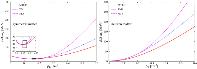
Fig. 1: The equation of states of three parameter sets for symmetric matter (left panel) and neutron matter (right panel). In both panels, the results of MTEC, TM1 and NL3 are corresponding the solid, the dotted and the dot-dashed lines, respectively. In the left panel, the open square indicates the empirical saturation point bib23 .

We treat the hadron phase by the RMF model. In the RMF model, the nucleon-nucleon interaction is mediated by scalar ($\varphi$), vector ($\omega$) and isovector ($\rho$) mesons. The Lagrangian of RMF model is written as

$$\mathcal{L}_{\textrm{RMF}}= \bar{\psi}(i\gamma^{\mu}\partial_{\mu}-m_{\textrm{N}}-g_{\varphi}\varphi-g_{\omega}\gamma^{\mu}\omega_{\mu}-g_{\rho}\gamma^{\mu}\rho^{a}_{\mu}\tau_{a})\psi$$

$$+\frac{1}{2}\partial^{\mu}\varphi\partial_{\mu}\varphi-\frac{1}{2}m^{2}_{\varphi}\varphi^{2}-\frac{1}{3}g_{2}\varphi^{3}-\frac{1}{4}g_{3}\varphi^{4}$$

$$-\frac{1}{4}\Omega^{\mu\nu}\Omega_{\mu\nu}+\frac{1}{2}m^{2}_{\omega}\omega^{\mu}\omega_{\mu}+\frac{1}{4}c_{3}(\omega^{\mu}\omega_{\mu})^{2}$$

$$-\frac{1}{4}R^{\mu\nu}_{a}R_{\mu\nu}^{a}+\frac{1}{2}m^{2}_{\rho}\rho^{\mu}_{a}\rho^{a}_{\mu},$$ (6)

where $\psi$ is the nucleon (N) field, and $\Omega^{\mu\nu}$ ($R^{\mu\nu}_{a}$) is the field strength of $\omega$ ($\rho$) meson. Masses of the particles are denoted by $m_{\rm N},m_{\varphi},m_{\omega},m_{\rho}$, Yukawa-coupling constants of nucleon with mesons are by $g_{\varphi},g_{\omega},g_{\rho}$ and self-interactions of $\varphi$ and $\omega$ mesons are by $g_{2},g_{3}$ and $c_{3}$. We take three RMF models of TM1 bib31 , NL3 bib32 and MTEC bib33 . The parameter sets of three models are summarized in TABLE 3, together with the saturation properties calculated by the models.

Under the mean field approximation, all the meson fields $\varphi$, $\omega$, $\rho$ are replaced by the mean values $\langle\varphi\rangle$, $\langle\omega^{0}\rangle\delta^{\mu 0}$, $\langle\rho^{0}_{3}\rangle\delta^{\mu 0}\delta_{a3}$, respectively. For simplicity, these mean values are denoted by $\varphi$, $\omega$, $\rho$. The mean values are determined by the Euler-Lagrange equations,

$$m^{2}_{\varphi}\varphi+g_{2}\varphi^{2}+g_{3}\varphi^{3}=-g_{\varphi}\rho_{\textrm{s}},$$ (7)

$$m^{2}_{\omega}\omega+c_{3}\omega^{3}=g_{\omega}\rho_{\rm B},$$ (8)

$$\rho=\frac{g_{\rho}}{m^{2}_{\rho}}\rho_{\rm I},$$ (9)

where $\rho_{\textrm{s}}$, $\rho_{\textrm{B}}$, $\rho_{\textrm{I}}$ are scalar, baryon-number and isospin densities.

The thermodynamic potential of the RMF model $\Omega_{\rm RMF}$ (per unit volume) is then obtained by

$$\Omega_{\rm RMF}=U_{\rm meson}-\frac{2}{\beta}\sum_{i=\textrm{p,n}}\int\frac{d^{3}\mathbf{p}}{(2\pi)^{3}}$$

$$\times\Bigl{[}\log(1+\textrm{e}^{-\beta(E-\tilde{\mu}_{i})})+\log(1+\textrm{e}^{-\beta(E+\tilde{\mu}_{i})})\Bigr{]},$$ (10)

where $E=\sqrt{\mathbf{p}^{2}+M^{2}_{\textrm{N}}}$ for the nucleon effective mass $M_{\textrm{N}}=m_{\textrm{N}}+g_{\varphi}\varphi$, and

$$U_{\rm meson}= \frac{1}{2}m^{2}_{\varphi}\varphi^{2}+\frac{1}{3}g_{2}\varphi^{3}+\frac{1}{4}g_{3}\varphi^{4}$$

$$-\frac{1}{2}m^{2}_{\omega}\omega^{2}-\frac{1}{4}c_{3}\omega^{4}-\frac{1}{2}m^{2}_{\rho}\rho^{2}$$

is the mesonic potential. The effective chemical potentials for neutron (n) and proton (p) are defined by $\tilde{\mu}_{\textrm{n,p}}=\mu_{\textrm{n,p}}-g_{\omega}\omega\pm g_{\rho}\rho$.

Figure. 1 shows the EoSs of symmetric matter (left panel) and neutron matter (right panel) calculated by TM1, NL3 and MTEC at $T=0$. As for densities smaller than the saturation point (open square), all the EoSs yield an universal line. On the other hand, there are remarkable differences among the EoSs for densities higher than the saturation point. MTEC EoS is softest, whereas NL3 EoS is stiffest. TM1 EoS lies halfway between them. The behavior of EoS in $\rho_{B}\gtrsim\rho_{0}$ largely affects the MR relation of NSs. Therefore, we can select which EoS model is preferable for the MR relation, particularly in $2M_{\rm sun}$ region.

II.3 TWO PHASE MODEL

In $\mu_{\rm q}/T=0$, it is established by LQCD simulations that the hadron-quark deconfinement transition is crossover bib39 . However, the pseudo-critical temperature is well estimated by the TPM bib21 . We thus use the TPM and the Gibbs criterion to determine the phase boundary of the hadron-quark phase transition for each set of $T$ and $\mu_{\textrm{B}}$.

Pressures of the EPNJL and the RMF models are obtained by

$$P_{\textrm{EPNJL}}(\mu_{\textrm{B}},T)=-(\Omega_{\textrm{EPNJL}}(\mu_{\textrm{B}},T)-\Omega_{\textrm{EPNJL}}(0,0))-B,$$ (11)

$$P_{\textrm{RMF}}(\mu_{\textrm{B}},T)=-\Omega_{\textrm{RMF}}(\mu_{\textrm{B}},T),$$ (12)

where the bag constant $B$ is introduced in $P_{\rm EPNJL}$ to describe the difference of vacuum between the hadron and quark phases. According to the Gibbs criterion, the quark phase (the hadron phase) takes place for the condition $P_{\textrm{EPNJL}}>P_{\textrm{RMF}}\ (P_{\textrm{EPNJL}}<P_{\textrm{RMF}})$. When $B$ is 100 $\textrm{MeV}^{4}$, our TPM can reproduce the LQCD prediction of $T_{\textrm{pc}}=171$ MeV of the deconfinement transition at $\mu_{\textrm{q}}/T=0$.

III RESULTS

We show our numerical results in this section. We first determine the value of $G_{\rm v4}(0)$ from LQCD data on the ratio $n_{\rm q}/n_{\rm SB}$ in the $\mu_{\rm q}/T=0$ limit bib4 ; bib11 . As for the RMF model, it is shown that MTEC and TM1 are proper EoSs, through the comparison with the NS observations bib27 ; bib28 ; bib29 .

Next, from the combinations of the two hadron-phase EoSs and EPNJL type (1)–(3), we construct TPMa1 - TPMa3, TPMb1 - TPMb3. In the TPMa3 and TPMb3, the density-dependent strength $G_{\rm v4}(n_{\rm q})$ of vector-type four-quark interaction is introduced. We parametrize the density dependence with a Gaussian form having a single parameter $b$, shown in Eq. (5). We determine the lower bound of $b$ assuming that the hadron-quark phase transition takes place in the core of NS. By using six models, the MR relation and the band of the hadron-quark phase transition line that allows the quark phase to exist in the core of NS are calculated.

III.1 DETERMINATION OF THE VALUE OF $G_{\rm v4}(0)$

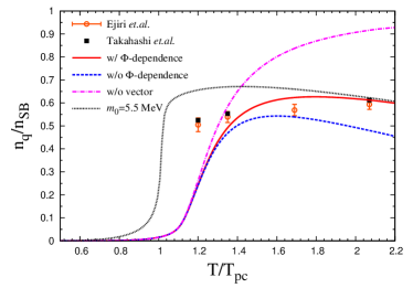
Fig. 2: Temperature dependence of $n_{\rm q}/n_{\rm SB}$ in the $\mu_{\rm q}/T=0$ limit. The temperature is normalized by the $T_{\rm pc}=171$ [MeV]. The data are the LQCD results bib4 ; bib11 . The lines are the results of calculations for the case with $\tilde{G}_{\rm v4}(0)$ (solid), $G_{\rm v4}(0)$ (dashed) and without vector-type four-quark interaction (dot-dashed). The dotted line corresponds to the results with $m_{0}=5.5$ MeV.

In the $T>T_{\rm pc}$ region, the chiral condensate $\sigma$ is nearly equal to zero, that is, the chiral symmetry is restored. Hence, the scalar-type four-quark interaction becomes negligible and only the vector-type four-quark interaction contributes to the ratio $n_{\rm q}/n_{\rm SB}$ that is $\mu_{\rm q}$-even and therefore finite even in the $\mu_{\rm q}/T=0$ limit. Thus, we determine the value $G_{\rm v4}(0)$ from LQCD data on $n_{\rm q}/n_{\rm SB}$ at $T>T_{\rm pc}$.

Figure 2 shows $T$ dependence of $n_{\rm q}/n_{\rm SB}$. Here, $T$ is normalized by $T_{\rm pc}=171$ MeV. In EPNJL model calculations, $m_{0}$ is taken to be 130 MeV, as already mentioned in Sec II. If the vector-type four-quark interaction is zero, the EPNJL model largely overestimates the LQCD data. Meanwhile, good agreement is seen for the case of $G_{\rm v4}(0)=0.36G_{\rm s4}$ at high $T$ such as $T=2T_{\rm pc}$. The comparison between the solid and dashed lines suggests that the entanglement coupling in $G_{\rm v4}(0)$ is necessary to reproduce the LQCD data. The result of $m_{0}=5.5$ MeV is also plotted. Comparing the dotted line with the solid line, we find that $m_{0}$ dependence is small at high $T$. This means that the value of $G_{\rm v4}(0)$ can be determined at high $T$ even if $m_{0}$ is heavier than physical value.

III.2 SELECTION OF RMF MODEL

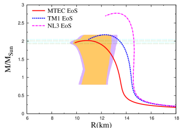
Fig. 3: The MR relation for three RMF EoSs. The two horizontal boxes are the $2M_{\rm sun}$ observational data bib27 ; bib28 . The two areas correspond to the 68% and 95% confidence counters estimated by Steiner et.al. bib29 .

Now, we select preferable RMF EoSs from the MR relation. The MR relation has one-to-one correspondence to the EoS through the Tolman-Oppenheimer-Volkov (TOV) equation bib40

$$\frac{dP}{dr}=-G\frac{M\epsilon}{r^{2}}\left(1+\frac{P}{\epsilon}\right)\left(1+\frac{4\pi Pr^{3}}{M}\right)\left(1-\frac{2GM}{r}\right)^{-1},$$

$$\frac{dM}{dr}=4\pi r^{2}\epsilon,$$

where $G$ is a gravitational constant and $\epsilon$ is an energy density. The NS has a crust region at low densities. As an EoS of the crust region, we use that of Miyatsu et.al. bib41 .

In solving the TOV equation, the electron and the muon should be taken into account to satisfy the charge neutral condition. We treat the electron as a massless free Fermion and the muon as a massive free Fermion. If the number densities, $n_{\textrm{e}}$ and $n_{\mu^{-}}$, of electron and muon are known, the charge neutral condition is given by

$$n_{\textrm{p}}=n_{\textrm{e}}+n_{\mu^{-}}$$ (13)

for the proton number density $n_{\rm p}$. In the inner of NS, the $\beta$-equilibrium condition is also satisfied:

$$\mu_{i}=b_{i}\mu_{\rm B}-q_{i}\mu_{\rm e}$$ (14)

for $i=$ p, n, e, $\mu^{-}$, where $b_{i}$ ($q_{i}$) is the baryon number (the electric charge) of particle $i$ and $\mu_{\textrm{e}}$ is the electron chemical potential. Solving the TOV equation numerically with the EoS that satisfies Eqs. (9) and (10), we can get the MR relation.

Figure. 3 illustrates the MR relation calculated by MTEC EoS, TM1 EoS and NL3 EoS. The data on MR relation in Fig. 3 are taken from Refs bib27 ; bib28 ; bib29 . The maximum mass $M_{\textrm{max}}$ and radius $R_{\rm max}$ is tabulated in TABLE 4. From Fig. 3, one can see that MTEC EoS is most consistent with all the data, particularly in the $2M_{\rm sun}$ region. TM1 EoS predicts a bit larger maximum radius, but it considerably well reproduce the data of MR relation. In NL3 EoS, the resulting $M_{\rm max}$ and $R_{\rm max}$ are inconsistent with the data of MR relation. We therefore take MTEC and TM1 EoSs as the hadron-phase EoS and construct the TPMa1–TPMa3, TPMb1–TPMb3.

Table 4: The maximum mass ($M_{\rm max}$) and radius ($R_{\rm max}$) predicted from three RMF models. The mass is normalized by the mass of sun $M_{\rm sun}$.

	MTEC	TM1	NL3
$M_{\textrm{max}}/M_{\rm sun}$	2.02	2.18	2.77
$R_{\textrm{max}}$ (km)	10.8	12.3	13.2

III.3 TRANSITON LINE OF TPMa1 AND TPMb1

We first consider the possibility of the hadron-quark phase transition in the core of NS by using TPMa1 and TPMb1. If the quark phase appears in the core of NS, Eqs. (9) and (10) should be also imposed on the quark-phase EoS:

$$\frac{2}{3}n_{\rm u}-\frac{1}{3}n_{\rm d}=n_{\rm e}+n_{\mu^{-}},$$

$$\mu_{\rm u}=\frac{1}{3}\mu_{\rm B}-\frac{2}{3}\mu_{\rm e},$$

$$\mu_{\rm d}=\frac{1}{3}\mu_{\rm B}+\frac{1}{3}\mu_{\rm e},$$

where $n_{\rm u}$ ($n_{\rm d}$) is the u-quark (d-quark) number density. Which phase is realized is determined from the Gibbs criterion.

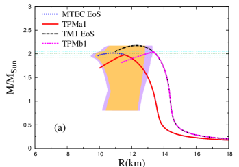
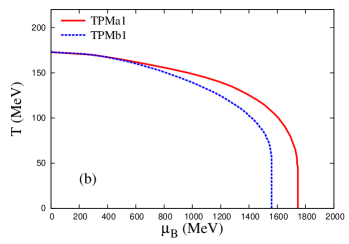
Fig. 4: The panel (a) shows the MR relation calculated from the TPMa1 (solid), TPMb1 (dashed), For comparison, the MR relation calculated from MTEC and TM1 EoSs are also plotted. In the panel (b), the hadron-quark phase transition lines for TPMa1 and TPMb1 are drawn.

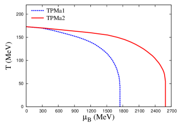
Fig. 5: The hadron-quark phase transition line for TPMa1 and TPMa2.

In Fig. 4, the panel (a) shows the MR relations calculated with TPMa1 and TPMb1. For comparison, the results calculated from MTEC and TM1 EoSs are plotted. In TPMa1, the quark phase appears at $M=1.97M_{\rm sun}$ before reaching $M_{\rm max}=2.02M_{\rm sun}$ and consistent with the data on MR relation. Also in TPMb1, the quark phase emerges at $M=2.04M_{\rm sun}$ before reaching $M_{\rm max}=2.17M_{\rm sun}$.

The panel (b) of Fig. 4 shows the hadron-quark phase transition line in the $T$-$\mu_{\rm B}$ plane for TPMa1 and TPMb1. The critical baryon chemical potential $\mu^{\rm c}_{\rm B}$ of the transition at $T=0$ is 1750 MeV for TPMa1 and 1560 MeV for TPMb1. If the $G_{\rm v4}(0)$ is positive, the quark-matter EoS becomes stiffer and thereby the predicted values of NS mass and $\mu^{\rm c}_{\rm B}$ are increasing. Therefore, TPMa1 and TPMb1 yield the lower bound of $\mu^{\rm c}_{\rm B}$ for each class of TPM for the quark phase to take place in the core of NS.

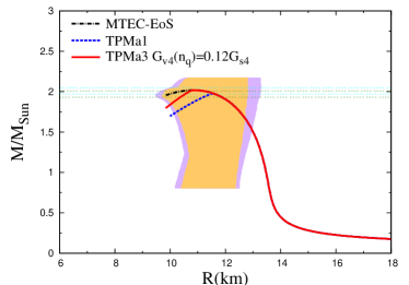
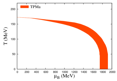
Fig. 6: (Left panel) The MR relation calculated from TPMa3. The results from TPMa1 and MTEC EoS are also plotted.
(Right panel) The band of the hadron-quark phase transition line. The upper (lower) bound of the band is calculated from TPMa3 (TPMa1). This region allows the quark phase appear in the core of NS.

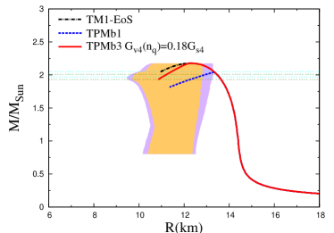
Fig. 7: (Left panel) The MR relation calculated from TPMb3. The results from TPMb1 and TM1 EoS are also plotted.
(Right panel) The band of the hadron-quark phase transition line. The upper (lower) bound of the band is calculated from TPMb3 (TPMb1). This region allows the quark phase appear in the core of NS.

III.4 TRANSITON LINE OF TPMa2 AND TPMb2

Next, we consider TPMa2 and TPMb2 with $G_{\rm v4}(0)=0.36G_{\rm s4}$. Figure. 5 illustrates the hadron-quark phase transition line for TPMa1 and TPMa2. One can see that the existence of $G_{\rm v4}(0)$ delays the transition toward higher $\mu_{\rm B}$. The value of $\mu^{\rm c}_{\rm B}$ for TPMa2 is 2600 MeV and the corresponding density is 13$\rho_{0}$. Such a density does not realize in the core of NS and hence the quark phase does not appear in the core of NS for TPMa2.

As for TPMb2, we find that the hadron-quark phase transition line does not reach the $\mu_{\rm B}$ axis. The reason is that the self interaction $(\omega^{\mu}\omega_{\mu})^{2}$ of $\omega$ meson more stabilizes the hadron phase with respect to increasing $\mu_{\rm B}$, while the vector-type four-quark interaction suppresses the appearance of quark phase. In fact, the quark phase is confirmed to never appear in the core of NS for TPMb2.

III.5 DENSITY DEPENDENCE OF $G_{\rm v4}$ AND TRANSITON LINE OF TPMa3 AND TPMb3

Finally, we consider TPMa3 and TPMb3. In TPMa3 and TPMb3, the quark phase is described by the EPNJL of type (3), that is, the strength of vector-type four-quark interaction depends on the quark number density $n_{\rm q}$ (See Eq. (5)). For TPMa3 (TPMb3), $\rho_{0}=0.153\ (0.145)\ \textrm{fm}^{-3}$ is used. The form Eq. (5) ensures that the interaction is invariant under the charge conjugation and $G_{\rm v4}(n_{\rm q})$ is positive for any $n_{\rm q}$. When $G_{\rm v4}(n_{\rm q})$ is negative, there is possibility that vector meson masses calculated with the random-phase-approximation becomes negative. Consequently, the $G_{\rm v4}(n_{\rm q})$ varies in a range $0\leq G_{\rm v4}(n_{\rm q})\leq G_{\rm v4}(0)=0.36G_{\rm s4}$. We discuss the lower bound of $b$ by assuming that the quark phase takes place in the core of NS.

The left panel of Fig. 6 shows the MR relation calculated with TPMa3. In TPMa3, the quark phase appears at $M_{\rm max}=2.02M_{\rm sun}$ and $n_{\rm q}=7.2\rho_{0}$, when the value of $G_{\rm v4}(n_{\rm q})$ is equal to $0.12G_{\rm s4}$. This means that $0.12G_{\rm s4}$ is the maximum value of $G_{\rm v4}(n_{\rm q})$ for the quark phase to appear in the core of NS. The corresponding value of $b$ is 0.001. The right panel of Fig. 6 illustrates the hadron-quark phase transition line. The lower bound of line is determined by the TPMa1 and upper bound is the TPMa3 with $b=0.001$. The values of $\mu^{\rm c}_{\rm B}$ lies in the $1750\textrm{MeV}\leq\mu^{\rm c}_{\rm B}\leq 1910$ MeV. If the value of $\mu^{\rm c}_{\rm B}$ exists in this region, the hadron-quark phase transition occurs in the core of NS. Note that the maximum value $\mu^{\rm c}_{\rm B}=1910$MeV is much smaller than $\mu^{\rm c}_{\rm B}=2600$MeV in TPMa2 shown in Fig. 5.

The left panel of Fig. 7 shows the MR relation calculated with TPMb3. As for TPMb3, the quark phase appears at $M_{\rm max}=2.17M_{\rm sun}$ and $n_{\rm q}=6\rho_{0}$, when the value of $G_{\rm v4}(n_{\rm q})$ is equal to $0.18G_{\rm s4}$, which is the maximum value of $G_{\rm v4}(n_{\rm q})$ for the quark phase appear in the core of NS in TPMb3. The corresponding value of $b$ is 0.001 and common between TPMa3 and TPMb3. The right panel of Fig. 7 illustrates the hadron-quark phase transition line. The lower bound of line is determined by the TPMb1 and upper bound is the TPMb3 with $b=0.001$. The values of $\mu^{\rm c}_{\rm B}$ lays in the $1560\textrm{MeV}\leq\mu^{\rm c}_{\rm B}\leq 1860$ MeV. The lower bound of $\mu_{\rm B}^{\rm c}$ is not same between TPMa1 and TPMb1, but upper value for TPMa3 and TPMb3 is nearly equal.

IV SUMMARY

In this paper, we constructed the TPM in which the EPNJL model is used in the quark phase and the RMF model is in the hadron phase. To make the TPM reasonable, we took LQCD data and NS observations as reliable constraints. For the quark-phase model, we determined the density-independent strength $G_{\rm v4}(0)$ of vector-type four-quark interaction from LQCD data on $n_{\rm q}/n_{\rm SB}$ in the $\mu_{\rm q}/T=0$ limit with small error bars. The obtained value is $G_{\rm v4}(0)=0.36G_{\rm s4}$ that is a bit larger than our previous work. For the hadron phase, we take three RMF models; NL3, TM1 and MTEC. We compared calculated MR relations with observed ones. We found that MTEC is most consistent with the data and TM1 is the second best, while NL3 is inconsistent.

We then take MTEC and TM1 for the hadron part of TPM and considered six types of TPMs (TPMa1–a3 and TPMb1–b3) that are combinations of the two types of hadron-phase EoS and EPNJL of type (1)–(3). For TPMa3 and TPMb3, we introduced the density-dependent strength $G_{\rm v4}(n_{\rm q})$ of vector-type four-quark interaction and assumed that the density-dependence is described as a Gaussian form having the single parameter $b$.

The MR relation and hadron-quark phase transition line are calculated for six TPMs. As a result, the hadron-quark phase transition occurs in the core of NS when $1750\textrm{MeV}\leq\mu^{\rm c}_{\rm B}\leq 1910$ MeV for TPMa and $1560\textrm{MeV}\leq\mu^{\rm c}_{\rm B}\leq 1850$ MeV for TPMb. For both TPMa and TPMb, the corresponding minimum value of $b$ is $b=0.001$.

- (1) K. Fukushima and T. Hatsuda, Rep. Prog. Phys. 74, 014001 (2011).
- (2) Z. Fodor, and S. D. Katz, Phys. Lett. B 534, 87 (2002).
- (3) C. R. Allton, S. Ejiri, S. J. Hands, O. Kaczmarek, F. Karsch, E. Laermann, Ch. Schmidt, and L. Scorzato, Phys. Rev. D 66, 074507 (2002).
- (4) S. Ejiri, Y. Maezawa, N. Ukita, S. Aoki, T. Hatsuda, N. Ishii, K. Kanaya, and T. Umeda, Phys. Rev. D 82, 014508 (2010).
- (5) P. de Forcrand and O. Philipsen, Nucl. Phys. B642, 290 (2002).
- (6) M. D’Elia and M. P. Lombardo, Phys. Rev. D 67, 014505 (2003).
- (7) M. D’Elia and F. Sanfilippo, Phys. Rev. D 80, 111501 (2009).
- (8) L. K. Wu, X. Q. Luo, and H. S. Chen, Phys. Rev. D76, 034505 (2007).
- (9) P. de Forcrand and O. Philipsen, Phys. Rev. Lett. 105, 152001 (2010).
- (10) J. Takahashi, K. Nagata, T. Saito, A. Nakamura, T. Sasaki, H. Kouno, and M. Yahiro Phys. Rev. D 88, 114504 (2013).
- (11) J. Takahashi, H. Kouno, and M. Yahiro, Phys. Rev. D 91, 014501 (2015).
- (12) Y. Sakai, T. Sasaki, H. Kouno, and M. Yahiro, Phys. Rev. D 82, 076003 (2010).
- (13) Y. Sakai, T. Sasaki, H. Kouno, and M. Yahiro, J. Phys. G: Nucl. Part. Phys. 39, 035004 (2012).
- (14) M. Ishii, T. Sasaki, K. Kashiwa, H. Kouno, and M. Yahiro, Phys. Rev. D 89, 071901(R) (2014).
- (15) M. Ishii, K. Yonemura, J. Takahashi, H. Kouno, and M. Yahiro, Phys. Rev. D 93, 016002 (2016).
- (16) T. Sasaki, N. Yasutake, M. Kohno, H. Kouno, and M. Yahiro, arXiv:1307.0681.
- (17) O. Lourenco, M. Dutra, A. Delfino, and M. Malheiro, Phys. Rev. D 84, 125034 (2011).
- (18) M. Kohno, Prog. Theor. Exp. Phys. 123, 02 (2015).
- (19) R. Brockmann and R. Machleidt, Phys. Rev. C 42, 1965 (1990).
- (20) A. Akmal, V. R. Pandharipande, and G. Ravenhall, Phys. Rev. C 58, 1804 (1998).
- (21) B. D. Serot and J. D. Walecka, Adv. Nucl. Phys. 16, 1 (1986).
- (22) P. B. Demorest, T. Pennucci, S. M. Ransom, M. S. E. Roberts, and J. W. T. Hessels, Nature (London) 467, 1081 (2010).
- (23) J. Antoniadis et.al., Science 340, 1233232 (2013).
- (24) A. W. Steiner, J. M. Lattimer, and E. F. Brown, Astrophys. J. 722, 33 (2010).
- (25) J. Sugano, J. Takahashi, M. Ishii, H. Kouno, and M. Yahiro, Phys. Rev. D 90, 037901 (2014).
- (26) K. Sumiyoshi, H. Kuwahara, and H. Toki, Nucl. Phys. A 581, 725 (1995).
- (27) G. A. Lalazissis, J. König, and P. Ring, Phys. Rev. C 55, 540 (1997).
- (28) T. Maruyama, T. Tatsumi, T. Endo, and S. Chiba, arXiv:0605075 (2006).
- (29) S. Rößner, C. Ratti, and W. Weise, Phys. Rev. D 75, 034007 (2007).
- (30) G. Boyd, J. Engels, F. Karsch, E. Laermann, C. Legeland, M. Lütgemeier, and B. Petersson, Nucl. Phys. B 496, 419 (1996).
- (31) W. Söldner, Proc. Sci. LAT2010 (2010) 215.
- (32) K. Kanaya, AIP Conf. Proc. 1343, 57 (2011); Proc. Sci., LAT2010 (2010) 012.
- (33) S. Borsányi, Z. Fodor, C. Hoelbling, S. D. Katz, S. Kreig, C. Ratti, and K. K. Szabo, J. High Energy Phys. 09. 073 (2010).
- (34) Y. Aoki, G. Endrödi, Z. Fodor, S. D. Katz and K. K. Szabó, Nature 443, 675 (2006).
- (35) S. L. Shapiro and S. A. Teukolsky, Black Holes, White Dwarfs and Neutron Stars, Wiley, New York (1983).
- (36) T. Miyatsu, S. Yamamuro, and K. Nakazato, Astrophys. J. 774, 4 (2013).