Tachyon warm-intermediate inflation in the light of Planck data

Abstract

We study the main properties of the warm tachyon inflation model in the framework of RSII braneworld based on Barrow’s solution for the scale factor of the universe. Within this framework we calculate analytically the basic slow roll parameters for different versions of warm inflation. We test the performance of this inflationary scenario against the latest observational data and we verify that the predicted spectral index and the tensor-to-scalar fluctuation ratio are in excellent agreement with those of Planck 2015. Finally, we find that the current predictions are consistent with those of viable inflationary models.

1 Introduction

Standard inflation driven by an inflaton field traces back to early efforts to alleviate the basic problems of the Big-Bang cosmology, namely horizon, flatness and monopoles Guth:1980zm ; Albrecht:1982wi . The nominal inflationary paradigm contains the slow-roll and the (P)reheating regimes. In the slow-roll phase the kinetic energy (which has the canonical form here) of the scalar field is negligible with respect to the potential energy $V(\phi)$ which implies a deSitter expansion of the Universe. However, after the slow-roll epoch the kinetic energy becomes comparable to the potential energy and thus the inflaton field oscillates around the minimum and progressively the universe is filled by radiation Shtanov:1994ce ; Kofman:1997yn .

Nevertheless, other theoretical patterns suggested a possible way to treat the physics of the early universe. For example, in the so-called warm inflationary scenario the radiation production occurs during the slow-roll epoch and the reheating period is avoided Berera:1995ie ; Berera:1996fm . The nature of the warm inflationary scenario is different with respect to that of the standard cold inflation. Warm inflation satisfies the condition $T>H$, where $T$ is the temperature and $H$ is the Hubble parameter, which implies that the fluctuations of the inflaton field are thermal instead of quantum. An obvious consequence of the above inequality is that in the case of warm inflation density perturbations arise from thermal fluctuations rather than quantum fluctuations Hall:2003zp ; Moss:1985wn ; Berera:1999ws . Specifically, thermal fluctuations are produced during the warm inflationary epoch and they play a central role toward describing the CMB anisotropies and thus providing the initial seeds for the formation of large scale structures. Of course, after this epoch the universe enters in the radiation dominated phase as it should Berera:1995ie ; Berera:1996fm . In order to achieve warm inflation one may use a tachyon scalar field for which the kinetic term does not follow the canonical form (k-inflation ArmendarizPicon:1999rj ). It has been found that tachyon fields which are associated with unstable D-branes Sen:2002nu can be responsible for the cosmic acceleration in early times Sen:2002an ; Sami:2002fs ; ArmendarizPicon:1999rj .

Notice, that tachyon potentials have the following two properties: the maximum of the potential occurs when $\phi\rightarrow 0$ while the corresponding minimum takes place when $\phi\rightarrow\infty$. From the dynamical viewpoint one may obtain the equations of motion using a special Lagrangian Gibbons:2002md which is non-minimally coupled to gravity:

$$L=\sqrt{-g}\left[\frac{R}{16\pi G}-V(\phi)\sqrt{1-g^{\mu\nu}\partial_{\mu}\phi\partial_{\nu}\phi}\right]\;.$$ (1)

Considering a spatially flat Friedmann-Robertson-Walker (hereafter FRW) space-time the stress-energy tensor is given by

$$T^{\mu}_{\nu}=\frac{\partial L}{\partial(\partial_{\mu}\phi)}\partial_{\nu}\phi-g^{\mu}_{\nu}L={\rm diag}(-\rho_{\phi},p_{\phi},p_{\phi},p_{\phi})$$ (2)

equation where $\rho_{\phi}$ and $p_{\phi}$ are the energy density and pressure of the scalar field. Combining the above set of equations one can derive

$$\rho_{\phi}=\frac{V(\phi)}{\sqrt{1-\dot{\phi}^{2}}}$$ (3)

and

$$P_{\phi}=-V(\phi)\sqrt{1-\dot{\phi}^{2}}$$ (4)

Where $\phi$ is tachyon scalar field in unite of inverse Planck mass $M_{pl}^{-1}$, and $V(\phi)$ is potential associated with the tachyon field. In the past few years, there was an intense debate among cosmologists and particle physicists regarding those phenomenological models which can be produced in extra dimensions. For example, the reduction of higher-dimensional gravitational scale, down to TeV-scale, could be presented by an extra dimensional scenario ArkaniHamed:1998rs ; ArkaniHamed:1998nn ; Antoniadis:1998ig . In these scenarios, gravity field propagates in the bulk while standard models of particles are confined to the lower-dimensional brane. In this framework, the extra dimension induces additional terms in the first Friedmann equation Binetruy:1999ut ; Binetruy:1999hy ; Shiromizu:1999wj . Especially, if we consider a quadratic term in the energy density then we can extract an accelerated expansion of the early universe Maartens:1999hf ; Cline:1999ts ; Csaki:1999jh ; Ida:1999ui ; Mohapatra:2000cm . In the current study we consider the tachyon warm inflation model in the framework of Randall-Sundrum II braneworld which contains a single, positive tension brane and a non-compact extra dimension.

Following the lines of Ref.Herrera:2015aja , we attempt to study the main properties of the warm inflation in which the scale factor evolves as $a(t)\propto\exp(At^{f})$, where $0<f<1$ ("intermediate inflation"). In this case cosmic expansion evolves faster than the power-law inflation ($a\propto t^{p}$, $p>1$) and slower than the standard deSitter one, $a(t)\propto{\rm exp}(H_{I}t)$ [$H(t)=H_{I}=$const.]. More details regarding the cosmic expansion in various inflationary solutions can be found in the paper of Barrow Barrow:1996bd .

In the current work, we investigate the possibility of using the intermediate solution in the case of warm tachyon inflation. Specifically, the structure of the article is as follows: In section II we briefly discuss the main properties of the warm inflation, while in section III we provide the slow roll parameters. In section IV we study the performance of our predictions against the Planck 2015 data. Finally, the main conclusions are presented in section VI.

2 Tachyon warm inflation

Let us assume a flat, homogeneous and isotropic Friedmann-Robertson-Walker (FRW) universe, in which the radiation era is endowed with the scalar field described by the Lagrangian (1) in the context of the Randall-Sundrum II (RSII) brane Randall:1999vf . Following the notations of Shiromizu:1999wj ; Binetruy:1999ut ; Binetruy:1999hy ; Berera:1995ie ; Berera:1996fm ; Herrera:2015aja one may check that the basic cosmological equations are

$$H^{2}=\frac{8\pi}{3M_{pl}^{2}}\rho(1+\frac{\rho}{2\lambda})$$ (5)

equation

$${\dot{\rho}}_{\phi}+3H(\rho_{\phi}+p_{\phi})=-\Gamma{\dot{\phi}}^{2}$$ (6)

$${\dot{\rho}}_{\gamma}+3H(\rho_{\gamma}+p_{\gamma})=\Gamma{\dot{\phi}}^{2}$$ (7)

where $\Gamma$ is the dissipation coefficient, in unit of $M_{pl}^{5}$. The latter two equations (6),(7) imply the continuity equation, namely ${\dot{\rho}}+3H(\rho+p)=0$. Notice, that Eqs.(6) and (7) have been proposed by various authors such as Cai:2010wt ; Herrera:2006ck ; delCampo:2008fc ; Setare:2012fg ; Setare:2013dd ; Zhang:2013waa . In these studies the quantity $\Gamma\dot{\phi}^{2}$ is the dissipation term which is introduced phenomenologically in order to describe the nearly-thermal radiation bath that is the outcome of the warm inflationary scenario. It is well known that Tachyon inflation in its standard picture (cold inflation) suffers from a serious problem. In particular, reheating and matter creation are both problematic because the tachyon fields in such theories do not oscillate around the minimum of the potential Kofman:2002rh . This problem can be alleviated in the context of warm inflation. In this scenario radiation production occurs during the slow-roll era which implies that reheating is avoided and thus the universe heats up and finally it enters in the radiation era Berera:1995ie (See Eqs.(6) and (7)).

In the above set of equations, an over-dot denotes derivative with respect to time, $\rho=\rho_{\phi}+\rho_{\gamma}$ and $p=p_{\phi}+p_{\gamma}$ ($p_{\gamma}=\rho_{\gamma}/3$) are the total density and pressure, $\rho_{\phi}$ and $\rho_{\gamma}$ are the scalar field and radiation densities, $H={\dot{a}}/a$ is the Hubble parameter. Notice, that $\lambda$ is the brane tension which obeys the following restriction $\lambda\geq(10TeV)^{4}$ Cline:1999ts ; Brax:2003fv ; Clifton:2011jh . Obviously, substituting equations (3),(4) in Eq.(6) it is easy to derive the modified Klein-Gordon equation which describes the time evolution of the tachyon field. This is

$$\frac{\ddot{\phi}}{1-\dot{\phi}^{2}}+3H\dot{\phi}+\frac{V^{\prime}}{V}=-\frac{\Gamma}{V}\dot{\phi}\sqrt{1-\dot{\phi}^{2}}\;,$$ (8)

where $V^{\prime}(\phi)=dV/d\phi$.

The above cosmological equations imply that the model is strongly affected by the quantity $\Gamma$. This is due to the fact that radiation is exchanging energy with the tachyon field and this is reflected in the corresponding behavior of dissipation coefficient $\Gamma$, which is negligible in the classical inflationary paradigm by definition. Although, the precise functional form of $\Gamma$ is still an open issue, a number of different parametrizations have been proposed in the literature treating the functional form of $\Gamma$ (see Hall:2003zp ; BasteroGil:2012cm ; Bastero-Gil:2014oga ; Bartrum:2013fia ). In the current work we use the well known parametrization of

$$\Gamma=\Gamma_{c}\phi^{b}T^{c}\;,$$ (9)

where $T$ is the temperature and $\Gamma_{c}$ is constant.

During the warm inflationary epoch, the energy density of the scalar field dominates the total fluid (stable regime BasteroGil:2012zr ) and thus Eq.(5) becomes

$$H^{2}=\frac{8\pi}{3M_{pl}^{2}}\rho_{\phi}(1+\frac{\rho_{\phi}}{2\lambda})$$ (10)

or

$$H^{2}=\frac{8\pi}{3M_{pl}^{2}}\frac{V(\phi)}{\sqrt{1-\dot{\phi}^{2}}}\left(1+\frac{V(\phi)}{2\lambda\sqrt{1-\dot{\phi}^{2}}}\right)\;.$$ (11)

Another important quantity in this kind of studies is the dimensionless dissipation parameter which characterizes the type of inflation and it is defined as (for more details see appendix)

$$R=\frac{\Gamma}{3H\rho_{\phi}}.$$ (12)

The above definition is presented for warm tachyon inflation in several papers Herrera:2006ck ; Setare:2012fg ; Setare:2013ula ; Setare:2014gya ; Setare:2014uja ; Setare:2013dd . Notice, that for the canonical scalar field model of warm inflation, the corresponding dimensionless ratio is defined as $\frac{\Gamma}{3H}$.

In the weak dissipation regime, the ratio $R$ tends to zero ($\Gamma/3H\rho_{\phi}\ll 1$), however, in the strong dissipation regime, the coefficient $\Gamma$ guides the damped evolution of the scalar field. Now using Eq.(8) and Eq.(11) in the high-dissipation regime ($\Gamma\gg 3H\rho_{\phi}$) to prove that

$$\dot{\phi}^{2}=-\frac{3M_{pl}^{2}}{4\pi}\frac{(H\dot{H})}{\Gamma}\left(1+\frac{3M_{pl}^{2}H^{2}}{4\pi\lambda}\right)^{-\frac{1}{2}}\;.$$ (13)

Owing to the fact that during inflation the parameters $H$, $\Gamma$ and $\phi$ are slowly varying functions the production of radiation become quasi-stable when $\dot{\rho}\ll 4H\rho_{\gamma},$ and $\dot{\rho}_{\gamma}\ll\Gamma\dot{\phi}^{2}$ (Berera:1995ie, ; Berera:1996fm, ; Hall:2003zp, ). Under these conditions, using Eqs.(8) and (13) we write the radiation density as follows:

$$\rho_{\gamma}=\frac{\Gamma\dot{\phi}^{2}}{4H}=-\frac{3M_{pl}^{2}\dot{H}}{16\pi}\left(1+\frac{3M_{pl}^{2}H^{2}}{4\pi\lambda}\right)^{-\frac{1}{2}}\;.$$ (14)

The latter formula can be identified with the equation relating $\rho_{\gamma}$ with the radiation temperature $T$. Indeed, under of adiabatic condition we may write

$$\rho_{\gamma}=C_{\gamma}T^{4}$$ (15)

where $C_{\gamma}=\frac{\pi^{2}g_{*}}{30}$ and $g_{*}$ is the degrees of freedom of the created massless modes (Kolb1990, ). Combining Eq.(14) and (15) we obtain the temperature

$$T=\left(-\frac{3M_{pl}^{2}\dot{H}}{16\pi C_{\gamma}}\right)^{\frac{1}{4}}\left(1+\frac{3M_{pl}^{2}H^{2}}{4\pi\lambda}\right)^{-\frac{1}{8}}\;.$$ (16)

Lastly, with the aid of Eqs.(11) and (14) we obtain the potential of the scalar field

$$V=\lambda\left[-1+\left(1+\frac{3M_{pl}^{2}H^{2}}{4\pi\lambda}\right)^{\frac{1}{2}}\right]$$ (17)

$$\times\left(1+\frac{3M_{pl}^{2}}{4\pi}\frac{(H\dot{H})}{\Gamma}\left[1+\frac{3M_{pl}^{2}H^{2}}{4\pi\lambda}\right]^{-\frac{1}{2}}\right)^{\frac{1}{2}}\;.$$

3 Slow-roll parameters

Let us present here the main quantities of the tachyonic inflation. In particular, the basic slow-roll parameters are given by

$$\epsilon=-\frac{\dot{H}}{H^{2}}$$ (18)

equation

$$\eta=-\frac{\ddot{H}}{2H\dot{H}}\;.$$ (19)

equation In this context, the number of e-folds is written as

$$N=\int_{t}^{t_{end}}Hdt$$ (20)

equation where $t_{end}$ is the value of the cosmic time at the end of inflation, namely $\epsilon(\phi_{end})\simeq 1$ where $\phi_{end}=\phi(t_{end})$.

Also, the power spectrum of the scalar fluctuations is given by (Berera:1995ie, ; Berera:1996fm, )

$$P_{s}=\frac{H^{2}}{\dot{\phi}^{2}}\delta\phi^{2}\;.$$ (21)

equation An important feature of the warm inflationary model is related with the fact that the origin of $\delta\phi$ is thermal and not quantum as we consider in the nominal inflationary paradigm. In the case of warm inflation it has been found (Berera:1995ie, ; Berera:1996fm, ; Hall:2003zp, ) that scalar perturbations are written as

$$\delta\phi^{2}\simeq\frac{k_{F}T}{2M_{pl}^{4}\pi^{2}}\;,$$ (22)

where the wave number $k_{F}=\sqrt{\frac{\Gamma H}{V}}=H\sqrt{\frac{\Gamma}{3HV}}\geq H$ corresponds to the freeze-out scale at the special point when, the dissipation damps out to thermally excited fluctuations of inflaton ($\frac{V^{\prime\prime}}{V^{\prime}}<\frac{\Gamma H}{V}$) Taylor:2000ze . Notice, that Eq.(22) is valid in the high-dissipation regime $R\gg 1$. As we have already mentioned in the previous section we study our model via Eq.(13) in the context of high-dissipation regime, which means that for scalar perturbations we can utilize Eq.(22).

Inserting the freeze-out wave-number and Eq.(22) into Eq.(21) we find after some simple calculations that the power spectrum of the tachyonic scalar field is given by

$$P_{s}\simeq\frac{H^{\frac{5}{2}}\Gamma^{\frac{1}{2}}T}{2\pi^{2}M_{pl}^{4}V^{\frac{1}{2}}\dot{\phi}^{2}}\;.$$ (23)

We would like to point out that in the case of canonical scalar fields within the framework of warm inflation one can find other forms of the power spectrum $P_{s}$ in Refs.(Bartrum:2013fia, ; Ramos:2013nsa, ; Bastero-Gil:2014jsa, ). The corresponding spectral index $n_{s}$ is defined in terms of the $P_{s}$ slow-roll parameters, as usual LL , by

$$n_{s}-1=\frac{d\ln P_{s}}{d\ln k}\;.$$ (24)

On the other hand, it has been found Langlois:2000ns that the power spectrum of the tensor perturbations which are defined on the brane takes the form

$$P_{t}=\frac{64\pi}{M_{pl}^{2}}\left(\frac{H}{2\pi}\right)^{2}G^{2}(x)$$ (25)

where $x\equiv\left[\frac{3HM_{pl}^{2}}{4\pi\lambda}\right]^{\frac{1}{2}}$ and $G(x)=[\sqrt{1+x^{2}}-x^{2}\sinh^{-1}(\frac{1}{x})]^{-\frac{1}{2}}$ arises from normalization of zero-mod of a graviton Langlois:2000ns . Therefore, using the so called tensor-to-scalar ratio we arrive at

$$r=32\pi M_{pl}^{2}\frac{V^{\frac{1}{2}}\dot{\phi}^{2}}{H^{\frac{1}{2}}\Gamma^{\frac{1}{2}}T}G^{2}(x)\;.$$ (26)

In order to proceed with the analysis it would help to know the functional form of the scale factor $a(t)$. Barrow Barrow:1996bd showed that under of specific conditions we can have an intermediate inflation in which the scale factor satisfies the following exponential form:

$$a(t)=a_{I}\exp(At^{f})\;,$$ (27)

which provides

$$H(t)=\frac{{\dot{a}}(t)}{a(t)}=Aft^{f-1}\;,$$ (28)

where $f$ satisfies the restriction $0<f<1$. The above expansion evolves faster than the power-law inflation ($a\propto t^{p}$, $p>1$) and slower than the standard deSitter one, $a(t)\propto{\rm exp}(H_{I}t)$ [$H(t)=H_{I}=$const.]. Considering the functional form (9), one has to deal in general with the following four parametrizations, which have been considered within different approaches in the literature. Depending on the values of $(b,c)$ we have: (I)- the situation in which the formula is $\Gamma=\Gamma_{3}T^{3}\phi^{-2}$, $(b,c)=(3,-2)$. The constant parameter $\Gamma_{3}$ corresponds to $0.02h^{2}\mathcal{N}_{Y}$ where there is generic supersymmetric (SUSY) model with chiral superfields $X$, $\Phi$ and $Y_{i}=1,...\mathcal{N}_{Y}$. This case is mostly used in the low temperature regime where $m_{\chi}$ ($m_{\chi}$ is the mass of catalyst field) (Bastero-Gil:2014oga, ; Bastero-Gil:2013nja, ); (II)- for $(b,c)=(2,-1)$ we have $\Gamma=\Gamma_{2}\phi^{2}T^{-1}$. This parametrization has been used for non-SUSY models Berera:1998gx ; Yokoyama:1998ju . Q5: (III)- the case where $\Gamma=\Gamma_{0}$ is a positive constant (hereafter $\Gamma_{0}$-parametrization: see Herrera:2006ck ; Deshamukhya:2009wc ; Setare:2012fg ; Setare:2013ula ; Setare:2013qfa ; Setare:2014gya ; Setare:2014uja ; Setare:2015cta ; Setare:2013dd ) which implies that the pair $(b,c)$ in Eq.(9) is strictly equal to $(0,0)$ and finally (IV) we utilize the so called high temperature regime (hereafter $\Gamma_{1}$-parametrization) in which we select $(b,c)=(0,1)$ and thus $\Gamma\propto T$ (see also Panotopoulos:2015qwa ). In this paper, we are going to focus on parameterizations (III) and (IV) in order to calculate the slow roll parameters. Lastly, we remind the reader that in the framework of warm inflationary model thermal fluctuations dominate over the quantum fluctuations.

Combining the latter argument with the fact that thermal fluctuations are proportional to temperature $T$ while quantum fluctuations are proportional to $H$, one can easily derive the condition $T>H$. Obviously, if we consider our model in the high temperature regime ($\Gamma\propto T$) then the aforesaid restriction ($T>H$) is satisfied. For more details we refer the reader the work of Panotopoulos:2015qwa .

3.1 $\Gamma_{0}$-parametrization

In this inflationary scenario ($\Gamma=\Gamma_{0}$=const.) with the aid of Eq.(28) we integrate Eq.(13) and we obtain the evolution of the scalar field in terms of the hyper-geometric function Arfken ; Abramowitz

$$\phi(t)-\phi_{0}=\frac{F(t)}{K}$$ (29)

where

$$F(t) = t^{\frac{2f-1}{2}}\times$$

$${}_{2}F_{1} \left[\frac{1}{4},\frac{1-2f}{4(1-f)},\frac{5-6f}{4(1-f)},-\frac{3M_{pl}^{2}f^{2}A^{2}t^{2f-2}}{4\pi\lambda}\right]\;,$$

$$K=-\left(\frac{16\pi\Gamma_{0}(1-f)}{3M_{pl}^{2}f^{2}A^{2}}\right)^{\frac{1}{2}}\frac{\Gamma(\frac{5-6f}{4(1-f)})}{\Gamma(\frac{1-2f}{4(1-f)})}$$

and $\Gamma(n)$ is the normal Gamma-function. Notice, that without losing the generality we have set $\phi_{0}=0$.

Now we can derive the Hubble parameter $H$ and the associated potential $V(\phi)$ in the limit of $\dot{\phi}^{2}\ll V(\phi)$

$$H(\phi)=fA(F^{-1}[K\phi])^{f-1}$$ (31)

$$V(\phi)\simeq\lambda(-1+\sqrt{1+\frac{3M_{pl}^{2}f^{2}A^{2}[F^{-1}(K\phi)]^{2f-2}}{4\pi\lambda}})$$

where $F^{-1}(\phi)$ is the inverse function of $F(t)$. Clearly, if we substitute Eq.(31) in the slow-roll parameters then we have

$$\epsilon=\frac{(1-f)t^{-f}}{fA}=\frac{1-f}{fA[F^{-1}(K\phi)]^{f}}$$ (32)

$$\eta=\frac{(2-f)t^{-f}}{2fA}=\frac{2-f}{2fA[F^{-1}(K\phi)]^{f}}\;.$$ (33)

Notice, that in order to extract the latter equalities in Eqs(32), (33) we used Eqs.(28), (29). In our warm intermediate case the condition $\epsilon=1$, insures the beginning of inflation Barrow:2006dh ; Barrow:1993zq . Therefore, utilizing Eq.(20), we can derive the number of e-folds

$$N=\int_{t_{in}}^{t_{*}}Hdt=A(t_{*}^{f}-t_{in}^{f})$$

$$=A\left([F^{-1}(K\phi)]^{f}-[F^{-1}(K\phi_{in})]^{f}\right) \;.$$

Plugging $\phi_{in}$ into Eq.(32) and using the constraint $\epsilon(\phi_{in})\simeq 1$ we find

$$\phi_{in}=\frac{1}{K}F(y),\;\;\;\;\;y=\left(\frac{1-f}{fA}\right)^{\frac{1}{f}}\;.$$ (35)

In order to proceed with the analysis we need to know the values of $N$ and $\phi_{in}$. Firstly, it is natural to consider that the number of e-folds is 50 or 60. Secondly, using the condition $\epsilon(\phi_{in})=1$ and Eqs. (3.1), (• ‣ 4) we can estimate the slow-roll parameters.

Now we focus on the power spectrum formulas. Specifically, inserting the appropriate expressions into Eq.(23) we define the scalar power spectrum

$$P_{s}=p_{1}I(N)^{\frac{3f}{4}}\left[-1+\left(1+\frac{3M_{pl}^{2}f^{2}A^{2}}{4\pi\lambda I(N)^{2-2f}}\right)^{\frac{1}{2}}\right]^{-\frac{1}{2}}$$ (36)

$$\times\left(1+\frac{3M_{pl}^{2}f^{2}A^{2}}{4\pi\lambda I(N)^{2-2f}}\right)^{\frac{3}{8}}$$

where $p_{1}=(\frac{\Gamma_{0}^{6}f^{3}A^{3}}{3^{3}M_{pl}^{6}\pi^{5}(1-f)^{3}C_{\gamma}})^{\frac{1}{4}}$ and $I(N)=\left[\frac{1+f(N-1)}{fA}\right]^{\frac{1}{f}}$. Combining the definition of the spectral index $n_{s}$ (24) and the above equation we obtain

$$n_{s}-1=-\frac{3}{4A}I(N)^{-f}+n_{1}+n_{2}$$ (37)

where in the derivation of the above equality we have used

$$n_{1}=\frac{3M_{pl}^{4}(f-1)fA}{8\pi\lambda}I(N)^{f-2}\left(1+\frac{3M_{pl}^{2}f^{2}A^{2}}{4\pi\lambda I(N)^{2-2f}}\right)^{-\frac{1}{2}}$$ (38)

$$\times\left[-1+(1+\frac{3M_{pl}^{2}f^{2}A^{2}}{4\pi\lambda I(N)^{2-2f}})^{\frac{1}{2}}\right]^{-1}$$

$$n_{2}=\frac{9M_{pl}^{2}(1-f)fA}{16\pi\lambda}I(N)^{f-2}\left(1+\frac{3M_{pl}^{2}f^{2}A^{2}}{4\pi\lambda I(N)^{2-2f}}\right)^{-1}\;.$$

Lastly, based on Eq.(26) we compute the tensor-to-scalar ratio parameter

$$r=r_{1}I(N)^{\frac{5f-8}{4}}\left(1+\frac{3M_{pl}^{2}f^{2}A^{2}}{4\pi\lambda I(N)^{2-2f}}\right)^{-\frac{3}{8}}$$ (39)

$$\left[-1+\left(1+\frac{3M_{pl}^{2}f^{2}A^{2}}{4\pi\lambda I(N)^{2-2f}}\right)^{\frac{1}{2}}\right]^{\frac{1}{2}}G^{2}(N)$$

where $r_{1}=(\frac{2^{16}\lambda^{2}3^{3}C_{\gamma}\pi(fA)^{5}(1-f)^{3}}{M_{pl}^{2}\Gamma_{0}^{6}})^{\frac{1}{4}}$.

3.2 $\Gamma_{1}$-parametrization

Using the same methodology as in the previous section we provide the basic slow-roll parameters in the case of $\Gamma_{1}$-parametrization, namely $\Gamma=\Gamma_{1}T$, where $\Gamma_{1}$ is constant. In particular, from Eqs.(28,13) the tachyon field is written as

$$\phi-\phi_{0}=\frac{{\tilde{F}}(t)}{\tilde{K}}$$ (40)

where ${\tilde{F}}(t)$ and $\tilde{K}$ are given by the following expressions

$${\tilde{F}}(t)=t^{\frac{7f-2}{8}}\times$$ (41)

$${}_{2}F_{1}\left[\frac{3}{16},\frac{7f-2}{16(f-1)},\frac{23f-18}{16(f-1)},-\frac{3M_{pl}^{2}f^{2}A^{2}}{4\pi\lambda}t^{2f-2}\right]$$

$$\tilde{K}=-\left(\frac{2^{6}\pi\Gamma_{1}^{4}(1-f)^{5}}{3M_{pl}^{2}C_{\gamma}f^{7}A^{7}}\right)^{\frac{1}{8}}\frac{\Gamma(\frac{23f-18}{16(f-1)})}{\Gamma(\frac{7f-2}{16(f-1)})}\;.$$

Also here we have set $\phi_{0}=0$.

Now the Hubble parameter, the potential and the corresponding slow-roll parameters are given by

$$H(\phi)=fA({\tilde{F}}^{-1}[{\tilde{K}}\phi])^{f-1}$$ (42)

$$V(\phi)\simeq\lambda(-1+\sqrt{1+\frac{3M_{pl}^{2}f^{2}A^{2}[{\tilde{F}}^{-1}({\tilde{K}}\phi)]^{2f-2}}{4\pi\lambda}})$$

$$\epsilon=\frac{1-f}{fA[{\tilde{F}}^{-1}({\tilde{K}}\phi)]^{f}}\;,$$ (43)

$$\eta=\frac{2-f}{2fA[{\tilde{F}}^{-1}({\tilde{K}}\phi)]^{f}}\;.$$ (44)

where ${\tilde{F}}^{-1}(K\phi)$ is inverse function of ${\tilde{F}}(t)$. In the current case the number of e-folds becomes

$$N=\int_{t_{in}}^{t_{*}}Hdt=A(t_{*}^{f}-t_{in}^{f})$$

$$=A\left([{\tilde{F}}^{-1}({\tilde{K}}\phi)]^{f}-[{\tilde{F}}^{-1}({\tilde{K}}\phi_{in})]^{f}\right) \;.$$

and following standard lines the end of inflation takes place when

$$\phi_{in}=\frac{1}{\tilde{K}}\tilde{F}(y),\;\;\;\;\;\;y=\left(\frac{1-f}{fA}\right)^{\frac{1}{f}}\;.$$ (46)

The scalar power-spectrum can be easily identified by comparing the current cosmological expressions with Eq.(23), and we find

$$P_{s}=p_{2}I(N)^{\frac{9f-6}{8f}}\left[-1+\left(1+\frac{3M_{pl}^{2}f^{2}A^{2}}{4\pi\lambda I(N)^{2-2f}}\right)^{\frac{1}{2}}\right]^{-\frac{1}{2}}$$ (47)

$$\times\left[1+\frac{3M_{pl}^{2}f^{2}A^{2}}{4\pi\lambda I(N)^{2-2f}}\right]^{\frac{3}{16}}$$

where $p_{2}=\frac{2(\Gamma_{1}fA)^{\frac{3}{2}}}{3M_{pl}^{2}\lambda^{\frac{1}{2}}}(\frac{16\pi C_{\gamma}}{3M_{pl}^{2}(1-f)})^{\frac{3}{8}}$. If we take the aforementioned $P_{s}$ formula we find the following spectral index

$$n_{s}-1=-\frac{9f-6}{8fA}I(N)^{-f}+n_{1}+n_{2}$$ (48)

where

$$n_{1}=\frac{3M_{pl}^{4}(f-1)fA}{8\pi\lambda}I(N)^{f-2}\left(1+\frac{3M_{pl}^{2}f^{2}A^{2}}{4\pi\lambda I(N)^{2-2f}}\right)^{-\frac{1}{2}}$$ (49)

$$\times\left[-1+(1+\frac{3M_{pl}^{2}f^{2}A^{2}}{4\pi\lambda I(N)^{2-2f}})^{\frac{1}{2}}\right]^{-1}$$

$$n_{2}=\frac{9M_{pl}^{2}(1-f)fA}{32\pi\lambda}I(N)^{f-2}\left(1+\frac{3M_{pl}^{2}f^{2}A^{2}}{4\pi\lambda I(N)^{2-2f}}\right)^{-1}$$

Finally, the tensor-to-scalar ratio [see Eq.26)] takes the form

$$r=r_{2}I(N)^{\frac{7f-6}{8}}\left(1+\frac{3M_{pl}^{2}f^{2}A^{2}}{4\pi\lambda I(N)^{2-2f}}\right)^{\frac{-3}{16}}$$ (50)

$$\left[-1+(1+\frac{3M_{pl}^{2}f^{2}A^{2}}{4\pi\lambda I(N)^{2-2f}})^{\frac{1}{2}}\right]^{\frac{1}{2}}G^{2}(N)$$

where $r_{2}=\frac{24\lambda^{\frac{1}{2}}(fA)^{\frac{7}{8}}}{\Gamma_{1}^{\frac{3}{2}}}\left(\frac{16\pi C_{\gamma}(1-f)}{3M_{pl}^{2}}\right)^{\frac{3}{8}}$.

4 Comparison with observation

The analysis of Planck Ade:2015lrj and BICEP2/Keck Array joint data sets has provided a new constraint on inflationary scenarios Martin:2013tda . In particular, the comprehensive analysis of Planck data Ade:2015lrj indicates that single scalar-field models of slow-roll inflation have a very low tensor-to-scalar fluctuation ratio $r=P_{t}/P_{s}\ll 1$, a scalar spectral index $n_{s}=0.968\pm 0.006$ and no appreciable running. The upper bound set by the Planck team and the joint analysis of BICEP2/Keck Array/Planck joint on tensor-to-scalar fluctuation ratio is $r<0.11$. In this section we attempt to test the performance of the warm inflationary model against the above observational results.

Let us now concentrate on our results. Notice, that in the case of warm inflation the number of degrees of freedom becomes $g_{*}\simeq 200$ ($C_{\gamma}\simeq 70$,BasteroGil:2006vr ) Also, for the rest of the paper we have set $\lambda=10^{-14}$. Concerning the number of e-folds, it is natural to consider that $N$ lies in the interval $[50,60]$. Here, we have set it either to 50 or 60. In figures 1 ($\Gamma_{0}$ parametrization) and 2 ($\Gamma_{1}$ parametrization) we present the $A-f$ allowed region in which our $(n_{s},r)$ results satisfy the above restrictions of Planck within 1$\sigma$ uncertainties. In the case of $\Gamma_{0}$ model, we observe that for various values of the dissipation coefficient there is a narrow region in the $A-f$ plane which is consistent with the observed values of $n_{s}$ and $r$. The absence of $A-f$ pair solutions and thus of $(n_{s},r)$, appear for $\Gamma_{0}\leq 10^{-10}$.

For the $\Gamma_{1}$ parametrization the situation is slightly different. Figure (2) shows broader $A-f$ regions with respect to those of $\Gamma_{0}$ parametrization. Also in this case we verify that for $\Gamma_{1}\leq 10^{-10}$, there is no $A-f$ pairs which satisfy the observational criteria. The theoretical curves of cold intermediate inflation model in Einstein General Relativity in $n_{s}-r$ plane are well outside of the $95\%$ C.L region. Our aim here is to test the viability of the warm inflation, involving the latest Planck2015 data. In figure (3) we present the confidence contours in the $(n_{s},r)$ plane. On top of figure (3) we provide the solid stars for the individual sets of $(n_{s},r)$ which are based on the $\Gamma_{0}$ parametrization, whereas in the same figure we display the corresponding solid points in the case of $\Gamma_{1}$ parametrization. From the comparison it becomes clear that our $(n_{s},r)$ results are in excellent agreement with those of Planck 2015.

Indeed, we find:

(a) $\Gamma_{0}$ parametrization: if we use $N=50$ then we find $n_{s}=0.9675$ and $r=0.0086$, whereas for $N=60$ we have $n_{s}=0.9627$ and $r=0.0036$.

(b) $\Gamma_{1}$ parametrization: in the case of $N=50$ we obtain $n_{s}=0.9638$ and $r=0.00857$ and for $N=60$ we have $n_{s}=0.9692$ and $0.00187$.

Bellow we compare the current predictions with those of viable literature potentials. This can help us to understand the variants of the warm inflationary model from the observationally viable inflationary scenarios.

• The chaotic inflation Linde : In this inflationary model the potential is $V(\phi)\propto\phi^{k}$. Therefore, the basic slow-roll parameters are written as $\epsilon=k/4N$, $\eta=(k-1)/2N$ which implies $n_{s}=1-(k+2)/2N$ and $r=4k/N$. It has been found that monomial potentials with $k\geq 2$ can not accommodate the Planck priors Ade:2015lrj . For example, using $k=2$ and $N=50$ we obtain $n_{s}\simeq 0.96$ and $r\simeq 0.16$. For $N=60$ we have $n_{s}\simeq 0.967$ and $r\simeq 0.133$. It is interesting to mention that the chaotic inflation also corresponds to the slow-roll regime of intermediate inflation Barrow:1990vx ; Barrow:1993zq ; Barrow:2006dh ; Barrow:2014fsa with Hubble rate during inflation given by $H\propto t^{k/(4-k)}$ with $n_{s}=1-(k+2)r/8k$ and $k=-2$ gives $n_{s}=1$ exactly to first order.

• The $R^{2}$ inflation staro : In Starobinsky inflation the asymptotic behavior of the effective potential becomes $V(\phi)\propto[1-2\mathrm{e}^{-B\phi/M_{pl}}+\mathcal{O}(\mathrm{e}^{-2B\phi/M_{pl}})]$ which provides the following slow-roll predictions Muk81 ; Ellis13 : $n_{s}\approx 1-2/N$ and $r\approx 8/B^{2}N^{2}$, where $B^{2}=2/3$. Therefore, if we select $N=50$ then we obtain $(n_{s},r)\approx(0.96,0.0048)$. For $N=60$ we find $(n_{s},r)\approx(0.967,0.0033)$. It has been found that the Planck data Ade:2015lrj favors the Starobinsky inflation. Obviously, our results (see figure 3) are consistent with those of $R^{2}$ inflation.

• Hyperbolic inflation Basilakos:2015sza : In hyperbolic inflation the potential is given by $V(\phi)\propto\mathrm{sinh}^{b}(\phi/f_{1})$. Initially, Rubano and Barrow Rubano:2001xi proposed this potential in the context of dark energy. Recently, Basilakos & Barrow Basilakos:2015sza investigated the properties of this scalar field potential back in the inflationary epoch. Specifically, the slow-roll parameters are written as

  $$\epsilon=\frac{b^{2}M_{pl}^{2}}{2f_{1}^{2}}\mathrm{coth}^{2}(\phi/f_{1}),$$

  $$\eta=\frac{bM_{pl}^{2}}{f_{1}^{2}}\left[(b-1)\mathrm{coth}^{2}(\phi/f_{1})+1\right]$$

  and

  $$\phi=f_{1}\;\mathrm{cosh}^{-1}\left[e^{NbM_{pl}^{2}/f^{2}}\mathrm{cosh}(\phi_{end}/f_{1})\right].$$

  where $\phi_{end}\simeq\frac{f}{2}\mathrm{ln}\left(\frac{\theta+1}{\theta-1}\right)$. Comparing this model with the data Basilakos & Barrow Basilakos:2015sza found $n_{s}\simeq 0.968$, $r\simeq 0.075$, $1<b\leq 1.5$ and $f_{1}\geq 11.7M_{pl}$.

• Other inflationary models: The origin of brane Dvali:2001fw ; GarciaBellido:2001ky and exponential Goncharov:1985yu ; Dvali:1998pa inflationary models are motivated by the physics of extra dimentions and supergravity respectively. It has been found that these models are in agreement with the Planck data although the $R^{2}$ inflation is the winner from the comparison Ade:2015lrj .

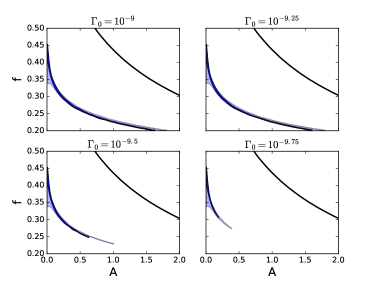
Figure 1: The $A-f$ diagram which coincides within 1$\sigma$ confidence level of Planck data. The corresponding values of $\Gamma_{0}$ are shown at the top of panels. The background transparent (foreground opaque) indicates $N=60$ ($N=50$). These values of $\Gamma_{0}$ are consistent with $R\gg 1$. The solid black curve shows the boundary $T=H$ and below the curve is consistent with $T>H$.

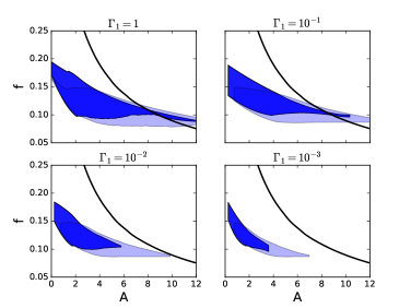
Figure 2: The $A-f$ region in the case of $\Gamma_{1}$ parametrization. These values of $\Gamma_{1}$ are consistent with $R\gg 1$. The solid black curve is same as Fig.(1).

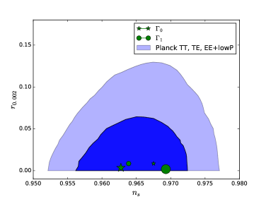
Figure 3: 1$\sigma$ and 2 $\sigma$ confidence regions borrowed from Planck Ade:2015lrj . Stars (squares) indicate warm inflation with $\Gamma_{0}$ ($\Gamma_{1}$) parametrization. Big and small points correspond to $N=60$ and $N=50$ respectively. For $\Gamma_{0}$ we set $f=0.28$, $A=0.35$ and $\Gamma_{0}=10^{-9}$. For $\Gamma_{1}$ we set $f=0.13$, $A=3.$ and $\Gamma_{1}=10^{-3}$.

At this point we would like to mention that in the high-dissipation regime $R\gg 1$, there is always a region in $A-f$ plane which is consistent with the warm inflation condition $T>H$. To clarify this issue we plot in Fig.(4) the diagram of $\log_{10}\frac{T}{H}$ in the $A-f$ plane. The solid line corresponds to the boundary limit $T=H$. Clearly, based on the condition $T>H$ we can reduce the parameter space and thus producing one of the strongest existing constraints (to our knowledge) on $A$ and $f$. Note that in order to produce the above diagram we have fixed the initial values of $T$ and $H$ to those at the beginning of inflation. After the triggering of inflation the inflaton/photon interaction takes place which leads to radiation production and thus it guarantees that the above condition holds during the inflationary era.

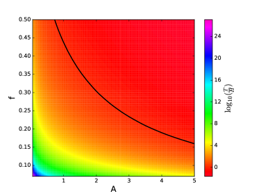
Figure 4: The value of $\frac{T}{H}$ at beginning of inflation in A-f plane. The solid black curve shows boundary $T=H$.

Finally, we investigate the possibility to treat $\lambda$ as a free parameter. In fact there are three main conditions which we need to use in order to provide a viable limit on the $\lambda$. These are: (a) the high dissipation regime $R\gg 1$, (b) the warm inflation condition $T>H$ and (c) to recover the Planck2015 $(n_{s},r)$ observational constraints. Our investigation shows that $\lambda$ is correlated with the $(A,f)$ pair. For example for $(A,f)=(0.5,0.25)$ we find $\lambda>6\times 10^{-16}$ which is consistent with above conditions while for $(A,f)=(0.4,0.2)$ we obtain $\lambda>1.5\times 10^{-20}$. In general we verify that it is not possible to find a lower value of $\lambda$ for all pairs of $(A,f)$.

5 Appendix

In this paper we have studied our model in natural unit ($\frac{h}{2\pi}=c=1$) therefore we have ($[\rm mass]=M$, $[\rm time]=T$ and $[\rm length]=L$ where $[A]$ means dimension of "$A$")

$$[c]=LT^{-1}=1~{}~{}~{}~{}~{}~{}~{}~{}~{}~{}~{}~{}~{}[h]=ML^{2}T^{-1}$$ (51)

$$\Rightarrow~{}~{}~{}~{}T=L=M^{-1}~{}~{}~{}~{}~{}~{}~{}~{}~{}~{}~{}~{}~{}~{}~{}~{}.$$

Using Eq.(5) we have

$$[H^{2}]=[\frac{8\pi}{M^{2}}\rho_{\phi}(1+\frac{\rho_{\phi}}{2\lambda})]~{}~{}~{}~{}~{}~{}~{}~{}~{}~{}~{}~{}~{}~{}~{}~{}~{}~{}~{}~{}~{}~{}~{}$$ (52)

$$\Rightarrow\frac{[a^{2}]}{[a^{2}]T^{2}}=\frac{[\rho_{\phi}]}{[M^{2}]}\Rightarrow~{}~{}~{}[\rho_{\phi}]=[T_{\mu}^{\nu}]=[P_{s}]=M^{4}$$

where $\rho_{\phi}$ is the scalar field energy density with dimension $M^{4}$. From Eq.(3) we have

$$[\dot{\phi}]=1~{}~{}~{}\Rightarrow~{}~{}~{}~{}[\phi]=M^{-1}$$ (53)

It appears that the tachyon scalar field has dimensions of $M^{-1}$. In Eq.(6) r.h.s and l.h.s have dimension $M^{4}$

$$[\dot{\rho_{\phi}}]+[3H\rho_{\phi}]+[3HP_{\phi}]=[\Gamma\dot{\phi}^{2}]$$ (54)

$$\Rightarrow~{}~{}\frac{[\rho_{\phi}]}{T}+\frac{[\rho_{\phi}]}{T}+\frac{[P_{\phi}]}{T}=[\Gamma]$$

$$~{}~{}\Rightarrow[\Gamma]=M^{5}~{}~{}~{}~{}~{}~{}~{}~{}~{}~{}~{}~{}~{}~{}~{}.$$

Now based on Eq.(12) we find

$$[R]=\frac{[\Gamma]}{[H][\rho_{\phi}]}=\frac{M^{5}}{MM^{4}}=1.$$ (55)

6 Conclusions

In this article we investigate the warm inflation for the Friedmann-Robertson-Walker spatially flat cosmological model in which the scale factor of the universe satisfies the form of Barrow Barrow:1996bd , namely $a(t)=a_{I}\exp(At^{f})$ ($0<f<1$). Within this context, we estimate analytically the slow-roll parameters and we compare our predictions with those of other inflationary models as well as we test the performance of warm inflation against the observational data. We find that currently warm inflationary model is consistent with the results given by Planck 2015 within $1\sigma$ uncertainties.

- (1) A.H. Guth, Phys. Rev. D23, 347 (1981). DOI 10.1103/PhysRevD.23.347
- (2) A. Albrecht, P.J. Steinhardt, Phys. Rev. Lett. 48, 1220 (1982). DOI 10.1103/PhysRevLett.48.1220
- (3) Y. Shtanov, J.H. Traschen, R.H. Brandenberger, Phys. Rev. D51, 5438 (1995). DOI 10.1103/PhysRevD.51.5438
- (4) L. Kofman, A.D. Linde, A.A. Starobinsky, Phys. Rev. D56, 3258 (1997). DOI 10.1103/PhysRevD.56.3258
- (5) A. Berera, Phys. Rev. Lett. 75, 3218 (1995). DOI 10.1103/PhysRevLett.75.3218
- (6) A. Berera, Phys. Rev. D55, 3346 (1997). DOI 10.1103/PhysRevD.55.3346
- (7) L.M.H. Hall, I.G. Moss, A. Berera, Phys. Rev. D69, 083525 (2004). DOI 10.1103/PhysRevD.69.083525
- (8) I.G. Moss, Phys. Lett. B154, 120 (1985). DOI 10.1016/0370-2693(85)90570-2
- (9) A. Berera, Nucl. Phys. B585, 666 (2000). DOI 10.1016/S0550-3213(00)00411-9
- (10) C. Armendariz-Picon, T. Damour, V.F. Mukhanov, Phys. Lett. B458, 209 (1999). DOI 10.1016/S0370-2693(99)00603-6
- (11) A. Sen, JHEP 04, 048 (2002). DOI 10.1088/1126-6708/2002/04/048
- (12) A. Sen, Mod. Phys. Lett. A17, 1797 (2002). DOI 10.1142/S0217732302008071
- (13) M. Sami, P. Chingangbam, T. Qureshi, Phys. Rev. D66, 043530 (2002). DOI 10.1103/PhysRevD.66.043530
- (14) G.W. Gibbons, Phys. Lett. B537, 1 (2002). DOI 10.1016/S0370-2693(02)01881-6
- (15) N. Arkani-Hamed, S. Dimopoulos, G.R. Dvali, Phys. Lett. B429, 263 (1998). DOI 10.1016/S0370-2693(98)00466-3
- (16) N. Arkani-Hamed, S. Dimopoulos, G.R. Dvali, Phys. Rev. D59, 086004 (1999). DOI 10.1103/PhysRevD.59.086004
- (17) I. Antoniadis, N. Arkani-Hamed, S. Dimopoulos, G.R. Dvali, Phys. Lett. B436, 257 (1998). DOI 10.1016/S0370-2693(98)00860-0
- (18) P. Binetruy, C. Deffayet, D. Langlois, Nucl. Phys. B565, 269 (2000). DOI 10.1016/S0550-3213(99)00696-3
- (19) P. Binetruy, C. Deffayet, U. Ellwanger, D. Langlois, Phys. Lett. B477, 285 (2000). DOI 10.1016/S0370-2693(00)00204-5
- (20) T. Shiromizu, K.i. Maeda, M. Sasaki, Phys. Rev. D62, 024012 (2000). DOI 10.1103/PhysRevD.62.024012
- (21) R. Maartens, D. Wands, B.A. Bassett, I. Heard, Phys. Rev. D62, 041301 (2000). DOI 10.1103/PhysRevD.62.041301
- (22) J.M. Cline, C. Grojean, G. Servant, Phys. Rev. Lett. 83, 4245 (1999). DOI 10.1103/PhysRevLett.83.4245
- (23) C. Csaki, M. Graesser, C.F. Kolda, J. Terning, Phys. Lett. B462, 34 (1999). DOI 10.1016/S0370-2693(99)00896-5
- (24) D. Ida, JHEP 09, 014 (2000). DOI 10.1088/1126-6708/2000/09/014
- (25) R.N. Mohapatra, A. Perez-Lorenzana, C.A. de Sousa Pires, Phys. Rev. D62, 105030 (2000). DOI 10.1103/PhysRevD.62.105030
- (26) R. Herrera, N. Videla, M. Olivares, Eur. Phys. J. C75(5), 205 (2015). DOI 10.1140/epjc/s10052-015-3433-6
- (27) J.D. Barrow, Class. Quant. Grav. 13, 2965 (1996). DOI 10.1088/0264-9381/13/11/012
- (28) L. Randall, R. Sundrum, Phys. Rev. Lett. 83, 4690 (1999). DOI 10.1103/PhysRevLett.83.4690
- (29) Y.F. Cai, J.B. Dent, D.A. Easson, Phys. Rev. D83, 101301 (2011). DOI 10.1103/PhysRevD.83.101301
- (30) R. Herrera, S. del Campo, C. Campuzano, JCAP 0610, 009 (2006). DOI 10.1088/1475-7516/2006/10/009
- (31) S. del Campo, R. Herrera, J. Saavedra, Eur. Phys. J. C59, 913 (2009). DOI 10.1140/epjc/s10052-008-0848-3
- (32) M.R. Setare, V. Kamali, JCAP 1208, 034 (2012). DOI 10.1088/1475-7516/2012/08/034
- (33) M.R. Setare, V. Kamali, JHEP 03, 066 (2013). DOI 10.1007/JHEP03(2013)066
- (34) X.M. Zhang, J.Y. Zhu, JCAP 1402, 005 (2014). DOI 10.1088/1475-7516/2014/02/005
- (35) L. Kofman, A.D. Linde, JHEP 07, 004 (2002). DOI 10.1088/1126-6708/2002/07/004
- (36) P. Brax, C. van de Bruck, Class. Quant. Grav. 20, R201 (2003). DOI 10.1088/0264-9381/20/9/202
- (37) T. Clifton, P.G. Ferreira, A. Padilla, C. Skordis, Phys. Rept. 513, 1 (2012). DOI 10.1016/j.physrep.2012.01.001
- (38) M. Bastero-Gil, A. Berera, R.O. Ramos, J.G. Rosa, JCAP 1301, 016 (2013). DOI 10.1088/1475-7516/2013/01/016
- (39) M. Bastero-Gil, A. Berera, R.O. Ramos, J.G. Rosa, JCAP 1410(10), 053 (2014). DOI 10.1088/1475-7516/2014/10/053
- (40) S. Bartrum, M. Bastero-Gil, A. Berera, R. Cerezo, R.O. Ramos, J.G. Rosa, Phys. Lett. B732, 116 (2014). DOI 10.1016/j.physletb.2014.03.029
- (41) M. Bastero-Gil, A. Berera, R. Cerezo, R.O. Ramos, G.S. Vicente, JCAP 1211, 042 (2012). DOI 10.1088/1475-7516/2012/11/042
- (42) M.R. Setare, V. Kamali, Phys. Rev. D87, 083524 (2013). DOI 10.1103/PhysRevD.87.083524
- (43) M.R. Setare, V. Kamali, Phys. Lett. B739, 68 (2014). DOI 10.1016/j.physletb.2014.10.006
- (44) M.R. Setare, V. Kamali, Phys. Lett. B736, 86 (2014). DOI 10.1016/j.physletb.2014.07.008
- (45) E.W. Kolb, M.S. Turner, The Early Universe (Addison-Wesley Publishing Company, 1990)
- (46) A.N. Taylor, A. Berera, Phys. Rev. D62, 083517 (2000). DOI 10.1103/PhysRevD.62.083517
- (47) R.O. Ramos, L.A. da Silva, JCAP 1303, 032 (2013). DOI 10.1088/1475-7516/2013/03/032
- (48) M. Bastero-Gil, A. Berera, I.G. Moss, R.O. Ramos, JCAP 1405, 004 (2014). DOI 10.1088/1475-7516/2014/05/004
- (49) D. Lyth, A. Liddle, The Primordial Density Perturbation (Cambridge U.P: Cambridge, 2009)
- (50) D. Langlois, R. Maartens, D. Wands, Phys. Lett. B489, 259 (2000). DOI 10.1016/S0370-2693(00)00957-6
- (51) M. Bastero-Gil, A. Berera, N. Mahajan, R. Rangarajan, Phys. Rev. D87(8), 087302 (2013). DOI 10.1103/PhysRevD.87.087302
- (52) A. Berera, M. Gleiser, R.O. Ramos, Phys. Rev. D58, 123508 (1998). DOI 10.1103/PhysRevD.58.123508
- (53) J. Yokoyama, A.D. Linde, Phys. Rev. D60, 083509 (1999). DOI 10.1103/PhysRevD.60.083509
- (54) A. Deshamukhya, S. Panda, Int. J. Mod. Phys. D18, 2093 (2009). DOI 10.1142/S0218271809016168
- (55) M.R. Setare, M.J.S. Houndjo, V. Kamali, Int. J. Mod. Phys. D22, 1350041 (2013). DOI 10.1142/S0218271813500417
- (56) M. Setare, V. Kamali, Phys. Rev. D91(12), 123517 (2015). DOI 10.1103/PhysRevD.91.123517
- (57) G. Panotopoulos, N. Videla, Eur. Phys. J. C75(11), 525 (2015). DOI 10.1140/epjc/s10052-015-3764-3
- (58) G. Arfken, in Mathematical Methods for Physicists (FL: Academic Press, Orlando, 1985)
- (59) I.A.S. M. Abramowitz, in Handbook of Mathematical Functions with Formu- las, Graphs, and Mathematical Tables, 9th printing (New York: Dover, 1972)
- (60) J.D. Barrow, A.R. Liddle, C. Pahud, Phys. Rev. D74, 127305 (2006). DOI 10.1103/PhysRevD.74.127305
- (61) J.D. Barrow, A.R. Liddle, Phys. Rev. D47, 5219 (1993). DOI 10.1103/PhysRevD.47.R5219
- (62) P.A.R. Ade, et al., (2015)
- (63) P. Ade, et al., Phys. Rev. Lett. 114, 101301 (2015). DOI 10.1103/PhysRevLett.114.101301
- (64) J. Martin, C. Ringeval, V. Vennin, Phys. Dark Univ. 5-6, 75 (2014). DOI 10.1016/j.dark.2014.01.003
- (65) M. Bastero-Gil, A. Berera, Phys. Rev. D76, 043515 (2007). DOI 10.1103/PhysRevD.76.043515
- (66) A.D. Linde, Phys. Lett. B129, 177 (1983). DOI 10.1016/0370-2693(83)90837-7
- (67) J.D. Barrow, Phys. Lett. B235, 40 (1990). DOI 10.1016/0370-2693(90)90093-L
- (68) J.D. Barrow, M. Lagos, J. Magueijo, Phys. Rev. D89(8), 083525 (2014). DOI 10.1103/PhysRevD.89.083525
- (69) A.A. Starobinsky, Phys. Lett. B91, 99 (1980). DOI 10.1016/0370-2693(80)90670-X
- (70) V.F. Mukhanov, G.V. Chibisov, JETP Lett. 33, 532 (1981). [Pisma Zh. Eksp. Teor. Fiz.33,549(1981)]
- (71) J. Ellis, D.V. Nanopoulos, K.A. Olive, JCAP 1310, 009 (2013). DOI 10.1088/1475-7516/2013/10/009
- (72) S. Basilakos, J.D. Barrow, Phys. Rev. D91, 103517 (2015). DOI 10.1103/PhysRevD.91.103517
- (73) C. Rubano, J.D. Barrow, Phys. Rev. D64, 127301 (2001). DOI 10.1103/PhysRevD.64.127301
- (74) G.R. Dvali, Q. Shafi, S. Solganik, in 4th European Meeting From the Planck Scale to the Electroweak Scale (Planck 2001) La Londe les Maures, Toulon, France, May 11-16, 2001 (2001). URL http://alice.cern.ch/format/showfull?sysnb=2256068
- (75) J. Garcia-Bellido, R. Rabadan, F. Zamora, JHEP 01, 036 (2002). DOI 10.1088/1126-6708/2002/01/036
- (76) A.S. Goncharov, A.D. Linde, Sov. Phys. JETP 59, 930 (1984). [Zh. Eksp. Teor. Fiz.86,1594(1984)]
- (77) G.R. Dvali, S.H.H. Tye, Phys. Lett. B450, 72 (1999). DOI 10.1016/S0370-2693(99)00132-X