Cascading DoS Attacks on IEEE 802.11 Networks

Abstract

We unveil the existence of a vulnerability in Wi-Fi (802.11) networks, which allows an adversary to remotely launch a Denial-of-Service (DoS) attack that propagates both in time and space. This vulnerability stems from a coupling effect induced by hidden nodes. Cascading DoS attacks can congest an entire network and do not require the adversary to violate any protocol. We demonstrate the feasibility of such attacks through experiments with real Wi-Fi cards, extensive ns-3 simulations, and theoretical analysis. The simulations show that the attack is effective both in networks operating under fixed and varying bit rates, as well as ad hoc and infrastructure modes. To gain insight into the root-causes of the attack, we model the network as a dynamical system and analyze its limiting behavior and stability. The model predicts that a phase transition (and hence a cascading attack) is possible when the retry limit parameter of Wi-Fi is greater or equal to 7, and characterizes the phase transition region in terms of the system parameters.

I Introduction

Wi-Fi (IEEE 802.11) is a technology widely used to access the Internet. Wi-Fi connectivity is provided by a variety of organizations operating over a shared RF spectrum. These include schools, libraries, companies, towns and governments, as well as ISP hotspots and residential wireless routers. Wi-Fi traffic is also rapidly rising due to increased offloading by cellular operators [1]. The importance of Wi-Fi networks and the need to strengthen their resilience to intentional and non-intentional interference have been recognized by companies, such as Cisco [2].

Wi-Fi networks rely on simple, distributed mechanisms to arbitrate access to the shared spectrum and optimize performance. Such mechanisms include carrier sensing multiple access (CSMA), exponential back-offs, and bit rate adaptation. The behavior of these mechanisms in isolated single-hop networks has been extensively studied and is generally well-understood (see, e.g., [3]). However, due to interference coupling, these mechanisms result in complex interactions in multi-hop settings. As a consequence, different networks do not always evolve independently, even if they are located far away.

Figure 1 serves to illustrate this phenomenon at a high level. Suppose that an attacker increases the rate at which it generates packets, and transmits these packets in accordance with the IEEE 802.11 protocol. These transmissions may cause packet collisions at nodes concurrently receiving packets from other sources. Due to the infamous hidden node problem, which is hard to avoid in wireless networks, transmitters may be unable to hear transmission by other nodes, even when using CSMA, and hence keep retransmitting packets until they reach the so-called retry limit of the back-off procedure. These retransmissions affect other neighbours and may propagate.

While an optional mechanism, called RTS/CTS, has been designed to combat the hidden node problem, it increases overhead and latency especially at high bit rates. Since the cost of the RTS/CTS exchange usually does not justify its benefits, it is commonly disabled [4, 5]. Indeed, most manufacturers of Wi-Fi cards disable RTS/CTS by default and discourage changing this setting as explicitly stated in [6, 7, 8, 9]. Therefore, most Wi-Fi systems today operate without RTS/CTS.

The coupling phenomenon induced by interferences creates multi-hop dependencies, which an adversary can take advantage of to launch a widespread network attack from a single location. We refer to such an attack as a cascading Denial-of-Service (DoS) attack. Cascading DoS attacks are especially dangerous because they affect the entire network and do not require the adversary to violate any protocol (i.e., the attacks are protocol-compliant).

The contributions of this paper are as follows. First, we unveil the existence of a vulnerability in the IEEE 802.11 standard, which allows an attacker to launch protocol-compliant cascading DoS attacks. In contrast to existing jamming attacks, the attacker does not need to be in the vicinity of the victims.

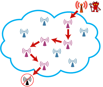
Figure 1: Illustration of a cascading denial of service attack. Transmissions by an attacker impact nodes located far away, due to interference coupling caused by hidden nodes.

Second, we provide a concrete attack that exploits this vulnerability in certain network scenarios. We demonstrate the attack through experiments on a testbed composed of nodes equipped with real Wi-Fi cards, and through extensive ns-3 simulations.

Third, we show the existence of a phase transition. When the packet generation rate of the attacker is lower than the phase transition point, it has vanishing effect on the rest of the network. However, once the packet generation rate exceeds the phase transition point, the network becomes entirely congested. Thus, under a phase transition, the utilization of a remote node experiences no change until it is suddenly forced to congestion [10].

Finally, we introduce a new analytical model that sheds light into the phase transition observed in the simulations and experiments. We apply fixed point theorems to this model. The analysis predicts for which values of the retry limit a phase transition (and hence a cascading attack) can occur, and explicitly characterizes the phase transition region in terms of the system parameters. In particular, we show that a phase transition can occur for the default value of the retry limit in Wi-Fi, which is 7. We carry out a stability analysis and demonstrate that in the phase transition region the system must have multiple fixed points, one of which being unstable.

The rest of the paper is organized as follows. In Section II, we discuss related work. In Section III, we provide brief background on Wi-Fi, hidden nodes, and Minstrel, and introduce our network model. We present and discuss experimental and simulation results in Section IV. In Section V, we present an analytical model that explains the behaviour of the network and the impact of various parameters, and compare the analytical and simulation results. In Section VI, we conclude the paper and discuss possible mitigation methods.

An earlier and shorter version of this paper appeared in the proceedings of the IEEE Conference on Communications and Network Security (CNS 2016) [11]. This journal version significantly expands the theoretical analysis, including detailed proofs of all the lemmas and theorems, and new results on stability analysis and heterogeneous traffic load, all of which can be found in Section V. Moreover, new simulation results for infrastructure networks, networks supporting RTS/CTS, ring networks, networks based on a realistic indoor building model, and networks with heterogeneous traffic load are presented in Sections IV-B and V-H.

II Related Work

In general, the main goal of a DoS attack is to make communication impossible for legitimate users. Within the context of wireless networks, a simple and popular means to launch a DoS attack is to jam the network with high power transmissions of random bits, hence creating interferences and congestion. Jamming at the physical layer, together with anti-jamming countermeasures, have been extensively studied (cf. [12] for a monograph on this subject).

More recently, several works have developed and demonstrated smart jamming attacks. These attacks exploit protocol vulnerabilities across various layers in the stack to achieve high jamming gain and energy efficiency, and a low probability of detection [13]. For instance, [14] shows that the energy consumption of a smart jamming attack can be four orders of magnitude lower than continuous jamming. The works in [15, 16] show that several Wi-Fi bit rate adaptation algorithms, such as SampleRate, ONOE, AMRR, and RARF, are vulnerable to smart jamming. However, both conventional and smart jamming attacks are usually non-protocol compliant. Moreover, they require physical proximity. These limitations can be used to identify and locate the jammer.

In contrast, in this work we show how a protocol-compliant DoS attack can be remotely launched by exploiting coupling due to hidden nodes in Wi-Fi. Rate adaptation algorithms further amplify this attack due to their inability to distinguish between collisions, interferences, and poor channels. One potential mitigation is to design a rate adaptation algorithm whose behaviour is based on the observed interference patterns [17, 18]. However, to the best of our knowledge, none of these rate adaptation algorithms are used in practice. Our work is based on Minstrel [19], which is the most recent, popular, and robust rate adaptation algorithm for Linux systems.

The attacks that we are investigating bear similarity to cascading failures in power transmission systems [20, 21]. When one of the nodes in the system fails, it shifts its load to adjacent nodes. These nodes in turn can be overloaded and shift their load further. This phenomenon has also been studied in wireless networks. For instance, [22, 23] model wireless networks as a random geometric graph topology generated by a Poisson point process. They use percolation theory to show that the redistribution of load induces a phase transition in the network connectivity. However, the cascading phenomenon that we investigate in this paper is different from cascading failure studied in those works. In our work, the exogenous generation of traffic at each node is independent. That is, a node will not shift its load to other nodes. The amount of traffic measured on the channel increases due to packet retransmissions caused by packet collisions, rather than due to traffic redistribution.

The work in [24, 25] show that interference coupling can affect the stability of multi-hop networks. In the case of a greedy source, a three-hop network is stable while a four-hop network becomes unstable. In contrast, in our work, the path of each packet consists of a single-hop. Thus, network instability is not due to multi-hop communication in our case.

The work in [26, 10] show that local coupling due to interferences can have global effects on wireless networks. Thus, [26] proposes a queuing-theoretic analysis and approximation to predict the probability of a packet collision in a multi-hop network with hidden nodes. It shows that the sequence of the packet collision probabilities in a linear network converges to a fixed point. The work in [10] evaluates the impact of rate adaption and finds out that traffic increase at a single node can congest an entire network, and points out the existence of a phase transition.

Our paper differs in several aspects. First, it considers an adversarial context, and shows how interference-induced coupling can be exploited to cause denial of service. Second, to our knowledge, it is the first work to demonstrate the existence of such coupling on real commodity hardware. Third, our simulations are based on a high-fidelity wireless simulator (ns-3), capable of capturing the effects of rate adaptation algorithms and accurately modeling infrastructure networks. Finally, our analytical model is original and captures the impact of the retry limit and traffic parameters. A key result is that a cascading attack can be launched for the default value of the retry limit in Wi-Fi, a result validated by the experiments and simulations.

III Background and Model

We first review key aspects of IEEE 802.11 and then describe the network model under consideration.

III-A Wi-Fi Summary

Wi-Fi is a wireless local area network (WLAN) technology, which mainly runs on 2.4 GHz ISM bands and 5 GHz bands [5]. The IEEE 802.11 standard is a series of specifications, such as the media access control (MAC) and physical layer (PHY) interfaces. The first 802.11 standard that gained widespread success is 802.11b. It runs on 2.4 GHz bands and has up to 11 Mb/s bit rate. The subsequent standards (e.g., 802.11a, g, n, and ac) increased the bit rates using higher order modulation along with coding, OFDM, MIMO, and wider bands. It is noteworthy that 802.11b is the only mode that supports communication at 1 Mb/s. Hence, when the bit rate reduces to 1 Mb/s, Wi-Fi network reverts to the 802.11b mode. Generally, this lower bit rate has higher resistance to interference during transmission and is able to operate over lower SNR channels.

The IEEE 802.11 standard uses a CSMA/CA mechanism to control access to the transmission medium and avoid collisions. After a packet is sent, a node waits for a short interframe slots (SIFS) period to receive an ACK. Whenever the channel becomes idle, the node waits for a distributed interframe space (DIFS $>$ SIFS) period and a random backoff before contending for the channel. The random backoff consists of a random number of backoff slots, which depends on the so-called contention window. Specifically, at the $r\geq 1$ retransmission attempt (retry count), the contention window $CW_{r}$ is given by

$$CW_{r}=\left\{\begin{array}[]{ll}2^{r-1}(CW_{1}+1)-1&CW_{r}<CW_{max},\\ CW_{max}&\text{otherwise}.\end{array}\right.$$ (3)

The number of backoff slots is chosen uniformly at random in the interval $[0,CW_{r}]$. For IEEE 802.11b, the initial contention window size is $CW_{1}=31$ , the maximum contention window size is $CW_{max}=1023$, and the duration of a backoff slot is $20~{}\mu s$. Note that the case $r=1$ corresponds to the initial packet transmission attempt.

III-B Hidden Node Problem

A typical instance of the hidden node problem is illustrated in Figure 2. The figure shows three nodes: a transmitter, a receiver and a hidden node. The dashed circle represents the transmission range of the node. Since the transmitter and the hidden node cannot sense each other, a collision happens when both of them transmit packets at the same time.

A packet collision triggers a retransmission. In IEEE 802.11, there is an upper limit on the number of retransmissions that a packet can incur, called retry limit and denoted by $R$ (the default value is $R=7$). If the retry count $r$ of a packet exceeds the retry limit, the packet is dropped, the retry count is reset to $r=1$, and a new packet transmission can start. The channel utilization of a node increases with the probability of a packet collision. In the worst case, the utilization can be $R$ times larger than in the absence of packet collisions. Therefore, the access channel of a node can easily be saturated if it is forced to retransmit packets.

The hidden node problem can in principle be avoided by enabling the RTS/CTS exchange, which is implemented in Wi-Fi networks. However, the RTS/CTS exchange has not only high overhead, but also does not always fully prevent packet collisions [27] and may lead to deadlocks in multi-hop configurations [28]. Generally, it is either turned off [29] or only used for packets whose length exceeds the so-called RTS threshold. Most manufacturers of Wi-Fi cards, including Netgear [6], TP-LINK [7], Linksys [8] and D-Link [9], disable RTS/CTS altogether by setting the RTS threshold to a sufficiently high default value (e.g., 2346 bytes, which corresponds to the maximum length of an IEEE 802.11 frame). They furthermore recommend to not change the default setting.

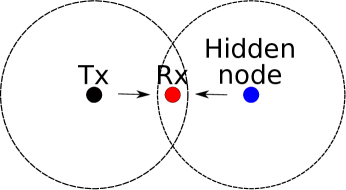
Figure 2: Classical hidden node problem. The transmitter and the hidden node cannot sense each other. The collision happens when they transmit simultaneously.

III-C Minstrel Rate Adaptation

Minstrel is a practical, state-of-the-art rate adaptation algorithm that has been implemented within the MadWiFi project and Linux mac80211 driver framework [19]. It chooses the bit rate of a transmission based on the throughput measured over past transmissions at different rates. Technically, it selects a bit rate following a retry chain, as shown in Table I.

In Minstrel, 90% of the packets are transmitted at a “normal rate” (fourth column in Table I). The remaining 10% are transmitted at a “lookaround rate” (second and third columns in Table I). Each packet is transmitted at a rate following a retry chain (rows in Table I). For example, consider a packet being transmitted at “lookaround rate”. If a random rate is lower than the rate with “best throughput”, the packet is first transmitted at the “best throughput” rate, then at the “random rate”, then at the “best probability” rate, and finally at the “lowest baserate”. The packet is dropped if the transmission fails at the “lowest baserate”. The retry chain table is updated 10 times every second based on performance statistics.

Therefore, a large amount of packet loss does not necessarily cause Minstrel to switch to a low bit rate. Another advantage of Minstrel is that it probes the throughput of different bit rates randomly. This makes the rate adaptation more robust in complicated environment and against some adversaries.

TABLE I: Minstrel Retry Chain [19]

Try	Lookaround rate		Normal rate
	random $<$ best	random $>$ best
1	Best throughput	Random rate	Best throughput
2	Random rate	Best throughput	2nd best throughput
3	Best probability	Best probability	Best probability
4	Lowest baserate	Lowest baserate	Lowest baserate

III-D Network Model

The network model considered in this paper is shown in Figure 3. This configuration could arise over different time and space in more complex network topologies. We consider $N+1$ pairs of nodes. Each node $A_{i}$ ($i=0,1,2,\ldots$, $N$) transmits packets to node $B_{i}$. The dashed circle represents the range of transmission. Node $B_{i+1}$ can receive packets from both node $A_{i}$ and node $A_{i+1}$. However, node $A_{i}$ and node $A_{i+1}$ cannot hear each other. That is, node $A_{i}$ is a hidden node with respect to node $A_{i+1}$ (and vice-versa). A packet collision happens at node $B_{i+1}$ when packet transmissions by node $A_{i}$ and $A_{i+1}$ overlap.

We assume that all the nodes communicate over the same channel. Note that there are only three non-overlapping channels in the 2.4GHz band. Hence, it is common that several nodes use the same channel over time and space in crowded areas.

III-E Cascading DoS attack

Our goal is to investigate how node $A_{0}$ can trigger a cascading DoS attack, resulting in a congestion collapse over the entire network. We start by increasing the packet generation rate at node $A_{0}$. Node $A_{0}$ transmits packets over its channel, in compliance with the IEEE 802.11 standard. The transmissions by node $A_{0}$ cause packet collisions at node $B_{1}$. These collisions require node $A_{1}$ to retransmit packets. The increased amount of packet transmissions and retransmissions by node $A_{1}$ impact node $A_{2}$ and so forth. If this effect keeps propagating and amplifying, then the result is a network-wide denial of service, which we refer to as a cascading Denial of Service (DoS) attack. Because this attack is protocol-compliant, it is difficult to detect or trace back to the initiator.

We note here that as a hidden node retransmits its packets, it must back off after each retransmission, which leaves the channel idle for a certain period of time. However, the duration of the backoff period is generally too short to allow for a successful transmission. Indeed, a packet transmission is successful only if

1. The size of the contention window of the hidden node is longer than the packet transmission time.

2. The transmitter starts and ends its transmission entirely during the backoff period of the hidden node.

At 1 Mb/s, the transmission time of an 1500 bytes packet lasts 12 ms. This is longer than the contention window as long as $CW_{r}<CW_{max}=1023$. Hence, by Eq. (3), a transmission cannot be successful during the backoff period preceding the $r<6$ retransmission attempt by a hidden node.

At the $r\geq 6$ retransmission attempt by a hidden node $A_{i}$, $CW_{r}=CW_{max}=1023$. Node $A_{i}$ back-offs for $n$ slots, where $n$ is an integer between 0 and 1023 that is picked uniformly at random (i.e., with probability $1/1024$). Since the length of a backoff slot is 20 $\mu$s, the backoff delay is $0.02n$ ms. Without loss of generality, assume that node $A_{i}$ starts backing off at time $t=0$ and ends its backoff at time $t=0.02n$ (all the time units are in milliseconds). Node $A_{i}$ then starts a packet transmission, which ends at time $t=0.02n+0.12$.

Node $A_{i+1}$ can transmit a packet successfully only if it starts its transmission during the time interval $[0,0.02n-12]$. This requires $n>600$. Assuming that the starting time of the packet transmission by node $A_{i+1}$ is uniformly distributed in the time interval $[0,0.02n+12]$, the probability that a packet is successfully transmitted by node $A_{i+1}$ is

$$\sum_{n=600}^{1023}\frac{1}{1024}\cdot\frac{0.02n-12}{0.02n+12}=0.059.$$

Thus, the likelihood of a successful packet transmission is low, a result validated by the experimental and simulation results of the next section.

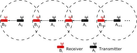
Figure 3: Topology of the network. Node $A_{i}$ transmits packets to node $B_{i}$. Node $A_{i}$ is a hidden node with respect to $A_{i+1}$.

IV Experimental and Simulation Results

In this section, we demonstrate the feasibility of launching cascading DoS attacks both through experiments and simulations. We first show results on an experimental testbed using real Wi-Fi cards. We then use ns-3.22 simulations to investigate how this attack can be performed in significantly larger scale networks, and under different settings (ad hoc, infrastructure, fixed bit rate, and adaptive bit rate).

IV-A Experiments

We set up an experimental testbed composed of six nodes. The testbed configuration is shown in Figure 4. We establish an IEEE 802.11n ad hoc network consisting of three pairs of nodes. Each node consists of a PC and a TP-LINK TL-WN722N Wireless USB Adapter. We use RF cables and splitters to link the nodes, isolate them from external traffic, and obtain reproducible results.

We place 70 dB attenuators on links between node $A_{i}$ and $B_{i}$ ($i\in 0,1,2$), and 60 dB attenuators on links between nodes $A_{i}$ and $B_{i+1}$. The difference in the signal attenuation of different links ensures that a packet loss occurs if a hidden node transmits. In practice, such a situation may occur if nodes $A_{i}$ and $B_{i+1}$ communicate without obstacles, while node $A_{i}$ and $B_{i}$ are separated by an office wall [30]. The transmission power of each node is set to 0 dBm. We use iPerf [31] to generate UDP data streams and to measure the throughput achieved on each node. The length of a packet is the default IP packet size of 1500 bytes.

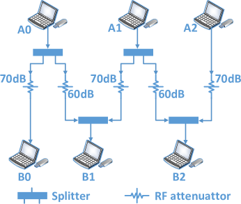
Figure 4: Experimental testbed.

Figure 5 demonstrates the cascading DoS attack on the experimental testbed. At first, the packet generation rates of nodes $A_{0},A_{1}$ and $A_{2}$ are set to 400 Kb/s. We observe that the throughput of all the nodes remains in the vicinity of 400 Kb/s during the first 300 seconds. After 300 seconds, $A_{0}$ starts transmitting packets at 1 Mb/s. As a result, the throughput of nodes $A_{1}$ and $A_{2}$ suddenly vanishes. Once node $A_{0}$ resumes transmitting at 400 Kb/s, the throughput of node $A_{1}$ and node $A_{2}$ recovers.

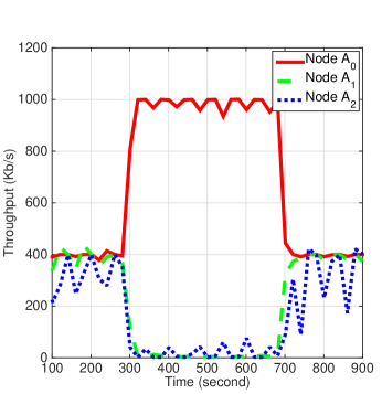
Figure 5: Throughput performance measurements in testbed. When node $A_{0}$ starts increasing its packet generation rate, the throughput of nodes $A_{1}$ and $A_{2}$ vanishes.

IV-B Simulations

In the previous section, we demonstrated the feasibility of launching a cascading DoS attack on an experimental testbed. This testbed relies on commercial cards that are black boxes for all purposes. For instance, the driver of the Wi-Fi card and the rate adaptation algorithm are closed-source. There are also substantial usage restrictions, such as parameter settings.

In order to gain a better insight into the attack in large-scale networks, we resort to ns-3 simulations, a state-of-the-art simulator which includes high-fidelity wireless libraries. We show the occurrence of cascading DoS attacks

1. In ad hoc networks with fixed bit rate;

2. In ad hoc networks under Minstrel rate adaptation;

3. In infrastructure networks;

4. In ring topology networks;

5. In an indoor scenario;

and the countering of cascading DoS attacks

1. In networks with RTS/CTS enabled.

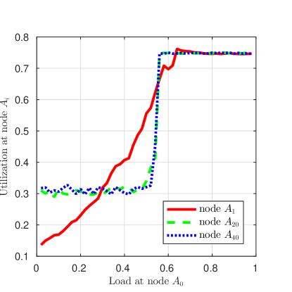
(a) As the traffic load at node $A_{0}$ increases, the utilization of remote nodes (e.g., $A_{20}$ and $A_{40}$) exhibits a phase transition.

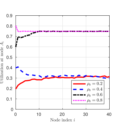
(b) Utilization of nodes $A_{i}$ ($i\geq 1$) for different traffic loads at node $A_{0}$. The utilization converges as $i$ gets large. When the load at node $A_{0}$ changes from $0.4$ to $0.6$, the sequence of utilization converge to different limits, illustrating the phase transition.

Figure 6: Occurrence of cascading DoS attacks in ad hoc networks with fixed bit rate.

IV-B1 Fixed bit rate

We first describe the occurrence of a cascading DoS attack in an ad hoc network with fixed bit rate. We consider a linear topology consisting of 41 pairs of nodes (i.e. a sequence of 41 hidden nodes), as shown in Figure 3. Each packet is transmitted over a single-hop path (similar to Wi-Fi Direct). We fix the bit rate to 1 Mb/s and the retry limit to $R=7$.

We set up a Wi-Fi network using the standard IEEE 802.11 library in ns-3. At each node $A_{i}$, $i\geq 1$, the generation rate of UDP packets is $\lambda_{i}=8.125$ pkts/s. The generation rate of UDP packets at node $A_{0}$, $\lambda_{0}$, varies from $1.25$ to $61.25$ pkts/s. Packets at each node are generated according to a Poisson process, hence different nodes start transmitting at different times. The size of each packet is 2000 bytes. Each node has the same transmission power (40 mW). We set the propagation loss between node $A_{i}$ and $B_{i}$ to 80 dB and the propagation loss between node $A_{i}$ and $B_{i+1}$ to 70 dB. We run each simulation five times for 1,000 seconds, and average out the results.

The (exogenous) load at each node $A_{i}$ is denoted $\rho_{i}=\lambda_{i}T$, where $T$ represents the duration of each packet transmission attempt (0.016 second in our case). The utilization of a node $A_{i}$, denoted $u_{i}$, is defined as the fraction of time the node is busy transmitting bits on the channel.

Figure 6(a) depicts the utilization $u_{1}$, $u_{20}$, and $u_{40}$ as a function of $\rho_{0}$, the load at node $A_{0}$. The utilization of node $A_{1}$, $u_{1}$, increases smoothly until it reaches its upper limit. However, the utilizations of nodes $A_{20}$ and $A_{40}$ remain low until $u_{0}$ reaches a certain threshold around $\rho_{0}=0.5$, at which point $u_{20}$ and $u_{40}$ suddenly jump to a high value. This sudden jump corresponds to a phase transition, and the critical threshold represents the phase transition point.

Figure 6(b) illustrates the phase transition in a different way. The figure depicts the utilization of each node $A_{i}$ for $i\geq 1$, as $i$ increases. Again, we observe that different values of $\rho_{0}$ lead to two completely distinct behaviour for the sequence of utilizations $(u_{i})_{i=0}^{40}$ (i.e., $u_{40}\simeq 0.3$ when $\rho_{0}=0.2$ and $\rho_{0}=0.4$, while $u_{40}\simeq 0.75$ when $\rho_{0}=0.6$ and $\rho_{0}=0.8$). Note that the upper limit of the utilization does not reach 1, due to inter-frame spacing requirements and (random) backoff delays mandated by IEEE 802.11.

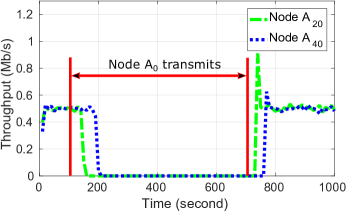
(a) Throughput

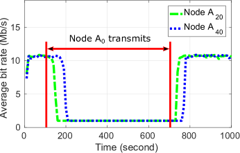
(b) Bit rate

Figure 7: Simulation results with Minstrel rate adaptation. When node $A_{0}$ generates packets at 5 Mb/s and transmits, the throughput of nodes $A_{20}$ and $A_{40}$ vanishes. The average bit rates of nodes $A_{20}$ and $A_{40}$ also reduce to 1 Mb/s. This result indicates that nodes $A_{20}$ and $A_{40}$ are transmitting packets at the lowest bit rate, however with no throughput (all their packets collide).

IV-B2 Rate Adaptation

We next consider the same network setting as in the previous section, but this time we assume that nodes can transmit at different bit rates. We specifically assume that nodes implement the Minstrel rate adaptation algorithm. In this case, the attack works by coercing the rate adaptation algorithm to reduce the bit rate to 1 Mb/s at each node, thus leading to similar results to those shown in Section IV-B1. In our simulations, the parameter EWMA of Minstrel is set to 0.25 [32].

We set $\lambda_{0}=312.5$ pkts/s and $\lambda_{i}=31.25$ pkts/s ($i\geq 1$) for the packet generation rates. As shown in Figure 7, packet transmissions at node $A_{0}$ start after $t=100$ s. During the first 100 seconds, the throughput of nodes $A_{20}$ and $A_{40}$ remain around 0.5 Mb/s, which implies that all the packets are received. Once node $A_{0}$ starts transmitting packets, the throughput of nodes $A_{20}$ and $A_{40}$ is brought down to close to zero. We also observe that the bit rates at node $A_{20}$ and $A_{40}$ go down to 1 Mb/s, due to the repeated packet collisions. Once node $A_{0}$ stops transmitting at $t=700$ s, nodes $A_{20}$ and $A_{40}$ recover.

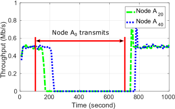
(a) When node $A_{0}$ generates packets at 5 Mb/s and transmits, the throughput of nodes $A_{20}$ and $A_{40}$ vanishes.

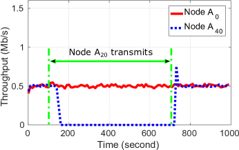
(b) When node $A_{20}$ generates packets at 5 Mb/s and transmits, the throughput of node $A_{40}$ vanishes while the throughput of node $A_{0}$ does not.

Figure 8: Simulation results under AP mode without reassociation. Nodes $A_{i}$ are stations and nodes $B_{i}$ are access points, for $i\in\{0,1,2,\dots\}$.

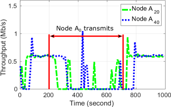
Figure 9: Simulation results under AP mode with reassociation. When node $A_{0}$ generates packets at 5 Mb/s and transmits, the throughput of node $A_{20}$ and $A_{40}$ significantly decreases.

IV-B3 Infrastructure networks

We next show that cascading DoS attacks are also feasible in infrastructure networks. Since the infrastructure mode is more widely used than ad hoc in practice, the feasibility of the cascading DoS attack in infrastructure networks increases its severity and potential impact. We repeat the simulations of Section IV-B2 except that we set nodes $B_{i}$ as access points, and nodes $A_{i}$ as stations. The initial beacon starting time at each AP is a random variable that is uniformly distributed between 0 and $102.4$ ms.

We first investigate the cases where stations do not restart association when beacons are missing. Toward this end, we set the number of consecutive beacons that must be missed before restarting association, i.e. the attribute MaxMissBeacons in ns-3, to a large value. Otherwise, we use the default settings of ns-3 for the APs [33] and the stations [34]. Figure 8 shows similar results as in Section IV-B2, namely when a cascading DoS attack is launched by node $A_{0}$, as shown in Figure 8(a), the remote nodes $A_{20}$ and $A_{40}$ in the sequence exhibit a phase transition. If the attacker is node $A_{20}$, the simulation result in Figure 8(b) shows that the throughput of node $A_{40}$ vanishes but the throughput of node $A_{0}$ does not. This result shows that an attack can be launched from any node $A_{i}$ in the topology and the following nodes in the sequence (i.e., $A_{i+1},A_{i+2},\ldots$) will experience congestion.

We next consider the case where stations restart association when beacons are missing. We set ${\tt MaxMissBeacons}=10$, which is the default value in ns-3 [34]. The simulation results are shown in Figure 9. When Node $A_{0}$ starts to transmit packets, we observe a significant throughput degradation at nodes $A_{20}$ and $A_{40}$, but the throughput does not vanish completely. The reason is that if $A_{i}$ disassociates from its AP $B_{i}$ over a certain period then node $A_{i+1}$ is not affected by interference coupling during that period. This result indicates that reassociations help mitigate cascading DoS attacks, though throughput performance is still significantly impaired.

IV-B4 Ring topology

We investigate cascading DoS attacks in a ring topology with 41 pairs of nodes, as shown in Figure 10. In our previous results for linear topologies, the effect of an attack disappears once the attacker reduces its packet generation rate. However, the effect of an attack in a ring topology can last for a long period of time after the attack stops. Node $A_{i}$ $(i=0,1,\dots)$ generate packets at rate 0.5 Mb/s, following a Poisson process. At time $t=300$ s, node $A_{0}$ increases its packet generation rate to 11 Mb/s and the throughput of all the nodes vanishes. Yet, unlike results in linear topologies, the throughput of the nodes does not recover after node $A_{0}$ reduces its packet generation rate back to 0.5 Mb/s. The cyclic nature of the topology reinforces the attack even after the trigger stops.

This result is illustrated in Figure 11. During the first 100 seconds, all the nodes $A_{i}$ $(i=0,1,\dots)$ generate packets at 0.5 Mb/s. At time $t=300$ s, node $A_{0}$ increases its packet generation rate to 11 Mb/s. As a result, the throughput of all nodes vanishes. Yet, unlike results in linear topologies, the throughput of the nodes does not recover after node $A_{0}$ reduces its packet generation rate back to 0.5 Mb/s. The cyclic nature of the topology reinforces the attack even after the trigger stops.

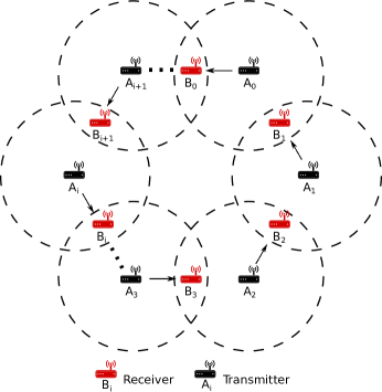
Figure 10: Ring topology under cascading DoS attack. The dash circle represents the transmission range of the transmitter.

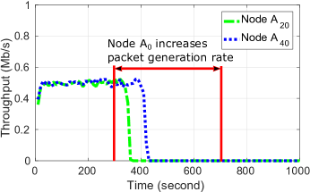
Figure 11: Simulation results under a ring topology. When the packet generation rate of node $A_{0}$ increases, the throughput of nodes $A_{20}$ and $A_{40}$ vanishes. This effect continues even when the packet generation rate of node $A_{0}$ decreases.

IV-B5 Building model

In this section, we use the ns-3 HybridBuildingsPropagationLossModel library [35] to demonstrate the feasibility of cascading DoS attacks in an indoor scenario. Models in this library realistically characterize the propagation loss across different spectrum bands (i.e., ranging from 200 MHz to 2.6 GHz), different environments (i.e., urban, suburban, open areas), and different node positions with respect to buildings (i.e., indoor, outdoor and hybrid). The building models take into account the penetration losses of the walls and floors, based on the type of buildings (i.e., residential, office, and commercial).

In our simulations, we consider a 20-floor office building with six rooms in each floor, as shown in Figure 12. We assume that five pairs of Wi-Fi nodes $(A_{i},B_{i})$ are active in the building, where node $A_{i}$ transmits packets to nodes $B_{i}$ ($i=0,1,2,3,4$). The bit rate is set to 1 Mb/s, the retry limit to $R=7$, and the frequency to 2.4 GHz. The generation rate of UDP packets at nodes $A_{i}$, $i\geq 1$, is $\lambda_{i}=8.125$ pkts/s. Packets are 2000 bytes long.

We turn on and off transmissions at node $A_{0}$ to observe how it impacts the throughput of other nodes. Simulation results are shown in Figure 13. When node $A_{0}$ does not transmit, the throughput of node $A_{4}$ is 0.13 Mb/s and it incurs no packet loss. However, when node $A_{0}$ starts transmitting, the throughput of node $A_{4}$ collapses. The throughput of node $A_{4}$ recovers only after node $A_{0}$ stops transmitting.

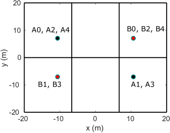
(a) Top view.

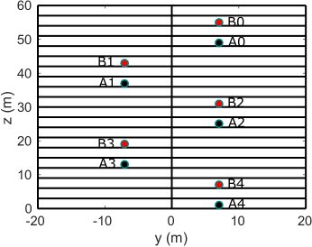
(b) Side view.

Figure 12: Office building model. The building has 20 floors ($z$-axis) and 6 rooms in each floor ($x$ and $y$ axes).

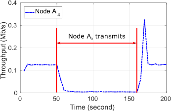
Figure 13: Simulation results using ns-3 building model. When node $A_{0}$ transmits, the throughput of remote node $A_{4}$ collapses.

IV-B6 RTS/CTS

We next evaluate the impact of enabling RTS/CTS in the topology under consideration. Specifically, we repeat the simulations of Section IV-B2, but with RTS/CTS enabled. Figure 14 shows that transmissions by node $A_{0}$, which start after $100$ s, have no effect on the throughput of remote nodes $A_{20}$ and $A_{40}$. This shows that RTS/CTS is an effective solution against cascading DoS attacks in this scenario.

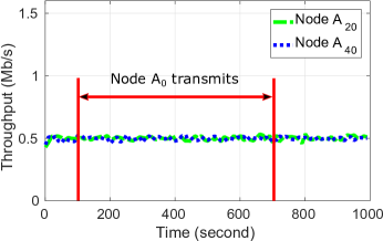
Figure 14: Simulation results when enable RTS/CTS. The increase of the packet generation rate of node $A_{0}$ does not affect the throughput of nodes $A_{20}$ and $A_{40}$.

V Analysis

In this section, we develop a stylized, analytical model that provides qualitative insight into the network behavior observed in the simulations and experiments for the linear topology. Specifically, our goal is to explain why and under what conditions the phase transition occurs, and shed light into the roles played by the retry limit $R$ and the traffic load at the different nodes.

V-A Model

We consider the linear topology shown in Figure 3. Packet generations at each node $A_{i}$ form a Poisson process with rate $\lambda_{i}$. The packet size is fixed and the duration of each packet transmission attempt is $T$ (we assume a fixed bit rate). A transmission by node $A_{i+1}$ is successful only if does not overlap with any transmission by (hidden) node $A_{i}$.

If a packet collides, it is retransmitted until either it is successfully received or the retry count reaches the limit $R$. Let $1\leq\overline{r}_{i}\leq R$ represent the mean retry count at node $A_{i}$. Note that the initial packet transmission is included in that count. Then, the mean service time of a packet at node $A_{i}$ is $\overline{r}_{i}T$. To keep the analysis tractable, timing details of Wi-Fi, such as DIFS, SIFS, and back-off inter-frame spacing are ignored. Therefore the upper limit of the utilization equals 1 in our analysis.

We denote the utilization of node $A_{i}$ by $0\leq u_{i}\leq 1$, where $u_{i}$ represents the fraction of time node $A_{i}$ transmits. If $u_{i}=1$, node $A_{i}$ is congested and transmits continuously. Otherwise, node $A_{i}$ is uncongested and transmits packets at rate $\overline{r}_{i}\lambda$. Therefore, the utilization of node $A_{i}$ for all $i\geq 0$ is

$$u_{i}=\min\{\overline{r}_{i}\lambda_{i}T,1\}.$$ (4)

Note that there is no retransmission at node $A_{0}$ and $\overline{r}_{0}=1$.

Our model represents a special case of interacting queues, which are notoriously difficult to analyze [36]. To make the analysis tractable, we assume that:

1. Packet transmissions and retransmissions at each uncongested node $A_{i}$ form a Poisson process with rate $\overline{r}_{i}\lambda$.

2. The probability that a packet transmitted by node $A_{i}$ collides is independent of previous attempts. This probability is denoted $p_{i}$.

Though the assumption of Poisson retransmissions is not fully consistent with the Wi-Fi protocol, it is similar to the “random-look” model used by Kleinrock and Tobagi in their analysis of (single hop) random access networks [37] (see also [38][Ch. 4]). The simulations do not incorporate the simplifications used to make the analysis tractable, yet lead to the same effects. We stress that beside these assumptions, the rest of our analysis is exact.

V-B Iterative analysis of the utilization

Our goal is to find the utilization at each node $i\geq 0$ and in the limit as $i\to\infty$. We consider the same scenario as in our simulations, whereby node $A_{0}$ (the attacker) varies its traffic load

$$\rho_{0}\triangleq\lambda_{0}T,$$ (5)

while all other nodes $A_{i}$ ($i\geq 1$) have the same traffic load

$$\rho\triangleq\lambda_{i}T,$$ (6)

where $0<\rho<1$. We aim to understand if and how changes in the value of $\rho_{0}$ affect the utilization of nodes that are located far away as function of the parameters $\rho$ and $R$.

First, we get the utilization at node $A_{0}$:

$$u_{0}=\min\{\rho_{0},1\}.$$ (7)

We next develop an iterative procedure to derive $u_{i+1}$ from $u_{i}$. From (4) and (6),

$$u_{i+1}=\min\{\overline{r}_{i+1}\rho,1\}.$$ (8)

We first relate $\overline{r}_{i+1}$ to $p_{i+1}$, the probability that a packet transmitted by node $A_{i+1}$ collides. Based on Assumption 2, the probability that a packet is successfully received after $1\leq r\leq R$ attempts is $(1-p_{i+1})(p_{i+1})^{r-1}$ while the probability that a packet fails to be received after $R$ attempts is $(p_{i+1})^{R}$. Hence, the mean retry count at node $A_{i+1}$ is

$$\overline{r}_{i+1} = \sum_{r=1}^{R}r\cdot(1-p_{i+1})\cdot(p_{i+1})^{r-1}+R\cdot(p_{i+1})^{R}$$ (9)

$$= \sum_{r=1}^{R}(p_{i+1})^{r-1}.$$

We next relate $p_{i+1}$ to $u_{i}$. First, suppose $u_{i}<1$ (i.e., node $A_{i}$ is uncongested). Assume that node $A_{i+1}$ starts a packet transmission (or retransmission) at some arbitrary time $t=t^{\prime}$. We compute $p_{i+1}$ by conditioning on whether or not node $A_{i}$ is transmitting at time $t^{\prime}$. Note that due the Poisson Arrivals See Time Averages (PASTA) property, the transmission state of node $A_{i}$ at time $t=t^{\prime}$ is the same as at any random point of time.

If node $A_{i}$ transmits at time $t^{\prime}$, which occurs with probability $u_{i}$, then the packet transmitted by node $A_{i+1}$ collides with probability 1. If node $A_{i}$ does not transmit at time $t^{\prime}$, which occurs with probability $1-u_{i}$, then a collision occurs only if node $A_{i}$ starts a transmission during the interval $[t^{\prime},t^{\prime}+T]$. Since the packet inter-arrival time on the channel is exponentially distributed with mean $\overline{r}_{i}T$, such an event occurs with probability

$$(1-\mathrm{e}^{-\overline{r}_{i}\lambda_{i}T})=(1-\mathrm{e}^{-u_{i}}),$$ (10)

based on Assumption 1. Therefore, the unconditional probability that a packet transmitted by node $A_{i+1}$ collides is

$$p_{i+1} = 1\cdot u_{i}+(1-\mathrm{e}^{-u_{i}})\cdot(1-u_{i})$$ (11)

$$= 1-\mathrm{e}^{-u_{i}}(1-u_{i}).$$

Next, suppose $u_{i}=1$ (i.e., node $A_{i}$ is congested). In that case, all the transmissions by node $A_{i+1}$ collide and $p_{i+1}=1$. We note that (11) still provides the correct result.

Putting (8), (9), and (11) together, we obtain

$$u_{i+1}=\min\left\{\rho\sum_{r=1}^{R}\left(1-\mathrm{e}^{-u_{i}}(1-u_{i})\right)^{r-1},1\right\}.$$ (12)

V-C Limiting behaviour of the utilization

We next analyze the limiting behaviour of the iteration given by (12). The sequence $(u_{i})_{i=0}^{\infty}$ corresponds to a discrete non-linear dynamical system [39]. Such systems are generally complex as they may converge to a point, to a cycle (i.e., they exhibit periodic behaviour), or not converge at all (i.e., they exhibit chaotic behaviour).

The main result of this section is to show that the sequence $(u_{i})_{i=0}^{\infty}$ always converges to a point. However, the limit depends on the initial utilization $u_{0}$.

To simplify notation, we define the function

$$f(u_{i})\triangleq\rho\sum_{r=1}^{R}\left(1-\mathrm{e}^{-u_{i}}(1-u_{i})\right)^{r-1}.$$ (13)

We then rewrite (12) as follows:

$$u_{i+1}=\min\left\{f(u_{i}),1\right\}.$$ (14)

We say that $\omega\in[0,1]$ is a fixed point of (14) if

$$\omega=\min\left\{f(\omega),1\right\}.$$ (15)

Suppose (15) has $K$ different fixed points (Theorem 2 in the sequel will show that $K\geq 1$). We denote by $\Omega$ the ordered set of all the fixed points of (15). That is,

$$\Omega\triangleq\{\omega_{1},\ldots,\omega_{k},\ldots,\omega_{K}\},$$ (16)

where $\omega_{1}<\ldots<\omega_{k}<\ldots<\omega_{K}$.

We are next going to show that for any $u_{0}\in[0,1]$, the limit of the sequence $(u_{i})_{i=0}^{\infty}$ is one of the elements in $\Omega$. To prove this result, we will use the following lemma.

Lemma 1

Let $u,u^{\prime}\in(\omega_{k},\omega_{k+1})$, where $k\in\{1,\ldots,K-1\}$. If $f(u)>u$, then $f(u^{\prime})>u^{\prime}$. If $f(u)<u$, then $f(u^{\prime})<u^{\prime}$.

Proof:

The proof goes by contradiction. Let $u,u^{\prime}\in(\omega_{k},\omega_{k+1})$. Suppose $f(u)>u$ and $f(u^{\prime})<u^{\prime}$. Since $f$ is continuous in $(\omega_{k},\omega_{k+1})$, then by the intermediate-value theorem there exists a point $u^{\prime\prime}$ between $u$ and $u^{\prime}$ such that $f(u^{\prime\prime})=u^{\prime\prime}$ . Thus, $u^{\prime\prime}$ is a fixed point of (15). This contradicts the fact that no fixed point exists between $\omega_{k}$ and $\omega_{k+1}$. ∎

We now present the main result of this section.

Theorem 1

1. Let $u_{0}\in(\omega_{k},\omega_{k+1})$, where $k\in\{1,\ldots,K-1\}$. If $f(u_{0})>u_{0}$, the sequence $(u_{i})_{i=0}^{\infty}$ converges to $\omega_{k+1}$. If $f(u_{0})<u_{0}$, the sequence $(u_{i})_{i=0}^{\infty}$ converges to $\omega_{k}$.

2. If $u_{0}\in[0,\omega_{1})$, the sequence $(u_{i})_{i=0}^{\infty}$ converges to $\omega_{1}$.

3. If $\omega_{K}<1$ and $u_{0}\in(\omega_{K},1]$, the sequence $(u_{i})_{i=0}^{\infty}$ converges to $\omega_{K}$.

Proof:

1. Let $\omega_{k}<u_{0}<\omega_{k+1}$, where $k\in\{1,\ldots,K-1\}$. Since $p_{i}\in(0,1)$. Therefore, the function $f$ is continuous and monotonically increasing, $f(\omega_{k})<f(u_{0})<f(\omega_{k+1})$. Hence, according to (14) and (15), we get

   $$\omega_{k}\leq u_{1}\leq\omega_{k+1}.$$ (17)

   Now, suppose $u_{1}=f(u_{0})>u_{0}$. If $u_{1}=\omega_{k+1}$, then the result is proven. If $u_{1}<\omega_{k+1}$, then by Lemma 1 and Equation (17), we have $u_{2}=f(u_{1})>u_{1}$. Applying the same argument inductively, either there exists some value $M\geq 2$ such that $u_{i}=\omega_{k+1}$ for all $i\geq M$, or the sequence $(u_{i})_{i=0}^{\infty}$ is monotonically increasing and upper bounded by $\omega_{k+1}$. According to the monotone convergence theorem, the sequence converges. Since there is no other fixed point between $u_{0}$ and $\omega_{k+1}$ and $f$ is continuous, the sequence $(u_{i})_{i=0}^{\infty}$ must converge to $\omega_{k+1}$. The case $u_{1}=f(u_{0})<u_{0}$ is handled similarly.

2. Similar to Lemma 1, one can show that if there exists $u\in[0,\omega_{1})$ such that $f(u)>u$, then $f(u^{\prime})>u^{\prime}$ for all $u^{\prime}\in[0,\omega_{1})$. Since $f(0)=\rho>0$, the sequence $(u_{i})_{i=0}^{\infty}$ converges to $\omega_{1}$.

3. This is handled similarly to case 2.

∎

V-D Phase transition analysis

In the previous section, we showed that the limit of the sequence of node utilizations $(u_{i})_{i=0}^{\infty}$ must be one of the fixed points in the set $\Omega$. A phase transition represents a situation where a small change of $u_{0}$ leads to an abrupt change of the limit. Specifically, we focus on the case when the limit jumps to 1. Formally:

Definition 1 (Network congestion)

A network is said to be congested if $(u_{i})_{i=0}^{\infty}$ converges to $1$. Else, the network is said to be uncongested.

Definition 2 (Phase transition)

A network experiences a phase transition if there exists a fixed point $\omega\in\Omega$, such that if $u_{0}<\omega$ the network is uncongested, and if $u_{0}>\omega$ the network is congested. We refer to $\omega$ as the phase transition point.

We note that a phase transition can possibly occur only if $\omega_{K}=1$, since otherwise the network is never congested, irrespective of $u_{0}$.

A network must fall in one of the following three regimes:

1. The network is uncongested for all $u_{0}\in[0,1]$.

2. The network is congested for all $u_{0}\in[0,1]$.

3. A phase transition occurs.

Our goal in the following is to determine what regime prevails under different network parameters.

For this purpose, we investigate the existence and properties of solutions of (15). First, we investigate the case $\omega=1$.

Lemma 2

If $\rho>1/R$, then

1. $\omega_{K}=1$.

2. If $K=1$, then for all $u_{0}\in[0,\omega_{K}]$ the sequence $(u_{i})_{i=0}^{\infty}$ converges to $\omega_{K}$.

3. If $K\geq 2$, then for all $u_{0}\in(\omega_{K-1},\omega_{K}]$ the sequence $(u_{i})_{i=0}^{\infty}$ converges to $\omega_{K}$.

Proof:

1. Let $\rho\geq 1/R$. We compute the RHS of (15) at $\omega=1$ and obtain $\min\{f(1),1\}=\min\{R\rho,1\}=1$, which proves that a fixed point indeed exists at $\omega=1$.

2. If $\rho>1/R$, then $f(1)=R\rho>1$. Since $f(1)>1$, then for all $u_{0}\in(0,\omega_{K})$ , we have $f(u_{0})>u_{0}$, based on an argument similar to Lemma 1, and the sequence $(u_{i})_{i=0}^{\infty}$ converges to $1$, following an argument similar to Theorem 1.

3. This is handled similarly to Part 2.

∎

Lemma 2 indicates that the sequence $(u_{i})_{i=0}^{\infty}$ can converge to 1 (depending on $u_{0}$), if $\rho>1/R$. Besides this special case, (15) can be rewritten

$$f(\omega)=\omega.$$ (18)

We look for solutions of (18) that belong to the interval $[0,1]$. Each such solution is an element of $\Omega$.

Equation (18) is difficult to work with because it contains two unknown variables, $\rho$ and $R$. To circumvent this difficulty, we introduce the function

$$h_{R}(\omega)\triangleq\frac{\rho\omega}{f(\omega)}=\frac{\omega}{\sum_{r=1}^{R}\left(1-\mathrm{e}^{-\omega}(1-\omega)\right)^{r-1}}.$$ (19)

For each value of $\rho$, the solutions of (18) must satisfy

$$h_{R}(\omega)=\rho.$$ (20)

We denote the maximum of $h_{R}(\omega)$ by

$$h^{max}_{R}\triangleq\max_{0\leq\omega\leq 1}h_{R}(\omega).$$

The following theorem establishes the prevailing network regimes for different parameters.

Theorem 2

1. If $\rho<1/R$, then the network is uncongested for all $u_{0}\in[0,1]$.

2. If $h^{max}_{R}>1/R$ and $1/R<\rho<h^{max}_{R}$, then a phase transition occurs and the phase transition point is $\omega_{K-1}$.

3. If $\rho>h^{max}_{R}$, then the network is congested for all $u_{0}\in[0,1]$.

Proof:

1. If $\rho<1/R$, then $R\rho<1$ and the utilization of each node is always less than 1. Hence, for any $u_{0}\in[0,1]$, the network is always uncongested. Note that since $h_{R}(0)=0$, $h_{R}(1)=1/R$, and $h_{R}$ is continuous, (20) must have at least one solution (i.e., at least one fixed point exists).

2. Let $\rho\in(1/R,h^{max}_{R})$. We know that $h_{R}(0)=0$ and $h_{R}(1)=1/R$. Since the function $h_{R}$ is continuous, (20) must have at least one solution (i.e, at least one fixed point strictly smaller than 1 exists). Also, because $\rho>1/R$, a fixed point point at $\omega=1$ exists (i.e., $\omega_{K}=1$), by Part 1 of Lemma 2. Thus, there are $K\geq 2$ fixed points.

   By Part 3 of Lemma 2, the sequence $(u_{i})_{i=0}^{\infty}$ converges to $\omega_{K}$ for all $u_{0}\in(\omega_{K-1},\omega_{K}]$. Moreover, by Theorem 1, the limit of the sequence $(u_{i})_{i=0}^{\infty}$ is no larger than $\omega_{K-1}$ for all $u_{0}\leq\omega_{K-1}$. Hence, a phase transition exists at $\omega_{K-1}$.

3. If $\rho>h^{max}_{R}$, then (18) has no solution. Moreover, since $\rho>h^{max}_{R}\geq h_{R}(1)=1/R$, we get $\rho>1/R$. By Parts 1 and 2 of Lemma 2, the sequence $(u_{i})_{i=0}^{\infty}$ converges to 1 for any $u_{0}\in[0,1]$, and the network is always congested.

∎

We next illustrate Theorem 2 for different values of $R$, using Figure 15. First, consider $R=4$ as shown in Figure 15(a). Since $h^{max}_{R}=1/R=0.25$, there exists no traffic load $\rho$ for which a phase transition exists. Either the network is always uncongested (for $\rho<1/R$), or it is always congested (for $\rho>1/R$).

Next, consider $R=7$ as shown in Figure 15(b). There, $h^{max}_{R}=0.166>1/R=0.143$. Hence, a phase transition occurs if $\rho\in(0.143,0.166)$. For instance, consider the case $\rho=0.15$. Then, the equation $h_{R}(\omega)=\rho$ has two solutions. Including the fixed point $\omega=1$ (since $\rho>1/R)$, the set $\Omega$ has $K=3$ fixed points: $\{\omega_{1}=0.265,\omega_{2}=0.777,\omega_{3}=1\}$. Hence, by Theorem 2, the network is uncongested if $u_{0}<0.777$, and congested if $u_{0}>0.777$.

The case $R=10$ also has a phase transition region, as shown in Figure 15(c). Furthermore, the size of this region is larger since $(1/R,h^{max}_{R})=(0.1,0.162)$.

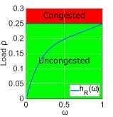
(a) $R=4$

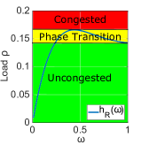
(b) $R=7$

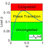
(c) $R=10$

Figure 15: Illustration of the different network regimes for different values of $R$. For each value of $\rho$, the fixed points are the solutions of $h_{R}(\omega)=\rho$. In addition, the fixed point $\omega=1$ always exists when $\rho>1/R$. A phase transition region exists if the maximum of $h_{R}(\omega)$, $h_{R}^{max}$, is strictly greater than $h_{R}(1)=1/R$.

V-E Sufficient condition for phase transition

In the previous section, we showed that a phase transition exists in the region $1/R<\rho<h^{max}_{R}$, if $h^{max}_{R}>1/R$. In this section, we derive an explicit lower bound on $h^{max}_{R}$, which provides a simple condition for the existence of a phase transition. First, we establish a relationship between the derivatives of $h_{R}(\omega)$ for different values of $R$, but a given value of $\omega$.

Lemma 3

For $\omega\in[0,1]$, if there exists $R^{*}\geq 1$ such that $h_{R^{*}}^{\prime}(\omega)\leq 0$, then $h_{R}^{\prime}(\omega)\leq 0$ for all $R>R^{*}$.

Proof:

Let $\omega\in[0,1]$. Since

$$\left(h_{R}^{-1}(\omega)\right)^{\prime}=-\frac{h_{R}^{\prime}(\omega)}{h_{R}(\omega)^{2}},$$ (21)

the sign of $h_{R}^{\prime}(\omega)$ is opposite to $\left(h_{R}^{-1}(\omega)\right)^{\prime}$. Hence, we investigate the sign of

$$\left(h_{R}^{-1}(\omega)\right)^{\prime}=\sum_{r=1}^{R}\Psi_{r}^{\prime}(\omega),$$ (22)

where

$$\Psi_{r}(\omega)\triangleq\frac{\left(1-\mathrm{e}^{-\omega}(1-\omega)\right)^{r-1}}{\omega}.$$ (23)

We check the sign of each term $\Psi_{r}^{\prime}(\omega)$ in (22), for $r\in\{1,2,\ldots,R\}$. For $r=1$, we have

$$\Psi_{1}^{\prime}(\omega)=\frac{d}{d\omega}\left(\frac{1}{\omega}\right)=-\frac{1}{\omega^{2}}<0.$$

For $r\geq 2$, we have

$$\Psi_{r}^{\prime}(\omega)=-\frac{e^{-\omega}\left(1-\mathrm{e}^{-\omega}(1-\omega)\right)^{r-2}\Phi_{r}(\omega)}{\omega^{2}},$$ (24)

where

$$\Phi_{r}(\omega)\triangleq-1+e^{\omega}+(3-2r)\omega+(r-1)\omega^{2}.$$

Clearly, the terms $e^{-\omega}$, $\left(1-\mathrm{e}^{-\omega}(1-\omega)\right)^{r-2}$ and $\omega^{2}$ in (24) are all positive. Thus, the signs of $\Phi_{r}(\omega)$ and $\Psi_{r}^{\prime}(\omega)$ are opposite.

We next investigate the signs of the first and second derivatives of the function $\Phi(\omega)$. We have

$$\Phi_{r}^{\prime}(\omega) = e^{\omega}+3-2r+2(r-1)\omega,$$ (25)

$$\Phi_{r}^{\prime\prime}(\omega) = e^{\omega}+2(r-1)>0,$$ (26)

for all $\omega\in[0,1]$ and $r\geq 2$. From (26), we find that $\Phi_{r}^{\prime}(\omega)$ is monotonically increasing with $\omega$.

For any $r\geq 2$, we obtain from (25) that

$$\Phi_{r}^{\prime}(0) = 4-2r,$$ (27)

$$\Phi_{r}^{\prime}(1) = e+1.$$ (28)

We distinguish between three possible cases regarding the sign of $\Phi_{r}(\omega)$:

1. For $r=2$, $\Phi_{2}^{\prime}(0)=0$. Hence, $\Phi_{2}^{\prime}(\omega)>0$. The function $\Phi_{2}(\omega)$ is monotonically increasing with $\omega$. Since $\Phi_{2}(0)=e-1>0$, $\Phi_{2}(\omega)$ is always positive.

2. For $r=3$, $\Phi_{3}^{\prime}(0)<0$. The function $\Phi_{3}(\omega)$ first decreases then increases as $\omega$ increases from 0 to 1. Since $\Phi_{3}(0)=0$ and $\Phi_{3}(1)>0$, the sign of the function $\Phi_{3}(\omega)$ turns from negative to positive as $\omega$ increases from $0$ to $1$.

3. For $r>3$, $\Phi_{r}^{\prime}(0)<0$. The function $\Phi_{r}(\omega)$ first decreases then increases as $\omega$ increases from 0 to 1. Since $\Phi_{r}(0)=0$ and $\Phi_{r}(1)<0$, the sign of the function $\Phi_{r}(\omega)$ is always negative.

Therefore, by (22), for any given $\omega\in[0,1]$, the sign of the function $\Phi_{r}(\omega)$ turns from being positive to being negative as $r$ increases. Equivalently, the sign of the function $\Psi_{r}^{\prime}(\omega)$ turns from being negative to being positive as $r$ increases.

Thus, by (22), if $\left(h_{R}^{-1}(\omega)\right)^{\prime}$ is nonnegative for $R=R^{*}$, then it is also nonnegative for all $R\geq R^{*}$. Equivalently, by (21), if $\left(h_{R}^{-1}(\omega)\right)^{\prime}$ is nonpositive for $R=R^{*}$, then it is also nonpositive for all $R\geq R^{*}$, which completes the proof. ∎

Consider the function $h_{R}(\omega)$ as $R\rightarrow\infty$:

$$h_{\infty}(\omega) = (1-\left(1-\mathrm{e}^{-\omega}(1-\omega)\right))\omega$$ (29)

$$= e^{-\omega}(1-\omega)\omega,$$

and its derivative

$$h_{\infty}^{\prime}(\omega)=e^{-\omega}(1-3\omega+\omega^{2}).$$ (30)

The next corollary is the logical transposition of Lemma 3.

Corollary 1

If $h_{\infty}^{\prime}(\omega)\geq 0$, then $h_{R}^{\prime}(\omega)\geq 0$ for all $R\geq 1$.

The following lemma establishes that the function $h_{R}(\omega)$ is always strictly increasing in the interval $[0,\overline{\omega})$, where

$$\overline{\omega}\triangleq\frac{3-\sqrt{5}}{2}.$$ (31)

Lemma 4

Let $0\leq\omega<\overline{\omega}$. Then, $h_{R}^{\prime}(\omega)>0$, for all $R\geq 1$.

Proof:

Let the function $h_{\infty}(\omega)$ and its derivative $h_{\infty}^{\prime}(\omega)$ be defined as in (29) and (30), respectively. Since $e^{-\omega}$ is always positive, $h_{\infty}^{\prime}(\omega)$ has the same sign as $(1-3\omega+\omega^{2})$. The unique root of $(1-3\omega+\omega^{2})=0$ for $\omega\in[0,1]$ is $\bar{w}$ as defined in (31).

Thus, $(1-3\omega+\omega^{2})$ is positive when $0\leq\omega<\overline{\omega}$, and so is $h_{\infty}^{\prime}(\omega)$. By Corollary 1, $h_{R}^{\prime}(\omega)>0$ for $0\leq\omega<\overline{\omega}$ and for all $R\geq 1$.

∎

The consequence of Lemma 4 is that for all $R\geq 1$,

$$h^{max}_{R}\geq h_{R}(\overline{\omega}).$$ (32)

This equation provide a lower bound on $h^{max}_{R}$ that can easily be computed. We then obtain the following sufficient condition for the existence of phase transition.

Theorem 3

Let $\overline{\omega}$ be defined as in (31) and suppose $h_{R}(\overline{\omega})>1/R$. Then, a phase transition is guaranteed to exist for any $\rho\in(1/R,h_{R}(\overline{\omega}))$.

Proof:

From Theorem 2, we know that a phase transition exists if $1/R<\rho<h^{max}_{R}$. By (32) and the assumption that $h_{R}(\overline{\omega})>1/R$, the proof follows. ∎

The next theorem establishes an even more explicit lower bound on $h^{max}_{R}$.

Theorem 4

Let $h_{\infty}(\omega)$ and $\overline{\omega}$ be defined as in (29) and (31), respectively. Then, $h^{max}_{R}\geq h_{\infty}(\overline{\omega})\simeq 0.161$.

Proof:

By (19),

$$h_{R}(\overline{\omega}) = \frac{\omega}{\sum_{r=1}^{R}(1-e^{-\omega}(1-\omega))^{r-1}}$$ (33)

$$> \frac{\omega}{\sum_{r=1}^{\infty}(1-e^{-\omega}(1-\omega))^{r-1}}=h_{\infty}(\overline{\omega}).$$

Thus, by (32) and  (33), $h^{max}_{R}>h_{\infty}(\overline{\omega})\simeq 0.161$. Note that this bound is asymptotically tight as $R\to\infty$ since $h^{max}_{\infty}=h_{\infty}(\overline{\omega})$. ∎

From Theorems 2 and 4, it follows that a phase transition exists if $1/R<0.161$. Hence:

Corollary 2

A phase transition is guaranteed to exist for $R\geq 7$ and $\rho\in[1/R,0.161]$.

We note that the lower bound on $h^{max}_{R}$ is quite tight. For instance, $h^{max}_{7}=0.166$. Moreover, $h^{max}_{R}$ decreases with $R$ (this follows from (19), since for any $\omega\in[0,1]$ the denominator increases as $R$ gets larger).

V-F Stability of fixed points

In this subsection, we use stability theory to shed further light into the limiting behaviour of the sequence $(u_{i})_{i=0}^{\infty}$. Specifically, the sequence $(u_{i})_{i=0}^{\infty}$ converges to stable fixed points of $\Omega$ and diverges from unstable fixed points of $\Omega$. We will show that the stability of the fixed points of (18) are determined by the sign of $h_{R}^{\prime}(\omega)$ at those points.

Informally, a fixed point $\omega$ is stable (or an attractor), if there exists a domain containing $\omega$, such that if $u_{0}$ belongs to that domain, then $(u_{i})_{i=0}^{\infty}$ converges to $\omega$.

Definition 3 (Stability of a fixed point)

Let $u_{0}\in[0,1]$. A fixed point $\omega\in\Omega$ is stable if there exists $\epsilon>0$ such that if $|u_{0}-\omega|<\epsilon$, the sequence $(u_{i})_{i=0}^{\infty}$ converges to $\omega$. It is unstable if for all $u_{0}\neq\omega$ the sequence $(u_{i})_{i=0}^{\infty}$ does not converge to $\omega$.

Recall that according to Lemma 2, a special fixed point of (15) exists at $\omega=1$, if $\rho>1/R$. According to Definition 3, this fixed point is stable. Besides this special case, the rest of the fixed points satisfy Equation (18). To establish the stability of those fixed points, we will employ the following proposition.

Proposition 1 ([39])

Suppose that a continuously differentiable function $f$ has a fixed point $\omega$. Then, $\omega$ is stable if $|f^{\prime}(\omega)|<1$ and unstable if $|f^{\prime}(\omega)|>1$.

The next theorem provides a criterion to establish the stability of a fixed point $\omega\in\Omega$ with respect to the function $h_{R}(\omega)$.

Theorem 5

Consider a fixed point $\omega\in\Omega$, where $\omega<1$. Then $\omega$ is stable if $h_{R}^{\prime}(\omega)>0$ and unstable if $h_{R}^{\prime}(\omega)<0$.

Proof:

Let $\omega\in\Omega$. The derivative of $h_{R}(\omega)$ with respect to $\omega$ is

$$h_{R}^{\prime}(\omega)=\frac{1}{\Gamma(\omega)}-\frac{\omega}{(\Gamma(\omega))^{2}}\cdot\Gamma^{\prime}(\omega)>0,$$ (34)

where

$$\Gamma(\omega)\triangleq\sum_{r=1}^{R}\left(1-\mathrm{e}^{-\omega}(1-\omega)\right)^{r-1}=\frac{f(\omega)}{\rho}.$$ (35)

If one can show that (34) implies $|f^{\prime}(\omega)|<1$, then according to Proposition 1, the fixed point $\omega$ is stable. We multiply both sides of (34) by $(\Gamma(\omega))^{2}$ and obtain

$$\Gamma(\omega)-\omega\Gamma^{\prime}(\omega)>0.$$ (36)

Using (35) and (18), we can rearrange (36) as follows:

$$\Gamma^{\prime}(\omega)<\frac{\Gamma(\omega)}{\omega}=\frac{f(\omega)}{\rho\omega}=\frac{1}{\rho}.$$ (37)

From (35) and (37), we get

$$f^{\prime}(\omega)=\rho\Gamma^{\prime}(\omega)<1.$$

Since $f(\omega)$ is monotonically increasing with $\omega$, for $\omega\in[0,1]$, we conclude

$$0<f^{\prime}(\omega)<1.$$

Hence, by Proposition 1, $\omega$ is a stable fixed point.

Similarly, $h_{R}^{\prime}(\omega)<0$ implies $f^{\prime}(\omega)>1$, which means that $\omega$ is unstable.

∎

We next show how the stability analysis of the fixed points helps to determine the limit of the sequence $(u_{i})_{i=0}^{\infty}$. Consider, for instance, the example shown in Figure 16 with parameters $R=10$ and $\rho=0.13$. Under these parameters, $\Omega=\{\omega_{1},\omega_{2},\omega_{3}\}=\{0.2,0.7,1\}$.

The fixed points $\omega_{1}$ and $\omega_{2}$ are the solutions of $h_{R}(\omega)=\rho$. According to Theorem 5, $\omega_{1}$ is stable and $\omega_{2}$ is unstable. The fixed point $\omega_{3}=1$ exists and is stable, since $\rho>1/R$.

According to Theorem 2, $\omega_{2}$ is a phase transition point. Hence, the sequence $(u_{i})_{i=0}^{\infty}$ converges to $\omega_{1}$ if $u_{0}<\omega_{2}$ and the network is uncongested. If $u_{0}>\omega_{2}$, the sequence converges to $\omega_{3}$ and the network is congested.

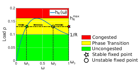
Figure 16: Stability of fixed points with $R=10$. Given a load $\rho=0.13$ (dash line), $\Omega$ contains three fixed points: $\omega_{1}=0.2$, $\omega_{2}=0.7$ and $\omega_{3}=1$. The fixed point $\omega_{1}$ is stable because $h^{\prime}_{R}(\omega_{1})>0$ and $\omega_{2}$ is unstable because $h^{\prime}_{R}(\omega_{2})<0$. The fixed point $\omega_{3}=1$ exists and is stable because $\rho>1/R$. Therefore, the sequence $(u_{i})_{i=0}^{\infty}$ converges to $\omega_{1}$ if $u_{0}<\omega_{2}$, and to $\omega_{3}$ if $u_{0}>\omega_{2}$.

V-G Heterogeneous traffic load

In previous subsections, we assumed that node $A_{0}$ varies its traffic load $\rho_{0}$, but all other nodes $A_{i}$ ($i\geq 1$) have the same traffic load $\rho$. We now relax this assumption and assume that nodes $A_{i}$ ($i\geq 1$) have different traffic loads $\rho_{i}=\lambda_{i}T$. We next prove that a phase transition still occurs, as long as all the traffic loads fall in the appropriate range.

Theorem 6

Suppose $h^{max}_{R}>1/R$. If $\rho_{i}\in(1/R,h^{max}_{R})$ for all $i\geq 1$, then a phase transition occurs.

Proof:

Let $\rho_{max}=\max_{i\geq 1}\rho_{i}$ and $\rho_{min}=\min_{i\geq 1}\rho_{i}$. According to Theorem 2, the network is uncongested when $\rho_{0}=0$ and the load at each node $A_{i}$ is $\rho_{max}<h_{R}^{max}$. Hence, the network must remain uncongested when the load at each node $A_{i}$ is smaller than $\rho_{max}$.

Similarly, the network is congested when $\rho_{0}=1$ and the load at each node $A_{i}$ is $\rho_{min}>1/R$. Hence, it must remain congested when the load at each node $A_{i}$ is larger than $\rho_{min}$. Thus, a phase transition occurs when $1/R<\rho_{i}<h_{R}^{max}$ for all $i\geq 1$. ∎

V-H Comparison with simulation results

We compare the results of our analysis with ns-3 simulations, for different settings of the retry limit $R$ and load $\rho$. For the simulations, we consider an ad hoc network composed of 41 pairs of nodes, as described in Section IV-B1.

V-H1 Region of phase transition

To check whether a phase transition exists for a given $R$, we run simulations both for $\rho_{0}=0$ and $\rho_{0}=1$. If the node utilizations in the limit (i.e., for node $A_{40}$) is the same in both cases, then we assume that there is no phase transition. If the limits are different, then a phase transition exists.

Figure 17 indicates that the existence of a phase transition is related to the retry limit, as predicted by our analysis. For the case $R=4$, there is no phase transition, while a phase transition occurs in the cases $R=7$ and $R=10$. in our simulations for any $R\leq 6$.

The analysis also reasonably approximates the phase transition region. For $R=7$, the simulations show that a phase transition exists if $\rho\in(0.12,0.16)$, while the analysis predicts $\rho\in(0.14,0.17)$. For $R=10$, the simulation results are $\rho\in(0.08,0.14)$ while the analysis predicts $\rho\in(0.10,0.16)$. We note that the size of the phase transition region increases with $R$, as predicted by the analysis.

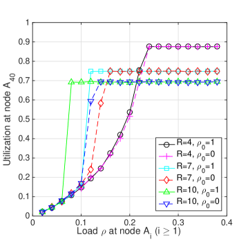
Figure 17: Simulation of the limiting behaviour of the node utilization in a network of 41 pairs of nodes. For $R=4$, the limit is the same when $\rho_{0}=0$ and $\rho_{0}=1$, hence no phase transition is observed. However, for $R=7$ and $R=10$, the limits are different, hence showing the existence of a region of load $\rho$ in which a phase transition occurs.

V-H2 Heterogeneous traffic load

We next show the feasibility of a cascading DoS attack in a network where the traffic load at different node is heterogeneous, in line with the analysis of Section V-G. Specifically, the traffic load $\rho_{i}$ at each node $A_{i}$ ($i\geq 1$) is a continuous random variable that is uniformly distributed between 0.11 and 0.15.

Figure 18 shows the simulation results for retry limit $R=7$. When $\rho_{0}$, the load of node $A_{0}$, is below 0.5, the network is uncongested and the utilizations of nodes $A_{i}$ oscillate around 0.35 as $i$ gets large. Note that the sequence does not converge to a fixed value due to the different traffic loads at the different nodes. However, when $\rho_{0}$ exceeds 0.6, the sequence of node utilizations converges to its upper limit, implying that the network is congested.

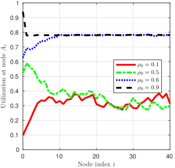
Figure 18: Simulation with heterogeneous traffic load in a network with 41 pairs of nodes. The traffic load of nodes $A_{i}$ ($i\geq 1$) are uniformly distributed between 0.11 and 0.15. For $R=7$, when the load $\rho_{0}$ changes from 0.5 to 0.6, the limiting behavior of the sequence of node utilizations differs, thus indicating the occurrence of phase transition.

VI Conclusion

We describe a new type of DoS attacks against Wi-Fi networks, called cascading DoS attacks. The attack exploits a coupling vulnerability due to hidden nodes. The attack propagates beyond the starting location, lasts for long periods of time, and forces the network to operate at its lowest bit rate. The attack can be started remotely and without violating the IEEE 802.11 standard, making it difficult to trace back.

We demonstrate the feasibility of such attacks, both through experiments on a testbed and extensive ns-3 simulations. The simulations show that the attack is effective in networks operating under fixed and varying bit rates, as well as ad hoc and infrastructure modes. We show that a small change in the traffic load of the attacker can lead to a phase transition of the entire network, from uncongested state to congested state.

We develop an iterative analysis to characterize the sequence of node utilizations, and study its limiting behaviour. We show that the sequence always converges to stable fixed points while an unstable fixed point represents a phase transition point. Based on the system parameters, we identify when the system remains always uncongested, congested, or experiences a phase transition caused by a DoS cascading attack.

The analysis predicts that a phase transition occurs for $R\geq 7$ and provides a simple and explicit estimate of traffic load at each node under which a phase transition occurs (i.e., $\rho_{i}\in(1/R,0.161)$ for all $i\geq 1$). The network is always congested when the traffic load is above the phase transition regime and always uncongested when the traffic load is below the phase transition regime. Although the analysis is based on some simplifying assumptions, the estimate is not far from the values observed in the simulations.

Exploiting the coupling vulnerability in different network configurations represents an interesting area for future work. Experience in the security field indeed teaches that once a vulnerability is identified, more potent attacks are subsequently discovered (consider, for instance, the history of attacks on WEP [40] and MD5 [41]). In our case, our simulations for ring topologies indicate that the presence of a cycle in the topology could reinforce cascading DoS attacks, a result that warrants further investigations.

Several approaches are possible to mitigate cascading DoS attacks. First, one could enable the RTS/CTS exchange, although this solution has several drawbacks, including major performance degradation under normal network operations, as mentioned in the Introduction. Devising a scheme that triggers RTS/CTS under certain circumstances (e.g., multiple consecutive packet losses) could be an interesting area for future research. The second approach is to lower the retry limit. However, this could also negatively impact performance. Other approaches include using short packets, collision-aware rate adaptation algorithms, dynamic channel selection, and full-duplex radios. We leave the investigation and comparison of these mitigation techniques as possible areas for future work.

References

- [1] K. Lee, J. Lee, Y. Yi, I. Rhee, and S. Chong, “Mobile data offloading: how much can WiFi deliver?” in Proceedings of the 6th International Conference on emerging Networking EXperiments and Technologies (CoNEXT). ACM, 2010, p. 26.
- [2] Cisco, “Cisco cleanair technology,” http://www.cisco.com/c/en/us/solutions/enterprise-networks/cleanair-technology/index.html.
- [3] G. Bianchi, “Performance analysis of the IEEE 802.11 distributed coordination function,” IEEE Journal on Selected Areas in Communication, vol. 18, no. 3, pp. 535–547, 2000.
- [4] A. Forouzan Behrouz, Data Communication and Networking. 3rd/4th Edition, Tata McGraw, 2004.
- [5] M. Gast, 802.11 wireless networks: the definitive guide. O’Reilly Media, Inc., 2005.
- [6] http://documentation.netgear.com/WPN824EXT/enu/202-10310-02/WPN824EXT_UG-4-6.html.
- [7] http://www.tp-link.us/support/download-center.
- [8] http://ui.linksys.com/WAG300N/1.01.01/help/h_AdvWSettings.htm.
- [9] http://support.dlink.com/emulators/dir855/Advanced.html.
- [10] V. Saligrama and D. Starobinski, “On the macroscopic effects of local interactions in multi-hop wireless networks,” in Modeling and Optimization in Mobile, Ad Hoc and Wireless Networks, 2006 4th International Symposium on. IEEE, 2006.
- [11] L. Xin, D. Starobinski, and G. Noubir, “Cascading denial of service attacks on Wi-Fi networks,” in Communications and Network Security (CNS), 2016 IEEE Conference.
- [12] R. Poisel, Modern communications jamming principles and techniques. Artech House Publishers, 2011.
- [13] K. Pelechrinis, M. Iliofotou, and S. V. Krishnamurthy, “Denial of service attacks in wireless networks: The case of jammers,” Communications Surveys & Tutorials, IEEE, vol. 13, no. 2, pp. 245–257, 2011.
- [14] G. Lin and G. Noubir, “On link layer denial of service in data wireless LANs,” Wireless Communications and Mobile Computing, vol. 5, no. 3, pp. 273–284, 2005.
- [15] G. Noubir, R. Rajaraman, B. Sheng, and B. Thapa, “On the robustness of IEEE 802.11 rate adaptation algorithms against smart jamming,” in Proceedings of the fourth ACM conference on Wireless network security. ACM, 2011, pp. 97–108.
- [16] C. Orakcal and D. Starobinski, “Jamming-resistant rate adaptation in Wi-Fi networks,” Performance Evaluation, vol. 75, pp. 50–68, 2014.
- [17] C. Chen, H. Luo, E. Seo, N. H. Vaidya, and X. Wang, “Rate-adaptive framing for interfered wireless networks,” in INFOCOM 2007. 26th IEEE International Conference on Computer Communications. IEEE.
- [18] S. Rayanchu, A. Mishra, D. Agrawal, S. Saha, and S. Banerjee, “Diagnosing wireless packet losses in 802.11: Separating collision from weak signal,” in INFOCOM 2008. The 27th Conference on Computer Communications. IEEE.
- [19] “Minstrel madwifi documentation,” http://linuxwireless.org/en/developers/Documentation/mac80211/RateControl/minstrel.
- [20] R. Kinney, P. Crucitti, R. Albert, and V. Latora, “Modeling cascading failures in the north american power grid,” The European Physical Journal B-Condensed Matter and Complex Systems, vol. 46, no. 1, pp. 101–107, 2005.
- [21] S. Soltan, D. Mazauric, and G. Zussman, “Cascading failures in power grids: analysis and algorithms,” in Proceedings of the 5th international conference on Future energy systems. ACM, 2014, pp. 195–206.
- [22] M. Haenggi, J. G. Andrews, F. Baccelli, O. Dousse, and M. Franceschetti, “Stochastic geometry and random graphs for the analysis and design of wireless networks,” Selected Areas in Communications, IEEE Journal on, vol. 27, no. 7, pp. 1029–1046, 2009.
- [23] Z. Kong and E. M. Yeh, “Wireless network resilience to degree-dependent and cascading node failures,” in Modeling and Optimization in Mobile, Ad Hoc, and Wireless Networks, 2009. WiOPT 2009. 7th International Symposium on. IEEE, 2009.
- [24] A. Aziz, D. Starobinski, P. Thiran, and A. El Fawal, “EZ-Flow: Removing turbulence in IEEE 802.11 wireless mesh networks without message passing,” in Proceedings of the 5th International Conference on Emerging Networking Experiments and Technologies (CoNEXT). ACM, 2009, pp. 73–84.
- [25] A. Aziz, D. Starobinski, and P. Thiran, “Understanding and tackling the root causes of instability in wireless mesh networks,” IEEE/ACM Transactions on Networking, vol. 19, no. 4, pp. 1178–1193, 2011.
- [26] S. Ray, D. Starobinski, and J. B. Carruthers, “Performance of wireless networks with hidden nodes: a queuing-theoretic analysis,” Computer Communications, vol. 28, no. 10, pp. 1179–1192, 2005.
- [27] S. Ray, J. B. Carruthers, and D. Starobinski, “Evaluation of the masked node problem in ad hoc wireless LANs,” Mobile Computing, IEEE Transactions on, vol. 4, no. 5, pp. 430–442, 2005.
- [28] S. Ray and D. Starobinski, “On false blocking in RTS/CTS-based multihop wireless networks,” Vehicular Technology, IEEE Transactions on, vol. 56, no. 2, pp. 849–862, 2007.
- [29] J. Bellardo and S. Savage, “802.11 denial-of-service attacks: Real vulnerabilities and practical solutions.” in USENIX security, 2003, pp. 15–28.
- [30] J. C. Stein, “Indoor radio WLAN performance part II: Range performance in a dense office environment,” Intersil Corporation, vol. 2401, 1998.
- [31] “iperf 2 user documentation,” http://iperf.fr/iperf-doc.php.
- [32] D. Xia, J. Hart, and Q. Fu, “Evaluation of the minstrel rate adaptation algorithm in IEEE 802.11g WLANs,” in 2013 IEEE International Conference on Communications (ICC).
- [33] https://www.nsnam.org/doxygen/classns3_1_1_ap_wifi_mac.html#details.
- [34] https://www.nsnam.org/doxygen/classns3_1_1_sta_wifi_mac.html#details.
- [35] https://www.nsnam.org/doxygen/classns3_1_1_hybrid_buildings_propagation_loss_model.html#details.
- [36] B. Rong and A. Ephremides, “Protocol-level cooperation in wireless networks: Stable throughput and delay analysis,” in Modeling and Optimization in Mobile, Ad Hoc, and Wireless Networks, 2009. WiOPT 2009. 7th International Symposium on. IEEE, 2009.
- [37] L. Kleinrock, F. Tobagi et al., “Packet switching in radio channels: Part I–carrier sense multiple-access modes and their throughput-delay characteristics,” Communications, IEEE Transactions on, vol. 23, no. 12, pp. 1400–1416, 1975.
- [38] D. Bertsekas and R. Gallager, “Data networks. 1992,” PrenticeHall, Englewood Cliffs, NJ, 1992.
- [39] S. Lynch, Dynamical systems with applications using MATLAB. Springer, 2004.
- [40] E. Tews, R.-P. Weinmann, and A. Pyshkin, “Breaking 104 bit WEP in less than 60 seconds,” in Information Security Applications. Springer, 2007, pp. 188–202.
- [41] J. Black, M. Cochran, and T. Highland, “A study of the MD5 attacks: Insights and improvements,” in Fast Software Encryption. Springer, 2006, pp. 262–277.