Thermodynamic optimization of an electric circuit as a non–steady energy converter

Abstract

Electrical circuits with transient elements can be good examples of systems where non–steady irreversible processes occur, so in the same way as a steady state energy converter, we use the formal construction of the first order irreversible thermodynamic (FOIT) to describe the energetics of these circuits. In this case, we propose an isothermic model of two meshes with transient and passive elements, besides containing two voltage sources (which can be functions of time); this is a non–steady energy converter model. Through the Kirchhoff equations, we can write the circuit phenomenological equations. Then, we apply an integral transformation to linearise the dynamic equations and rewrite them in algebraic form, but in the frequency space. However, the same symmetry for steady states appears (cross effects). Thus, we can study the energetic performance of this converter model by means of two parameters: the “force ratio” and the “coupling degree”. Furthermore, it is possible to obtain the characteristic functions (dissipation function, power output, efficiency, etc.). They allow us to establish a simple optimal operation regime of this energy converter. As an example, we obtain the converter behavior for the maximum efficient power regime (MPE).

Keywords: Non–Equilibrium and irreversible thermodynamics; Performance characteristics of energy conversion systems; figure of merit; Energy conversion.

1 Introduction

The development of Non–Equilibrium Thermodynamics has several objectives, these objectives go from determining the properties of materials [1, 2, 3] under different gradients to testing the consistency of the cosmological models [4, 5, 6]. One of these objetives, which is at the same time a kind of tool, gives rise to the study of energy conversion. The energy performance of the converters can be studied based on the entropy production. Using the form of this quantity we can construct the functions that characterize its energetic performance [7, 8]. In particular, in a linear and steady regime one finds that the energy performance obeys operating regimes consistent with imposed boundary conditions; these conditions imply specific relations among its design and the spontaneous and non–spontaneous gradients on the system [9, 10, 11]. The optimal points of operation are related with the boundary conditions and are linked with several optimization criteria (objective functions) independent from the model. A model with these features, can be used to describe actual converters [11, 12]. Nevertheless, it is clear that real processes occur in non–steady conditions, so it is essential to develop a basic model for these conditions (see Figure 1).

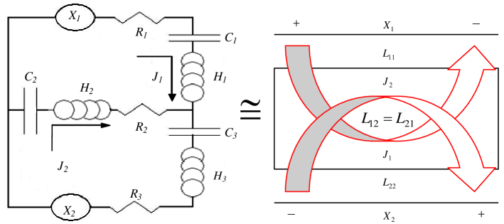
Figure 1: LCR–circuit of two meshes as an energy converter model (left) can be depicted with the scheme on the right side, which is the simplest energy converter (two fluxes and two forces). Through the expresion for the entropy production: $\sigma=J_{1}X_{1}+J_{2}X_{2}>0$ and direction of fluxes, we regard that $\left|J_{2}X_{2}\right|>\left|J_{1}X_{1}\right|$ where $X_{1}<0$ is linked with non–spontaneous flux, while $X_{2}>0$ causes the spontaneous flux.

From the Caplan and Essig works [13], one can make a first step toward a description of linear energy converters with two coupled fluxes and two forces. In general the flows $J_{i}$ displayed on a real system are usually complicated non–linear functions of the forces $X_{i}$. However, the linear regime allows us to give a quite acceptable description of the phenomenon of energy conversion. The phenomenological equations of this system are given by

$$J_{1}=L_{11}X_{1}+L_{12}X_{2}$$ (1)

and

$$J_{2}=L_{21}X_{1}+L_{22}X_{2},$$ (2)

where $L_{ij}=\left(\nicefrac{{\partial J_{i}}}{{\partial X_{i}}}\right)_{eq}$ are the partial derivatives evaluated at equilibrium, called the phenomenological coefficients. Furthermore, if it is admitted at this point the Onsager reciprocal relationship between the phenomenological cross coefficients, $L_{12}=L_{21}$. Then we can describe the process of energy conversion of this basic model in the easiest way.

From this linear scheme (Eqs. 1 and 2), Kadem and Caplan have introduced the degree of coupling

$$q^{2}=\frac{L_{12}^{2}}{L_{11}L_{22}}\geq 0.$$ (3)

This is a dimensionless paratemer which measures the quality of the coupling between spontaneous and non–spontaneous fluxes and comes directly from the thermodynamics’ second law (Figure 1) [10, 13]. On the other hand, following the paper published by Stucki [14], it is suitable to take again the definition of the force ratio, given by [15]

$$x=\sqrt{\frac{L_{11}}{L_{22}}}\frac{X_{1}}{X_{2}}=\sqrt{\frac{L_{11}}{L_{22}}}x^{\prime},$$ (4)

which measures a direct relationship between the two forces through $x^{\prime}$, we call $x^{\prime}=\left(\nicefrac{{X_{1}}}{{X_{2}}}\right)$ the force quotient. Moreover, in Sec. 2.1 we will be able to write (1) and (2) in terms of the $q$ and $x$ parameters, although we admit that phenomenological equations show time dependence.

One of these converters, which can be studied in a regime dependent on time with a good approximation is an electric circuit with transient elements, such as capacitors and inductors. The dynamic behavior of these elements is well–known, and secondly, we know that optimization criteria do not depend on the model. Then it is possible to build a non–steady circuit, i.e, one that contains both capacitors and inductors in order to study its energetic performance. In this paper (section 2) we have considered an inductive–capacitive–resistive (LCR) circuit of two meshes, that works through voltage sources which may even depend on time. In this way the corresponding phenomenological relationships also depend on time. Due to these equations not being inverted easily, we should apply a suitable integral transformation, then they turn algebraic in the frequency space. When we return to the time space by a reverse transformation, the inverted generalized equations satisfy the same reciprocal relationships as well as steady converters [16]. For this reason, this LCR circuit can be described using the same model presented in [10]. Now we have phenomenological coefficients space time dependent, which contain information about charging and saturation time of transient elements in the circuit.

In section 3 we will discuss the energetic behavior of this $(2\times 2)$ converter, being that it can work in several operation well–known regimes (minimum dissipation, maximum power output, maximum efficiency, maximum ecological function, etc.) [10, 12, 17]. Additionally, we study the evolution of some characteristic functions when voltage sources are constant and when they depend periodically on time, in some of the above regimes. With the same objetive, in section 4 we focus our attention on another operation regime, which was derived from the optimization criterion called “Efficient Power” proposed by Sucki to study the energetics of the mithochondria [14] and used by Yilmaz in the context of Finite Time Thermodynamics (FFT) [18]. In this section we establish and discuss this mode of operation for the LCR circuit. Finally, in section 5 we write some conclusions based in our results.

2 Energetics of LCR–circuit as a converter with two coupled fluxes

In this section we estudy the energetics of a $(2\times 2)$ system through the constitutive equations dependent on the time. By means of the quantities $\left(q,x\right)$ we write their characteristic functions and shall obtain their temporal evolution. This evolution is possible because the circuit depends on the nature of the transient elements and due to the fact $L_{12}(t)=L_{21}(t)$, then we can establish some optimum modes of operation.

2.1 Constitutive equations

Let $J_{1}=J_{1}(t)$ and $J_{2}=J_{2}(t)$ be the same two coupled generalized fluxes ($J_{1}$ being the driven flux and $J_{2}$ the driver flux) which appear in the description of steady energy converters; besides $X_{1}$ and $X_{2}$ are the conjugate generalized forces associated with the fluxes. For the linear regime, fluxes depend on the forces by means the Onsager equations. Therewith, if we use the parameters of design and mode of operation defined by (3) and (4) we can rewrite (5) and (6) as:

$$J_{1}=\sqrt{L_{11}}\left(X_{1}\sqrt{L_{11}}+X_{2}\sqrt{L_{22}}q\right)=\left(\frac{x+q}{x}\right)L_{11}X_{1},$$ (5)

$$J_{2}=\sqrt{L_{22}}\left(X_{1}\sqrt{L_{11}}q+X_{2}\sqrt{L_{22}}\right)=\left(1+qx\right)L_{22}X_{2},$$ (6)

where $\left(L_{12}=L_{21}\right)$, the Onsager symmetry relation between crossed coefficients has been used. We note that in the limit case $q\rightarrow 0$, each flux becomes proportional to its proper conjugate force through the direct phenomenological coefficient, i.e, cross effects vanish and therefore the fluxes become independent. And when $q\rightarrow 1$, the fluxes tend to a fixed relationship independently of the magnitudes force [10, 13]. Here we have taken $X_{2}>0$ as the associated force to the driver flux. Whereby, $x$ measures the fraction of $X_{1}<0$ appearing due to the presence of the flux $J_{2}$. Then, the physical values for the force ratio parameter are in the interval $\left[-1,0\right]$. We also can represent $J_{1}$ and $J_{2}$, if we know the force $X_{2}$, which is carried out in pro the gradient. Henceforth, energy convertion description will be expressed with this condition.

2.2 LCR–circuit’s dynamic equations

In the LCR–circuit (see Figure 1) there are two coupled fluxes (currents) and two conjugate forces (voltages). The phenomenological equations of the circuit are given by the Kirchhoff laws; if we apply the corresponding Kirchhoff equation (energy conservation), for the mesh 1 (left side) we have:

$$X_{1}=\left(\frac{1}{C_{1}}+\frac{1}{C_{2}}\right)\int J_{1}dt+\left(H_{1}+H_{2}\right)\frac{dJ_{1}}{dt}+\left(R_{1}+R_{2}\right)J_{1}-\frac{1}{C_{2}}\int J_{2}dt-H_{2}\frac{dJ_{2}}{dt}-R_{2}J_{2},$$ (7)

while for the mesh 2 (right side) the equation is:

$$X_{2}=\left(\frac{1}{C_{2}}+\frac{1}{C_{3}}\right)\int J_{2}dt+\left(H_{2}+H_{3}\right)\frac{dJ_{2}}{dt}+\left(R_{2}+R_{3}\right)J_{2}-\frac{1}{C_{2}}\int J_{1}dt-H_{2}\frac{dJ_{1}}{dt}-R_{2}J_{1}.$$ (8)

Hereafter, we have considered that the inductors are far enough apart to neglet the effect of mutual inductances.

2.2.1 Direct Current LCR system

First, we consider $X_{1}$ and $X_{2}$ independent on time, then we note that (7) and (8) are not simple invertible equations. So, we can use an integral transformation (Laplace transformation) because it enables direct inclusion of initial conditions for the circuit. Hence, the above equations are sent to the frequency space and they become invertible equations:

$$\frac{X_{1}}{s}=\left(\frac{1}{C_{1}}+\frac{1}{C_{2}}\right)\frac{I_{1}(s)}{s}+\frac{q_{0}}{sC_{1}}+s\left(H_{1}+H_{2}\right)I_{1}(s)-H_{1}J(0+)+\left(R_{1}+R_{2}\right)I_{1}(s)-\frac{I_{2}(s)}{sC_{2}}-sH_{2}I_{2}(s)-R_{2}I_{2}(s),$$ (9)

and

$$\frac{X_{2}}{s}=\left(\frac{1}{C_{2}}+\frac{1}{C_{3}}\right)\frac{I_{2}(s)}{s}+\frac{q_{0}}{sC_{3}}+s\left(H_{2}+H_{3}\right)I_{2}(s)-H_{3}J(0+)+\left(R_{2}+R_{3}\right)I_{2}(s)-\frac{I_{1}(s)}{sC_{2}}-sH_{2}I_{1}(s)-R_{2}I_{1}(s),$$ (10)

where $\left(H_{1},\,H_{2},\,H_{3}\right)$, $\left(C_{1},\,C_{2},\,C_{3}\right)$ and $\left(R_{1},\,R_{2},\,R_{3}\right)$ are values of the inductances, capacitances and resistances in the circuit, respectively; $q_{0}$ is the initial capacitors’ charge for each one $C_{1},\,C_{3}$ and $J(0+)$ is the initial current that energized $H_{1}$ and $H_{3}$. The system formed by (9) and (10) can be inverted, such that the fluxes $I_{1}(s)$ and $I_{2}(s)$ are expressed in terms of forces $X_{1}$ and $X_{2}$. Therefore the system is written as follows:

$$\left[\begin{array}[]{c}I_{1}(s)\\ I_{2}(s)\end{array}\right]=\frac{1}{Q(s)}\left[\begin{array}[]{cc}H_{b2}\left(s^{2}+\frac{R_{2}+R_{3}}{H_{b2}}s+\frac{1}{H_{b2}}\left(\frac{1}{C_{2}}+\frac{1}{C_{3}}\right)\right)&H_{2}\left(s^{2}+\frac{R_{2}}{H_{2}}s+\frac{1}{C_{2}H_{2}}\right)\\ H_{2}\left(s^{2}+\frac{R_{2}}{H_{2}}s+\frac{1}{C_{2}H_{2}}\right)&H_{b1}\left(s^{2}+\frac{R_{1}+R_{2}}{H_{b1}}s+\frac{1}{H_{b1}}\left(\frac{1}{C_{1}}+\frac{1}{C_{2}}\right)\right)\end{array}\right]\left[\begin{array}[]{c}X_{1}-\frac{q_{0}}{C_{1}}\\ X_{2}-\frac{q_{0}}{C_{3}}\end{array}\right],$$ (11)

where $H_{b1}=\left(H_{1}+H_{2}\right)$, $H_{b2}=\left(H_{2}+H_{3}\right)$ and

$$\begin{array}[]{c}Q(s)=H_{1}H_{b2}\left(s^{2}+\frac{R_{1}}{H_{1}}s+\frac{1}{C_{1}H_{1}}\right)\left(s^{2}+\frac{R_{2}+R_{3}}{H_{b2}}s+\frac{1}{H_{b2}}\left(\frac{1}{C_{2}}+\frac{1}{C_{3}}\right)\right)+\\ H_{2}H_{3}\left(s^{2}+\frac{R_{2}}{H_{2}}s+\frac{1}{C_{2}H_{2}}\right)\left(s^{2}+\frac{R_{3}}{H_{3}}s+\frac{1}{C_{3}H_{3}}\right).\end{array}$$

In addition we have considered that the instant when the voltage sources are activated the inductors are not energized, that is $J(0+)\rightarrow 0$. Now, in order to obtain the flows $I_{1}(s)$ and $I_{2}(s)$ in the time space, we use the Heaviside’s formula that coincides with the inverse transform of Laplace and is given by [19]:

$$\mathcal{L}^{-1}\left[\frac{P(s)}{Q(s)}\right]=\stackrel{{\scriptstyle[}}{{k}}=1]{n}{\sum}\frac{P(a_{k})}{Q^{\prime}(a_{k})}e^{a_{k}t},$$ (12)

where every $a_{k}$ are the $n$ different roots of $Q(s)$. We use this form to express an arbitrary function as polynomial ratios. So, $P(s)$ and $Q(s)$ are polynomials with the degree of $P(s)$ less than the degree of $Q(s)$. We use this form of inverse integral transformation (Eq. 12) on the system formed by (Eq. 11). The new matrix can be represented by the generalized fluxes as follows:

$$\left[\begin{array}[]{c}J_{1}\\ J_{2}\end{array}\right]=\left[\begin{array}[]{cc}H_{b2}\overset{4}{\underset{k=1}{\sum}}\frac{\left(a_{k}^{2}+\frac{R_{2}+R_{3}}{H_{b2}}a_{k}+\frac{1}{H_{b2}}\left(\frac{1}{C_{2}}+\frac{1}{C_{3}}\right)\right)e^{a_{k}t}}{Q^{\prime}(a_{k})}&H_{2}\overset{4}{\underset{k=1}{\sum}}\frac{\left(a_{k}^{2}+\frac{R_{2}}{H_{2}}a_{k}+\frac{1}{C_{2}H_{2}}\right)e^{a_{k}t}}{Q^{\prime}(a_{k})}\\ H_{2}\overset{4}{\underset{k=1}{\sum}}\frac{\left(a_{k}^{2}+\frac{R_{2}}{H_{2}}a_{k}+\frac{1}{C_{2}H_{2}}\right)e^{a_{k}t}}{Q^{\prime}(a_{k})}&H_{b1}\overset{4}{\underset{k=1}{\sum}}\frac{\left(a_{k}^{2}+\frac{R_{1}+R_{2}}{H_{b1}}a_{k}+\frac{1}{H_{b1}}\left(\frac{1}{C_{1}}+\frac{1}{C_{2}}\right)\right)e^{a_{k}t}}{Q^{\prime}(a_{k})}\end{array}\right]\left[\begin{array}[]{c}X_{1}-\frac{q_{0}}{C_{1}}\\ X_{2}-\frac{q_{0}}{C_{3}}\end{array}\right],$$ (13)

with

$$\begin{array}[]{c}Q^{\prime}(a_{k})=4\left[H_{1}H_{b2}+H_{2}H_{3}\right]a_{k}^{3}+3\left[R_{1}H_{b2}+H_{1}\left(R_{2}+R_{3}\right)+H_{3}R_{2}+H_{2}R_{3}\right]a_{k}^{2}+\\ 2\left[H_{1}\left(\frac{1}{C_{2}}+\frac{1}{C_{3}}\right)+R_{1}\left(R_{2}+R_{3}\right)+\frac{H_{T2}}{C_{1}}+\frac{H_{2}}{C_{3}}+R_{2}R_{3}+\frac{H_{3}}{C_{2}}\right]a_{k}+\\ \left[R_{1}\left(\frac{1}{C_{2}}+\frac{1}{C_{3}}\right)+\frac{\left(R_{2}+R_{3}\right)}{C_{1}}+\frac{R_{2}}{C_{3}}+\frac{R_{3}}{C_{2}}\right]\end{array}$$ (14)

and $a_{k}=a_{k}\left(H_{1},\,H_{2},\,H_{3},\,C_{1},\,C_{2},\,C_{3}\,R_{1},\,R_{2},\,R_{3}\right)$. From (13) we note that every matrix element corresponds to a phenomenological coefficient in FOIT context. For that reason, $J_{1}$ and $J_{2}$ can be considered as Onsager equations dependent on time; however $L_{12}(t)=L_{21}(t)$ is satisfied (cross effects). The system (Eq. 13) represents the dynamics of the charge carriers in the circuit when they are stimulated by the potentials (Figure 2a).

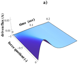
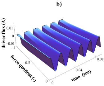
Figure 2: Time evolution of fluxes a)$J_{1}$ (driven) for DC–LCR circuit and b) $J_{2}$ (driver) for AC–LCR circuit versus force quotient $x^{\prime}$. There is a monotonous increasing behavior of each flux with $x^{\prime}$ in the direct and altern current cases. While in the temporal evolution of DC case there is a damped behavior but in AC case this behavior is oscillatory, due to frequency 60Hz of the sources and the respective values of the circuit elements are: $H_{1}=0.2\textrm{H},\,H_{2}=4\textrm{H},\,H_{3}=0.1\textrm{H},\,R_{1}=10\Omega,\,R_{2}=680\Omega,\,R_{3}=12\Omega,\,$, $C_{1}=3\mu F$, $C_{2}=500\mu F$ and $C_{3}=5\mu F$.

2.2.2 Altern Current LCR system

Now we can consider that LCR circuit is fed by alternanting voltage $X_{1}=X_{1}(t)=X_{01}\textrm{sin}\left(\omega t+\delta\right)$ and $X_{2}=X_{2}(t)=X_{02}\textrm{sin}\left(\omega t+\beta\right)$ applied at time $t=0$, besides $\omega$ is the angular frecuency and $\left(\delta,\,\beta\right)$ are the phase angles at time equal to zero, because $\textrm{sin}\left(\omega t+\varphi_{i}\right)$ can express the imaginary component of $\exp\left[i\left(\omega t+\varphi_{i}\right)\right]$. The system composed by (7) and (8) can be rewriten as:

$$i\omega X_{01}\exp\left(i\omega t\right)=\left[-\omega^{2}H_{T1}J_{01}+i\omega R_{T1}J_{01}+\left(\frac{1}{C_{1}}+\frac{1}{C_{2}}\right)J_{01}+\omega^{2}H_{2}J_{02}-i\omega R_{2}J_{02}-\frac{J_{02}}{C_{2}}\right]\exp\left(i\omega t\right),$$ (15)

and

$$i\omega X_{02}\exp\left(i\omega t\right)=\left[-\omega^{2}H_{T2}J_{02}+i\omega R_{T2}J_{02}+\left(\frac{1}{C_{2}}+\frac{1}{C_{3}}\right)J_{02}+\omega^{2}H_{2}J_{01}-i\omega R_{2}J_{01}-\frac{J_{01}}{C_{2}}\right]\exp\left(i\omega t\right),$$ (16)

where $\delta=\beta=0$, i.e, the voltage sources are not out of phase. If we divide both equations by $i\omega\exp\left(i\omega t\right)$, then we obtain a new equations system,

$$\left[\begin{array}[]{c}X_{01}\\ X_{02}\end{array}\right]=\left[\begin{array}[]{cc}i\omega H_{T1}+R_{T1}+\frac{1}{i\omega}\left(\frac{1}{C_{1}}+\frac{1}{C_{2}}\right)&-\left(i\omega H_{2}+R_{2}+\frac{1}{i\omega C_{2}}\right)\\ -\left(i\omega H_{2}+R_{2}+\frac{1}{i\omega C_{2}}\right)&i\omega H_{b2}+R_{T2}+\frac{1}{i\omega}\left(\frac{1}{C_{2}}+\frac{1}{C_{3}}\right)\end{array}\right]\left[\begin{array}[]{c}J_{01}\\ J_{02}\end{array}\right],$$ (17)

taking into account the circuit impedances: $Z_{12}=Z_{1}+Z_{2}=i\omega H_{b1}+R_{b1}+\frac{1}{i\omega}\left(\frac{1}{C_{1}}+\frac{1}{C_{2}}\right)$, $Z_{2}=i\omega H_{2}+R_{2}+\frac{1}{i\omega C_{2}}$ and $Z_{23}=Z_{2}+Z_{3}=i\omega H_{b2}+R_{b2}+\frac{1}{i\omega}\left(\frac{1}{C_{2}}+\frac{1}{C_{3}}\right)$, with $R_{b1}=R_{1}+R_{2}$ and $R_{b2}=R_{2}+R_{3}$ the sum of the resistances of each mesh. Thus, steady states appear in frecuency space because current and voltages are linearly related in AC circuits (Figure 2b).

Therefore, the previous system can be inverted as follows:

$$\left[\begin{array}[]{c}J_{01}\\ J_{02}\end{array}\right]=\left[\begin{array}[]{cc}\mid\frac{Z_{2}+Z_{3}}{\triangle}\mid\textrm{sen}\left(\omega t-\theta_{23}\right)&\mid\frac{Z_{2}}{\triangle}\mid\textrm{sen}\left(\omega t-\theta_{2}\right)\\ \mid\frac{Z_{2}}{\triangle}\mid\textrm{sen}\left(\omega t-\theta_{2}\right)&\mid\frac{Z_{1}+Z_{2}}{\triangle}\mid\textrm{sen}\left(\omega t-\theta_{12}\right)\end{array}\right]\left[\begin{array}[]{c}X_{10}\\ X_{20}\end{array}\right],$$ (18)

with $\triangle=\left(Z_{2}+Z_{3}\right)\left(Z_{1}+Z_{2}\right)-Z_{2}^{2}$, the determinant of (17) and

$$\theta_{23}=\arctan\left(\frac{\textrm{Im}\left[\frac{Z_{2}+Z_{3}}{\triangle}\right]}{\textrm{Re}\left[\frac{Z_{2}+Z_{3}}{\triangle}\right]}\right),\,\theta_{2}=\arctan\left(\frac{\textrm{Im}\left[\frac{Z_{2}}{\triangle}\right]}{\textrm{Re}\left[\frac{Z_{2}}{\triangle}\right]}\right)\,\textrm{and}\,\theta_{12}=\arctan\left(\frac{\textrm{Im}\left[\frac{Z_{1}+Z_{2}}{\triangle}\right]}{\textrm{Re}\left[\frac{Z_{1}+Z_{2}}{\triangle}\right]}\right).$$

From (18) we remark again the time dependence of the coefficients $L_{ij}$.

3 Energetic of the LCR–circuit

Now we take this linear isothermic–isobaric model of conversion process and build its characteristic functions in terms of $q(t)$ and $x(t)$ for determining the performance condition corresponding to the maximization of a certain objective function. Firstly, we take into account the temporal evolution of the above mentioned parameters. From (13) and (18), we study the behavior when the inductors are saturated, so the circuit turns purely dissipative. On the other hand, when the capacitors are saturated, there are no longer currents. The saturation time is related to the circuit characteristic time. For the study of the energetics of the converter we consider characteristic functions as the dissipation function, the power output and efficiency, as well as objective functions as the ecological function and the efficient power. These functions can be written in terms of parameters $\left[q(t),\,x(t)\right]$.

We have considered the conventional values of inductances, capacitances and resistances reported in literature of electric circuits [19]; in this case we take the following values: $H_{1}=0.2\textrm{H},\,H_{2}=4\textrm{H},\,H_{3}=0.1\textrm{H},\,R_{1}=10\Omega,\,R_{2}=680\Omega,\,R_{3}=12\Omega,\,$, $C_{1}=3\mu F$, $C_{2}=500\mu F$ and $C_{3}=5\mu F$.

3.1 Efficiency

We define the efficiency of the thermodynamic process as the ratio of useful energy output divided by energy input, which is in general supplied to the system. If we take the Caplan and Essig idea [13], efficiency can be obtained in terms of Onsager relations as follows:

$$\eta[L_{ij}(t)]=-\frac{TJ_{1}X_{1}}{TJ_{2}X_{2}}=-\frac{x(t)\left[x(t)+q(t)\right]}{q(t)x(t)+1}=-\frac{\left(x^{\prime}\right)^{2}L_{11}(t)+x^{\prime}L_{12}(t)}{x^{\prime}L_{12}(t)+L_{22}(t)}.$$ (19)

The graph (Figure 3a) of this function is a convex surface with only one maximum point. This point shows an exclusive relationship between the input and output fluxes which maximize the efficiency for some Onsager coefficients. On the other hand, the temporal behavior is monotonically increasing and tends to an asymptotic value. In the AC circuit, efficiency has a maximum for the same value of $x^{\prime}$, although it becomes a periodic function of time (not shown here).

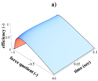
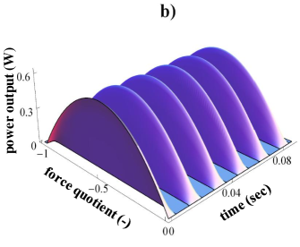
Figure 3: a) Efficiency for DC–LCR circuit and b) power output for AC–LCR circuit for $X_{2}^{2}$ fixed and $T=300\textrm{K}$ versus time and $x^{\prime}$.

3.2 Power output

For an isothermal process of two coupled fluxes this energetic function is given by [11, 20]

$$P[L_{ij}(t)]=-TJ_{1}X_{1}=-x(t)\left[x(t)+q(t)\right]TL_{22}(t)X_{2}^{2}=-\left[\left(x^{\prime}\right)^{2}L_{11}(t)+x^{\prime}L_{12}(t)\right]TX_{2}^{2}.$$ (20)

This equation corresponds to a convex surface with a maximum absolute value at $x^{\prime}$, where it is clearly shown that this maximum is maintained with the same value along Figure3b, i.e, the circuit has reached a steady state, because of the circuit’s characteristic time is less than the time corresponding to $60\,\textrm{Hz}$ . In the DC circuit (which is not shown here) this function reaches a maximum value at the same $x^{\prime}$. However, there is a damped oscillation in time corresponding to another aspect of the same phenomenon. This means, that the energetic compromise of the system is only due to the parameter $x^{\prime}$.

3.3 Dissipation function

The entropy production for a $(2\times 2)$ system of fluxes and forces in general is given by [13, 21],

$$\sigma=J_{1}X_{1}+J_{2}X_{2}$$ (21)

and as mentioned by several authors [13, 14], the dissipation function for isothermal systems is $\Phi=T\sigma$. By the substitution of (5) and (6) into (21) we obtain $\Phi$ in terms of the parameters $q(t)$, $x(t)$ and the coefficients $L_{ij}(t)$, namely

$$\Phi[L_{ij}(t)]=\left[x^{2}(t)+2x(t)q(t)+1\right]TL_{22}(t)X_{2}^{2}=\left[\left(x^{\prime}\right)^{2}L_{11}(t)+2x^{\prime}L_{12}(t)+L_{22}(t)\right]TX_{2}^{2}.$$ (22)

This function is a concave surface with a minimum value with respect to force quotient $x^{\prime}$ as well as the steady state too (see Figure 4a). In the AC case, the same value is obtained but it appears with a frequency of 60 times per second. This surface is not shown here.

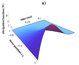
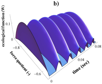
Figure 4: a) Dissipation function for DC–LCR circuit and b) ecological function AC–LCR circuit for $X_{2}^{2}$ fixed and $T=300\textrm{K}$ versus time and $x^{\prime}$. We observe that the evolution over time is determined by the dynamics of each system.

3.4 Ecological function

Defining the ecological function as an objetive function ($E=P-\Phi$) [22], by means of (22) and (20) we get

$$E[L_{ij}(t)]=-\left[2x^{2}(t)+3x(t)q(t)+1\right]TL_{22}(t)X_{2}^{2}=-\left[\left(x^{\prime}\right)^{2}L_{11}(t)+3x^{\prime}L_{12}(t)+L_{22}(t)\right]TX_{2}^{2}.$$ (23)

This equation also corresponds to a convex surface with only a maximum point at $x^{\prime}$. Now, we see in Figure 4b as well as for the similar direct current case (damped oscillation, which is not shown here), that a good compromise between power output and dissipated energy is modulated by the presence of transient elements and the oscillatory behavior over time is kept.

3.5 Efficient power output

Another objective function to treat is the efficient power, defined as the direct product between power output and efficiency [14, 18], using (20) and (19) we get:

$$P_{\eta}[L_{ij}(t)]=\frac{x^{2}(t)\left[x(t)+q(t)\right]^{2}TL_{22}(t)X_{2}^{2}}{q(t)x(t)+1}=\frac{\left[\left(x^{\prime}\right)^{2}L_{11}(t)+x^{\prime}L_{12}(t)\right]^{2}TX_{2}^{2}}{x^{\prime}L_{12}(t)+L_{22}(t)}.$$ (24)

In Figure 5 we observe that the surfaces for power output and efficiency have a maximum point. Then the efficient power presents a convex behavior with a maximum value too (see Figure 5). This regime will be analyzed in the next Section. Nevertheless, one can see the same behavior with respect to the parameter $x^{\prime}$, which is related to the exchange of energy, as the temporal behavior is governed by the nature of the sources.

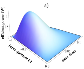
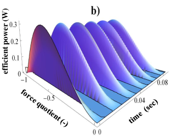
Figure 5: Efficient power for a) DC and b) AC LCR circuit for $X_{2}^{2}$ fixed and $T=300\textrm{K}$ versus time and $x^{\prime}$. Efficient power reaches a maximum value at an especific $x^{\prime}$, means, there is a unique fraction of $X_{1}$ due to the presence of $X_{2}$ in order to obtain a maximum efficient power regime.

From the values for inductances, capacitances and resistances set out at the begining of this section, we verify in Figures 3, 4, and 5 the well–know temporal behavior in circuit theory, furthermore those functions agree with the characteristic curves for steady states. The values of the circuit elements were taken in order to obtain a coupling between the circuit meshes.

Finally, when we take $C_{i}\rightarrow\infty$, that is, any sources or sinks of potential differences appear, we can recover the results for a LR circuit. While $H_{i}=0$, there are no source or sink of currents in the circuit, the LCR circuit becomes a CR circuit.

4 A performance mode of the LCR converter

From the figures in the previous section, we see that every characteristic function reaches maximum or minimal values, which are found by means of $\nicefrac{{dP_{\eta}(t)}}{{dx}}\mid_{x_{MEP}}=0$. In this case the force ratio value that maximizes the efficient power is given by

$$x_{MEP}(t)=-\frac{4+q^{2}(t)-\sqrt{16-16q^{2}(t)+q^{4}(t)}}{6q(t)}.$$ (25)

Replacing this force ratio value in each of the expressions for the characteristic functions, one can ensure that the converter operates in the maximum efficient power regime (MEP) [23], hence:

$$\eta_{MEP}(t)=-\frac{4\left(2+q^{2}(t)+\alpha(t)\right)}{3q^{2}(t)},$$ (26)

$$P_{MEP}(t)=\frac{\left(4+q^{2}(t)-\alpha(t)\right)\left(-4+5q^{2}(t)+\alpha(t)\right)}{36q^{2}(t)}TL_{22}(t)X_{2}^{2},$$ (27)

$$\Phi_{MEP}(t)=\frac{\left[-5+\left(-4+\alpha(t)\right)q^{4}(t)+\left(-2+\alpha(t)\right)5q^{2}(t)\right]}{18q^{2}(t)}TL_{22}(t)X_{2}^{2},$$ (28)

$$E_{MEP}(t)=\frac{\left[7q^{4}(t)+\left(26-7\alpha(t)\right)q^{2}(t)+8\left(-4+\alpha(t)\right)\right]}{18q^{2}(t)}TL_{22}(t)X_{2}^{2},$$ (29)

$$P_{\eta MPE}(t)=\frac{\left(4+q^{2}(t)-\alpha(t)\right)^{2}\left(-4+5q^{2}(t)+\alpha(t)\right)^{2}}{\left(-2+q^{2}(t)-\alpha(t)\right)216q^{4}(t)}TL_{22}(t)X_{2}^{2},$$ (30)

where $\alpha(t)=\sqrt{16-16q^{2}(t)+q^{4}(t)}$. In the graphs of Figures 6 and 7,

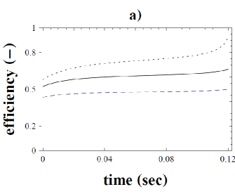
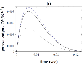
Figure 6: Normalized energetic functions (efficiency and power output) are evaluated in the regimes: OE $\left(x_{OE}=-\nicefrac{{q(t)}}{{1+\sqrt{1-q^{2}(t)}}}\right)$ (dotted line), MPO $\left(x_{MPO}=-\nicefrac{{q(t)}}{{2}}\right)$ (dashed line) and MEP (solid line) for $TX_{2}^{2}$ fixed versus time, for the DC case. Power output evaluated in each regimen reaches a maximum point at different time values.

we note that process variables of LCR–circuit evaluated in the regime of operation: maximum power output (MPO), optimum efficiency (OE) and MPE are in function of the circuit characteristic time. Moreover power output and dissipation function evaluated in each regime are governed by a damping behavior in the circuit. For that reason, the energy conversion process stops at some multiple of the circuit characteristic time. In Figure 6a we show that $\eta_{MPO}<\eta_{MEP}<\eta_{OE}$. This means that MPE regime can offer an attainable optimum compromise between energy output and energy input, even for non–stationary energy converters. Otherwise, in Figs. 6b and 7

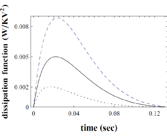
Figure 7: Normalized dissipation function is evaluated in the regime: oe $\left(x_{OE}=-\nicefrac{{q(t)}}{{1+\sqrt{1-q^{2}(t)}}}\right)$(dotted line), MPO $\left(x_{MPO}=-\nicefrac{{q(t)}}{{2}}\right)$ (dashed line) and MEP (solid line) for $TX_{2}^{2}$ fixed versus time, for the DC case. We see that dissipation function evaluated in each regimen reaches a maximum point at different time values.

the MPE regime displays a good coupling between the driver flux and the driven flux, in order to obtain the power output. In the case of AC, all the functions keep the same shape but time evolution is totally oscillatory.

5 Conclusions.

In this work we have studied an energy converter with non–steady processes. This is due to transient elements in the converter (LCR–circuit). Therefore, the energy conversion depends on time. Nevertheless, there is a time longer than the characteristic time of the circuit for which this converter reaches a steady state. In the first place, linearization of the circuit’s dynamic equations (Kirchhoff equations) allow us to construct generalized flows and forces. The Onsager symmetry relation between cross coefficients ($L_{12}(t)=L_{21}(t)$) are found at any time. The evolution of the converter is governed by the behavior of the coupling coefficients. When the inductors are saturated, $q$ asymptotically reaches a constant value in time and the energy exchange is fixed. On the other hand when capacitors are saturated, $q$ decays until the energy exchange stops. Efficient power as a performance mode of an energy converter could be a suitable regime of operation, because efficiency evaluated in MPE regime is bigger than MPO regime, with a small decrement in power output and a large decrement in dissipated energy.

From these results we will be able to study other converters of the same nature with an appropriate energetic performance. The damped behavior of the circuit is due to the values taken for the passive and transients elements, because we must ensure that this converter operates in a coupled regime.

References

- [1] E. Hernández–Lemus, H. Tovar and C. Mejía, Non–equilibrium thermodynamics analysis of transcriptional regulation kinetics, J. Non–Equilib. Thermodyn., 39 (2014), 205–218.
- [2] I. Santamaría–Holek, A. Pérez–Madrid and J. M. Rubi, Local Quasi–equilibrium Description of Multsacle Systems, J. Non–Equilib. Thermodyn., 41 (2016), 123–130.
- [3] J. L. Garden, H. Guillou, J. Richard and L. Wondraczek, Non–equilibrium configurational Progogine-Defay ratio, J. Non–Equilib. Thermodyn., 37 (2012), 143–147.
- [4] J. Gonzalez–Ayala, R. Cordero and F. Angulo–Brown, Is the nature of the universe a thermodynamic necessity?, EPL; 113 (2016) 40006.
- [5] P. T. Landsberg and A. De Vos, The Stefan–Boltzmann constant in n-dimensional space, J. Phys. A: Math. Gen., 22 (1989), 1073–1084.
- [6] G. Ares de Parga, B. López–Carrera and F. Angulo–Brown, A proposal for relativistic transformation in thermodynamics, J. Phys. A: Math. Gen., 38 (2005), 2821–2834.
- [7] J. Gonzalez–Ayala, L. A. Arias–Hernández and F. Angulo–Brown, Conection between maximum–work and maximum–power thermal cycles, Phys Rev E 88 (2013), 052142.
- [8] Ramandeep S. Johal, Efficiency at optimal work from finite source and sink: A probabilistic perspective, J. Non–Equilib. Thermodyn., 40 (2015), 1–12.
- [9] I. Prigogine, Thermodynamics of Irreversible Processes, Ed. J. Wiley–Interscience, NY third edition, 1967.
- [10] L. A. Arias-Hernandez, F. Angulo-Brown and R. T. Paez-Hernandez, First-order irreversible thermodynamics approach to a simple energy converter, Phys Rev E 77 (2008), 011123.
- [11] H. T. Odum and R. C. Pinkerton, Time’s speed regulator, Am. Sci. 43, (1955), 331–343.
- [12] K. H. Hoffmann, J. M. Burzler and S. Schubert, Endoreversible Thermodynamics, J. Non–Equilib. Thermodyn. 22 (1997), 311–355.
- [13] S. R. Caplan and A. Essig, Bioenergetics and Linear Nonequilibrium Thermodynamics: the Steady State, 1st ed., Cambridge, MA: Ed. Harvad University Press, 1983.
- [14] J. W. Stucki, The optimal efficiency and the economics degrees of coupling of oxidative phosphorylation, Eur. J. Biochem. 109 (1980), 269–283.
- [15] M. Tribus, Thermostatics and Thermodynamics, 1st ed., D. Van Nostrand Co., Princeton 1961.
- [16] L. Onsager, Reciprocal relations in irreversible processes I, Phys. Rev., 37 (1931), 405–426.
- [17] F. Angulo–Brown, L.A. Arias–Hernández and M. Santillán, On some connections between first order irreversible thermodynamics and finite-time thermodynamics, Rev. Mex. Fis, 48S (2002), 182–192.
- [18] T. Yilmaz, A new performance criterion for heat engines, J. Energy Inst., 79 (2006), 38–41.
- [19] J. A. Edminister, Electric Circuits, 1st ed., Mc. Graw-Hill, 1965.
- [20] M. Santillan, L. A. Arias–Hernandez and F. Angulo–Brown, Some optimization criteria for biological systems in linear irreversible thermodynamics, Il Nuovo Cimento Soc. Ital. Fis. D, 17 (1999), 87–90.
- [21] S. R. De Groot and P. Mazur, Non–Equilibrium Thermodynamics, 1st ed., North-Holland Publ. Co., Amsterdam, 1962.
- [22] F. Angulo–Brown, An ecological optimization criterion for finite-time heat engines, J. Appl. Phys., 69 (1991), 7465–7469.
- [23] G. Valencia–Ortega, Algunos convertidores de energía con flujos y fuerzas no estacionarios: circuitos RC, RL y RLC, Master Thesis, Instituto Politécnico Nacional, México, 2015 (in Spanish).