The Numerical Approximation of Nonlinear Functionals and Functional Differential Equations

Abstract

The fundamental importance of functional differential equations has been recognized in many areas of mathematical physics, such as fluid dynamics (Hopf characteristic functional equation), quantum field theory (Schwinger-Dyson equations) and statistical physics (equations for generating functionals and effective Fokker-Planck equations). However, no effective numerical method has yet been developed to compute their solution. The purpose of this report is to fill this gap, and provide a new perspective on the problem of numerical approximation of nonlinear functionals and functional differential equations.

1 Introduction

In this report we address a rather neglected but very important research area in computational mathematics, namely the numerical approximation of nonlinear functionals and functional differential equations (FDEs). FDEs are arise naturally in many different areas of mathematical physics. For example, in the context of fluid dynamics, the Hopf equation [89]

$$\frac{\partial\Phi([\bm{\theta}],t)}{\partial t}=\sum_{k=1}^{3}\int_{V}\theta_{k}(\bm{x})\left(i\sum_{j=1}^{3}\frac{\partial}{\partial x_{j}}\frac{\delta^{2}\Phi([\bm{\theta}],t)}{\delta\theta_{k}(\bm{x})\delta\theta_{j}(\bm{x})}+\nu\nabla^{2}\frac{\delta\Phi([\bm{\theta}],t)}{\delta\theta_{k}(\bm{x})}\right)d\bm{x},$$ (1)

was deemed by Monin and Yaglom ([145], Ch. 10) to be “the most compact formulation of the general turbulence problem”, which is the problem of determining the statistical properties of the velocity and the pressure fields of Navier-Stokes equations given statistical information on the initial state. In equation (1) $V\subset\mathbb{R}^{3}$ is a periodic box, $\bm{\theta}(\bm{x})=(\theta_{1}(\bm{x}),\theta_{2}(\bm{x}),\theta_{3}(\bm{x}))$ is a vector-valued test function in a suitable divergence-free space, and $\Phi$ is a nonlinear complex-valued functional known as Hopf functional [89]. Remarkably, with such functional available it is possible to compute any statistical property of the velocity field that solves the Navier-Stokes equations (see [145]). This is of great conceptual importance: the solution to one single linear functional differential equation can describe all statistical features of turbulence and there is no need to refer back to the Navier-Stokes equations. From a mathematical viewpoint the Hopf functional is basically a time-dependent nonlinear operator in the space of test functions $D(\Phi)$ (domain of the operator $\Phi$) with range in the complex plane (see Figure 1).

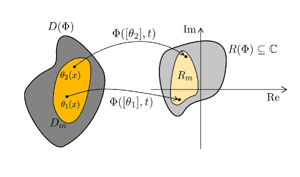
Figure 1: Sketch of the mapping at the basis of the Hopf functional. The domain of the functional $\Phi$, denoted as $D(\Phi)$ is a suitable of space of functions while the range of $\Phi$, denoted as $R(\Phi)$, is a subset of the complex plane $\mathbb{C}$. The approximation space $D_{m}$ is a subset of $D(\Phi)$, which is mapped into $R_{m}$.

The operator can be formally defined as a functional integral

$$\Phi([\bm{\theta}],t)=\int_{\Omega}\exp\left[i\int_{V}\bm{u}(\bm{x},t;\omega)\cdot\bm{\theta}(\bm{x})d\bm{x}\right]P([\bm{u}_{0}])\mathcal{D}[\bm{u}_{0}]$$ (2)

where $\bm{u}(\bm{x},t;\omega)$ is a stochastic solution to the Navier-Stokes equations and $P([\bm{u}_{0}])$ is the probability functional of the random initial state (assuming it exists). Thus, computing the solution to the Hopf equation (1) is equivalent to compute a (complex-valued) time-dependent nonlinear operator $\Phi$ from an equation that involves classical partial derivatives with respect to space and time variables as well as derivatives with respect to functions, i.e., functional derivatives $\delta/\delta\theta_{j}(\bm{x})$ [220, 154].

Another example of functional differential equation is the Schwinger-Dyson equation of quantum field theory [49, 252]. Such equation describes the exact dynamics of the Green functions of a general field theory, and it allows us to propagate field interactions, either in a perturbation setting [165] (weak coupling regime) or in a strong coupling regime [212]. The Schwinger-Dyson formalism is also useful in computing the statistical properties of stochastic dynamical systems. For example, consider Langevin equation

$$\frac{d\bm{\psi}(t)}{dt}=\bm{G}(\bm{\psi}(t),t)+\bm{f}(t;\omega),$$ (3)

where $\bm{f}(t;\omega)$ is random noise. Define the generating functional [174, 96]

$$Z([\bm{\xi},\bm{\eta}])=Z_{0}\int\mathcal{D}[\bm{\psi}]\mathcal{D}[\bm{\beta}]A([\bm{\psi},\bm{\beta}])\exp\left[\int_{0}^{t}d\tau\left(\bm{\xi}(\tau)\cdot\bm{\psi}(\tau)+\bm{\eta}(\tau)\cdot\bm{\beta}(\tau)\right)\right],$$ (4)

where $Z_{0}$ is a normalization constant and

$$A([\bm{\psi},\bm{\beta}])=C([\bm{\beta}])\exp\left[-\frac{1}{2}\int_{0}^{t}d\tau\nabla\cdot\bm{G}(\bm{\psi}(\tau),\tau)-i\int_{0}^{t}d\tau\bm{\beta}(\tau)\cdot\left(\frac{d\bm{\psi}(\tau)}{dt}-\bm{G}(\bm{\psi}(\tau),\tau)\right)\right].$$ (5)

The functional $C([\bm{\beta}])$ in (5) denotes the (known) characteristic functional of the external random noise $\bm{f}(t;\omega)$. Clearly, if we have available the stochastic solution to (3), then we can construct the functional $Z([\bm{\xi},\bm{\eta}])$ and compute all statistical properties we are interested in. On the other hand, it is straightforward to show that $Z([\bm{\xi},\bm{\eta}])$ satisfies the following system of linear FDEs (Schwinger-Dyson equations)

$$\frac{1}{i}\frac{\partial}{\partial\tau}\frac{\delta Z}{\delta\xi_{k}(\tau)} =\eta_{k}(\tau)Z+G_{k}\left(\frac{1}{i}\frac{\delta}{\delta\bm{\xi}(\tau)},\tau\right)Z-iD_{k}\left(\left[\frac{1}{i}\frac{\delta}{\delta\bm{\eta}(\tau)}\right],\tau\right)Z,$$ (8)

$$\frac{1}{i}\frac{\partial}{\partial\tau}\frac{\delta Z}{\delta\eta_{k}(\tau)} =-\xi_{k}(\tau)Z+i\sum_{j=1}^{n}\frac{\delta}{\delta\eta_{j}(\tau^{+})}\frac{\partial G_{k}}{\partial\psi_{j}}\left(\frac{1}{i}\frac{\delta}{\delta\bm{\xi}(\tau)},\tau\right)Z,$$ (9)

where

$$D_{i}([\bm{\beta}],\tau)=\frac{\delta C([\bm{\beta}])}{\delta\beta_{i}(\tau)}.$$ (10)

The solution to the Schwinger-Dyson equations (8)-(9) is a nonlinear functional (i.e., a nonlinear operator) $Z([\bm{\xi},\bm{\eta}])$ which allows us to compute all statistical properties of the system without any knowledge of the stochastic process $\bm{\psi}(t;\omega)$ defined implicitly by the stochastic ODE (3). By generalizing (4), it is possible to derive a functional formalism for any classical field theory or stochastic system. This yields, in particular, Schwinger-Dyson-type equations for generating functionals associated with the solution to stochastic partial differential equations (SPDEs). If the SPDE admits an action functional, then the construction of the generating functional as well as the derivation of the corresponding Schwinger-Dyson equation are rather straightforward (see [96, 5, 109]).

The usage of functional differential equations grew very rapidly during the sixties, when it became clear that techniques developed for quantum field theory by Dyson, Feynman, and Schwinger could be applied, at least formally, to other branches of mathematical physics. The seminal work of Martin, Siggia, and Rose [136] became a landmark on this subject, since it revealed the possibility of applying (at least formally) quantum field theoretic methods, such as functional integrals and diagrammatic expansions [174, 96, 173, 97], to classical physics. Relevant applications of these techniques can be found in non-equilibrium statistical mechanics [96, 174, 173, 97, 58, 117, 217, 218], stochastic dynamics [87, 228, 112], and turbulence theory [67, 139, 59, 29, 73, 46, 3, 124, 144, 145, 193, 194, 197, 148, 90].

An open question that has persisted over the years is: How do we compute the solution to a functional differential equation? From the fifties to the eighties, researchers were of course investigating analytical methods, e.g., based on functional power series [193, 194, 231, 155], functional integrals [109, 127, 177, 51], transforms with respect to appropriate measures ([145], p. 802), and diagrammatic expansions. More recently, Waclawczyc and Oberlack [162, 232] proposed a Lie group analysis and applied it to the Hopf-Burgers equation, which represents a step forward toward developing new analytical solution methods. Specifically, invariant solutions of the Hopf-Burgers equation were found based on the analysis of the infinitesimal generator of suitable symmetry transformations. From a numerical viewpoint, recent advances in computational mathematics – in particular in numerical tensor methods [78] – open the possibility to solve functional differential equations on a computer. In this report, we will present state-of-the-art mathematical techniques and numerical algorithms to represent nonlinear functionals and compute the numerical solution to functional differential equations.

If FDEs are so important, why do they not have a prominent role in computational mathematics? There are several possible answers to this question. First of all, FDEs are infinite-dimensional equations, in the sense that they are, in principle, equivalent to an infinite-dimensional system of PDEs, or PDEs in an infinite number of variables. This may have understandably discouraged researchers in numerical analysis to even attempt a numerical discretization. Most schemes proposed so far are based on truncations of infinite hierarchies of PDEs obtained, e.g, from functional power series expansions [193, 194, 197, 196, 145, 2, 67], or Lundgren-Monin-Novikov hierarchies [233, 66, 130, 90, 198]. Other approaches are based on a direct discretization of the functional integral [109, 51, 177, 117] that defines the field theory (e.g. $Z$ in equation (4)), and its evaluation using Monte Carlo methods, or source Galerkin methods [120, 119]. Dealing with systems of infinitely many PDEs or very high-dimensional PDEs can indeed be discouraging, but nowadays it is quite common, for example when discretizing stochastic systems driven by colored random noise or stochastic partial differential equations (SPDEs) [250, 242, 234, 244, 230]. Another reason why FDEs have not yet been numerically studied extensively may be due to a lack of awareness of their existence within the computational mathematics community. Also, there is no universal agreement across scientific disciplines as to even the basic definition of an FDE. For example, most applied mathematics literature refers to FDEs as ordinary differential equations with memory or delay terms [241, 7, 80]. In the pure mathematics community, functional equations have been studied in the context of approximate homeomorphisms (the Ulam stability problem) [186, 187], or more generally within problems where the unknown is a function, e.g., Cauchy or d’Alambert functional equations [201]. The physics literature, on the other hand, clearly identifies FDEs as those equations whose unknown is a functional (i.e., a nonlinear operator) and that involve partial derivatives with respect to independent variables (e.g., space and time), as well as derivatives with respect to functions (functional derivatives). These kinds of equations are usually far more challenging than the functional equations studied by the pure mathematics community, and indeed there are very few general theorems on the existence and the uniqueness of their solution [80, 63].

In this report we take the physicist viewpoint and consider linear functional differential equations in the form

$$\frac{\partial F([\bm{\theta}],t)}{\partial t}=L([\bm{\theta}],t)F([\bm{\theta}],t)+H([\bm{\theta}θ],t),\qquad F([\bm{\theta}],0)=F_{0}([\bm{\theta}]),$$ (11)

where $F([\bm{\theta}],t)$ is a real or complex-valued functional (time-dependent nonlinear operator in a space of functions), $F_{0}([\bm{\theta}])$ is a given initial condition, $L([\bm{\theta}],t)$ is a linear operator in the space of nonlinear functionals, and $H([\bm{\theta}],t)$ is a known forcing functional. The linear operator $L([\bm{\theta}],t)$ usually involves functional derivatives with respect to $\bm{\theta}(\bm{x})$ as well as partial derivatives with respect to independent variables, e.g, space and time coordinates. For example, $L([\bm{\theta}],t)$ could be the linear operator defining the right hand side of equation (1). We emphasize that the class of equations in the form (11) is very broad as it encompasses FDEs describing many physical systems, including statistical properties of nonlinear SODEs and SPDEs (e.g., Hopf characteristic functional equations [89, 148, 145, 112] or equations for probability density functionals [73, 15, 46]), functional equations arising in control theory [14], generalized principles of least actions [225], and functional equations of quantum field theory [252, 95, 174, 97, 96, 117].

To the best of our knowledge, no effective numerical methods have yet been developed to compute the solution to linear functional differential equations in the form (11), and little has been done for functional differential equations in general, despite their fundamental importance in many areas of mathematical physics. The purpose of this report is to fill this gap and present state-of-the-art mathematical techniques, including new classes of numerical algorithms, to approximate nonlinear functionals and the numerical solution to functional differential equations in the form (11) This report is organized in two parts:

1. Approximation of Nonlinear Functionals A nonlinear functional is a particular type of nonlinear operator from a space of functions into a vector space, e.g., $\mathbb{R}$ or $\mathbb{C}$. Therefore, the process of approximating a nonlinear functional is basically the same as approximating a nonlinear operator [92, 216, 14]. In this report we will present various techniques for nonlinear functional approximation, ranging from polynomial functional series expansions, to expansions based on stochastic processes, and functional tensor methods. Within the context of polynomial functional series expansions we will discuss in particular Lagrange interpolation in Hilbert and Banach spaces [134, 183, 181, 17, 4, 28], where the interpolation “nodes” are functions in a suitable function space. We will also discuss series expansions based on functional tensor methods [78]. This class of methods relies on recent developments on multivariate function approximation such as canonical polyadic (CP) [188, 18, 113] and hierarchical Tucker (HT) [8, 77] series expansions.

2. Approximation of Functional Differential Equations A functional differential equation is an equation whose solution is a nonlinear functional, i.e., a nonlinear operator. The equation usually involves functional derivatives of such functional and partial derivatives and integrals with respect to independent variables. The goal of approximation theory for functional differential equations is therefore to determine an approximation of such nonlinear functional, e.g., its time evolution given an initial state. In this report we will discuss new classes of methods that extend classical Galerkin, least-squares, and collocation techniques to functional differential equations. These methods are based on suitable representations of the solution functional, e.g., in terms of polynomial functionals or functional tensor networks.

This paper is organized as follows: In Section 2 we briefly review what nonlinear functionals, functional derivatives and provide useful examples of nonlinear functionals in physics. In Section 3 we address the approximation of nonlinear functionals and functional derivatives. In particular, we discuss Lagrange interpolation in spaces of infinite dimensions (function spaces), series expansions in terms of polynomial functionals, and functional tensor methods such as canonical polyadic and hierarchical Tucker expansions. In Section 4 we discuss functional differential equations. We begin by presenting several examples of FDEs and show how they arise in the context of well-known physical theories. In Section 5 we address the problem of computing the numerical solution to an FDE. Specifically, we introduce infinite-dimensional extensions of least squares, Galerkin, and collocation methods. Finally, in Section 6 and Section 7 we present numerical results on nonlinear functional approximation and also compute the numerical solution to a prototype functional advection-reaction problem.

2 Nonlinear Functionals

Let $X$ be a Banach space of functions. A nonlinear functional on $X$ is a nonlinear operator $F$ that takes in an element $\theta$ of $X$ (i.e., a function), and returns a real or a complex number. The functional $F$ usually does not operate on the entire linear space $X$ but rather on a subset set of$X$, which we denote as $D(F)\subseteq X$ (domain of the functional). Let us first provide simple examples of nonlinear functionals.

Example 1: Consider

$$F([\theta])=\int_{0}^{1}x^{3}e^{-\theta(x)}dx,\qquad\theta\in D(F)=C^{(0)}([0,1]),$$ (12)

where $C^{(0)}([0,1])$ is the space of continuous functions in $[0,1]$.

Example 2 (homogeneous polynomial functional of order $n$): Consider

$$P_{n}([\theta])=\underbrace{\int_{0}^{1}\cdots\int_{0}^{1}}_{\textrm{$n$ times}}K_{n}(x_{1},...,x_{n})\theta(x_{1})\cdots\theta(x_{n})dx_{1}\cdots dx_{n},$$ (13)

where $K_{n}$ are given kernel functions.

Example 3 (Ginzburg-Landau energy functional): The Ginzburg-Landau theory describes describes phase transitions and critical phenomena in a great variety of statistical systems ranging from magnetic systems, to diluted polymers and superconductors [110, 5]. At the basis of the theory is the energy functional

$$E([\phi])=\int_{\mathbb{R}^{3}}\left[\frac{1}{2}\left(\left|\nabla\phi(\bm{x})\right|^{2}+m^{2}\phi^{2}(\bm{x})\right)+\frac{\lambda}{4!}\phi^{4}(\bm{x})\right]d\bm{x}$$ (14)

where $m$ is the “mass” of the field $\phi$ and $\lambda$ is a coupling constant. In this case, the domain of the functional $E$ can be chosen as $D(E)=C^{(2)}(\mathbb{R}^{3})$.

Example 4 (Hopf characteristic functional of a Gaussian random field): Consider a scalar Gaussian random field $u(\bm{x};\omega)$ defined on a domain $V\subseteq\mathbb{R}^{3}$ it can be shown (see, e.g., [112]) that the Hopf characteristic functional of such random field is

$$\Phi([\theta])=\exp\left[i\int_{V}\mu(\bm{x})\theta(\bm{x})d\bm{x}-\frac{1}{2}\int_{V}\int_{V}C(\bm{x},\bm{y})\theta(\bm{x})\theta(\bm{y})d\bm{x}d\bm{y}\right],$$ (15)

where $\mu(\bm{x})$ and $C(\bm{x},\bm{y})$ denote, respectively, the mean and the covariance function of the field $u(\bm{x};\omega)$.

Analysis of nonlinear functionals in Banach spaces is a well-developed subject [220, 154, 203]. In particular, the classical definition of continuity and differentiability at a point that holds for real-valued functions can extended in a more or less straightforward way to nonlinear functionals. For instance, we say that a functional $F([\theta])$ is continuous at a point $\theta(x)\in D(F)$ if for any sequence of functions $\{\theta_{1}(x),\theta_{2}(x),...\}$ in $D(F)$) converging to $\theta$ we have that the sequence $\{F([\theta_{n}])\}$ converges to $\{F([\theta])\}$, i.e.,

$$\lim_{n\rightarrow\infty}\left|\theta_{n}(x)-\theta(x)\right|\rightarrow 0\quad\Rightarrow\quad\lim_{n\rightarrow\infty}\left|F([\theta_{n}])-F([\theta])\right|\rightarrow 0.$$ (16)

The functionals we discussed in Examples 1-4 are all continuous. From the continuity definition (16) it follows, in particular, that if $F([\theta])$ is continuous on a compact function space $D(F)$ then $F$ is bounded.

Example 4: Another example of a continuous functional in $D(F)=C^{(\infty)}([-1,1])$ is

$$F([\theta])=\theta(0)^{2}+\int_{-1}^{1}\sin(\theta(x))dx.$$ (17)

In fact, consider any sequence of functions $\{\theta_{n}\}$ in $D(F)$. Also choose an integrable function $g(x)$ such that $\left|\theta_{n}(x)\right|\leq g(x)$ for all $n\in\mathbb{N}$. In these conditions, the Lebesgue dominated convergence theorem applies and we have

$$\lim_{n\rightarrow\infty}\int_{-1}^{1}\sin(\theta_{n}(x))dx=\int_{-1}^{1}\sin(\theta(x))dx,$$ (18)

i.e.,

$$\theta_{n}\begin{subarray}{c}\rightarrow\end{subarray}\theta\,\Rightarrow\,F([\theta_{n}])\rightarrow F([\theta]).$$ (19)

2.1 Functional Derivatives

Consider a real or a complex valued functional $F$ defined on the function space $D(F)$ (domain of the functional). For simplicity, let us assume that $D(F)$ is a space of real valued functions $\theta(x)$ on the real line. We say that the functional $F$ is differentiable at $\theta(x)$ if the limit

$$\lim_{\epsilon\rightarrow 0}\frac{F([\theta(x)+\epsilon\eta(x)])-F([\theta(x)])}{\epsilon}$$ (20)

exists and it is finite. The quantity (20) is known as Gâteaux differential of $F$ in the direction of $\eta(x)$ (see, e.g., [220, 203]). Under rather general assumptions such derivative can be represented as a linear operator [154, 220, 225] acting on $\eta(x)$. For small $\epsilon$ we have

$$F([\theta(x)+\epsilon\eta(x)])=F([\theta(x)])+\epsilon L([\theta(x)])\eta(x)+R_{1}([\epsilon\eta(x);\theta(x)]),$$ (21)

In this series $L([\theta(x)])$ is a linear operator that sends the function $\eta(x)$ to a real or a complex number, while $R_{1}$ represents a reminder term. It is clear that $L([\theta(x)])$ involves integration with respect to $x$, since $L([\theta])\eta(x)$ is a real or complex number. Thus, we look for a representation of $L([\theta])\eta(x)$ in the form

$$L([\theta(x)])\eta(x)=\int\frac{\delta F([\theta])}{\delta\theta(x)}\eta(x)dx,$$ (22)

where the kernel function $\delta F([\theta])/\delta\theta(x)$ is a functional of $\theta$ and a function of $x$. At this point it is convenient to establish a parallel between functionals and functions in $m$ variables. Recall that the differential of a scalar field $f(a_{1},..,a_{m})$ in the direction $\widehat{n}=(n_{1},...,n_{m})$ is the scalar product of the gradient $\nabla f$ and $\widehat{n}$, i.e.,

$$df_{\widehat{n}}=\nabla f\cdot\widehat{n}.$$ (23)

By analogy, $\delta F([\theta])/\delta\theta(x)$ in equation (22) can be considered as an infinite-dimensional gradient, known as first-order functional derivative of $F$ with respect to $\theta(x)$.

The next question is: how do we compute such functional derivative? A possible way is to use the definition (20) and a compactly supported class of test functions, e.g., functions that are nonzero only in a small neighbor $\mathcal{I}_{x}(r)$ of radius $r$ centered at $x$. Such functions could be compactly supported elements of a Dirac delta sequence (see Figure 2), or even a delta function itself. This allows us to write

$$\frac{\delta F([\theta(x)])}{\delta\theta(x)}=\lim_{\epsilon,r\rightarrow 0}\frac{F([\theta(x)+\epsilon\alpha(x)])-F([\theta(x)])}{\displaystyle\epsilon\int_{\mathcal{I}_{x}(r)}\alpha(y)dy}$$ (24)

In particular, if we set $\alpha(y)=\delta(x-y)$ then the denominator in (24) simply reduces to $\epsilon$, yielding the formula

$$\frac{\delta F([\theta])}{\delta\theta(x)}= \lim_{\epsilon\rightarrow 0}\frac{F([\theta(y)+\epsilon\delta(x-y)])-F([\theta(y)])}{\epsilon}.$$ (25)

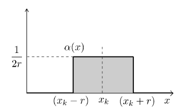
Figure 2: A possible function for the calculation of the kernel (24) at $x_{k}$. If we set $\mathcal{I}_{x_{k}}(r)=\{x\in\mathbb{R}:|x-x_{k}|\leq r\}$, then we have $\displaystyle\int_{\mathcal{I}_{x_{k}}(r)}\alpha(x)dx=1$, independently on $r$.

Functional derivatives of higher order can be defined in a similar manner. For example, the second order functional derivative of $F$ is

$$\frac{\delta^{2}F([\theta])}{\delta\theta(x)\delta\theta(y)}=\frac{d}{d\epsilon}\left[\frac{\delta F([\theta(z)+\epsilon\delta(z-y)])}{\delta\theta(x)}\right]_{\epsilon=0}.$$ (26)

Note that (26) is a function and $x$ and $y$ and a functional of $\theta(x)$.

Example 1: The first-order functional derivative of the nonlinear functional (12) can be obtained as follows. We first compute the Gâteaux differential

$$\frac{d}{d\epsilon}\left.F([\theta+\epsilon\eta])\right|_{\epsilon=0}= -\int_{0}^{1}x^{3}e^{-\theta(x)}\eta(x)dx$$

$$= \int_{0}^{1}\frac{\delta F([\theta])}{\delta\theta(x)}\eta(x)dx.$$ (27)

Therefore,

$$\frac{\delta F([\theta])}{\delta\theta(x)}=-x^{3}e^{-\theta(x)}.$$ (28)

Note that the functional derivative is a function of $x$ and a (local) functional of $\theta(x)$.

Example 2 (Functional Derivatives of the Hopf Functional): Consider the Hopf characteristic functional of a random function $u(x;\omega)$ defined in $[0,1]$

$$\Phi([\theta])=\left<\exp\left[i\int_{0}^{1}u(x;\omega)\theta(x)dx\right]\right>.$$ (29)

The average operator $\left<\cdot\right>$ here denotes a functional integral over the probability functional of $u(x,\omega)$. The Gâteaux differential of $\Phi([\theta])$ along $\eta$ is

$$\left.\frac{d}{d\epsilon}\Phi([\theta(x)+\epsilon\eta(x)])\right|_{\epsilon=0}= i\left<\exp\left[i\int_{0}^{1}u(x;\omega)\theta(x)dx\right]\int_{0}^{1}u(x;\omega)\eta(x)dx\right>$$

$$= \int_{0}^{1}i\left<\exp\left[i\int_{0}^{1}u(x;\omega)\theta(x)dx\right]u(x;\omega)\right>\eta(x)dx$$

$$= \int_{0}^{1}\frac{\delta\Phi([\theta])}{\delta\theta(x)}\eta(x)dx.$$ (30)

This implies that

$$\frac{\delta\Phi([\theta])}{\delta\theta(x)}=i\left<u(x;\omega)\exp\left[i\int_{a}^{b}u(x;\omega)\theta(x)dx\right]\right>$$ (31)

is the first-order functional derivative of $\Phi([\theta])$ at $\theta(x)$. Note that (31) is itself a functional of $\theta(x)$, which depends also on $x$. As a result, $\delta\Phi([\theta])/\delta\theta(x)$ has two types of derivatives: an ordinary one with respect to $x$, and a functional one with respect to $\theta(x)$. The latter is the the second-order functional derivative of $\Phi([\theta(x)])$. A simple calculation shows that

$$\frac{\delta^{2}\Phi([\theta])}{\delta\theta(x)\delta\theta(y)}=i^{2}\left<u(y;\omega)u(x;\omega)\exp\left[i\int_{a}^{b}u(x;\omega)\theta(x)dx\right]\right>.$$ (32)

Proceeding similarly, we can obtain the expression of higher-order functional derivatives. For instance, the third-order one is explicitly given as

$$\frac{\delta^{3}\Phi([\theta])}{\delta\theta(x)\delta\theta(y)\delta\theta(z)}=i^{3}\left<\exp\left[i\int_{a}^{b}u(x;\omega)\theta(x)dx\right]u(y;\omega)u(x;\omega)u(z;\omega)\right>.$$ (33)

Now, suppose we have available $\delta\Phi([\theta])/\delta\theta(x)$. Based on the definition (31), we see that

$$\left<u(x;\omega)\right>=\frac{1}{i}\frac{\delta\Phi([0])}{\delta\theta(x)}.$$ (34)

Similarly, higher order moments and cumulants of the random function $u(x;\omega)$ can be obtained by computing higher order functional derivatives of $\Phi([\theta(x)])$ and $\ln\Phi([\theta(x)])$, respectively, and evaluating them at $\theta(x)=0$. In particular, the second- and third-order correlation functions are, respectively

$$\left<u(x;\omega)u(y;\omega)\right>=\frac{1}{i^{2}}\frac{\delta^{2}\Phi([0])}{\delta\theta(x)\delta\theta(y)},\quad\left<u(x;\omega)u(y;\omega)u(z;\omega)\right>=\frac{1}{i^{3}}\frac{\delta^{3}\Phi([0])}{\delta\theta(x)\delta\theta(y)\delta\theta(z)}.$$ (35)

Example 3: The Gateaux differential of the nonlinear functional (17) in the direction $\eta(x)$ is

$$\left.\frac{d}{d\epsilon}F([\theta+\epsilon\eta])\right|_{\epsilon=0}= \frac{d}{d\epsilon}\left(\theta(0)+\epsilon\eta(0)+\int_{-1}^{1}\sin(\theta(x)+\epsilon\eta(x))dx\right)_{\epsilon=0}$$

$$=\int_{-1}^{1}\left(\delta(x)+\cos(\theta(x))\right)\eta(x)dx$$ (36)

Therefore the first-order functional derivative is

$$\frac{\delta F([\theta])}{\delta\theta(x)}=\delta(x)+\cos(\theta(x)),$$ (37)

where $\delta(x)$ at the right hand side is the Dirac delta function [98].

Regularity of Functional Derivatives

The last example clearly shows that functional derivatives of nonlinear functionals can easily be distributions [98], e.g., Dirac delta functions. For example, let $h\in C^{(\infty)}(\mathbb{R})$. Then any functional in the form $F([\theta])=h((\theta,\theta))$, where $(,)$ is an inner product in $C^{(\infty)}(\mathbb{R})$, has a singular second-order functional derivative. In fact,

$$\frac{\delta F([\theta])}{\delta\theta(x)}=2\left.\frac{\partial h}{\partial a}\right|_{a={(\theta,\theta)}}\theta(x)$$ (38)

$$\frac{\delta^{2}F([\theta])}{\delta\theta(x)\delta\theta(y)}=2\delta(x-y)\left.\frac{\partial h}{\partial a}\right|_{a={(\theta,\theta)}}+4\left.\frac{\partial^{2}h}{\partial a^{2}}\right|_{a={(\theta,\theta)}}\theta(x)\theta(y).$$ (39)

The characteristic functional of zero-mean Gaussian white noise

$$\Phi([\theta])=e^{-(\theta,\theta)/2}$$ (40)

belongs to this class, i.e., it has a “singular” second-order functional derivative. On the other hand, the functional

$$G([\theta])=h\left((K,\theta)\right),$$ (41)

where $K(x)$ is a given smooth kernel, has smooth functional derivatives

$$\frac{\delta G([\theta])}{\delta\theta(x)}=\left.\frac{\partial h}{\partial a}\right|_{a={(K,\theta)}}K(x),\qquad\frac{\delta^{2}G([\theta])}{\delta\theta(x)\delta\theta(y)}=\left.\frac{\partial^{2}h}{\partial a^{2}}\right|_{a={(K,\theta)}}K(x)K(y).$$ (42)

3 Approximation of Nonlinear Functionals

Approximation theory for nonlinear functionals is strongly related to approximation theory of nonlinear operators [92, 216, 14]. A nonlinear functional $F$ is in fact a particular type of nonlinear operator from a space of functions $D(F)$ (the domain of the functional $F$) into a vector space, e.g., $\mathbb{R}$ or $\mathbb{C}$. Thus, the problem of approsimating nonlinear functionals is basically the same as approximating nonlinear operators. This topic has been studied extensively by different scientific communities (see, e.g., [216, 199, 155, 205, 70, 183, 17, 134, 104]) for obvious reasons. What does it mean to approximate a nonlinear functional? Consider, as an example, the functional (12), hereafter rewritten for convenience

$$F([\theta])=\int_{0}^{1}x^{3}e^{-\theta(x)}dx,\qquad D(F)=C^{(0)}([0,1]).$$ (43)

Approximating $F([\theta])$ in this case means that we are aiming at constructing a nonlinear operator $\widehat{F}([\theta])$ that allows us to compute an approximation of all possible integrals in the form (43), for arbitrary continuous functions $\theta\in C^{(0)}([0,1])$. This challenging problem includes cases in which $F([\theta])$ admits an analytical solution, e.g., $F([x])$ or $F([\sin(x)])$, as well as cases where no analytical solution is available, e.g., $F([x^{2}])$.

Perhaps, the most classical and widely used approach to represent nonlinear functionals relies on functional power series. The method was originally developed by Volterra [231], and it represents the counterpart of power series expansions in the theory of functions. In practice, the functional of interest is represented in terms of a series of integral operators involving increasing powers of the test function and kernels that need to be determined. The canonical form of the power series expansion is

$$F([\theta])=\sum_{k=0}^{\infty}P_{k}([\theta]),\quad\textrm{where}\quad P_{k}([\theta])=\int_{-\infty}^{\infty}\cdots\int_{-\infty}^{\infty}K_{k}(x_{1},...,x_{k})\theta(x_{1})\cdots\theta(x_{k})dx_{1}\cdots dx_{k}.$$ (44)

Remark: Functional power series are known to have bad approximation properties and other issues. For example, they often do not preserve important properties of the functional, e.g., positive definiteness or normalization in the case of Hopf functionals.

3.1 Functional Approximation in Finite-Dimensional Function Spaces

The simplest ways to establish a closed functional representation is to restrict the domain of the functional to a finite-dimensional function space spanned by the basis $\{\varphi_{1}(x),...,\varphi_{m}(x)\}$, i.e.,

$$D_{m}=\textrm{span}\{\varphi_{1}(x),...,\varphi_{m}(x)\}.$$ (45)

In this way, any element in $D_{m}$ can be represented as

$$\theta_{m}(x)=\sum_{k=1}^{m}a_{k}\varphi_{k}(x).$$ (47)

Possible choices of $\varphi_{k}(x)$ are:

1. Lagrange Characteristic Polynomials. Given a set of $m$ distinct interpolation nodes $\{x_{j}\}$ in the interval $[a,b]$, for example Gauss-Chebyshev-Lobatto nodes, we set

   $$\varphi_{j}(x)=\prod_{\begin{subarray}{c}i=1\\ i\neq j\end{subarray}}^{m}\frac{(x-x_{i})}{(x_{i}-x_{j})}.$$ (48)

2. Jacobi Polynomials. The function space $D_{m}\subseteq D(F)$ can be also represented by a finite set of Jacobi polynomials $J^{(\alpha,\beta)}_{j}(x)$ (see [72, 84]), i.e.

   $$\varphi_{j}(x)=J^{(\alpha,\beta)}_{j}(x).$$ (49)

   As is well known, Jacobi polynomials include many other families of widely used polynomials such as Gegenbauer, Legendre and Chebyshev.

3. Trigonometric Polynomials. If $D(F)$ is the space of periodic functions in $[0,2\pi]$, then a convenient choice for $\varphi_{k}(x)$ may be the set of (nodal) trigonometric polynomials [84]

   $$\varphi_{j}(x)=\frac{1}{m}\sin\left(m\frac{x-x_{j}}{2}\right)\cot\left(\frac{x-x_{j}}{2}\right)\qquad x_{j}=\frac{2\pi}{m}j\qquad j=0,...,m$$ (50)

   or, equivalently, classical Fourier modes

   $$\varphi_{0}(x)=1,\qquad\varphi_{k}(x)=\sin(kx)\qquad\varphi_{m+k}(x)=\cos(kx)\qquad k=1,...,m.$$ (51)

For each specific choice of the basis set $\{\varphi_{1}(x),...,\varphi_{m}(x)\}$, the test function (47) lies on a parametric manifold of dimension $m$, i.e., a hyperplane. Any discretization of the function space $D(F)$ in terms of a finite-dimensional basis, reduces the functional $F$ into a multivariate function with domain $D_{m}$ and range $F([D_{m}])$. Such function depends on as many variables as the number of degrees of freedom we consider in the finite-dimensional approximation of $D(F)$.

Example 1: A substitution of (47) into the Hopf functional (29) yields the complex-valued multivariate function

$$\phi(a_{1},...,a_{m})=\left<\exp\left(i\sum_{k=1}^{m}a_{j}U_{j}(\omega)\right)\right>,\qquad U_{j}(\omega)=\int_{0}^{1}u(x;\omega)\varphi_{j}(x)dx,$$ (52)

i.e., the joint characteristic function of the Fourier coefficients $U_{j}(\omega)$. Note that $\phi$ depends on $m$ real variables $(a_{1},...,a_{m})$. Such multivariate function can be seen as a $m$-dimensional parametrization of the mapping $\Phi$ shown in Figure 1, i.e., a parametrization of the nonlinear transformation $D_{m}\rightarrow\Phi(D_{m})$. In this setting, approximation of nonlinear functionals is equivalent to approximation of a real- or complex-valued multivariate functions. The question of whether a functional can be approximated by evaluating it in a space spanned by a finite-dimensional basis is different, and will be addressed in Section 3.1.2.

Example 2: Consider the nonlinear functional (12) and let $D_{m}\subseteq D(F)$ be the function space spanned by a suitable set of orthogonal polynomials in $[0,1]$. Evaluating $F([\theta])$ in $D_{m}$, i.e., considering test functions $\theta_{m}$ in the form (47), yields the multivariate function

$$f(a_{1},....,a_{m})=\int_{0}^{1}x^{3}\prod_{k=1}^{m}e^{-a_{k}\varphi_{k}(x)}dx.$$ (53)

This is the exact form of the functional $F$, evaluate in $D_{m}$, i.e.,

$$F([\theta_{m}])=f(a_{1},....,a_{m}).$$ (54)

3.1.1 Functional Derivatives

Evaluating a nonlinear functional $F([\theta])$ in a finite-dimensional function space $D_{m}$ allows for a simple and effective representation of functional derivatives. In particular, it can be shown that

$$\left.\frac{\delta F([\theta])}{\delta\theta(x)}\right|_{\theta\in D_{m}}=\sum_{k=1}^{m}\varphi_{k}(x)\frac{\partial f}{\partial a_{k}},$$ (55)

$$\left.\frac{\delta^{2}F([\theta])}{\delta\theta(x)\delta\theta(y)}\right|_{\theta\in D_{m}}=\sum_{j,k=1}^{m}\varphi_{k}(x)\varphi_{j}(y)\frac{\partial f}{\partial a_{j}\partial a_{k}}.$$ (56)

Here, $f(a_{1},...,a_{m})=F([\theta_{m}])$ is the function we obtain by evaluating the functional $F$ in the finite dimensional function space $D_{m}$. The meaning of (55) and (56) is the following: if we evaluate the functional derivatives of $F$ in the finite dimensional space $D_{m}$ (recall that the functional derivatives are themselves nonlinear functionals) then we can represent them in terms of classical partial derivatives of $f(a_{1},...,a_{m})$. Note that the basis function $\varphi_{j}$ spanning $D_{m}$ also appear in (55)-(56), suggesting that the accuracy of the functional derivatives depend on the choice of such basis functions. Rather than proving (55) and (56) in a general setting, let we provide two constructive examples that yield expressions in the form (55) and (56).

Example 1: Consider the Hopf functional (29). By evaluating the analytical expression of the first- and second-order functional derivatives (31)-(32) in the finite-dimensional function space (45) we obtain

$$\left.\frac{\delta\Phi(\theta)}{\delta\theta(x)}\right|_{\theta\in D_{m}}= i\left<u(x)e^{i(a_{1}U_{1}(\omega)+\cdots+a_{m}U_{m}(\omega))}\right>,\qquad$$ (57)

$$\left.\frac{\delta^{2}\Phi(\theta)}{\delta\theta(x)\delta\theta(y)}\right|_{\theta\in D_{m}}= -\left<u(x)u(y)e^{i(a_{1}U_{1}(\omega)+\cdots+a_{m}U_{m}(\omega))}\right>,$$ (58)

where $U_{j}(\omega)$ are random variables defined in (52). By using the definition of the characteristic function (52) we have that

$$\frac{\partial\phi}{\partial a_{k}}= \int_{0}^{1}\varphi_{k}(x)\left.\frac{\delta\Phi(\theta)}{\delta\theta(x)}\right|_{\theta\in D_{m}}dx,$$ (59)

$$\frac{\partial^{2}\phi}{\partial a_{k}\partial a_{j}}= \int_{0}^{1}\int_{0}^{1}\varphi_{k}(x)\varphi_{j}(y)\left.\frac{\delta^{2}\Phi(\theta)}{\delta\theta(x)\delta\theta(y)}\right|_{\theta\in D_{m}}dxdy.$$ (60)

This means that the partial derivatives of the characteristic function are nothing but the projection of the Hopf functional derivatives onto the space $D_{m}$. Clearly, if the random function $u(x;\omega)$ is $D_{m}$ then the following inverse formulas hold

$$\left.\frac{\delta\Phi([\theta])}{\delta\theta(x)}\right|_{\theta,u\in D_{m}}=\sum_{k=1}^{m}\varphi_{k}(x)\frac{\partial\phi}{\partial a_{k}},$$ (61)

$$\left.\frac{\delta^{2}\Phi([\theta])}{\delta\theta(x)\delta\theta(y)}\right|_{\theta,u\in D_{m}}=\sum_{j,k=1}^{m}\varphi_{k}(x)\varphi_{j}(y)\frac{\partial\phi}{\partial a_{j}\partial a_{k}}.$$ (62)

Example 2: Consider the sine functional

$$F([\theta])=\sin\left(\int_{a}^{b}K(x)\theta(x)dx\right)$$ (63)

where $K(x)$ is a given kernel function. Evaluating $F$ in $D_{m}$ yields the multivariate function

$$f(a_{1},...,a_{m})=\sin\left(\sum_{i=1}^{m}a_{i}\int_{a}^{b}K(x)\varphi_{i}(x)dx\right).$$ (64)

Similarly, evaluating the functional derivative of $F$ in $D_{m}$ yields

$$\left.\frac{\delta F([\theta])}{\delta\theta(x)}\right|_{\theta\in D_{m}}=\cos\left(\sum_{i=1}^{m}a_{i}\int_{a}^{b}K(x)\varphi_{i}(x)dx\right)K(x).$$ (65)

A comparison between (64) and (65) immediately yields

$$\frac{\partial f}{\partial a_{k}}=\int_{a}^{b}\left.\frac{\delta F([\theta])}{\delta\theta(x)}\right|_{\theta\in D_{N}}\varphi_{j}(x)dx,$$ (66)

i.e., the gradient of $f$ is the projection of the functional derivative of $F([\theta])$ (evaluated in $D_{m}$) onto $D_{m}$. On the other hand, if $K(x)$ is a function in $D_{m}$ then

$$\left.\frac{\delta F([\theta]}{\delta\theta(x)}\right|_{\theta\in D_{m}}=\sum_{k=1}^{m}\frac{\partial f}{\partial a_{k}}\varphi_{k}(x).$$ (67)

This clarifies the meaning of the functional derivative in both finite- and infinite-dimensional ($m\rightarrow\infty$) cases.

3.1.2 Distances between Function Spaces and Approximability of Functionals

A key concept when approximating a nonlinear functional $F([\theta])$ by restricting its domain $D(F)$ to a finite-dimensional space functions $D_{m}$ is the distance between $D_{m}$ and $D(F)$. Such distance can be quantified in different ways (see, e.g., [175]). For example we can define the deviation of $D_{m}$ from $D(F)$ as

$$E(D_{m},D(F))=\adjustlimits{\sup}_{\theta\in D(F)}{\inf}_{\theta_{m}\in D_{m}}\left\|\theta-\theta_{m}\right\|$$ (68)

The number $E$ measure the extent to which the worst element of $D(F)$ can be approximated from $D_{m}$. One may also ask how well we can approximate $D(F)$ with $m$-dimensional subspaces of $D(F)$ which are allowed to vary within $D(F)$. A measure of such approximation is given by the Kolmogorov $m$-width

$$d_{m}(D_{m},D(F))=\adjustlimits{\inf}_{D_{m}}{\sup}_{\theta\in D(F)}\inf_{\theta_{m}\in D_{m}}\left\|\theta-\theta_{m}\right\|_{D(F)}$$ (69)

which quantifies the error of the best approximation to the elements of $D(F)$ by elements in a vector subspace $D_{m}$ of dimension at most $m$. The Kolmogorov $m$-width can be rigorously defined, e.g., for nonlinear functionals in Hilbert spaces ([175], Ch. 4). In simpler terms we can define the notion of approximability of a nonlinear functional as follows. Let $F([\theta])$ be a continuous nonlinear functional with domain $D(F)$, and consider a finite-dimensional subspace $D_{m}\subseteq D(F)$, for example $D_{m}=\textrm{span}\{\varphi_{1},...,\varphi_{m}\}$. We say that $F([\theta])$ is approximable in $D_{m}$ if for all $\theta\in D(F)$ and $\epsilon>0$, there exists $m$ (depending on $\epsilon$) and an element $\theta_{m}\in D_{m}$ such that

$$\left\|F([\theta])-F([\theta_{m}])\right\|\leq\epsilon.$$ (70)

Clearly if $F$ is continuous and $\theta_{m}$ is close to $\theta$, i.e., the deviation (68) between $D(F)$ and $D_{m}$ is small, then we expect $\epsilon$ to be small. It is important to emphasize that the approximation error and the computational complexity of approximating a nonlinear functional depends on the choice of $D_{m}$. In particular, a functional may be low-dimensional in one function space and high-dimensional in another. The following example clarifies this question.

Example 1: Consider the sine functional

$$F([\theta])=\sin\left(\int_{0}^{2\pi}\theta(x)dx\right)$$ (71)

in the space $D(F)$ of periodic functions in $[0,2\pi]$. If we represent $\theta$ in terms of orthonormal Fourier modes, i.e., we consider

$$D_{2m+1}=\textrm{span}\left\{\frac{1}{\sqrt{2\pi}},\frac{\sin(x)}{\sqrt{\pi}},...,\frac{\sin(mx)}{\sqrt{\pi}},\frac{\cos(x)}{\sqrt{\pi}},...,\frac{\cos(mx)}{\sqrt{\pi}}\right\}$$ (72)

and

$$\theta_{2m+1}(x)=\frac{a_{0}}{\sqrt{2\pi}}+\frac{1}{\sqrt{\pi}}\sum_{j=1}^{m}a_{j}\sin(jx)+\frac{1}{\sqrt{\pi}}\sum_{j=1}^{m}b_{j}\cos(jx)$$ (73)

In this setting, we obtain

$$F([\theta_{2m+1}])=\sin(\sqrt{2\pi}a_{0}).$$ (74)

This means that (71) is approximable in the function space (72). Moreover, the approximation is exact and just one-dimensional. On the other hand, if we set the space $D_{2m+1}$ to be the span of a normalized nodal Fourier basis $\{\varphi_{0},...,\varphi_{2m}\}$, e.g., the normalized odd expansion discussed in [84], then the functional (71) technically requires an infinite number of variables variables. In fact, in this case we have

$$F([\theta_{2m+1}])=\sin\left(\eta\sum_{k=0}^{2m}a_{k}\right),\quad\textrm{where}\quad\eta=\int_{0}^{2\pi}\varphi_{k}(x)dx=\left(\frac{2\pi}{2m+1}\right)^{\frac{1}{2}}.$$ (75)

Example 2: Consider the characteristic functional of zero-mean Gaussian white noise (see equation (15)),

$$\Phi([\theta])=\exp\left[-\frac{1}{2}\int_{0}^{2\pi}\theta(x)^{2}dx\right],$$ (76)

where $D(\Phi)$ is the space of periodic functions in $[0,2\pi]$. Let $D_{m}$ be the space spanned by any finite orthonormal set of periodic functions. The deviation between $D(\Phi)$ and $D_{m}$ this case yields a functional approximation error of order 1. To show this in a simple way, evaluate the functional (76) in both $D(\Phi)$ and $D_{m}$. This yields

$$\Phi([\theta])=\exp\left[-\frac{1}{2}\sum_{k=1}^{\infty}a_{k}^{2}\right],\qquad\Phi([\theta_{m}])=\exp\left[-\frac{1}{2}\sum_{k=1}^{m}a_{k}^{2}\right].$$ (77)

If we measure the error between $\Phi([\theta])$ and $\Phi([\theta_{m}])$ in the uniform operator norm then we have

$$\left\|\Phi([\theta_{m}])-\Phi([\theta])\right\|_{\infty}=1,$$ (78)

independently on $m$. In other words, (76) is not approximable in any finite-dimensional subset of $D(\Phi)$. This result is consistent with white-noise theory [211]. Recall, in fact, that a delta-correlated Gaussian process has a flat Fourier power spectrum. This implies that any finite truncation of the Fourier series of such process yields a systematic error that is not small.

Remark: In some cases the effects of the distance between $D(F)$ and $D_{m}$ can be mitigated by the presence of smooth functions appearing the in functional $F$. For example, consider the sine functional

$$F([\theta])=\exp\left(\int_{-1}^{1}\sin(x)\theta(x)dx\right)$$ (79)

and let $D(F)$ be the space of infinitely differentiable functions in $[-1,1]$. If we expand $\theta$ in terms of Legendre polynomials $\{\varphi_{k}\}$, i.e.,

$$\theta_{m}(x)=\sum_{k=0}^{m}a_{k}\varphi_{k}(x)$$ (80)

then,

$$\int_{-1}^{1}\sin(x)\theta(x)dx=\sum_{k=0}^{m}a_{k}\int_{-1}^{1}\sin(x)\varphi_{k}(x)dx.$$ (81)

As is well known, the coefficients $\int_{-1}^{1}\sin(x)\varphi_{k}(x)dx$ decay to zero exponentially fast with $m$ [84]. This implies that convergence of $F([\theta_{m}])$ to $F([\theta])$ is exponentially fast in the number of dimensions $m$, that is the error (70) goes to zero exponentially fast with $m$.

Example 3: Consider the Hopf characteristic functional of a zero-mean correlated Gaussian process in $[0,2\pi]$

$$\Phi([\theta])=\exp\left[-\frac{1}{2}\int_{0}^{2\pi}\int_{0}^{2\pi}C(x,y)\theta(x)\theta(y)dxdy\right],$$ (82)

where $C(x,y)$ is a smooth covariance function, and $D(\Phi)$ is the space of periodic functions in $[0,2\pi]$. If the projection of $C(x,y)$ onto the span of an orthonormal set $D_{m}\subseteq D(F)$ decays with $m$, then the functional $\Phi$ is approximable in $D_{m}$. Note that this is indeed the case if the covariance is smooth (and periodic) and $\varphi_{j}(x)$ are the Fourier modes in (72). The smoother the covariance the smaller the number of Fourier modes we need to achieve a certain accuracy [84], i.e., the smaller the number of dimensions. If $C(x,y)=1$ then the Hopf functional (82) is effectively one-dimensional.

3.2 Functional Interpolation Methods

In this Section we discuss how to construct an approximation of a nonlinear functional $F([\theta])$ in terms of a functional interpolant $\Pi([\theta])$, i.e., a functional that interpolates $F([\theta])$ at at a given set of nodes $\{\theta_{1}(x),...,\theta_{m}(x)\}\in D(F)$

$$F([\theta_{j}])=\Pi([\theta_{j}])\qquad j=1,...,m.$$ (83)

Differently from interpolation methods in spaces of finite dimension (e.g., $d$-dimensional Euclidean spaces), interpolation here is in a space of functions, i.e., the interpolation nodes $\theta_{k}(x)$ are functions in a Hilbert or a Banach space. Over the years, the problem of constructing a functional interpolant through suitable nodes in Hilbert or Banach spaces has been studied by several authors and convergence results were established in rather general cases [134, 103, 183, 178, 99, 4, 106, 104, 179, 216].

Before discussing functional interpolation in detail, let us provide some geometric intuition on what functional interpolation is and what kind of representations we should expect. To this end, let us first recall recall that a hyperplane in a $d$-dimensional space is a linear manifold defined uniquely by $d$ interpolation nodes, each node being a vector of $\mathbb{R}^{d}$. If we send $d$ to infinity then the hyperplane intuitively becomes a linear functional, which is therefore defined uniquely by an infinite number of $\infty$-dimensional nodes, i.e., an infinite number of functions. This suggests that if we consider any finite number of nodes in a function space, say $\{\theta_{1}(x),...,\theta_{m}(x)\}$, then we cannot even represent linear functionals in an exact way, i.e., functionals in the form

$$P_{1}([\theta])=\int_{a}^{b}K_{1}(x_{1})\theta(x_{1})dx_{1},$$ (84)

where $K_{1}(x)$ is a given kernel. The same conclusion obviously holds for nonlinear functionals, with the aggravating factor that the number of test functions theoretically required for the exact representation grows significantly. For example, quadratic and cubic forms in $d$-dimensions are identified by by $d^{2}$ and $d^{3}$ interpolation nodes, respectively, where each node is vector of $\mathbb{R}^{d}$. When we send $d$ to infinity, we intuitively obtain homogeneous polynomial functionals of second- and third-order, respectively. These functionals are in the form

$$P_{2}([\theta]) =\int_{a}^{b}\int_{a}^{b}K_{2}(x_{1},x_{2})\theta(x_{1})\theta(x_{2})dx_{1}dx_{2},$$ (85)

$$P_{3}([\theta]) =\int_{a}^{b}\int_{a}^{b}\int_{a}^{b}K_{3}(x_{1},x_{2},x_{3})\theta(x_{1})\theta(x_{2})\theta(x_{3})dx_{1}dx_{2}dx_{3}.$$ (86)

Thus, to represent $P_{2}$ and $P_{3}$ exactly we need $\infty^{2}$ and $\infty^{3}$ nodes in a function space. Why $\infty^{2}$ and $\infty^{3}$? Consider $P_{2}([\theta])$ and assume that the kernel function $K_{2}(x_{1},x_{2})$ is in a separable Hilbert space. Represent $K_{2}$ relative to any complete orthonormal basis $\{\varphi_{k}\}_{k=1,...,\infty}$

$$K_{2}(x_{1},x_{2})=\sum_{i,j=1}^{\infty}a_{ij}\varphi_{i}(x_{1})\varphi_{j}(x_{2}).$$ (87)

A substitution of (87) into (85) yields

$$P_{2}([\theta])=\sum_{i,j=1}^{\infty}a_{ij}\int_{a}^{b}\varphi_{i}(x)\theta(x)dx\int_{a}^{b}\varphi_{j}(x)\theta(x)dx.$$ (88)

Without loss of generality we can assume that $K_{2}$ is symmetric, i.e., that $a_{ij}$ is a symmetric matrix. To represent $P_{2}([\theta])$ exactly by means of a functional interpolant we need enough nodes $\{\theta_{p}(x)\}$ to determine each $a_{ij}$ in (87) uniquely. Clearly, the choice $\theta_{p}(x)=\varphi_{p}(x)$ ($p=1$,…, $\infty$) is not sufficient for this purpose, since it allows us to determine only the diagonal entries $a_{pp}$. Therefore we need to construct a larger set of collocation nodes, e.g., the set $\theta_{p}(x)=\varphi_{p_{i}}(x)+\varphi_{p_{j}}(x)$, where $p_{i}\geq p_{j}$ and $p_{i}\in\{1,...,\infty\}$. This is the $\infty^{2}$ number of functions we have mentioned above. Similarly, to identify $P_{3}([\theta])$ through functional interpolation we need $\infty^{3}$ nodes, e.g., in the form $\theta_{p}(x)=\varphi_{p_{i}}(x)+\varphi_{p_{j}}(x)+\varphi_{p_{k}}(x)$, where $p_{i}\geq p_{j}\geq p_{k}$ and $p_{k}\in\{1,...,\infty\}$. As we shall see later in this Section, determining a polynomial interpolant of an unknown functional $F([\theta])$, i.e., determining the kernels $K_{j}(x_{1},...,x_{j})$ in (44) from input-output relations is a linear problem that involves high-dimensional systems and big data.

3.2.1 Interpolation Nodes in Function Spaces

Let $F([\theta])$ be a continuous functional with domain $D(F)$. Within $D(F)$ we define the spaces of functions

$$S^{(m)}_{q}=\left\{\theta(x)\in D(F)\,\,|\,\,\theta(x)=a_{i_{1}}\varphi_{i_{1}}(x)+\cdots+a_{i_{q}}\varphi_{i_{q}}(x)\right\}.$$ (89)

where $i_{j}\in\{1,...,m\}$, $a_{i_{j}}\in\mathbb{R}$ and $\{\varphi_{1}(x),...,\varphi_{m}(x)\}\in D(F)$. The elements of $S^{(m)}_{1}$, $S^{(m)}_{2}$ and $S^{(m)}_{3}$ are in the form

$$\begin{array}[]{cl}S^{(m)}_{1}:&\theta(x)=a_{i_{1}}\varphi_{i_{1}}(x),\\ S^{(m)}_{2}:&\theta(x)=a_{i_{1}}\varphi_{i_{1}}(x)+a_{i_{2}}\varphi_{i_{2}}(x),\\ S^{(m)}_{3}:&\theta(x)=a_{i_{1}}\varphi_{i_{1}}(x)+a_{i_{2}}\varphi_{i_{2}}(x)+a_{i_{3}}\varphi_{i_{3}}(x).\end{array}$$

Clearly, if $\theta_{1}\in S^{(m)}_{j}$ and $\theta_{2}\in S^{(m)}_{q}$, then $(\theta_{1}+\theta_{2})\in S^{(m)}_{j+q}$ (if $q+j<m$). Also, note that the sequence of spaces $S_{j}^{(m)}$, $j=1,2,...$ is hierarchical in the sense that the following chain of embeddings hold

$$S^{(m)}_{1}\subset S^{(m)}_{2}\subset\cdots\subset S^{(m)}_{m}\subset D(F).$$ (90)

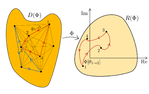
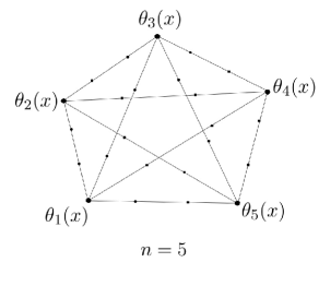
Figure 3: Network of test functions: A closed path in the function space $D(\Phi)$ made of four lines (e.g., the red polygon) is mapped through the functional $\Phi$ into a closed curve in the complex plane. Vertex and edges of the network are elements of $S_{2}^{(m)}$. We also show a complete graph with $n=5$ nodes, where each edge is discretized with $p=4$ points.

The function space $S_{q}^{(n)}$ admits a simple yet powerful graphical representation in terms of trajectories of functions [133, 215, 213, 214, 225]. To illustrate such representation, consider a complex-valued functional $\Phi$. A trajectory of functions in the space $D(\Phi)$ is a curve in $D(\Phi)$, which is mapped to a curve in $\mathbb{C}$ (see Figure 3). Furthermore, if the functional is continuous and differentiable, a smooth curve in $D(F)$ is mapped onto a smooth curve in $\mathbb{C}$. The set of trajectories in the complex plane associated with $S^{(m)}_{1}$ is shown in Figure 4. Each curve is parametrized by only one parameter $a_{j}$ and it cannot branch into two distinct curves . On the contrary, if we consider $S_{2}^{(m)}$ we are adding one more degree of freedom and each curve departing from $1$ can branch, but only once. Similarly, we can have three branches in $S_{3}^{(m)}$, etc. A remarkable distribution of nodes in $S_{2}^{(m)}$ is associated with networks of test functions, i.e., graphs in the function space $D(F)$. Vertex and edges are elements of $S_{2}^{(m)}$. A simple example is shown in Figure 3. In mathematics such network is called complete graph, i.e., an undirected graph in which every pair of distinct nodes is connected by a unique edge – the edge being the trajectory (straight line) of functions connecting $\theta_{i}$ to $\theta_{j}$. If we discretize each edge with $p$ collocation points (including the endpoints) and we have $m$ nodes then the number of degrees of freedom is $m(m-1)(p-2)/2+m$.

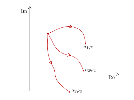
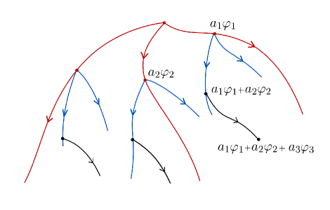
Figure 4: Trajectories in the range of a complex valued functional $\Phi$ corresponding to functions in the sets $S^{(m)}_{1}$ (left) and $S^{(m)}_{3}$ (right). In the case of $S^{(m)}_{1}$ each curve is parametrized by only one parameter $a_{j}$ and it cannot branch into two distinct curves. On the contrary, if we consider $S_{3}^{(m)}$ we are adding two more degrees of freedom and each curve can branch at most twice.

Another interesting set of interpolation nodes in $D(F)$ is the one obtained by setting all coefficients $a_{i_{p}}$ in (89) equal to $1$, i.e.,

$$\widehat{S}^{(m)}_{q}=\left\{\theta_{i}(x)\in D(F)\,\,|\,\,\theta_{i}(x)=\varphi_{i_{1}}(x)+\cdots+\varphi_{i_{q}}(x)\right\},\qquad i_{s}=0,...,m,$$ (91)

If the set $\{\varphi_{j}\}$ includes the null element $\{0\}$, then by symmetry (91) is equivalent to

$$\widehat{S}^{(m)}_{q}=\left\{\{0\},\{\varphi_{1},..,\varphi_{m}\},\{2\varphi_{1},..,2\varphi_{m}\},\{(\varphi_{1}+\varphi_{2}),...,(\varphi_{1}+\varphi_{m})\},\{(\varphi_{2}+\varphi_{3}),...,(\varphi_{2}+\varphi_{m})\},...\right\}.$$ (92)

In this case, the number of elements (cardinality) of $\widehat{S}^{(m)}_{q}$ is

$$\#\widehat{S}^{(m)}_{q}=\sum_{j=0}^{q}\binom{j+m-1}{j},\qquad\textrm{where}\,\,\,\binom{i}{j}\,\,\,\textrm{is the binomial coefficient.}$$ (93)

For example,

$$\#\widehat{S}^{(10)}_{1}=11,\qquad\#\widehat{S}^{(10)}_{2}=66\qquad\#\widehat{S}^{(10)}_{3}=286,\qquad\#\widehat{S}^{(10)}_{5}=3003,\qquad\#\widehat{S}^{(10)}_{10}=184756.$$ (94)

In addition, the cardinality of $\widehat{S}^{(m)}_{q}$ satisfies the recursion relation

$$\#\widehat{S}^{(m)}_{q}=\#\widehat{S}^{(m)}_{q-1}+\binom{q+m-1}{q}.$$ (95)

The set of functions $\widehat{S}^{(m)}_{q}$ is sufficient to uniquely identify a polynomial functional of order $q$ in which each kernel function is represented relative to tensor product basis with $m$ elements in each variable. However, $\widehat{S}^{(m)}_{q}$ is, in general, not sufficient to accurately interpolate nonlinear functionals. The main problem is that the set of nodes (91) may not be large enough or may not cover the function space $D(F)$ appropriately. Another open question is related to the selection of optimal interpolation nodes in $D(F)$ yielding highly accurate representations. This question is addressed in Section 3.4.1.

In a finite-dimensional setting, we can sample the coefficients $a_{i_{p}}$ in (89), e.g., at sparse grids locations [11, 24], thai is at unions of appropriate tensorizations of one-dimensional point sets such as Gauss-Hermite, Clenshaw-Curtis, Chebyshev or Leja [151]. This yields the set

$$\widetilde{S}^{(m)}_{q}=\left\{\theta_{i}(x)\in D(F)\,\,|\,\,\theta_{i}(x)=a_{i_{1}}\varphi_{i_{1}}(x)+\cdots+a_{i_{q}}\varphi_{i_{q}}(x)\right\},\qquad i_{s}=1,...,m,$$ (96)

where the vector $(a_{i_{1}},...,a_{i_{q}})$ takes discrete values at sparse grid nodes. As an example, in Figure 5 we plot three Clenshaw-Curtis grids and few samples of the corresponding interpolation nodes in $\widetilde{S}^{(2)}_{2}$. For illustration purposes, the basis elements $\varphi_{1}(x)$ and $\varphi_{2}(x)$ here are chosen as

$$\varphi_{1}(x)=\sin(x)e^{\cos(x)},\qquad\varphi_{2}(x)=\sin(2x)e^{\cos(2x)}.$$ (97)

    level 5                                          level 7                                          level 10

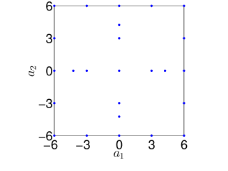
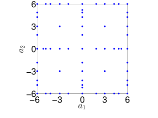
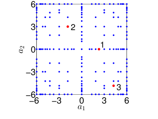
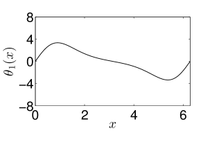
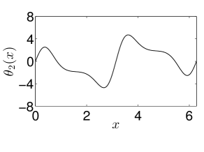
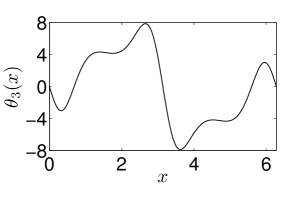
Figure 5: Clenshaw-Curtis point sets and corresponding nodes in $\theta_{i}(x)=a_{1_{i}}\varphi_{1}(x)+a_{2_{i}}\varphi_{2}(x)$ ($i=1,2,3$) in the test function space $\widetilde{S}^{2}_{2}$. Specifically, we plot $\theta_{i}(x)$ corresponding to the nodes $1$, $2$ and $3$ marked in red in the top right Figure. The basis elements $\varphi_{k}(x)$ here are chosen as $\sin(kx)\exp(\cos(kx))$ ($k=1,2$).

The construction of sparse grids usually follows the Smolyak algorithm. Other dimension-adaptive schemes and greedy Leja rules were recently proposed in [32, 151, 153].

3.2.2 Polynomial Interpolation of Nonlinear Functionals

Let $F:D(F)\rightarrow Y$ ($Y=\mathbb{R}$ or $\mathbb{C}$) be a nonlinear real- or complex-valued functional on $D(F)$. Consider the set of polynomial functionals of degree $n$

$$\Pi_{n}([\theta])=L_{0}+L_{1}([\theta])+L_{2}([\theta],[\theta])+\cdots+L_{n}([\theta],...,[\theta]),$$ (98)

where $L_{0}\in Y$, and $L_{k}:D(F)^{k}\rightarrow Y$ are $k$-linear symmetric functionals

$$L_{k}([\theta_{1}],...,[\theta_{p}])=\int\cdots\int K_{k}(x_{1},..,x_{k})\theta_{1}(x_{1})\cdots\theta_{k}(x_{k})dx_{1}\cdots dx_{k},\qquad k=1,...,n.$$ (99)

A comparison between equations (98) and (44) yields

$$P_{k}([\theta])=L_{k}([\theta],...,[\theta]),$$ (100)

and therefore we can equivalently write (98) as

$$\Pi_{n}([\theta])=\sum_{k=1}^{n}P_{k}([\theta]).$$ (101)

The symmetry assumption on $L_{k}$ implies that $K_{k}(x_{1},...,x_{k})$ are symmetric kernels, i.e., any permutation of $x_{1}$, …, $x_{n}$ leaves $K_{k}$ unchanged. It is obviously possible to define polynomial functionals with non-symmetric kernels. However, such functionals can be always written in a symmetric form by rearranging the kernel functions appropriately. For example, let $H_{2}(x_{1},x_{2})$ be non-symmetric. It is easy to verify that

$$\int_{a}^{b}\int_{a}^{b}H_{2}(x_{1},x_{2})\theta(x_{1})\theta(x_{2})dx_{1}dx_{2}=\int_{a}^{b}\int_{a}^{b}K_{2}(x_{1},x_{2})\theta(x_{1})\theta(x_{2})dx_{1}dx_{2},\qquad\forall\theta\in D(F),$$ (102)

where

$$K_{2}(x_{1},x_{2})=\frac{1}{2}\left(H_{2}(x_{1},x_{2})+H_{2}(x_{2},x_{1})\right).$$ (103)

In other words, the value of the integral does not change if we replace $H_{2}(x_{1},x_{2})$ with its symmetrized version $K_{2}(x_{1},x_{2})$. More generally, we can symmetrize any kernel $H_{p}(x_{1},...,x_{p})$ by summing up all terms corresponding to all possible permutations of $(x_{1},...,x_{p})$ and then dividing up by the factorial of $p$. For example,

$$K_{3}(x_{1},x_{2},x_{3})=\frac{1}{3!} \left(H_{3}(x_{1},x_{2},x_{3})+H_{3}(x_{1},x_{3},x_{2})+H_{3}(x_{2},x_{1},x_{3})+H_{3}(x_{2},x_{3},x_{1})+\right.$$

$$\left.H_{3}(x_{3},x_{1},x_{2})+H_{3}(x_{3},x_{2},x_{1})\right).$$ (104)

The symmetry of the operators $L_{k}$ significantly reduces the number of collocation nodes in the function space $D(F)$ needed to identify kernels $K_{k}$, provided these are of finite-rank.

The polynomial functional interpolation problem can be stated as follows: Given a set of $m$ nodes $\{\theta_{1}(x),...,\theta_{m}(x)\}$ in $D(F)$, find a polynomial functional in the form (98) satisfying the interpolation conditions

$$\Pi_{n}([\theta_{i}])=F([\theta_{i}]),\qquad i=1,...,m.$$ (105)

The Stone-Weierstrass Approximation Theorem

The possibility of approximating an arbitrary continuous functional in Hilbert or Banach spaces in terms polynomial functionals is justified by theorems analogous to the classical Weierstrass theorem for continuous functions. We recall that such theorem states that if $f(x)$ is a continuous, real-valued function on the closed interval $[a,b]$, then given any $\epsilon>0$ there exists a real polynomial $p(x)$ such that $|f(x)-p(x)|<\epsilon$ for all $x\in[a,b]$. A remarkable generalization of this result has its roots in the Stone-Weierstrass theorem [210], which can be stated as follows: suppose that $X$ is a compact metric space and $K$ is an algebra of continuous, real-valued functions on $X$ that separates points. Then for any continuous, real-valued functional $F$ on $X$ and for any $\epsilon>0$ there exists a polynomial functional $\Pi\in K$ such that $\left\|F([u])-\Pi([u])\right\|<\epsilon$ for all $u\in X$. The first paper dealing with this subject is due Frechét [65]. He showed that any continuous functional can be represented by a series of polynomial functionals whose convergence is uniform in all compact sets of continuous functions. This result was generalized to compact sets of functions in Hilbert and Banach spaces by Prenter [182] and Istratescu [94], respectively. Other relevant work in this area is [70, 180, 17, 28, 170, 178].

3.2.3 Porter Interpolants

An effective way to construct finite-order polynomial functionals with minimal norm interpolating arbitrary continuous functionals in Hilbert spaces was proposed by W. Porter in [179]. The key idea relies on minimizing the norm of (98) subject to the interpolation conditions (105). A natural way to impose such conditions is through Lagrange multipliers. This yields the variational principle

$$\min_{K_{1},..,K_{n}}\left\|\Pi_{n}\right\|^{2}+\sum_{j=1}^{m}\lambda_{i}\left(\Pi_{n}([\theta_{i}])-F([\theta_{i}])\right),$$ (106)

The minimum is relative to arbitrary variations of the kernel functions $K_{j}(x_{1},...,x_{j})$. Also, $\left\|\Pi_{n}\right\|^{2}$ is the norm of the polynomial functional (98), which is defined as

$$\left\|\Pi_{n}\right\|^{2}=\sum_{p=0}^{n}\int\cdots\int\left|K_{p}(x_{1},...,x_{p})\right|^{2}dx_{1}\cdots dx_{p}<\infty$$ (107)

The solution to the variational principle (106) allows us to identify the kernel functions $K_{j}(x_{1},...,x_{j})$ and, correspondingly, the polynomial functional with minimal norm interpolating $F([\theta])$ at the $m$ nodes $\{\theta_{1},...,\theta_{m}\}$. Specifically, we obtain

$$K_{p}(x_{1},...,x_{p})=\sum_{j,k=1}^{m}\pi^{(p)}_{j}(x_{1},..,x_{p})H^{-1}_{jk}F([\theta_{k}]),\qquad i=0,...,n.$$ (108)

In this equation,

$$\pi^{(0)}_{j}=1,\qquad\pi^{(p)}_{j}(x_{1},..,x_{p})=\theta_{j}(x_{1})\cdots\theta_{j}(x_{p})\qquad p=1,2,...$$ (109)

while the (symmetric) matrix $H_{ij}$ is defined as

$$H_{ij}=1+\left(\theta_{i},\theta_{j}\right)+\left(\theta_{i},\theta_{j}\right)^{2}+\cdots+\left(\theta_{i},\theta_{j}\right)^{n},$$ (110)

where $(,)$ denotes the $L_{2}(V)$ inner product, $V$ being the domain of the interpolation nodes $\theta_{j}(x)$. The polynomial functional $\Pi_{n}$ constructed in this way exists if $F([\theta_{k}])$ is in the range of the matrix $\bm{H}$ (see [179] for further details). If one wants to approximate $F([\theta])$ in terms of a superimposition of monomials with orders defined by an index set $\mathcal{I}$ then

$$H_{ij}=\sum_{p\in\mathcal{I}}\left(\theta_{i},\theta_{j}\right)^{p}$$ (111)

The total degree of the polynomial functional is the largest number in the index set $\mathcal{I}$. It is convenient to write Porter’s interpolant in terms of basis functionals $g_{i}([\theta])$ as

$$\Pi_{n}\left([\theta]\right)=\sum_{k=1}^{m}F\left([\theta_{k}]\right)g_{k}([\theta]),$$ (112)

where

$$g_{k}([\theta])=\sum_{j=1}^{m}H_{jk}^{-1}\sum_{p\in\mathcal{I}}\left(\theta_{j},\theta\right)^{p}.$$ (113)

The functional interpolant (112)-(113) has the following properties:

1. $\{g_{k}([\theta])\}$ is a set of cardinal basis functionals, i.e., $g_{k}([\theta_{q}])=\delta_{kq}$. This implies that Porter’s interpolant is a cardinal Lagrangian interpolant.

2. If the interpolation nodes $\{\theta_{1},...,\theta_{m}\}$ are orthonormal with respect to the inner product $(,)$ then $H_{ii}=\#\mathcal{I}$ (cardinality of the index set $\mathcal{I}$) and $H_{ij}$ ($i\neq j$) either equal to one or zero, depending on whether we have $\{0\}$ in the set $\mathcal{I}$ or not. In every case, $\bm{H}$ is a matrix with diagonal entries equal to $\#\mathcal{I}$ and off-diagonal entries equal to wither zero or one. Such matrix is always invertible provided $\mathcal{I}$ does not reduce to the single element $\{0\}$.

3. Porter’s interpolant is degenerate for $\mathcal{I}=\{0\}$ as the matrix $\bm{H}$ is rank one and therefore it is not invertible. The Moore-Penrose pseudoinverse $\bm{H}^{+}$, however, exists and it provides the correct form of the interpolant. To show this in a simple case, consider the constant functional $F([\theta])=c\in\mathbb{R}$ and the zero-order polynomial interpolant at $\{\theta_{1},...,\theta_{m}\}$

   $$\Pi_{0}([\theta])=K_{0}=\sum_{k,j=1}^{m}H^{-1}_{jk}F([\theta_{j}]).\qquad H_{ij}=1.$$ (114)

   Clearly, $H^{-1}_{jk}$ does not exist since $H_{ij}=1$ and therefore $\textrm{rank}(H)=1$. However, the Moore-Penrose pseudoinverse of $\bm{H}$ has components $H^{+}_{ij}=1/m^{2}$, and therefore $\Pi_{0}([\theta])=c=F([\theta])$.

4. The polynomial functional (112)-(113) is an interpolant if and only if the matrix (111) is invertible, i.e., full rank. This depends on both the choice of interpolation nodes and on the index set $\mathcal{I}$. The Moore-Penrose pseudoinverse $\bm{H}^{+}$, in general, does not allow to satisfy the interpolation condition. Indeed, by evaluating (112) at the interpolation nodes $\theta_{k}$ we obtain

   $$\Pi_{n}\left([\theta_{i}]\right)=\sum_{k=1}^{m}F\left([\theta_{k}]\right)\sum_{j=1}^{m}H_{jk}^{-1}H_{ji}=F([\theta_{i}]).$$ (115)

   However, if we replace $H_{jk}^{-1}$ with $H_{jk}^{+}$ then we get $\Pi_{n}\left([\theta_{i}]\right)\neq F\left([\theta_{i}]\right)$, since $\bm{H}^{+}\bm{H}\neq\bm{I}$.

5. Consider the approximation of constant functionals $F([\theta])=c$ by polynomial functionals of order one, i.e., $\Pi_{1}([\theta])=L_{0}+L_{1}([\theta])$. Assume that the interpolation nodes $\{\theta_{k}\}_{k=1,...,m}$ are orthogonal functions with norm that decreases with $m$ as $1/m$ (see Section 6.1). Let $H_{ij}=1+h\delta_{ij}$ where $h=\left\|\theta_{j}\right\|^{2}$ be the matrix (111) corresponding to the index set $\mathcal{I}=\{0,1\}$. By using the identity

   $$\lim_{h\rightarrow 0}\frac{1}{h}\left(1+h\delta_{ij}\right)^{-1}=\delta_{ij}-\frac{1}{m}$$ (116)

   we obtain

   $$\Pi_{1}([\theta])\simeq c\sum_{k,j=1}^{m}\left(h\delta_{jk}-\frac{h}{m}\right)\left(1+(\theta,\theta_{j})\right)\qquad\textrm{as}\qquad h\rightarrow 0\quad\textrm{and}\quad m\rightarrow\infty.$$ (117)

   This means that $\displaystyle\lim_{m\rightarrow\infty}\Pi_{1}([\theta])=c$, i.e., the polynomial interpolant is consistent with the functional $F$ in the sense that the linear term becomes smaller and smaller as we increase the number of test functions $\theta_{k}$. In the limit $m\rightarrow\infty$ (infinite number of test functions) we see the linear term is absent, and we correctly recover the constant functional.

By extending these arguments to higher-order polynomial functionals in Hilbert spaces, one can show that Porter’s interpolants of order $n$ converge pointwise to entire functionals or any polynomial functional of order $n$ or less as the number of interpolation nodes $\theta_{k}$ goes to infinity (see [105] and Theorem 1 in [103]).

Functional Derivatives

The functional derivatives of Porter interpolants can be easily determined by computing the functional derivatives of the basis functionals $g_{i}([\theta])$ defined in (113). To this end, we first notice that

$$\frac{\delta(\theta,\theta_{k})^{p}}{\delta\theta(x)}=(\theta,\theta_{k})^{p-1}p\theta_{k}(x),\qquad p\geq 1.$$ (118)

A substitution of this formula into (113) yields

$$\frac{\delta g_{k}([\theta])}{\delta\theta(x)}=\sum_{j=1}^{m}\theta_{j}(x)H_{jk}^{-1}\sum_{p\in\mathcal{I}}\left(\theta_{j},\theta\right)^{p-1}p$$ (119)

By evaluating $g_{k}([\theta])$ at the nodes $\theta_{j}(x)$ we obtain a functional generalization of the classical differentiation matrix [84]

$$D^{(1)}_{ji}(x)=\frac{\delta g_{i}([\theta_{j}])}{\delta\theta(x)}.$$ (120)

Similarly, the second-order functional derivative of $g_{k}([\theta])$ is

$$\frac{\delta^{2}g_{k}([\theta])}{\delta\theta(x)\delta\theta(y)}=\sum_{j=1}^{m}\theta_{j}(x)\theta_{j}(y)H_{jk}^{-1}\sum_{p\in\mathcal{I}}p(p-1)\left(\theta_{j},\theta\right)^{p-2},$$ (121)

and it yields the following second-order functional differentiation matrix

$$D^{(2)}_{ji}(x,y)=\frac{\delta^{2}g_{i}([\theta_{j}])}{\delta\theta(x)\delta\theta(y)}.$$ (122)

At this point it is useful to provide simple examples of functional interpolation in Hilbert spaces. Example 1: Consider the first-order polynomial functional

$$P_{1}([\theta])=\int_{a}^{b}K_{1}(x)\theta(x)dx.$$ (123)

To represent $P_{1}([\theta])$ in terms of a functional interpolant it is sufficient to consider the set of orthonormal functions $\widehat{S}^{(m)}_{1}=\{\varphi_{1},...,\varphi_{m}\}$ (see Eq. (91)). In this case, Porter’s cardinal basis functionals (113) reduce to

$$g_{i}([\theta])=\left(\varphi_{i},\theta\right),$$ (124)

and the functional interpolant can be written as

$$\Pi_{1}([\theta])=\sum_{i=1}^{m}P_{1}([\varphi_{i}])g_{i}([\theta]).$$ (125)

Clearly, we have that $\Pi_{1}([\theta])\rightarrow P_{1}$ as $m\rightarrow\infty$.

Example 2: Consider the second-order polynomial functional

$$P_{2}([\theta])=\int_{a}^{b}\int_{a}^{b}K_{2}(x,y)\theta(x)\theta(y)dxdy.$$ (126)

To represent $P_{2}([\theta])$ in terms of a functional interpolant it is sufficient to consider the set of orthonormal functions

$$\hat{\hat{S}}^{(m)}_{2}=\{\varphi_{1},...,\varphi_{m},(\varphi_{1}+\varphi_{2}),...,(\varphi_{1}+\varphi_{m}),(\varphi_{2}+\varphi_{3}),...,(\varphi_{2}+\varphi_{m}),...\}$$ (127)

which is similar (but not equal) to (91). The matrix (111) associated with this set has the structure shown in Figure 6.

           $\hat{\hat{S}}^{(10)}_{1}$                                                       $\hat{\hat{S}}^{(10)}_{2}$                                                        $\hat{\hat{S}}^{(10)}_{3}$

Figure 6: Structure of the $H$-matrix (111) associated with the function set $\hat{\hat{S}}^{(10)}_{1}$, $\hat{\hat{S}}^{(10)}_{2}$ and $\hat{\hat{S}}^{(10)}_{3}$ defined in Eq. (127). We consider $\mathcal{I}=1$, $\mathcal{I}=2$ and $\mathcal{I}=3$, respectively.

The cardinal basis functionals (113) reduce to

$$g_{k}([\theta])=\sum_{j=1}^{\#\hat{\hat{S}}^{(m)}_{2}}H_{jk}^{-1}\left(\theta_{j},\theta\right)^{2},$$ (128)

where $\#\hat{\hat{S}}^{(m)}_{2}$ is the number of elements of $\hat{\hat{S}}^{(m)}_{2}$, $\theta_{k}=\varphi_{k}$ ($k=1,...,m$), $\theta_{m+1}=\varphi_{1}+\varphi_{2}$, etc. The functional interpolant can be written as

$$\Pi_{2}([\theta])=\sum_{i=1}^{\#\hat{\hat{S}}^{(m)}_{2}}P_{2}([\theta_{i}])g_{i}([\theta]),$$ (129)

and it converges $P_{2}$ as $m\rightarrow\infty$ (see Section 6).

Example 3: Consider the third-order polynomial functional

$$P_{3}([\theta])=\int_{a}^{b}\int_{a}^{b}\int_{a}^{b}K_{3}(x_{1},x_{2},x_{3})\theta(x_{1})\theta(x_{2})\theta(x_{3})dx_{1}dx_{2}dx_{3}.$$ (130)

To represent $P_{3}([\theta])$ in terms of a functional interpolant it is sufficient to consider the set of functions $\hat{\hat{S}}^{(m)}_{3}\subset\hat{S}^{(m)}_{3}$ defined as

$$\hat{\hat{S}}^{(m)}_{3}=\hat{\hat{S}}^{(m)}_{2}\cup\{(\varphi_{i}+\varphi_{j}+\varphi_{k}),\quad k>j>i\}$$ (131)

where $\hat{\hat{S}}^{(m)}_{2}$ is as in (127). The matrix (111) associated with this set has the structure shown in Figure 6 The cardinal basis functionals (113) reduce to

$$g_{k}([\theta])=\sum_{j=1}^{\#\hat{\hat{S}}^{(m)}_{3}}H_{jk}^{-1}\left(\theta_{j},\theta\right)^{3}.$$ (132)

The functional interpolant can be written as

$$\Pi_{3}([\theta])=\sum_{i=1}^{\#\widehat{S}^{(m)}_{3}}P_{3}([\theta_{i}])g_{i}([\theta]).$$ (133)

More-Penrose Pseudoinverse and Non-Cardinal Basis Functionals

We emphasized that the matrix $H_{ij}$ defined in (111) may be not invertible in some cases. This happens, for example, if the interpolation nodes $\theta_{k}(x)$ are linearly dependent or if there exist a symmetry such the inner product of $\theta_{k}$ and $\theta_{j}$ yields linearly dependent rows/columns in (111). In this cases we can still construct a polynomial functional with minimal norm which, however, does not interpolate $F$ at $\theta_{k}$. To this end, we simply use the Moore-Penrose pseudoinverse of $H_{ij}$ to obtain a representation of Porter’s polynomial functionals in terms of a non-cardinal basis $g^{+}_{k}([\theta])$ as

$$\Pi_{n}\left([\theta]\right)=\sum_{k=1}^{m}F\left([\theta_{k}]\right)g^{+}_{k}([\theta]).$$ (134)

where

$$g^{+}_{k}([\theta])=\sum_{j=1}^{m}H_{jk}^{+}\sum_{p\in\mathcal{I}}\left(\theta_{j},\theta\right)^{p}.$$ (135)

In the last equation $H_{ij}^{+}$ denotes the Moore-Penrose pseudoinverse of $H_{ij}$. The approximation properties of polynomial functionals in the form (134) will be studied in Section 6.3.2 and Section 6.4.

Recursive Porter Interpolation

The number of interpolation nodes $\theta_{k}$ required to represent exactly a polynomial functional of order $n$ is given in (93). For example, if we set $m=10$ elementary functions and polynomial order $n=12$ such formula yields $646646$ interpolation nodes! Such large number of nodes may be an issue when computing Porter’s interpolants. In fact, computing the inverse of (111) rapidly becomes intractable as we increase either $m$ or $n$. To overcome this problem we can split the process of inverting the matrix (111) into a recursive algorithm, e.g., by using Schur complements and blockwise inversion. To this end, consider the set of nodes

$$\left\{\{\theta_{1},...,\theta_{m}\},\{\theta_{m+1},...,\theta_{2m}\},\{\theta_{2m+1},...,\theta_{3m}\},...,\{\theta_{(N-1)m+1},...,\theta_{Nm}\}\right\},$$ (136)

and define the matrices

$$H^{(I,J)}_{ij}=\sum_{p\in\mathcal{I}}(\theta_{i},\theta_{j})^{p}\qquad i=(I-1)m+1,..,Im\quad j=(J-1)m+1,..,Jm,$$ (137)

where $\mathcal{I}$ denotes the index set of Porter’s monomials while $I$ and $J$ run from $1$ to $N$. The $H$-matrix (111) corresponding to the set (136) can be represented in a block-wise form as

$$H_{N}=\left[\begin{array}[]{ccc}H^{(1,1)}&\cdots&H^{(1,N)}\\ \vdots&&\vdots\\ H^{(N,1)}&\cdots&H^{(N,N)}\\ \end{array}\right].$$ (138)

The computational cost of inverting such matrix is prohibitive if $Nm$ is large. However, we can use the following recursive procedure. We first build and invert $H_{1}=H^{(1,1)}$, corresponding to the first set of $m$. This allows us to determine Porter’s interpolant on the first set of $m$ nodes in (136). Next we add the second set, i.e., the nodes $\{\theta_{m+1},...,\theta_{2m}\}$. The matrix (111) corresponding to the nodal set $\{\theta_{1},...,\theta_{2m}\}$ is

$$H_{2}=\left[\begin{array}[]{cc}H_{1}&C_{1}\\ C_{1}^{T}&H^{(2,2)}\\ \end{array}\right]\qquad C_{1}=H^{(1,2)}$$ (139)

and it can be inverted by using the block-wise formula [142]

$$H^{-1}_{2}=\left[\begin{array}[]{cc}H_{1}^{-1}+B_{1}A_{1}B_{1}^{T}&-B_{1}A_{1}\\ -A_{1}B_{1}&A_{1}\\ \end{array}\right]$$ (140)

where

$$B_{1} =H_{1}^{-1}C_{1},$$ (141)

$$A_{1} =\left(H^{(2,2)}-C_{1}^{T}B_{1}\right)^{-1}\qquad\textrm{(inverse of the Schur complement)}.$$ (142)

Now we bring in the third set of nodes $\{\theta_{2m+1},...,\theta_{3m}\}$. The matrix (111) corresponding to the nodal set $\{\theta_{1},...,\theta_{3m}\}$ is

$$H_{3}=\left[\begin{array}[]{cc}H_{2}&C_{2}\\ C_{2}^{T}&H^{(3,3)}\\ \end{array}\right]\qquad C_{2}=\left[\begin{array}[]{c}H^{(1,3)}\\ H^{(2,3)}\end{array}\right],$$ (143)

and its inverse is, as before,

$$H^{-1}_{3}=\left[\begin{array}[]{cc}H_{2}^{-1}+B_{2}A_{2}B_{2}^{T}&-B_{2}A_{2}\\ -A_{2}B_{2}&A_{2}\\ \end{array}\right]$$ (144)

where

$$B_{2}=H_{2}^{-1}C_{2},\qquad A_{2}=\left(H^{(3,3)}-C_{2}^{T}B_{2}\right)^{-1}.$$ (145)

At this point it is clear that the procedure can be iterated as many times as needed. This generates a sequence of basis functionals (113), and an interpolating polynomial functional with minimal norm that passes through an increasing number of nodes. In this way, we have reduced the problem of computing Porter’s interpolant through a very large number of nodes into a sequence of matrix inversions of dimension at most $m\times m$. The storage requirements of the algorithm just described, however, is not small as because Porter’s basis functionals are ultimately defined by $H_{N}^{-1}$. An open question is the identification of interpolation nodes $\theta_{j}$ leading to minimal complexity/storage requirements for $H_{N}^{-1}$.

An alternative interpolation method makes use of residuals. The main idea is sketched in Figure 7.

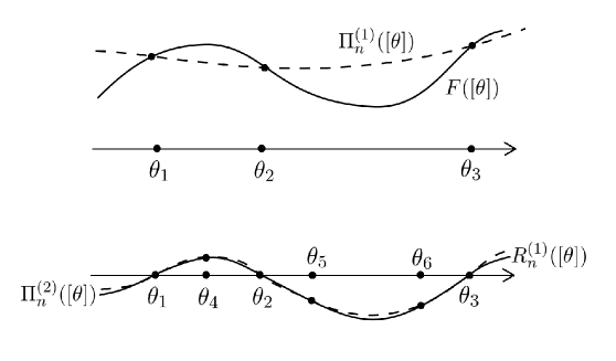
Figure 7: Recursive polynomial interpolation: Minimal residual approach.

The functional $F([\theta])$ is interpolated by a polynomial of order $n$, denoted as $\Pi^{(1)}_{n}([\theta])$, at just three nodes $\{\theta_{1},\theta_{2},\theta_{3}\}$. Subtracting $\Pi^{(1)}_{n}([\theta])$ from $F([\theta])$ yields the functional residual

$$R^{(1)}_{n}([\theta])=F([\theta])-\Pi^{(1)}_{n}([\theta])$$ (146)

which is zero at $\theta_{1}$, $\theta_{2}$ and $\theta_{3}$ because of the interpolation condition. Now we add three more nodes $\{\theta_{4},\theta_{5},\theta_{6}\}$ and construct a Porter’s interpolant of $R^{(1)}_{n}([\theta])$ at $\{\theta_{1},...,\theta_{6}\}$. We denote such interpolant by $\Pi^{(2)}_{n}([\theta])$. The computation of $\Pi^{(2)}_{n}([\theta])$ can be carried out as above by using Schur complements and block-wise inversion of (111). The polynomial functional $\Pi^{(1)}_{n}([\theta])+\Pi^{(2)}_{n}([\theta])$ interpolates $F([\theta])$ at $\{\theta_{1},...,\theta_{6}\}$. The recursive construction proceeds with the definition of the new residual

$$R^{(2)}_{n}([\theta])=F([\theta])-\Pi^{(1)}_{n}([\theta])-\Pi^{(2)}_{n}([\theta]),$$ (147)

three more nodes $\{\theta_{7},\theta_{8},\theta_{9}\}$, and a Porter’s polynomial $\Pi^{(3)}_{n}([\theta])$, interpolating $R^{(2)}_{n}([\theta])$ at $\{\theta_{1},...,\theta_{9}\}$. Proceeding recursively with higher-order residuals up to order $r$, we obtain the polynomial functional

$$Q_{n}([\theta])=\sum_{k=1}^{r}\Pi^{(k)}_{n}([\theta]).$$ (148)

Clearly $Q_{n}([\theta])$ interpolates $F([\theta])$ at all nodes $\theta_{k}$ and therefore it is completely equivalent to $\Pi_{n}([\theta])$, i.e., $Q_{n}([\theta])=\Pi_{n}([\theta])$.

Hierarchical Matrices

The algorithm we just described aim at reducing the computational cost of computing polynomial functional interpolants by inverting the matrix $\bm{H}$ defined in (111) in a block-wise fashion or recursively. The structure of such matrix obviously depends on how we select the interpolation nodes in the function space $D(F)$. An interesting open question is whether we can determine sets of nodes for which the interpolation problem can be solved at a minimal cost. Stated in matrix terms, can we identity sets of nodes yielding structured matrices that can be easily inverted, e.g., hierarchical matrices? The matrices shown in Figure 6 have indeed a self similar structure which can be used to speed up their inversion. We leave this question open for future research. For uniquely solvable interpolation problems we could equivalently construct Khlobystov polynomial functionals (see Section 3.2.5), and determine the coefficients of the expansion by using the method of moments.

3.2.4 Prenter Interpolants

Another method to determine polynomial interpolants in Hilbert and Banach spaces was introduced by Prenter in [183]. She proved that if $F([\theta])$ is a functional in a Hilbert space $D(F)$, and $\theta_{j}\in D(F)$ are interpolation nodes, then there exists a $n$th-order functional interpolant in the form

$$\Pi_{n}([\theta])=\sum_{i=1}^{n}F([\theta_{i}])g_{i}([\theta]),$$ (149)

where

$$g_{i}([\theta])=\prod_{\begin{subarray}{c}j=1\\ j\neq i\end{subarray}}^{n}\frac{\left(\theta-\theta_{j},\theta_{i}-\theta_{j}\right)}{\left(\theta_{i}-\theta_{j},\theta_{i}-\theta_{j}\right)}\qquad\textrm{(cardinal basis)}.$$ (150)

As before, $(,)$ denotes the inner product in $L_{2}(V)$, where $V$ is the domain of $\theta_{k}(x)$. Note that each basis element $g_{i}([\theta])$ is a polynomial functional of order $n$. On the other hand, Porter’s method yields polynomial basis functionals of total degree $\max(\mathcal{I})$, where the index set $\mathcal{I}$ does not depend on the number of collocation points. Porter [178] applied Prenter’s theorems to causal systems, while Bertuzzi, Gandolfi and Germani [16, 17] extended Prenter’s results to causal approximation of input-output maps in Hilbert spaces. Generalizations to Banach spaces can be found in Chapter 3 of [216] (see also [134] and the references therein). The functional derivatives of Prenter’s polynomial functionals can be obtained by computing the functional derivatives of (150). This yields

$$\frac{\delta g_{i}([\theta])}{\delta\theta(x)}=\sum_{\begin{subarray}{c}k=1\\ k\neq i\end{subarray}}^{n}\frac{\theta_{i}(x)-\theta_{k}(x)}{\left\|\theta_{i}-\theta_{k}\right\|^{2}}g_{ik}([\theta]),$$ (152)

$$\frac{\delta^{2}g_{i}([\theta])}{\delta\theta(x)\delta\theta(y)}=\sum_{\begin{subarray}{c}k=1\\ k\neq i\end{subarray}}^{n}\frac{\theta_{i}(x)-\theta_{k}(x)}{\left\|\theta_{i}(x)-\theta_{k}(x)\right\|^{2}}\sum_{\begin{subarray}{c}s=1\\ s\neq k\end{subarray}}^{n}\frac{\theta_{i}(y)-\theta_{s}(y)}{\left\|\theta_{i}(y)-\theta_{s}(y)\right\|^{2}}g_{iks}([\theta]),$$ (153)

where

$$g_{ik}([\theta])=\prod_{\begin{subarray}{c}j=1\\ j\neq i,k\end{subarray}}^{n}\frac{(\theta-\theta_{j},\theta_{i}-\theta_{j})}{\left\|\theta_{i}-\theta_{j}\right\|^{2}},\qquad g_{iks}([\theta])=\prod_{\begin{subarray}{c}j=1\\ j\neq i,k,s\end{subarray}}^{n}\frac{(\theta-\theta_{j},\theta_{i}-\theta_{j})}{\left\|\theta_{i}-\theta_{j}\right\|^{2}}.$$ (154)

Note that the functional derivatives (152)-(153) are more complicated than the ones we obtained in the case Porter’s basis (119). As noted by Allasia and Bracco in [4], Prenter’s interpolants are badly conditioned as the number of interpolation nodes in function space increases. This unfortunate feature is common to many Lagrange interpolants.

3.2.5 Khlobystov Interpolants

We have seen that any continuous functional in a Hilbert or a Banach space can be approximated uniformly in terms of polynomial functionals [181, 17, 94, 134, 92, 216]. Such polynomial functionals may be built based on an interpolation process (see Section 3.2.3 and Section 3.2.4). What are the convergence properties of such expansions? To address this question, let us consider a polynomial interpolation problem of a given polynomial functional $\Pi_{n}([\theta])$ in the form (101). Assume that $D(\Pi_{n})$ is a Hilbert space of test functions, introduce the orthonormal basis $\{\varphi_{1},...,\varphi_{m}\}$ in $D(\Pi_{n})$, and consider the following expansion

$$\Pi^{I}_{n}([\theta])=\sum_{k=1}^{n}\sum_{i_{1}=1}^{m}\cdots\sum_{i_{k}=1}^{m}(\theta,\varphi_{i_{1}})\cdots(\theta,\varphi_{i_{k}})a_{k}(\varphi_{i_{1}},...,\varphi_{i_{k}}),$$ (155)

where $(,)$ is an inner product in $D(\Pi_{n})$ and $a_{k}(\varphi_{i_{1}},...,\varphi_{i_{k}})$ are real- or complex-valued coefficients. Clearly $\Pi^{I}_{n}([\theta])$ is an interpolant of $\Pi_{n}([\theta])$ at $\varphi_{k}$, i.e.,

$$\Pi^{I}_{n}([\varphi_{k}])=\Pi_{n}([\varphi_{k}]).$$ (156)

The next step is to write the coefficients $a_{k}(\varphi_{i_{1}},...,\varphi_{i_{k}})$ in terms of $\Pi_{n}([\varphi_{j}])$. To this end, we can use the method for finding orthonormal moments of regular polynomial functionals (Theorem 1 in [102]). This yields

$$n!a_{n}(\varphi_{i_{1}},...,\varphi_{i_{n}})= \Pi_{n}([\varphi_{i_{1}}+\cdots+\varphi_{i_{n}}])-\left\{\Pi_{n}([\varphi_{i_{1}}+\cdots+\varphi_{i_{n-1}}])+\right.$$

$$\left.\Pi_{n}([\varphi_{i_{1}}+\cdots+\varphi_{i_{n-2}}+\varphi_{i_{n}}])+\cdots+\Pi_{n}([\varphi_{i_{2}}+\cdots+\varphi_{i_{n}}])\right\}+$$

$$\left\{\Pi_{n}([\varphi_{i_{1}}+\cdots+\varphi_{i_{n-2}}])+\Pi_{n}([\varphi_{i_{1}}+\cdots+\varphi_{i_{n-3}}+\varphi_{i_{n-1}}])+\cdots+\right.$$

$$\left.\Pi_{n}([\varphi_{i_{3}}+\cdots+\varphi_{i_{n}}])\right\}\cdots+(-1)^{n-1}\left\{\Pi_{n}([\varphi_{i_{1}}])+\cdots+\Pi_{n}([\varphi_{i_{n}}])\right\}+$$

$$(-1)^{n}\Pi_{n}([0]).$$ (157)

Once $a_{n}(\varphi_{i_{1}},...,\varphi_{i_{n}})$ are available, we can construct the polynomial

$$\Pi_{n}-a_{n}(\varphi_{i_{1}},...,\varphi_{i_{n}})\prod_{z=1}^{n}(\theta,\varphi_{i_{z}})$$

and apply (157) again to determine $a_{n-1}(\varphi_{i_{1}},...,\varphi_{i_{n-1}})$. After $n$ iterations, we have available all coefficients to construct the polynomial functional (155). It was shown in [102] (Theorem 2) that the following error estimate holds

$$\left\|\Pi^{I}_{n}([\theta])-\Pi_{n}([\theta])\right\|\leq\sum_{k=1}^{n}\left\|P_{k}\right\|\left[\left(\left\|\theta\right\|+\epsilon_{m}([\theta])\right)^{k}-\left\|\theta\right\|^{k}\right],$$ (158)

where

$$\left\|P_{k}\right\|=\int\cdots\int\left|K_{k}(x_{1},...,x_{k})\right|dx_{1}\cdots dx_{k},$$ (159)

$$\epsilon_{m}([\theta])=\left\|\theta-\sum_{k=1}^{m}(\theta,\varphi_{k})\varphi_{k}\right\|.$$ (160)

This means that the interpolant (155) converges pointwise to the polynomial functional $\Pi_{n}([\theta])$ in (98) as the number of nodes $\{\varphi_{k}\}$ in the function space $D(\Pi_{n})$ goes to infinity. As noted by Khlobystov in [103], Porter’s interpolant (112) can be written exactly in the form (155) if we consider test functions in the form $\theta_{i}=\varphi_{i_{1}}+...+\varphi_{i_{n}}$ (see Lemma 1 in [103]). In this sense, Porter’s interpolants represent the Lagrangian form of Khlobystov’s interpolants. An interesting and very important question is the approximation of polynomial functionals of order $n$ in terms interpolants over nodal sets $\widehat{S}^{(m)}_{q}$, with $q<n$ (see Eq. (91)). A specific example would be the approximation of $P_{3}([\theta])$ in (130) by using an interpolant built on the set of nodes $\widehat{S}^{(m)}_{1}$. In some very special cases we may get uniform convergence as $m\rightarrow\infty$, for example when $K_{3}$ is diagonal

$$K_{3}(x_{1},x_{2},x_{3})=\sum_{j=1}^{m}a_{j}\varphi_{j}(x_{1})\varphi_{j}(x_{2})\varphi_{j}(x_{3}).$$ (161)

However, this won’t happen in general, and therefore we will have to accept a systematic truncation error in representing continuous nonlinear functionals. Such error is similar the error committed when we approximate infinite-variate functions, e.g., by second-order HDMR [237] (see Section 3.5).

Khlobystov interpolants with Hilbert-Schmidt Kernels

In this Section we present a procedure to construct interpolants of polynomial operators in Hilbert spaces with separable kernels. To this end, let us consider an orthonormal basis $\{\varphi_{1},\varphi_{2},...,\varphi_{m}\}$ and represent each kernel in (99) as

$$K_{1}(x_{1})= \sum_{i=1}^{m}a_{i}\varphi_{i}(x),$$ (162)

$$K_{2}(x_{1},x_{2})= \sum_{i,j=1}^{m}a_{ij}\varphi_{i}(x_{1})\varphi_{j}(x_{2}),$$ (163)

$$K_{3}(x_{1},x_{2},x_{3})= \sum_{i,j,k=1}^{m}a_{ijk}\varphi_{i}(x_{1})\varphi_{j}(x_{2})\varphi_{k}(x_{3}),$$ (164)

$$\cdots.$$

Without loss of generality we can assume that $K_{2}$, $K_{3}$, … are symmetric, i.e., that the coefficients $a_{ijk\cdots}$ are invariant under any permutation of the indices $i$, $j$, $k$, etc. A substitution of (162), (163), etc., into (98) yields the polynomial functional

$$\Pi_{n}([\theta])=K_{0}+\sum_{i=1}^{m}a_{i}(\varphi_{i},\theta)+\sum_{i,j=1}^{m}a_{ij}(\varphi_{i},\theta)(\varphi_{j},\theta)+\sum_{i,j,k=1}^{m}a_{ijk}(\varphi_{i},\theta)(\varphi_{j},\theta)(\varphi_{k},\theta)+\cdots.$$ (165)

At this point we pose the following question: How many interpolation nodes do we need to identify the coefficients $a_{i}$, $a_{ij}$, $a_{ijk}$, etc., uniquely? To clarify the question, consider the following second-order polynomial functional

$$\Pi_{2}([\theta])=K_{0}+\sum_{i=1}^{m}a_{i}(\varphi_{i},\theta)+\sum_{i,j=1}^{m}a_{ij}(\varphi_{i},\theta)(\varphi_{j},\theta).$$ (166)

The total number of degrees of freedom (number of independent coefficients $K_{0}$, $a_{i}$ and $a_{ij}$) is

$$1+m+m+\binom{m}{2}=1+\frac{3m+m^{2}}{2}.$$ (167)

To determine such coefficients, we need to test $\Pi_{2}([\theta])$ at $(2+3m+m^{2})/2$ distinct nodes , e.g.,

$$\left\{0,\{\varphi_{i}\}_{i=1}^{m},\{\varphi_{i}+\varphi_{j}\}_{\begin{subarray}{c}i,j=1\,(j\geq i)\end{subarray}}^{m}\right\}.$$ (168)

This yields the linear system

$$\Pi_{2}([0]) =K_{0}$$

$$\Pi_{2}([\varphi_{p}]) =K_{0}+a_{p}+a_{pp}$$

$$\Pi_{2}([\varphi_{p}+\varphi_{q}]) =K_{0}+a_{p}+a_{q}+a_{pp}+a_{qq}+2a_{pq}$$

which can be immediately solved for $a_{pq}$, $a_{p}$ and $K_{0}$

$$a_{pq} =\frac{1}{2}\left(\Pi_{2}([\varphi_{p}+\varphi_{q}])-\Pi_{2}([\varphi_{p}])-\Pi_{2}([\varphi_{q}])+\Pi_{2}([0])\right),$$ (169)

$$a_{p} =-\frac{1}{2}\Pi_{2}([2\varphi_{p}])+2\Pi_{2}([\varphi_{p}])-\frac{3}{2}\Pi_{2}([0]),$$ (170)

$$K_{0} =\Pi_{2}([0]).$$ (171)

In this way, we can identify the kernels (162)-(164) and therefore any polynomial functional in the form (166). Note that if the basis elements in (168) are not normalized (but still orthogonal) then we simply need to replace $a_{pq}$ and $a_{p}$ in (169)-(171) with $\left\|\varphi_{p}\right\|^{2}\left\|\varphi_{q}\right\|^{2}a_{pq}$ and $\left\|\varphi_{p}\right\|^{2}a_{p}$, respectively. Higher-order polynomial functionals can be constructed in a similar way. However, the number of degrees of freedom may increase significantly with the order of the polynomial (see equation (93)). For example, a twelve-order polynomial functional in which each kernel is represented relative to $m=10$ basis functions (tensor product) yields $646646$ degrees of freedom!

Remark: The fact that we can get analytical expressions for the coefficients of the polynomial interpolant means that Porter’s matrix (120) is invertible analytically for uniquely solvable interpolation problems and orthonormal bases.

The procedure we just described to identify the coefficients of the symmetric kernel functions $K_{n}$ relies on tensor product representations, i.e., series expansions in the form

$$K_{n}(x_{1},x_{2},...,x_{n})=\sum_{i_{1},...,i_{n}=1}^{m}a_{i_{1}\cdots i_{n}}\varphi_{i_{1}}(x_{1})\cdots\varphi_{i_{n}}(x_{n}).$$ (172)

The number of independent coefficients $a_{i_{1}\cdots i_{n}}$ is

$$\binom{n+m-1}{n}=\frac{(n+m-1)!}{n!(m-1)!}.$$ (173)

Such number can pose serious computational challenges even for moderate values of $m$ and $n$. To alleviate this problem one could use HDMR expansions [185, 126, 125], i.e., represent $K_{n}(x_{1},x_{2},\cdots,x_{n})$ in terms of a superimposition of functions involving a lower number of variables (interaction terms). This yields, for example

$$K_{n}(x_{1},x_{2},...,x_{n})=f_{0}+\sum_{i=1}^{n}f_{i}(x_{i})+\sum_{i<j}^{n}f_{ij}(x_{i},x_{j})+\sum_{i<j<k}^{n}f_{ijk}(x_{i},x_{j},x_{k})+\cdots\,.$$ (174)

The function $f_{0}$ is a constant. The functions $f_{i}(x_{i})$ (first-order interactions) give us the overall effects of the variables $x_{i}$ in $f$ as if they were acting independently of the other input variables. The functions $f_{ij}(x_{i},x_{j})$ (second-order interactions) describe the cooperative effect of the variables $x_{i}$ and $x_{j}$. Similarly, higher-order terms reflect the cooperative effects of an increasing number of variables. Representing $f_{i}$, $f_{ij}$, $f_{ijk}$ relative to the orthonormal basis $\{\varphi_{j}(x)\}$ yields the series

$$K_{n}(x_{1},x_{2},...,x_{n})= f_{0}+\sum_{i=1}^{n}\sum_{s=1}^{m}a^{i}_{s}\varphi_{s}(x_{i})+\sum_{i<j}^{n}\sum_{s,q=1}^{m}a^{ij}_{sq}\varphi_{s}(x_{i})\varphi_{q}(x_{j})+$$

$$\sum_{i<j<k}^{n}\sum_{s,q,r=1}^{m}a^{ijk}_{sqr}\varphi_{s}(x_{i})\varphi_{q}(x_{j})\varphi_{r}(x_{j})+\cdots.$$ (175)

Given the symmetry of each function $f_{i}$, $f_{ij}$, $f_{ijk}$, the total number of degrees of freedom of an HDMR expansion of order $Z$ is

$$\sum_{k=0}^{Z}\binom{n}{k}\binom{m+k-1}{k}=1+\binom{n}{1}\binom{m}{1}+\binom{n}{2}\binom{m+1}{2}+\binom{n}{3}\binom{m+2}{3}+\cdots.$$ (176)

For example, the second- and third-order truncations of a $n=10$ dimensional kernel relative to $m=10$ yield $2576$ and $28976$ degrees of freedom, respectively. On the other hand, the tensor product representation yields $92378$ degrees of freedom. Alternatively, one can use tensor expansions (see Section (3.3)), e.g., canonical polyadic or hierarchical-Tucker series, of each kernel to reduce the number of degrees of freedom. The tensor expansion can be fit to data by interpolation, least-squares or projection [159, 158, 156, 157].

3.3 Functional Approximation by Tensor Methods

Computing high-order polynomial functional expansions requires representing kernel functions in many independent variables. To get an feeling of how serious this problem could be, simply consider that representing a polynomial functional of order $6$ is as computationally expensive as representing the solution to the steady-state Boltzmann equation [41], a well-known challenging problem in computational physics. Expanding each kernel of the polynomial functional in terms of HDMR [185] or canonical polyadic decompositions – i.e. separated series expansions [18] – can mitigate the dimensionality problem, but it may not be the most efficient way to proceed. In this Section we discuss nonlinear functional approximation based on tensor methods. To introduce these methods, consider the Hilbert space of functions spanned by the finite-dimensional basis $\{\varphi_{1},...,\varphi_{m}\}$ (e.g., an orthonormal basis) and look for an approximant of $F([\theta])$, say $f$, in the form

$$F([\theta])=f(a_{1}([\theta]),...,a_{m}([\theta]))+R([\theta]),\qquad a_{k}([\theta])=(\theta,\varphi_{k}).$$ (177)

In this equation, $f$ is a multivariate function of $a_{k}([\theta])$ (linear functionals of $\theta$), $(,)$ denotes an inner product in the Hilbert Space $D(F)$, e.g.,

$$(\theta,\varphi_{k})=\int_{a}^{b}\theta(x)\varphi_{k}(x)dx,\qquad k=1,...,m$$ (178)

and $R$ is a (functional) reminder term. The functionals $a_{k}([\theta])=(\theta,\varphi_{k})$ can be either real or complex-valued. In the theory of stochastic processes the set

$$\left\{\theta\in D(F)\,|\,((\theta,\varphi_{1}),...,(\theta,\varphi_{m}))\subseteq\mathbb{R}^{m}\right\}$$ (179)

is known as cylindrical set (see, e.g., [221] p. 56 or [207] p. 45). Therefore, according to Eq. (177), we are looking for an approximant of $F([\theta])$ in the space of cylindrical functionals, i.e., functionals defined on cylindrical sets. Thanks to the Stone-Weierstrass theorem, cylindrical functionals in the form (180) can approximate any continuous functional in a Hilbert or a Banach space. The representation (177) is very general. For example, it includes the case where $f$ is a polynomial functional, e.g., (155) or (112), or the case where the functional is defined on a finite-dimensional function space (see Section 3.1). For notational convenience we will often drop the the functional dependence of $a_{k}([\theta]$ and write (177) as

$$F([\theta])\simeq f(a_{1},...,a_{m}),\qquad a_{j}=(\theta,\varphi_{j}).$$ (180)

Hereafter, we discuss effective numerical algorithms to compute an approximation of the multivariate function $f(a_{1},....,a_{m})$ based on high-dimensional model representations (HDMR), and tensor methods [113, 78], including canonical tensor decompositions, hierarchical Tucker formats, and tensor networks. Such algorithms rely on optimization (e.g., the alternating least squares methods [1, 188]), or multilinear algebra techniques such as high-order singular value decomposition [77], randomized block sampling, or generalized Schur decompositions.

Functional Derivatives

Let us compute the functional derivatives of the cylindrical functional approximation (180). To this end, we evaluate the Gâteaux differential of $f(a_{1}([\theta]),...,a_{m}([\theta])$ in the direction of an arbitrary function $\eta(x)$ to obtain

$$\int_{a}^{b}\frac{\delta F([\theta])}{\delta\theta(x)}\eta(x)dx \simeq\frac{d}{d\epsilon}\left[f((\theta+\epsilon\eta,\varphi_{1}),...,(\theta+\epsilon\eta,\varphi_{m}))\right]_{\epsilon=0}$$ (181)

$$=\sum_{k=1}^{m}\frac{\partial f}{\partial a_{k}}(\eta,\varphi_{k}).$$ (182)

Setting $\eta(x)=\delta(x-y)$ yields the following approximation for the first-order functional derivative

$$\frac{\delta F([\theta])}{\delta\theta(y)}\simeq\sum_{k=1}^{m}\frac{\partial f}{\partial a_{k}}\varphi_{k}(y),$$ (183)

where $a_{k}=(\theta,\varphi_{k})$. On the other hand, by projecting (183) onto $\varphi_{j}$ we obtain

$$\int_{a}^{b}\frac{\delta F([\theta])}{\delta\theta(x)}\varphi_{j}(x)dx\simeq\frac{\partial f}{\partial a_{j}}.$$ (184)

This means that partial derivative of $f$ relative to $a_{k}=(\theta,\varphi_{k})$ approximates the projection of the functional derivative of $F$ along $\varphi_{k}$. Equations (183) and (184) are consistent with previous results on functional derivatives in finite-dimensional spaces (see Eqs. (66) and (67)). By following the same procedure, we can construct functional derivatives of $f$ of higher-order, e.g.,

$$\frac{\delta^{2}F([\theta])}{\delta\theta(x)\delta\theta(y)}\simeq \sum_{k,j=1}^{m}\frac{\partial^{2}f}{\partial a_{k}\partial a_{j}}\varphi_{k}(x)\varphi_{j}(y),$$ (185)

$$\frac{\delta^{3}F([\theta])}{\delta\theta(x)\delta\theta(y)\delta\theta(z)}\simeq \sum_{k,j,i=1}^{m}\frac{\partial^{3}f}{\partial a_{k}\partial a_{j}\partial a_{i}}\varphi_{k}(x)\varphi_{j}(y)\varphi_{i}(z).$$ (186)

Choice of the Number of Active Dimensions

The choice of the basis functions $\varphi_{k}$ and the number of active dimensions, i.e., the parameter $m$ in (177), is critical for the accuracy of the cylindrical representation. For a fixed basis $\{\varphi_{j}\}$, smaller values of $m$ yield faster computations but at the same time can lead to functional approximation problems with poor approximation errors.

3.3.1 Canonical Tensor Decomposition

The canonical tensor decomposition of the multivariate function $f(a_{1},...,a_{m})$ in (177) is a series expansion in the form

$$f(a_{1},...,a_{m})=\sum_{l=1}^{r}\prod_{i=1}^{m}G^{l}_{i}(a_{i})\qquad a_{j}=(\theta,\varphi_{j}),$$ (187)

where $G^{l}_{i}(a_{i})$ are one-dimensional functions usually represented relative to a known basis $\{\phi_{1},...,\phi_{Q}\}$, i.e.,

$$G^{l}_{i}(a_{i})=\sum_{k=1}^{Q}\beta_{ik}^{l}\phi_{k}(a_{i}).$$ (188)

The quantity $r$ in (187) is called separation rank. In the statistics literature, representations of the form (187) are known as parallel factorizations (see [115, 123]). They are also known as proper generalized decompositions [31], canonical polyadic expansions (CP) [100], separated series [33], and Kruskal tensor formats [113]. Although there are at present no useful theorems on the size of the separation rank $r$ needed to represent with accuracy general classes of functionals $f$, there are cases where the expansion (187) is exponentially more efficient than one would expect a priori. The basis functions $\phi_{k}$ appearing in (188) represent the variability of the functional $f$ along different directions $a_{k}=(\theta,\varphi_{k})$ in the test function space $D_{m}$. As such, they have to satisfy appropriate boundary conditions. For example, if $f$ is periodic in the hypercube $[-b,b]^{m}$ then we could use rescaled trigonometric polynomials

$$\phi_{k}(a)=l_{k}\left(\pi\left(\frac{a}{b}+1\right)\right)\qquad a\in[-b,b],$$ (189)

where

$$l_{k+1}(x)=\frac{1}{Q}\displaystyle\frac{\sin\left(\displaystyle\frac{Q}{2}\left(x-x_{k}\right)\right)}{\sin\left(\displaystyle\frac{x-x_{k}}{2}\right)},\qquad x_{k}=\frac{2\pi}{Q}k\qquad k=0,...,(Q-1).$$ (190)

For more general boundary conditions we can use a polynomial basis, e.g., rescaled Legendre orthogonal polynomials

$$\phi_{k}(a)=L_{k}\left(\frac{a}{b}\right)\qquad a\in[-b,b],$$ (191)

where

$$L_{0}(x)=1,\quad L_{1}(x)=x,\quad\cdots,\quad L_{n+1}(x)=\frac{2n+1}{n+1}xL_{n}(x)-\frac{n}{n+1}L_{n-1}(x),\quad(n=1,...,Q-1).$$ (192)

The $L_{2}$ norm of (189) and (191) is easily obtained as

$$\eta_{k}=\frac{b}{\pi}\frac{2\pi}{Q}\quad\textrm{(Fourier)},\qquad\eta_{k}=\frac{2b}{2h+1}\quad\textrm{(Legendre)},\qquad k=1,...,Q.$$ (193)

Example 1: Consider the sine functional (63), hereafter rewritten for convenience

$$F([\theta])=\sin\left(\int_{a}^{b}K(x)\theta(x)dx\right).$$ (194)

Assuming that the kernel $K(x)$ admits the finite-dimensional expansion

$$K(x)=\sum_{j=1}^{m}k_{j}\varphi_{j}(x),$$ (195)

and substituting it into (194) we obtain

$$f(a_{1},...,a_{m})= \sin\left(\sum_{j=1}^{m}k_{j}a_{j}\right)$$

$$= \sum_{j=1}^{m}\sin(k_{j}a_{j})\prod_{\begin{subarray}{c}i=1\\ i\neq j\end{subarray}}^{m}\frac{\sin(k_{i}a_{i}+\chi_{i}-\chi_{j})}{\sin(\chi_{i}-\chi_{j})},$$ (196)

for all $\chi_{i}$ such that $\chi_{i}\neq\chi_{j}$. The last equality was derived in [143], and it shows that the separation rank of the canonical tensor decomposition of (194)-(195) is exactly $r=m$. In other words, we can represent the nonlinear functional (194) exactly in terms of superimposition of $m$ terms. Furthermore, if we allow the $G^{l}_{i}(a_{i})$ to be complex-valued then

$$\sin\left(\sum_{j=1}^{m}k_{j}a_{j}\right)=\prod_{j=1}^{m}\frac{e^{ik_{j}a_{j}}}{2i}-\prod_{j=1}^{m}\frac{e^{-ik_{j}a_{j}}}{2i},$$ (197)

i.e., we can reduce the separation rank to $r=2$. In general, the separation rank depends on the complexity of the nonlinear function $f(a_{1},...,a_{m})$.

Functional Derivatives

With the canonical tensor decomposition (187) available, it is straightforward to compute an approximation of the functional derivatives of $F([\theta])$. Recalling that the canonical tensor decomposition is a cylindrical representation of the functional $F([\theta])$, we have the expressions (183), (185) and (186). The unknowns are the partial derivatives of $f$ with respect to $a_{j}([\theta])$, which can be computed based on (187) as

$$\frac{\partial f}{\partial a_{i}}=\sum_{l=1}^{r}\frac{\partial G^{l}_{i}}{\partial a_{i}}\prod_{\begin{subarray}{c}k=1\\ k\neq i\end{subarray}}^{m}G_{k}^{l}(a_{k}),$$ (198)

and

$$\frac{\partial f}{\partial a_{i}\partial a_{j}}=\begin{cases}\displaystyle\sum_{l=1}^{r}\frac{\partial^{2}G^{l}_{i}}{\partial a_{i}^{2}}\prod_{\begin{subarray}{c}k=1\\ k\neq i\end{subarray}}^{m}G_{k}^{l}(a_{k})&i=j,\\ \displaystyle\sum_{l=1}^{r}\frac{\partial G^{l}_{i}}{\partial a_{i}}\frac{\partial G^{l}_{j}}{\partial a_{j}}\prod_{\begin{subarray}{c}k=1\\ k\neq i,j\end{subarray}}^{m}G_{k}^{l}(a_{k})&i\neq j.\end{cases}$$ (199)

These derivatives are evaluated at $a_{j}([\theta])=(\theta,\varphi_{j})$.

Alternating Least Squares (ALS) Formulation

The development of robust and efficient algorithms to compute (187) to any desirable accuracy is still a relatively open question (see [1, 54, 100, 45, 33] for recent progresses). Computing the tensor components $G_{k}^{l}(a_{k})$ usually relies on (greedy) optimization techniques such as alternating least squares (ALS) [188, 12, 1, 18] or regularized Newton methods [54], which are only locally convergent [219] (i.e., the final result may depend on the initial condition of the algorithm). Hereafter we describe the simplest form of the ALS algorithm. To this end, consider the functional residual (177), with $f$ given in (187)

$$R([\theta])=F([\theta])-\sum_{l=1}^{r}\prod_{k=1}^{m}G^{l}_{k}((\theta,\varphi_{k})).$$ (200)

We aim at computing the tensor components $G_{k}^{l}(a_{k})$ by minimizing the norm of $R([\theta])$ relative to independent variations of $G^{l}_{k}$. In particular, if we assume that $G^{l}_{k}$ are in the form (188), then variations of $G^{l}_{k}$ are generated by variations of $\beta_{hj}^{n}$. Therefore, the canonical tensor decomposition of $F([\theta])$ can be computed by the variational principle

$$\min_{\beta_{hj}^{n}}\left\|R([\theta])\right\|_{W}^{2}.$$ (201)

The norm in $\|\cdot\|_{W}$ may be defined by a weighted functional integral (see Appendix B) in the form

$$\left\|R([\theta])\right\|^{2}_{W}=\int R([\theta])^{2}W([\theta])\mathcal{D}[\theta],$$ (202)

where $W([\theta])$ is the functional integration measure, or by a discrete sum (functional collocation setting)

$$\left\|R([\theta])\right\|^{2}_{W}=\sum_{j=1}^{N}R([\theta_{j}])^{2}w_{j},$$ (203)

where $\{\theta_{1},...,\theta_{N}\}$ are collocation nodes in the function space $D(F)$, and $w_{j}$ are integration weights. In the alternating least squares paradigm, we compute the minimizer of the residual (200) by splitting the non-convex optimization problem (201) into a sequence of convex low-dimensional optimization problems (see Figure 8). To illustrate the method, let us define the vectors

$$\bm{\beta}_{1} =[\beta^{1}_{11},...,\beta^{1}_{1Q},...,\beta^{r}_{11},...,\beta^{r}_{1Q}]^{T},$$

$$\bm{\beta}_{2} =[\beta^{1}_{21},...,\beta^{1}_{2Q},...,\beta^{r}_{21},...,\beta^{r}_{2Q}]^{T},$$

$$\vdots$$

$$\bm{\beta}_{m} =[\beta^{1}_{m1},...,\beta^{1}_{mQ},...,\beta^{r}_{m1},...,\beta^{r}_{mQ}]^{T}.$$ (204)

Note that $\bm{\beta}_{i}$ collects the degrees of freedom of all functions $\{G^{1}_{i},...,G^{r}_{i}\}$ depending on $a_{i}=(\theta,\varphi_{i})$. Next, we split the optimization problem (201) into the following sequence of convex optimization problems

$$\min_{\bm{\beta}_{1}}\left\|R([\theta])\right\|^{2}_{W},\qquad\min_{\bm{\beta}_{2}}\left\|R([\theta])\right\|^{2}_{W},\qquad\cdots,\qquad\min_{\bm{\beta}_{m}}\left\|R([\theta])\right\|^{2}_{W}.$$ (205)

We emphasize that the system of equations (205) is not equivalent to the full problem (201). In other words, the sequence of low-dimensional optimization problems (205) in general does not allow us to compute the minimizer of (201) [55, 19, 191, 219].

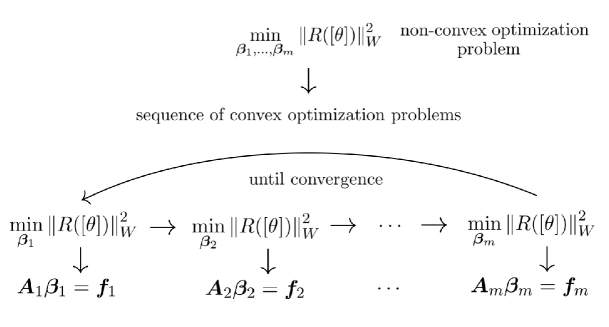
Figure 8: Sketch of the alternating least squares (ALS) algorithm for the minimization of the functional residual $R([\theta])$. Convergence analysis of ALS be found in [55, 19, 191, 219].

The Euler-Lagrange equations associated with (205) are in the form

$$\bm{A}_{j}\bm{\beta}_{j}=\bm{f}_{j}\qquad j=1,...,m,$$ (206)

where

$$\bm{A}_{j}=\left[\begin{array}[]{cccc}A^{11}_{j11}\cdots A^{11}_{j1Q}&A^{12}_{j11}\cdots A^{12}_{j1Q}&\cdots&A^{1r}_{j11}\cdots A^{1r}_{j1Q}\\ \vdots&\vdots&\vdots&\vdots\\ A^{11}_{jQ1}\cdots A^{11}_{jQQ}&A^{12}_{jQ1}\cdots A^{12}_{jQQ}&\cdots&A^{1r}_{jQ1}\cdots A^{1r}_{jQQ}\\ \vdots&\vdots&\vdots&\vdots\\ A^{r1}_{j11}\cdots A^{r1}_{j1Q}&A^{r2}_{j11}\cdots A^{r2}_{j1Q}&\cdots&A^{rr}_{j11}\cdots A^{rr}_{j1Q}\\ \vdots&\vdots&\vdots&\vdots\\ A^{r1}_{jQ1}\cdots A^{r1}_{jQQ}&A^{r2}_{jQ1}\cdots A^{r2}_{jQQ}&\cdots&A^{rr}_{jQ1}\cdots A^{rr}_{jQQ}\end{array}\right],\qquad\bm{f}_{j}=\left[\begin{array}[]{c}f_{j1}^{1}\\ \vdots\\ f_{jQ}^{1}\\ \vdots\\ f_{j1}^{r}\\ \vdots\\ f_{jQ}^{r}\\ \end{array}\right],$$ (207)

and

$$A^{ln}_{jhs}=\int\mathcal{D}[\theta]W([\theta])\phi_{h}((\theta,\varphi_{j}))\phi_{s}((\theta,\varphi_{j}))\prod_{\begin{subarray}{c}k=1\\ k\neq j\end{subarray}}^{m}G_{k}^{l}((\theta,\varphi_{k}))G_{k}^{n}((\theta,\varphi_{k})),$$ (208)

$$f_{jh}^{n}=\int\mathcal{D}[\theta]W([\theta])F([\theta])\phi_{h}((\theta,\varphi_{j}))\prod_{\begin{subarray}{c}k=1\\ k\neq j\end{subarray}}^{m}G_{k}^{n}((\theta,\varphi_{k})).$$ (209)

The matrices $\bm{A}_{j}$ are symmetric, positive definite and of size $rQ\times rQ$. Also, the functional integrals defining the matrix entries can be simplified and eventually computed by using techniques for high-dimensional integration, such as the quasi-Monte Carlo method [40]. Indeed, if we restrict the residual (200) to the finite-dimensional function space $D_{m}=\textrm{span}\{\varphi_{1},...,\varphi_{m}\}$ (Section 3.1), and assume that $F([\theta])$ restricted to $D_{m}$ is compactly supported within the hypercube $[-b,b]^{m}$, then $A^{ln}_{jhp}$ and $f_{jh}^{n}$ can be written in the form

$$A^{ln}_{jhs}=\int_{-b}^{b}\phi_{h}(a_{j})\phi_{s}(a_{j})da_{j}\prod_{\begin{subarray}{c}k=1\\ k\neq j\end{subarray}}^{m}\int_{-b}^{b}G_{k}^{l}(a_{k})G_{k}^{n}(a_{k})da_{k},$$ (210)

$$f_{jh}^{n}=\int_{-b}^{b}\cdots\int_{-b}^{b}f(a_{1},...,a_{m})\phi_{h}(a_{j})\prod_{\begin{subarray}{c}k=1\\ k\neq j\end{subarray}}^{m}G_{k}^{n}(a_{k})da_{1}\cdots da_{m},$$ (211)

provided we select the integration measure $W([\theta])$ appropriately (see Appendix B).

Remark: Minimizing the residual (200) with respect to $\beta_{hj}^{n}$ is equivalent to imposing orthogonality relative to the space spanned by the functionals

$$\phi_{h}((\theta,\phi_{j}))\prod^{m}_{\begin{subarray}{c}k=1\\ k\neq j\end{subarray}}G^{n}_{k}((\theta,\varphi_{k}))$$ (212)

To show this in a simple and intuitive way, consider the following example in just two dimensions. Let $f(a_{1},a_{2})$ be a regular function defined on the unit square $[0,1]^{2}$. We look for a canonical tensor decomposition of $f(a_{1},a_{2})$ in the form

$$f(a_{1},a_{2})=\sum_{j=1}^{r}G^{j}_{1}(a_{1})G^{j}_{2}(a_{2}),\quad\textrm{where}\quad G^{j}_{k}(a_{k})=\sum_{p=1}^{P}\beta^{j}_{kp}\phi_{p}(a_{k}).$$ (213)

To determine $\beta^{j}_{kp}$ we first define the residual,

$$R(a_{1},a_{2})=f(a_{1},a_{2})-\sum_{j=1}^{r}G^{j}_{1}(a_{1})G^{j}_{2}(a_{2})$$ (214)

and then minimize its weighed norm

$$\left\|R\right\|^{2}_{w}=\int_{0}^{1}\int_{0}^{1}R(a_{1},a_{2})^{2}w(a_{1},a_{2})da_{1}da_{2}$$ (215)

relative to independent variations of $\beta^{j}_{1p}$ and $\beta^{j}_{2p}$. This yields

$$\begin{array}[]{ll}\displaystyle\int_{0}^{1}\int_{0}^{1}w(a_{1},a_{2})R(a_{1},a_{2})\phi_{p}(a_{1})G_{2}^{j}(a_{2})da_{1}da_{2}=0&\quad\textrm{linear system for $\beta^{j}_{1p}$},\vspace{0.2cm}\\ \displaystyle\int_{0}^{1}\int_{0}^{1}w(a_{1},a_{2})R(a_{1},a_{2})G_{1}^{j}(a_{1})\phi_{p}(a_{2})da_{1}da_{2}=0&\quad\textrm{linear system for $\beta^{j}_{2p}$.}\end{array}$$ (216)

Thus, minimizing the residual with respect to independent variations of $\beta^{j}_{1p}$ and $\beta^{j}_{2p}$ is equivalent impose Galerkin orthogonality relative to a space spanned by the basis functions $\phi_{p}(a_{1})G_{2}^{j}(a_{2})$ and $G_{1}^{j}(a_{1})\phi_{p}(a_{2})$, respectively.

Convergence of the ALS Algorithm

The ALS algorithm we just described is an alternating optimization scheme, i.e., a nonlinear block Gauss–Seidel method ([167], §7.4). There is a well–developed local convergence theory for this type of method (see [167, 19]). In particular, it can be shown that ALS is locally equivalent to the linear block Gauss–Seidel iteration applied to the Hessian matrix. This implies that ALS is linearly convergent in the iteration number [219], provided that the Hessian of the residual is positive definite (except on a trivial null space associated with the scaling non-uniqueness of the canonical tensor decomposition). The last assumption may not be always satisfied. Therefore, convergence of the ALS algorithm cannot be granted in general. Another potential issue of the ALS algorithm is the poor conditioning of the matrices $\bm{A}_{j}$ in (206), which can addressed by regularization [188, 12]. The canonical tensor decomposition (187) in $m$ dimensions has relatively small memory requirements. In fact, the number of degrees of freedom that we need to store is $r\times m\times Q$, where $r$ is the separation rank, and $Q$ is the number of degrees of freedom employed in each tensor component $G_{k}^{l}(a_{k})$ (188). Despite the relatively low-memory requirements, it is often desirable to employ scalable parallel versions the ALS algorithm [100] to compute the canonical tensor expansion (187).

3.3.2 Tucker Decomposition

The Tucker decomposition of the cylindrical functional (180) is a series expansion in the form

$$f(a_{1},...,a_{m})=\sum_{l_{1}=1}^{r_{1}}\cdots\sum_{l_{m}=1}^{r_{m}}C_{l_{1}\cdots l_{m}}T^{l_{1}}_{1}(a_{1})\cdots T^{l_{m}}_{m}(a_{m}),$$ (217)

where $C_{l_{1}...l_{m}}$ is a $r_{1}\times\cdots\times r_{m}$ real- or complex-valued tensor – often referred to as core tensor [113] – and $T^{l_{m}}_{m}(a_{m})$ are unknown functions. Tucker decomposition is known as high-order Schmidt decomposition in the context of quantum mechanics [27]. It is important to emphasize such decomposition is, in general, are not unique. As pointed out by Kolda and Bader in [113], this freedom opens the possibility to choosing transformations that simplify the core structure in some way so that most of the elements of the core tensor $C_{l_{1}\cdots l_{m}}$ are zero, thereby eliminating interactions between corresponding components. Diagonalization of the core is, in general, impossible [171], but it is possible to try to make as many elements either zero or as small as possible (see, e.g., [27] or [147]). For general tensors we have that the multilinear rank $r=r_{j}$ ($j=1,...,m$) is upper semi-continuous, i.e., the Tucker expansion is closed. Several efficient algorithms are currently available to compute the series expansion (217). For instance, Lathauwer et al. proposed in [118] a high-order singular value decomposition method to determine the components $T_{k}^{l_{k}}$ and the core tensor $C_{l_{1}\cdots l_{m}}$ in a discrete setting. Such algorithm is simple, robust and it yields quasi-optimal low-rank approximations.

To illustrate the procedure to compute the Tucker decomposition let us first assume that the basis functions $T_{k}^{l_{k}}(a_{k})$ in (217) are orthonormal and known. In this case, the expansion (217) is simply a tensor product representation of a multivariate function relative to the basis $T_{k}^{l_{k}}$. The core tensor $C_{l_{1}\cdots l_{m}}$ can be immediately obtained by projecting $f(a_{1},...,a_{m})$ onto the basis $T_{k}^{l_{k}}(a_{k})$, i.e.,

$$C_{l_{1}\cdots l_{m}}=\int f(a_{1}([\theta]),...,a_{m}([\theta]))T_{1}^{l_{1}}(a_{1}([\theta]))\cdots T_{m}^{l_{m}}(a_{m}([\theta]))W([\theta])\mathcal{D}([\theta]).$$ (219)

Evaluating the functional integral in $D_{m}=\textrm{span}\{\varphi_{1},...,\varphi_{m}\}$ and rescaling the integration measure $W([\theta])$ properly (see Appendix B) allows us to rewrite (219)

$$C_{l_{1}\cdots l_{m}}=\int_{-b}^{b}\cdots\int_{-b}^{b}f(a_{1},...,a_{m})T_{1}^{l_{1}}(a_{1})\cdots T_{m}^{l_{m}}(x_{m})da_{1}\cdots da_{m},$$ (220)

where we assumed $f$ to be compactly supported in $[-b,b]^{m}$. Next, suppose that each function $T_{k}^{l_{k}}(a_{k})$ is a linear combination of $Q$ orthonormal basis functions $\phi_{j}$, i.e.,

$$T_{k}^{l_{k}}(a_{k})=\sum_{s=1}^{Q}\alpha_{sk}^{l_{k}}\phi_{s}(a_{k})\qquad\textrm{(fixed $k$).}$$ (221)

If $\phi_{s}$ is a cardinal basis associated with a set of interpolation nodes along $a_{k}$, then the matrix $\alpha_{sk}^{l_{k}}$ represents the set of functions $T_{k}^{l_{k}}(a_{k})$ for fixed $k$. We can sort arrange the matrix $\alpha_{sk}^{l_{k}}$ in a way where the $l_{k}$-column represents the value of $T_{k}^{l}(a_{k})$ at $Q$ collocation nodes along $a_{k}$. This yields the matrix with entries $[T_{k}]_{il}$ ($i=1,...,Q$). If we evaluate the multivariate field $f(a_{1},..,a_{m})$ at the same collocation nodes we employed to construct the interpolants of $T_{k}^{l_{k}}$, then we can rewrite (217) in a full tensor notation as

$$f_{i_{1}\cdots i_{m}}=\sum_{l_{1}=1}^{r_{1}}\cdots\sum_{l_{m}=1}^{r_{m}}C_{l_{1},...,l_{m}}[T_{1}]_{i_{1}l_{1}}\cdots[T_{m}]_{i_{m}l_{m}},$$ (222)

where $i_{j}=1,...,Q$ are indices identifying the interpolation node along the axis $a_{j}$.

Remark: The expansion (222) is a “matricization” of continuum series (217) obtained by representing each basis element in terms of collocation nodes. Clearly, we can also set up a matricization of (217) based on Galerkin projection. To this end, it is sufficient to project both the left and the right hand sides of (217) onto the orthonormal basis elements $\phi_{i_{1}}(a_{1})\phi_{i_{2}}(a_{2})\cdots\phi_{i_{m}}(a_{m})$ to obtain an expression in the form (222). The meaning of $f_{i_{1}\cdots i_{n}}$ in the case is the Fourier coefficients of the projection, i.e.,

$$f_{i_{1}\cdots i_{n}}=\int_{-b}^{b}\cdots\int_{-b}^{b}f(a_{1},...,a_{m})\phi_{i_{1}}(a_{1})\cdots\phi_{i_{m}}(a_{m})dx_{1}\cdots dx_{m}.$$ (223)

Thus, (222) represents a multivariate expansion of Fourier coefficients in a Tucker tensor format. In such finite-dimensional setting, we basically transformed the problem of decomposing a multivariate function to a multi-linear algebra problem. It is immediate to see that the discrete Tucker format a two-dimensional function $f(a_{1},a_{2})$ is

$$f_{i_{1}i_{2}}=\sum_{l_{1}=1}^{r_{1}}\sum_{l_{2}=1}^{r_{2}}C_{l_{1}l_{2}}[T_{1}]_{i_{1}l_{1}}[T_{2}]_{i_{2}l_{2}},$$ (224)

We can obviously diagonalize the core tensor by using singular value decomposition.

A drawback of the Tucker decomposition is the storage requirement of the core tensor $C_{l_{1}\cdots l_{m}}$, which is $O(r^{m})$. Such problem can be mitigated by attempting to make zero as many entries of $C_{l_{1}\cdots l_{m}}$ as possible through suitable linear transformations. Another option is to introduce further separability properties of the core tensor. This yields a multitude of possible expansions, including hierarchical Tucker [75, 8] and Tucker tensor train [159, 191]. All these series expansions can be conveniently visualized by suitable graphs, and as such they fall within the setting of tensor-networks.

3.3.3 Hierarchical Tucker Decomposition

We have seen that the canonical tensor decomposition of a nonlinear functional has a relatively small number of degrees of freedom, but its computation is not straightforward. The most reliable algorithms are based on regularized optimization and randomized methods (see [188, 12] for recent results), which often yield different series expansions for different initial conditions. On the other hand, we have seen the that high-order Schmidt decomposition suffers from the curse of dimensionality (dimension of the core tensor), but it is straightforward to compute by nearly optimal and robust techniques such as high-order singular value decomposition [118]. The hierarchical Tucker format was introduced by Hackbush and Kühn in [79] (see also [78, 75]) to mitigate the dimensionality problem in the core-tensor of the classical high-order Schmidt decomposition. The key idea is to perform a sequence of classical bi-variate Schmidt decompositions until the approximation problem is reduced to a product of one-dimensional functions. To illustrate the method is a simple way, consider the following cylindrical functional

$$f(a_{1},a_{2},a_{3})=\sum_{i,j=1}^{r}A^{\{1\}}_{ij}T^{\{1\}}_{i}(a_{1})T^{\{2,3\}}_{j}(a_{2},a_{3}),\qquad a_{j}=(\theta,\varphi_{j}).$$ (225)

The matrix representation of $f(a_{1},a_{2},a_{3})$ (either Galerkin or collocation form) relative to the given bases $T^{\{1\}}_{i}$ and $T^{\{2,3\}}_{j}$ is $A_{ij}^{\{1\}}$, i.e., it has two indices. We decompose $T^{\{2,3\}}_{j}$ further by another Schmidt expansion

$$T^{\{2,3\}}_{j}(a_{2},a_{3})=\sum_{l,n=1}^{r}A^{\{2\}}_{jln}T^{\{2\}}_{l}(a_{2})T^{\{3\}}_{n}(a_{3}),$$ (226)

to obtain

$$f(a_{1},a_{2},a_{3})=\sum_{i,j,l,n=1}^{r}A^{\{2\}}_{jln}A^{\{1\}}_{ij}T^{\{1\}}_{i}(x_{1})T^{\{2\}}_{l}(a_{2})T^{\{3\}}_{n}(a_{3}).$$ (227)

The procedure just described is at the basis of the hierarchical Tucker decomposition and it yields an expansion in the form (217), where the core tensor is factored as a product of at most three-dimensional tensors. To show this in a higher-dimensional case, consider the six-dimensional cylindrical functional $f(a_{1},...,a_{6})$. By performing a sequence of Hilbert-Schmidt factorizations, while keeping the separation rank $r$ constant in each factorization, we obtain

$$f(a_{1},...,a_{6})= \sum_{i_{7},i_{8}=1}^{r}A^{\{1\}}_{i_{7}i_{8}}T^{\{1,2,3\}}_{i_{7}}(a_{1},a_{2},a_{3})T^{\{4,5,6\}}_{i_{8}}(a_{4},a_{5},a_{6}),$$

$$= \sum_{i_{7},i_{8}=1}^{r}A^{\{1\}}_{i_{7}i_{8}}\sum_{i_{1},i_{9}=1}^{r}A^{\{2\}}_{i_{7}i_{1}i_{9}}T^{\{1\}}_{i_{1}}(a_{1})T^{\{2,3\}}_{i_{9}}(a_{2},a_{3})\sum_{i_{4},i_{10}=1}^{r}A^{\{3\}}_{i_{8}i_{4}i_{10}}T^{\{4\}}_{i_{4}}(a_{4})T^{\{5,6\}}_{i_{10}}(a_{5},a_{6}),$$

$$=\sum_{i_{1},\cdots,i_{6}=1}^{r}C_{i_{1}\cdots i_{6}}T^{\{1\}}_{i_{1}}(a_{1})T^{\{2\}}_{i_{2}}(a_{2})T^{\{3\}}_{i_{3}}(a_{3})T^{\{4\}}_{i_{4}}(a_{4})T^{\{5\}}_{i_{5}}(a_{5})T^{\{6\}}_{i_{6}}(a_{6}),$$ (228)

where the $6$-dimensional core tensor is explicitly given

$$C_{i_{1}\cdots i_{6}}=\sum_{i_{7},i_{8}=1}^{r}A^{\{1\}}_{i_{7}i_{8}}\sum_{i_{9}=1}^{r}A^{\{2\}}_{i_{7}i_{1}i_{9}}A^{\{4\}}_{i_{9}i_{2}i_{3}}\sum_{i_{10}=1}^{r}A^{\{3\}}_{i_{8}i_{4}i_{10}}A^{\{5\}}_{i_{10}i_{5}i_{6}}.$$ (229)

Note that such kernel has a recursive structure and it is factored as a product of at most three-dimensional matrices. Parallel algorithms to perform basic operations on hierarchical Tucker expansions such as addition, multiplication, and rank reduction were recently proposed in [77, 56]. Also, an optimization framework that leverages on the on recursive subspace factorizations of Hierarchical Tucker expansions was developed in [206].

3.3.4 Tensor Train Decomposition

If we single-out one variable at a time and perform a sequential Schmidt decomposition of the remaining variables we obtain the so-called tensor-train decomposition [168, 191]. Tensor train decomposition is a subcase case of hierarchical Tucker decomposition. For example, the tensor train decomposition of the four-dimensional cylindrical functional $f(a_{1},...,a_{4})$ reads

$$f(a_{1},...,a_{4})= \sum_{i1,i_{2}=1}^{r}A^{\{1\}}_{i_{1}i_{2}}T^{\{1\}}_{i_{1}}(a_{1})T^{\{2,3,4\}}_{i_{2}}(a_{2},a_{3},a_{4}),$$

$$= \sum_{i_{1},i_{2}=1}^{r}A^{\{1\}}_{i_{1}i_{2}}T^{\{1\}}_{i_{1}}(a_{1})\sum_{i_{3},i_{4}=1}^{r}A^{\{2\}}_{i_{2}i_{3}i_{4}}T^{\{2\}}_{i_{3}}(a_{2})T^{\{3,4\}}_{i_{4}}(a_{3},a_{4}),$$

$$= \sum_{i_{1},...,i_{4}=1}^{r}A^{\{1\}}_{i_{1}i_{2}}A^{\{2\}}_{i_{2}i_{3}i_{4}}T^{\{1\}}_{i_{1}}(a_{1})T^{\{2\}}_{i_{3}}(a_{2})\sum_{i_{5},i_{6}}^{r}A^{\{3\}}_{i_{4}i_{5}i_{6}}T^{\{3\}}_{i_{5}}(a_{3})T^{\{4\}}_{i_{6}}(a_{4}),$$

$$= \sum_{i_{1},...,i_{6}=1}^{r}A^{\{1\}}_{i_{1}i_{2}}A^{\{2\}}_{i_{2}i_{3}i_{4}}A^{\{3\}}_{i_{4}i_{5}i_{6}}T^{\{1\}}_{i_{1}}(a_{1})T^{\{2\}}_{i_{3}}(a_{2})T^{\{3\}}_{i_{5}}(a_{3})T^{\{4\}}_{i_{6}}(a_{4}).$$ (230)

Tensor train and hierarchical Tucker expansions can be conveniently visualized by graphs.

3.3.5 Tensor Networks

During the last decades, the field of Tensor Networks has undergone an explosion of results in several different directions, e.g., in the study of quantum many-body systems, and more generally in multivariate functional approximation. Tensor networks can be conveniently represented by undirected graphs. To this end, we adopt the following standard convention:

• a node in a graph represents a tensor in as many variables as the number of the edges connected to it;

• connecting two tensors by an edge represents a tensor contraction over the index associated to certain variable.

In this way, a three-dimensional Tucker format is represented by one node with three edges emanating from it. If we connect two of such tensors with one edge, then we obtain a tensor in four variables. In particular, the connection operation here results in a Tucker format with the core tensor represented by a product of two three-dimensional tensors in which we contract one index (see Figure 9).

Tucker Format                                                     Tensor Network

                                    

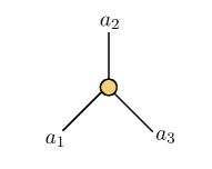
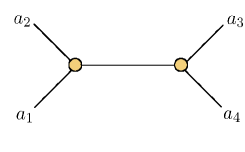
$\displaystyle\sum_{i_{1},i_{2},i_{3}=1}^{r}A_{i_{1}i_{2}i_{3}}T^{\{1\}}_{i_{1}}(a_{1})T^{\{2\}}_{i_{2}}(a_{2})T^{\{3\}}_{i_{3}}(a_{3})$              $\displaystyle\sum_{i_{1},...,i_{4}=1}^{r}\left(\sum_{j=1}^{r}A^{\{1\}}_{i_{1}i_{2}j}A^{\{2\}}_{ji_{3}i_{4}}\right)T^{\{1\}}_{i_{1}}(a_{1})T^{\{2\}}_{i_{2}}(a_{2})T^{\{3\}}_{i_{3}}(a_{3})T^{\{4\}}_{i_{4}}(a_{4})$

Figure 9: Examples of tensor networks representing a cylindrical functional in three and four variables.

The graph representation of the hierarchical Tucker and tensor train decomposition is shown in Figure 10.

Hierarchical Tucker                                     Tensor Train

         

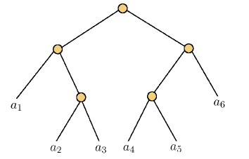
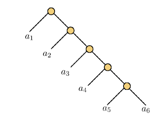
Figure 10: Graph representation of the Hierarchical Tucker (HT) and tensor train (TT) decomposition of a six-dimensional cylindrical functional.

A more general tensor network representation of a cylindrical functional in five variables is shown in Figure 11.

     Tensor Network                           Equivalent Tucker Format

                 

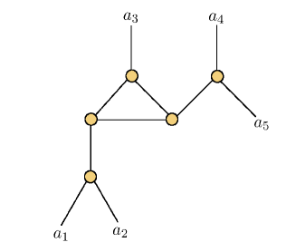
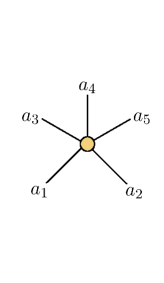
Figure 11: Tensor network representation of a five-dimensional cylindrical functional. After reduction (elimination of the cycle and connection of nodes), it is easy to see the graph is equivalent to the graph corresponding to a Tucker format of dimension five (right). The core tensor of such Tucker format is expressed as products and contractions of at most three-dimensional tensors.

Note that each node is connected with at most three edges (coordination number equal to three) as we employed a Schmidt decomposition to represent each function with more than one variable. Clearly, the graph can be reduced to one node with five leaves (i.e. a Tucker series) by eliminating the cycle and clustering all nodes that are connected by edges [114] . The graph can be therefore reduced to a node with five leaves – i.e. a Tucker series, with a particular structure of the core tensor. At this point the graph is irreducible (one node with five leaves). Efficient algorithms that implement basic operations between tensors, such as addition, orthogonalization, rank reduction, scalar products, multiplication, and linear transformations are discussed in [114, 56, 76, 159, 113].

3.4 Generalized Lagrangian Interpolation

We have seen that the classical Lagrange interpolation problem for multivariate functions can be generalized to functionals in Hilbert or Banach spaces, i.e., objects depending on an infinite number of variables. Given a real-valued continuous functional

$$F:D(F)\rightarrow\mathbb{R},$$ (231)

and a set of elements $\{\theta_{1}(x),...,\theta_{n}(x)\}$ in $D(F)$, the Lagrangian interpolant of $F$ is a continuous functional

$$\Pi:D(F)\rightarrow\mathbb{R},$$ (232)

such that

$$\Pi([\theta_{i}])=F([\theta_{i}]).$$ (233)

A simple representation of $\Pi([\theta])$ can be given in terms of cardinal basis functionals $g_{i}:D(F)\rightarrow\mathbb{R}$ as

$$\Pi([\theta])=\sum_{i=1}^{n}F([\theta_{i}])g_{i}([\theta]),\quad\textrm{where}\quad g_{i}([\theta_{j}])=\delta_{ij}.$$ (234)

Similarly to classical Lagrange interpolation for functions from $\mathbb{R}^{n}$ to $\mathbb{R}^{m}$, we have a great freedom in selecting $g_{i}([\theta])$. We have already seen, for example, Porter’s and Prenter’s cardinal bases defined in equation (113) and equation (150), respectively. Now, let

$$\kappa:D(F)\times D(F)\rightarrow\mathbb{R}$$ (235)

be any continuous (not necessarily symmetric) functional subject to the sole requirement that

$$\kappa([\theta],[\eta])=0\quad\Leftrightarrow\quad\theta(x)=\eta(x).$$ (236)

Examples of such functional are

$$\kappa_{1}([\theta],[\eta]) =\left\|\theta(x)-\eta(x)\right\|^{p},\qquad p>0$$ (237)

$$\kappa_{2}([\theta],[\eta]) =\left\|\theta(x)-\eta(x)\right\|+\left\|\theta(x)\right\|-\left\|\eta(x)\right\|.$$ (238)

$$\kappa_{3}([\theta],[\eta]) =1-\exp\left(-\left\|\theta(x)-\eta(x)\right\|^{2}\right).$$ (239)

By using $\kappa([\theta],[\eta])$ we define the following cardinal basis associated with the interpolation nodes $\{\theta_{1}(x),...,\theta_{n}(x)\}$ in $D(F)$ (see [30], Ch. 10)

$$g_{i}([\theta])=\prod_{\begin{subarray}{c}j=1\\ j\neq i\end{subarray}}^{n}\frac{\kappa([\theta],[\theta_{j}])}{\kappa([\theta_{i}],[\theta_{j}])}\qquad i=1,...,n.$$ (240)

A substitution of (240) into (234) yields a Lagrangian functional interpolant that depends on the choice of $\kappa([\theta],[\eta])$. An advantage of such interpolant over Porter’s interpolant is that the basis functionals (240) are given analytically and do not require any computation such as the inversion (and storage) of the $H$-matrix (111). On the other hand, we have no guarantee that (240) have good approximation properties away from the interpolation nodes. The Lagrange interpolation formula (234)-(240) can be written in a barycentric form. To this end, we first rewrite the numerator of (240) as $\Omega([\theta])/\kappa([\theta],[\theta_{i}])$, where

$$\Omega([\theta])=\prod_{i=k}^{n}\kappa([\theta],[\theta_{k}]).$$ (241)

Then define the barycentric weights as

$$w_{i}=\prod_{\begin{subarray}{c}j=1\\ j\neq i\end{subarray}}^{n}\frac{1}{\kappa([\theta_{i}],[\theta_{j}])}.$$ (242)

Clearly,

$$g_{i}([\theta])=\Omega([\theta])\frac{w_{i}}{\kappa([\theta],[\theta_{i}])}.$$ (243)

Substituting this into (234) and applying it to the constant functional $F([\theta])=1$ yields

$$\Omega([\theta])=\frac{1}{\displaystyle\sum_{i=1}^{n}\frac{w_{i}}{\kappa([\theta],[\theta_{i}])}}.$$ (244)

Therefore, we obtain the interpolant

$$\Pi([\theta])=\left(\sum_{i=1}^{n}\frac{w_{i}}{\kappa([\theta],[\theta_{i}])}\right)^{-1}\sum_{i=1}^{n}\frac{w_{i}F([\theta_{i}])}{\kappa([\theta],[\theta_{i}]).}$$ (245)

This expression can be evaluated in $\mathcal{O}(n)$ operations, provided we have available $w_{i}$, which needs $\mathcal{O}(n^{2})$ operations. What about updating? Adding a new interpolation node $\theta_{n+1}$ entails two calculations: 1) divide each $w_{j}$ by $\kappa([\theta_{j}],[\theta_{n+1}])$ and 2) compute $w_{n+1}$ using the formula (242).

Remark: The interpolation processes defined by (234) and (240) has a variation known as Shepard’s method [60, 121]. Such method was studied by Allasia and Bracco [4] for functional interpolation in Banach spaces and it relies on the cardinal functionals

$$g_{i}([\theta])=\frac{1}{\displaystyle 1+\sum_{\begin{subarray}{c}k=1\\ k\neq i\end{subarray}}^{n}\frac{{\kappa}([\theta],[\theta_{i}])}{{\kappa}([\theta],[\theta_{k}])}},\qquad i=1,...,n.$$ (246)

The kernel ${\kappa}([\theta],[\eta])$ here satisfies (236) and the additional positivity requirement

$${\kappa}([\theta],[\eta])>0\qquad\textrm{if}\qquad\theta(x)\neq\eta(x).$$ (247)

This implies that the basis functionals (246) have the following properties

$$0\leq g_{i}([\theta])\leq 1\quad\forall\theta\qquad g_{i}([\theta_{j}])=\delta_{ij}.$$ (248)

One unfortunate consequence of these conditions is that the functional derivative of $g_{i}([\theta])$ (if it exists) is identically zero at all nodes $\theta_{j}$. In fact, $g_{i}([\theta])$ is always positive, it has a maximum (equal to 1) at $\theta_{i}$ and many minima (equal to 0) at all other nodes. This yields functional differentiation matrices (120) that are identically zero. Functional Lagrangian interpolation can also be defined in terms of radial basis functionals $\kappa(\left\|\theta-\theta_{j}\right\|)$, for suitable choices of $\kappa$. In this cases, the cardinal basis $g_{i}([\theta])$ can be obtained by standard techniques such as the ratio of two Vandermonde determinants. Interpolation using radial basis functionals can converge towards polynomial functional interpolants if we take increasingly flat radial bases (see, e.g., [202, 47, 208]).

The Lagrangian interpolation process defined by (234), (236) and (240) can be generalized further by considering a family of continuous functionals

$$\kappa_{i}:D(F)\times D(F)\rightarrow\mathbb{R},\qquad i=1,...,n$$ (249)

as many as the number of interpolation nodes, satisfying $\kappa_{i}([\theta],[\theta_{j}])\neq 0$ for $i\neq j$, $\kappa_{i}([\theta],[\theta_{i}])=0$ and $\kappa_{i}([\theta],[\theta])=0$. The cardinal basis corresponding to $\{\kappa_{1},...,\kappa_{n}\}$ is

$$g_{i}([\theta])=\prod_{\begin{subarray}{c}j=1\\ j\neq i\end{subarray}}^{n}\frac{\kappa_{i}([\theta],[\theta_{j}])}{\kappa_{i}([\theta_{i}],[\theta_{j}])}.$$ (250)

In particular, the choice

$$\kappa_{i}([\theta],[\eta])=(\theta-\eta,\theta_{i}-\eta)$$ (251)

yields Prenter’s cardinal basis (150). It fact,

$$\kappa_{i}([\theta],[\theta_{j}]) =(\theta-\theta_{j},\theta_{i}-\theta_{j}),$$ (252)

$$\kappa_{i}([\theta_{i}],[\theta_{j}]) =\left\|\theta_{i}-\theta_{j}\right\|^{2},$$ (253)

$$\kappa_{i}([\theta],[\theta_{i}]) =0.$$ (254)

Another generalization of the Lagrange interpolation process can be obtained along the lines of Porter’s functional interpolants. To this end, let $\kappa([\theta],[\eta])$ be any symmetric functional such that the matrix

$$H_{ij}=\kappa([\theta_{i}],[\theta_{j}])$$ (255)

is invertible for every set of distinct nodes $\{\theta_{j}(x)\}$. Then the functional

$$\Phi_{n}([\theta])=\sum_{k=1}^{m}F(\theta_{k})\underbrace{\sum_{j=1}^{m}\kappa([\theta_{k}],[\theta_{j}])^{-1}\kappa([\theta],[\theta_{j}])}_{g_{k}([\theta])},$$ (256)

where $\kappa([\theta_{k}],[\theta_{j}])^{-1}$ denotes the inverse matrix of (255), interpolates $F([\theta])$ at $\theta_{k}(x)$ ($k=1,...,m$). The question of how to select the symmetric functional $\kappa$ depends on the requirements we impose on the behavior of the functional interpolant away from the interpolation nodes. In particular, the choice

$$\kappa([\theta],[\eta])=\sum_{p=0}^{n}(\theta,\eta)^{p}$$ (257)

yields Porter’s interpolants, i.e., polynomial functionals of order $n$ with minimal norm.

3.4.1 Optimal Interpolation Nodes

In this Section we briefly address the question of how to select the interpolation nodes in the function space $D(F)$ in such a way that the corresponding functional interpolant, e.g., the Porter’s one (112)-(113), exhibits good approximation properties.

Adaptive Leja Sequences

An effective approach to select sub-optimal interpolation nodes relies on adaptive Leja sequences [151, 23]. In this setting, given the set of nodes $\{\theta_{1}(x),...,\theta_{n}(x)\}$ in $D(F)$, the problem is to find a new node $\theta^{*}(x)$ satisfying the maximization principle

$$\operatorname*{arg\,max}_{\theta^{*}(x)\in D(F)}\left|\det(V)\right|$$ (258)

where $V$ is a Vandermonde-like operator (infinite-dimensional matrix) (see [23, 151, 153, 135] for further details). This results in the so-called Leja construction of the test function $\theta^{*}(x)$, a greedy version of the well-known Fekete construction involving nonlinear optimization. There are also non-determinant versions of multivariate Leja interpolation nodes, which are related to potential theory [128, 93]. In this setting, given a symmetric functional $\kappa([\theta(x)],[\eta(x)])$ one can construct a greedy $\kappa$-energy sequence in which $\theta^{*}(x)$ is chosen to satisfy

$$\sum_{i=1}^{n}\kappa([\theta^{*}(x)],[\theta_{i}(x)])=\operatorname*{arg\,min}_{\theta^{*}\in D(F)}\sum_{i=1}^{n}\kappa([\theta^{*}(x)],[\theta_{i}(x)]),$$ (259)

assuming $\{\theta_{1}(x),...,\theta_{n}(x)\}$ are available. The element $\theta^{*}(x)$ obtained in this way is not unique. Also, depending on the choice of the kernel function $\kappa([\theta(x)],[\eta(x)])$, we can have different sets of nodes. A relevant kernel for the $\kappa$-energy sequence is the so-called Riesz $p$-kernel

$$\kappa_{p}([\theta(x)],[\eta(x)])=\begin{cases}\displaystyle\frac{1}{\left\|\theta(x)-\eta(x)\right\|^{p}}&\textrm{if $p>0$}\\ \displaystyle-\ln(\left\|\theta(x)-\eta(x)\right\|)&\textrm{if $p=0$}\\ \end{cases}$$ (260)

Such kernel avoids placing points too close to each other (the potential $\kappa_{p}$ is rather large in such regions), while decreasing monotonically at larger distances. The asymptotic behavior of greedy $\kappa$-energy sequences has been studied theoretically by López-García and Saff [128], in a finite-dimensional setting.

Minimization of Lebesgue Functionals

Another approach to determine sub-optimal nodes in the function space $D(F)$ relies on greedy algorithms minimizing Lebesgue-like functionals. This problem has been recently addressed in a finite-dimensional setting by Narayan and Xiu [153, 152], Maday et al. [131, 132] and Van Barel et. al [10]. The basic idea is simple and can be generalized to the infinite-dimensional case. Suppose we have available $\{\theta_{1}(x)$, …, $\theta_{n}(x)\}$. We look for a new node $\theta^{*}(x)$ maximizing a suitable objective functional, e.g., related to the well-known Lebesgue function in finite-dimensional interpolation problems. In particular, following the weighed approach of Narayan and Xiu [153], we can look for a new node $\theta^{*}(x)$ satisfying the following (greedy) optimization problem

$$\operatorname*{arg\,max}_{\theta^{*}\in D(F)}\chi([\theta^{*}]),\qquad\chi([\theta])=W([\theta])^{2}\sum_{k=1}^{n}\frac{g_{k}([\theta])^{2}}{W([\theta_{k}])^{2}},$$ (261)

where $W([\theta])$ is a positive functional and $g_{i}([\theta])$ is a cardinal basis. Other choices of $\chi([\theta])$ yield different sets of nodes. For example,

$$\chi([\theta])=W([\theta])\sum_{k=1}^{n}\frac{g_{i}([\theta])^{2}}{W([\theta_{k}])}$$ (262)

yields an infinite-dimensional extension of the Fejér points. The sequence of nodes $\theta_{i}(x)$ we obtain in this way strongly depends on the initial set of nodes, on the weight $W([\theta])$ and on the cardinal basis $\{g_{i}(\left[\theta\right])\}$. Finding the maximum of (261) involves computing the solution to an optimization problem in infinite dimensions [14]. A necessary condition for a stationary point of (261) is

$$\frac{\delta\chi([\theta])}{\delta\theta(x)}=0.$$ (263)

Example 1: The Euler-Lagrange equation (263) can be written down explicitly, e.g., for Porter’s interpolants. To this end, simply substitute (113) in (262) and set $W=1$ to obtain

$$\chi([\theta])=\sum_{k=1}^{n}\sum_{j,z=1}^{m}H_{jk}^{-1}H_{zk}^{-1}\sum_{p,q=0}^{h}\left(\theta_{j},\theta\right)^{p}\left(\theta_{z},\theta\right)^{q}.$$ (264)

This allows us to write explicitly the conditions identifying stationary points of $\chi([\theta])$, e.g., in the function space

$$D_{N}=\left\{\theta(x)\in D(F)\,\left|\,\theta(x)=\sum_{k=1}^{N}a_{k}\varphi_{k}(x)\right.\right\}.$$ (265)

3.5 High-Dimensional Model Representation

The high-dimensional model representation (HDMR) [185, 126, 125, 26] of the cylindrical functional (177) is a series expansion in the form

$$f(a_{1},...,a_{m})=f_{0}+\sum_{k=1}^{m}f_{k}(a_{k})+\sum_{\begin{subarray}{c}k,j=1\\ k<j\end{subarray}}^{m}f_{kj}(a_{k},a_{j})+\cdots.$$ (266)

The functional $f_{0}$ is simply a constant. The functionals $f_{i}(a_{i})$, which we shall call first-order interaction terms, give us the overall effects of the variables $a_{i}=(\theta,\varphi_{i})$ in $f$ as if they were acting independently of the other variables. The functions $f_{ij}(a_{i},a_{j})$ represent the interaction effects of $a_{i}$ and $a_{j}$, and therefore they are usually called second-order interactions. Similarly, higher-order terms reflect the cooperative effects of an increasing number of variables. The interaction terms in the HDMR expansion can be easily computed if we assume that the domain of $f$ is compactly supported and included in the hypercube $[-b,b]^{m}$ (see Appendix B). By introducing the finite-dimensional integration measure $w(\bm{a})=w(a_{1},...,a_{m})$ and the vector notation $d\bm{a}_{-i}=da_{i-1}da_{i+1}\cdots da_{m}$, we have

$$f_{0} =\int_{[-b,b]^{m}}w(\bm{a})f(\bm{a})d\bm{a},$$ (267)

$$f_{i}(a_{i}) =\int_{[-b,b]^{m-1}}w(\bm{a})f(\bm{a})d\bm{a}_{-i}-f_{0},$$ (268)

$$f_{ij}(a_{i},a_{j}) =\int_{[-b,b]^{m-2}}w(\bm{a})f(\bm{a})d\bm{a}_{-ij}-f_{i}(a_{i})-f_{j}(a_{j})-f_{0},$$ (269)

$$\cdots.$$

This procedure generates, by construction, terms that are orthogonal in the weighted $L_{2}$ sense. The HDMR series (266) with components (267)-(269) is often called ANOVA-HDMR expansion. If we consider a Dirac delta measure $w(\bm{a})=\delta(a_{1}-c_{1})\cdots\delta(a_{m}-c_{m})$ with “anchor point” $\bm{c}=(c_{1},...,c_{m})$, then the HDMR series is called CUT-HDMR [39, 249]. There is also a random-sampling version of HDMR – namely the RS-HDMR [125] expansion – in which the high-dimensional integrals in (267)-(268) are computed by Monte-Carlo or quasi-Monte Carlo methods. The HDMR expansion (266) is usually truncated at some interaction order, and the interactions $f_{i}$, $f_{ij}$ are expanded relative to a certain basis. For example, the first-order ANOVA-HDMR expansion of $f$ reads

$$f(a_{1},...,a_{m})\simeq f_{0}+\sum_{k=1}^{m}f_{k}(a_{k}),$$ (270)

where

$$f_{k}(a_{k})=\sum_{i=1}^{Q}\alpha_{ik}\phi_{i}(a_{k}),$$ (271)

and $\varphi_{i}$ are suitable basis functions in the variable $a_{k}-(\theta,\varphi_{k})$.

3.6 Cluster Expansion

The cluster expansion is a functional approximation method for Hopf characteristic functionals that leverages on the structure of the functional itself to provide an approximation that preserves important properties such as normalization and marginalization rules. To illustrate the method, let us consider the restriction of the Hopf functional to the finite-dimensional function space $D_{m}\subseteq D(\Phi)$ (see Example 1 in Section 3.1, and Figure 1).

$$\phi(a_{1},...,a_{m})=\left<e^{i(a_{1}U_{1}(\omega)+\cdots+a_{m}U_{m}(\omega))}\right>,\qquad U_{k}(\omega)=\int_{a}^{b}u(x;\omega)\varphi_{k}(x)dx.$$ (272)

To represent the high-dimensional (complex-valued) function $\phi(a_{1},...,a_{m})$ one can use techniques such as HDMR (Section 3.5), functional tensor methods (Section 3.3), or sparse collocation [24, 44, 160]. One of the problems with such techniques is that they do not preserve important properties of the characteristic function, normalization $\phi(0,...,0)=1$, and marginalization rules. However, in the case of (272), we do know the structure of cylindrical functional we are approximating. Therefore, we can leverage on such structure to build an expansion that preserves marginalization rules and other properties. To this end, let us first define the following reduced-order characteristic functions

$$\phi_{n}(a_{n}) =\left<e^{ia_{n}U_{n}(\omega)}\right>,$$ (273)

$$\phi_{nm}(a_{n},a_{m}) =\left<e^{ia_{n}U_{n}(\omega)+ia_{m}U_{m}(\omega)}\right>,$$ (274)

$$\phi_{nmk}(a_{n},a_{m},a_{k}) =\left<e^{ia_{n}U_{n}(\omega)+ia_{m}U_{m}(\omega)+ia_{k}U_{k}(\omega)}\right>,$$ (275)

$$\cdots.$$

Clearly, we have

$$\phi_{nmk}(a_{n},0,0)=\phi_{nm}(a_{n},0)=\phi_{n}(a_{n}),\qquad\textrm{(marginalization rule).}$$ (276)

By using well-known cumulant series representations [116], we expand (272) as

$$\left<\exp\left[i\sum_{j=1}^{N}a_{j}U_{j}(\omega)\right]\right>=\exp\left[\sum_{\nu_{1},...,\nu_{N}=0}^{\infty}\left<U_{1}^{\nu_{1}}\cdots U_{N}^{\nu_{N}}\right>_{c}\prod_{k=1}^{N}\frac{(ia_{k})^{\nu_{k}}}{\nu_{k}!}\right],$$ (277)

where the last summation is over $\nu_{1}$, …, $\nu_{N}$ excluding the case in which all indices are zero, i.e., excluding $\nu_{1}=\cdots=\nu_{N}=0$. The cumulant averages in (277) can be written in terms of moments of $U_{j}$. For example, we have

$$\left<U_{j}\right>_{c}= \left<U_{j}\right>,$$

$$\left<U_{j}U_{k}\right>_{c}= \left<U_{j}U_{k}\right>-\left<U_{j}\right>\left<U_{k}\right>,$$

$$\left<U_{j}U_{k}U_{m}\right>_{c}= \left<U_{j}U_{k}U_{m}\right>-\left<U_{j}\right>\left<U_{k}U_{m}\right>-\left<U_{k}\right>\left<U_{j}U_{m}\right>-\left<U_{m}\right>\left<U_{k}U_{j}\right>+2\left<U_{j}\right>\left<U_{k}\right>\left<U_{m}\right>.$$

At this point, it is useful to write the (277) explicitly for simple cases, e.g., for (274) and (275). We have,

$$\phi_{nm}(a_{n},a_{m})=\phi_{n}(a_{n})\phi_{m}(a_{m})\exp\left[\sum_{j,k=1}^{\infty}\left<U_{m}^{k}U_{n}^{j}\right>_{c}\frac{(ia_{m})^{k}(ia_{n})^{j}}{k!j!}\right]\quad\textrm{and}$$ (278)

$$\phi_{nmk}(a_{n},a_{m},a_{k})= \phi_{n}(a_{n})\phi_{m}(a_{m})\phi_{k}(a_{k}){\color[rgb]{0.0,0.0,0.0}\frac{\phi_{nm}(a_{n},a_{m})}{\phi_{n}(a_{n})\phi_{m}(a_{m})}\frac{\phi_{mk}(a_{m},a_{k})}{\phi_{m}(a_{m})\phi_{k}(a_{k})}\frac{\phi_{nk}(a_{n},a_{k})}{\phi_{m}(a_{n})\phi_{k}(a_{k})}}\times$$

$$\exp\left[\sum_{j,z,q=1}^{\infty}\left<U_{m}^{j}U_{n}^{z}U_{k}^{q}\right>_{c}\frac{(ia_{m})^{j}(ia_{n})^{z}(ia_{k})^{q}}{j!z!q!}\right].$$ (279)

By generalizing these results to $N$ variables, we find the following cluster expansion

$$\phi(a_{1},...,a_{N})= \prod_{n=1}^{N}\phi_{n}(a_{n})\prod_{n<m}^{N}\frac{\phi_{nm}(a_{n},a_{m})}{\phi_{n}(a_{n})\phi_{m}(a_{m})}\times$$

$$\prod_{n<m<k}^{N}\frac{\phi_{nmk}(a_{n},a_{m},a_{k})}{\phi_{n}(a_{n})\phi_{m}(a_{m})\phi_{k}(a_{k})\phi_{nm}(a_{n},a_{m})\phi_{mk}(a_{m},a_{k})\phi_{nk}(a_{n},a_{k})}\times\cdots.$$ (280)

Any truncation of (280) to a certain order in the multi-point characteristic functions $\phi_{lmn\cdots}$ yields approximations. In particular, the second-order truncation

$$\phi(a_{1},...,a_{N})\simeq \prod_{n=1}^{N}\phi_{n}(a_{n})\prod_{n<m}^{N}\frac{\phi_{nm}(a_{n},a_{m})}{\phi_{n}(a_{n})\phi_{m}(a_{m})}$$ (281)

involves $N(N-1)/2$ functions $\phi_{ln}$ ($\phi_{l}$ can be determined from $\phi_{lm}$), and it can be defined as Gaussian approximation. The reason for such definition is that if $U_{1}$,…, $U_{N}$ are jointly Gaussian, then (281) is exact (the $n$th-order cumulants of a multivariate Gaussian are zero if $n\geq 3$). We can establish an interesting connection between the networks of test functions we discussed in Section 3.2.1 and the truncation order in (280).

Representation in $S^{(m)}_{1}$

The representation of the Hopf functional in $S^{(m)}_{1}$ (see Eq. (89)) is defined in terms of one-dimensional functions

$$\Phi([a_{j}\varphi_{j}(x)]),\qquad j=1,...,m.$$ (282)

The corresponding approximation takes the form

$$\Phi([a_{1}\varphi_{1}(x)+\cdots+a_{m}\varphi_{m}(x)])\simeq \prod_{j=1}^{m}\Phi([a_{j}\varphi_{j}(x)]).$$ (283)

In statistical physics this is known as mean-field approximation, and it relies on a statistical independence hypothesis between the random variables $U_{k}(\omega)$ in (272).

Representation in $S^{(m)}_{2}$

The representation of the Hopf functional in $S^{(m)}_{2}$ involves two-dimensional functions in the form

$$\Phi([a_{j}\varphi_{j}(x)+a_{k}\varphi_{k}(x)]),\qquad k,j=1,...,m.$$ (284)

With this set we consider the second-order truncation of (280), i.e.,

$$\Phi([a_{1}\varphi_{1}(x)+\cdots+a_{m}\varphi_{m}(x)])\simeq \prod_{j=1}^{m}\Phi([a_{j}\varphi_{j}(x)])\prod_{j<k}^{m}\frac{\Phi([a_{j}\varphi_{j}(x)+a_{k}\varphi_{k}(x)])}{\Phi([a_{j}\varphi_{j}(x)])\Phi([a_{k}\varphi_{k}(x)])}$$

$$= \prod_{j<k}^{m}\Phi([a_{j}\varphi_{j}(x)+a_{k}\varphi_{k}(x)])\prod_{j=1}^{m}\Phi([a_{j}\varphi_{j}(x)])^{2-m}.$$ (285)

Clearly, the one-dimensional functions $\Phi([a_{j}\varphi_{j}(x)])$ can be obtained from (284) by setting $a_{k}=0$.

3.7 Functional Approximation Based on Random Processes

So far we discussed representations of nonlinear functionals based on power series, Lagrangian interpolants, and tensor methods. In this Section we briefly discuss another way of constructing polynomial functional expansions by using stochastic processes. The method was pioneered by N. Wiener in [239], Suppose we are given a random function $u(x;\omega)$, with know statistical properties and a real-valued nonlinear functional $F([\theta])$. If $u(x;\omega)$ is in the domain of $F$ then we can evaluate $F([u(x;\omega)])$, which is a real-valued random variable. The set

$$\{u(x;\omega),F([u(x;\omega)])\}$$ (286)

can be considered as an infinite collection of input-output signals from which we would like to determine determine a polynomial approximation of $F$. The key point is that the stochastic signal $u(x;\omega)$ is equivalent to an infinite collection of functions that span the domain of $F$, hopefully in a way that is sufficient to identify $F([\theta])$. To this end, we look for an expansion in the form

$$F([\theta])=\sum_{k=0}^{\infty}G_{k}([\theta]),$$ (287)

where $G_{k}([\theta])$ $k=0,1,...$ is a complete set of orthogonal polynomial functionals [239, 204, 164, 53]. Orthogonality here is relative to the probability measure $P[u]$ of the random process $u(x;\omega)$, i.e., relative to the inner product

$$\left(G_{k}([u]),G_{j}([u])\right)_{dP[u]}=\int_{\Omega}G_{k}([u])G_{j}([u])dP[u].$$ (288)

It was shown in [239] that if $u(x;\omega)$ is Brownian motion, then $G_{k}$ are Hermite polynomial functionals, and (287) becomes the celebrated Wiener-Hermite expansion [239, 25, 242]. For completeness, we recall that the first- and the second-order Hermite polynomial functionals are defined as (see [239], p. 32)

$$G_{1}([u])= \int K_{1}(x_{1})du(x_{1};\omega),$$ (289)

$$G_{2}([u])= \int\int K_{2}(x_{1},x_{2})du(x_{1};\omega)du(x_{2};\omega)-\int K_{2}(x_{1},x_{1})dx_{1},$$ (290)

where $K_{2}(x_{1},x_{2})$ is subject to the normalization condition

$$\int K_{2}(x_{1},x_{2})^{2}dx_{1}dx_{2}=\frac{1}{2}.$$ (291)

Clearly, if $u(x;\omega)$ is Brownian motion then the integrals in (289)-(290) do not exist in the ordinary Stieltjes sense because $u(x;\omega)$ is nowhere differentiable. However, we can interpret the derivative of $u(x;\omega)$ in a distributional sense to obtain a generalized process, i.e., the white noise. Wiener has shown that in such generalized setting, the integral (289)-(290) are perfectly well defined for kernel functions $K_{1}(x_{1})$ and $K_{2}(x_{1},x_{2})$ in $L_{2}$. A detailed mathematical analysis of the Wiener-Hermite expansion can be found in [53, 25, 239, 170].

The process of determining the kernels of $G_{1}([\theta])$, $G_{2}([\theta])$, etc., is known as identification process in the theory of nonlinear systems, and it has been studied extensively for obvious reasons (see [155, 199, 205]). By leveraging on the orthogonality of $G_{k}$ relative to the inner product (288) one can show that (see, e.g., Eq. (4.4) in [239])

$$K_{p}(x_{1},...,x_{p})=\frac{1}{p!\epsilon^{p}}\left(F([u]),G_{p}(H_{p},[u])\right)_{dP[u]},\qquad H_{p}(z_{1},...,z_{p})=\begin{cases}1&x_{i}\leq z_{i}\leq x_{i}+\epsilon\\ 0&\textrm{otherwise}\end{cases}.$$ (292)

This result relies on the fact that orthogonality of $G_{k}$ and $G_{j}$ in the sense of (288) is not dependent on the actual kernel functions appearing in $G_{k}$ and $G_{j}$. In fact, if we consider the inner product of (287) with $G_{p}(H_{p},[u])$ – arbitrary kernel $H_{p}(x_{1},...,x_{n})$ – then the only term that survives at the right hand side is $\left(G_{p}(K_{p},[u])G_{p}(H_{p},[u])\right)_{dP[u]}$. Such inner product can be written as

$$\left(G_{p}(K_{p},[u])G_{p}(H_{p},[u])\right)_{dP[u]}=p!\int_{a}^{b}\cdots\int_{a}^{b}K_{p}(x_{1},...,x_{p})H_{p}(x_{1},...,x_{p})dx_{1}\cdots dx_{p},$$ (293)

i.e., all contributions of lower-order terms are identically zero. Thus, if we select $H_{p}$, properly (e.g., $H_{p}(x_{1},...,x_{p})=1$ in a small hypercube centered at $(x_{1},...,x_{p})$ with side length $\epsilon$ and zero otherwise) then we can extract $K_{p}(x_{1},...,x_{p})$ as in equation (292).

This means that if we know the response $F([u])$ corresponding to the stochastic process $u(x;\omega)$, then we can identify the kernels (292) and therefore construct the corresponding polynomial functional expansion (287). The path integrals in (292) can be evaluated numerically, e.g., by using Monte-Carlo or quasi-Monte Carlo methods (see Appendix B). To this end, suppose we have available a collection of $N_{s}$ of response-excitation signals $\{u(x;\omega_{i}),F([u(x;\omega_{i})])\}$ ($i=1,...,N$), where $u(x;\omega_{i})$ is a realization of the process $u(x;\omega)$ obtained by sampling the probability functional $P[u]$. The Monte-Carlo estimate of the kernels (292) is simply

$$K_{p}(x_{1},...,x_{p})\simeq\frac{1}{p!\epsilon^{p}N}\sum_{i=1}^{N}F([\xi(x,\omega_{i})])G_{k}(H_{p},[\xi(x,\omega_{i})])\qquad p=0,1,...$$ (294)

where $\xi(x,\omega_{i})$ is a realization of the distributional derivative of $u(x;\omega_{i})$. In particular, if $u(x;\omega)$ is Brownian motion then $\xi(x;\omega)$ is spatial white noise. In this case, we have that the first two functionals $G_{1}(H_{1},[\xi])$ and $G_{2}(H_{2},\xi)$ in (294) are given by

$$G_{1}(H_{1},[\xi]) =\epsilon\xi(x_{1};\omega),$$

$$G_{2}(H_{2},[\xi]) =\epsilon^{2}\left(\xi(x_{1};\omega)\xi(x_{2};\omega)-1\right),$$

and therefore

$$K_{1}(x_{1})\simeq \frac{1}{N}\sum_{i=1}^{N}F([\xi^{(i)}])h_{1}(\xi^{(i)}(x_{1};\omega)),$$ (297)

$$K_{2}(x_{1},x_{2})\simeq \frac{1}{N}\sum_{i=1}^{N}F([\xi^{(i)}])h_{2}(\xi^{(i)}(x_{1};\omega),\xi^{(i)}(x_{2};\omega)).$$ (298)

Here $h_{1}(x_{1})=x_{1}$ and $h_{2}(x_{1},x_{2})=(x_{1}x_{2}-1)/2$ are the classical first- and second-order Hermite polynomials. A very insightful discussion on how to compute the kernels $K_{j}$ by using white noise is given by Rugh in [199], §7.4. The expansion (287) obtained in this way can, in principle, be used to compute the value of the functional $F([\theta])$ corresponding to any deterministic function $\theta(x)$. However, since the kernels (292) are built upon stochastic processes and their averages, it is not clear in what sense (287) will converge for deterministic input functions $\theta(x)$. This question was addressed by Palm and Poggio in [170] (Theorems 4 and 5), where necessary and sufficient conditions for pointwise convergence of Wiener-Hermite expansions are provided (see also [53]). The functional expansion in terms of orthogonal polynomial functionals can be generalized to random processes other than Brownian motion and white noise. However, one has to be very careful when performing such generalizations. There are indeed random processes that do not allow for a complete representation of the functional $F([\theta])$ (see [53, 204, 164] for details).

4 Functional Differential Equations

A functional differential equation (FDE) is an equation involving a nonlinear functional (i.e., a nonlinear operator), derivatives with respect to functions (functional derivatives) and derivatives with respect to independent variables, e.g., space and time variables. In this report we will study linear FDEs in the form

$$\frac{\partial F([\theta],t)}{\partial t}=L([\theta],t)F([\theta],t)+H([\theta],t)\qquad F([\theta],0)=F_{0}([\theta]),$$ (300)

where $F_{0}([\theta])$ is an initial condition, $H([\theta],t)$ is a known forcing term and $L([\theta],t)$ is a linear operator in the space of functionals. This class of FDEs is very broad, and it includes many well-known functional equations of theoretical and quantum physics. The solution to initial value problem (300) (assuming it exists) depends on the initial condition $F_{0}$ as well as on the choice of the function space $D(F)$ (domain of the functional). The following examples clarifies this point.

Example 1 (Functional Advection Equation): Consider the following FDE

$$\frac{\partial F([\theta],t)}{\partial t}+\int_{0}^{2\pi}\theta(x)\frac{\partial}{\partial x}\frac{\delta F([\theta],t)}{\delta\theta(x)}dx=0,\qquad F([\theta],0)=F_{0}([\theta]).$$ (301)

Clearly, this equation is in the form (300), with $H([\theta],t)=0$ and

$$L([\theta],t)=-\int_{0}^{2\pi}\theta(x)\frac{\partial}{\partial x}\frac{\delta}{\delta\theta(x)}dx.$$ (302)

The solution to (301) depends on the initial condition $F_{0}([\theta])$ as well as on the choice of the function space $D(F)$. To show this, let us set

$$F_{0}([\theta])=\int_{0}^{2\pi}K(x)\theta(x)dx,$$ (303)

where $K(x)$ is a given kernel function. As we will see in Section 7.1, if we solve (302) in the space of periodic functions

$$D(F)=\{\theta(x)\in C^{(\infty)}([0,2\pi])\,|,\ \theta(0)=\theta(2\pi)\},$$ (307)

then we obtain the solution

$$F([\theta],t)=F_{0}(\theta),$$ (308)

i.e., the constant functional. On the other hand, if we consider the function space

$$D(F)=\{\theta(x)\in{C}^{(\infty)}([0,2\pi])\,|,\ \theta(x)=0\},$$ (309)

then the solution to (302) is

$$F([\theta],t)=\begin{cases}\displaystyle\int_{t}^{2\pi}K(x)\theta(x)dx&t\leq 2\pi\\ 0&t>2\pi\end{cases}.$$ (310)

Existence and Uniqueness of the Solution

A fundamental question that has lasted over the years is whether the solution to linear FDEs are unique or not, given the initial state $F_{0}([\theta])$ and the function space $D(F)$. This is an unsolved mathematical problem which we hope will be addressed systematically in near future. At today, there are few general theorems and results on the existence and the uniqueness of solutions to functional differential equations (see, e.g., [63, 80, 241]).

Before addressing the question of numerical approximation functional differential equations, it is useful to show how such equations look like and, more importantly, how they arise in the context of well-known mathematical theories.

4.1 Variational Form of PDEs

Perhaps, the simplest example of a (algebraic) functional equation is the variational form of a PDE. To show how such equation looks like, consider the scalar PDE

$$N(u)=0,\qquad$$ (311)

where $N$ is a nonlinear differential operator subject to appropriate initial/boundary conditions. For example,

$$N(u)=\frac{\partial u}{\partial t}+u\frac{\partial u}{\partial x}-\frac{\partial^{2}u}{\partial x^{2}},\qquad u(x,0)=u_{0}(x),\qquad u(0,t)=u(L,t).$$ (312)

We multiply (311) by the test function $\theta(x)$ in the space

$$D(F)=\left\{\theta\in C^{(2)}([0,2\pi])\,|\,\theta(0)=\theta(2\pi)\right\}$$ (313)

and integrate over $[0,2\pi]$ we obtain

$$F([\theta])=\left(N(u),\theta\right)=0,\qquad\forall\theta\in D(F).$$ (314)

This is the starting point of the well-known method of weighed residuals [62], from which classical Galerkin, collocation, least-squares and finite volumes schemes can be derived (see [101], p.18). As we will see in Section 3, to identify the functional $F$ in this case it is sufficient to test it relative to a set of linearly independent functions $\theta_{i}$ ($i=1,2,...$), e.g., an orthonormal basis of $D(F)$.

4.2 Schwinger-Dyson Equations

The Schwinger-Dyson equations are functional differential equations for the generating functional of a field theory. They arise in both classical statistical physics as well as in quantum field theory. Hereafter we review the main aspects of such equations.

Statistical Physics

The functional integral approach to classical statistical dynamics [96, 174, 97, 117] allows us derive formally exact evolution equations for phase space functions such as the mean and the correlation function of the solution to SODEs and SPDEs. The standard approach relies on a generating functional $Z$. For stochastic dynamical systems in the form

$$\frac{d{\bm{\psi}}(t)}{dt}=\bm{\Lambda}(\bm{\psi}(t),t)+\bm{f}(t;\omega),$$ (315)

$Z$ can be written as a functional integral (see [174, 96, 252, 5, 211])

$$Z([\bm{\xi},\bm{\eta}])=Z_{0}\int\int\mathcal{D}[\bm{\psi}]\mathcal{D}[\bm{\chi}]A([\bm{\psi},\bm{\chi}])\exp\left(\int_{0}^{t}d\tau(\bm{\xi}(\tau)\cdot\bm{\psi}(\tau)+\bm{\eta}(\tau)\cdot\bm{\chi}(\tau))\right),$$ (316)

where

$$\frac{1}{Z_{0}}=\int\int\mathcal{D}[\bm{\psi}]\mathcal{D}[\bm{\chi}]A([\bm{\psi},\bm{\chi}]),$$ (317)

and

$$A([\bm{\psi},\bm{\chi}])=C([\bm{\chi}])\exp\left(-\frac{1}{2}\int_{0}^{t}d\tau\nabla\cdot\bm{\Lambda}(\bm{\psi}(\tau),\tau)-i\int_{0}^{t}d\tau\bm{\chi}(\tau)\cdot\left[\frac{d{\bm{\psi}}(\tau)}{dt}-\bm{\Lambda}(\bm{\psi}(\tau),\tau)\right]\right).$$ (318)

Here $C([\bm{\chi}])$ denotes the (known) characteristic functional of the external random noise $\bm{f}(t;\omega)$. Clearly, if we have available the solution to the stochastic dynamical system (315) then we can construct the functional $Z([\bm{\xi},\bm{\eta}])$, and from it compute any statistical property we may be interested in. On the other hand, it is straightforward to show that $Z([\bm{\xi},\bm{\eta}])$ satisfies a coupled system of linear functional differential equations, known as Schwinger-Dyson equations in quantum field theory [95]. The equations are in the form

$$\frac{\partial}{\partial\tau}\left(\frac{1}{i}\frac{\delta Z}{\delta\xi_{k}(\tau)}\right) =\eta_{k}(\tau)Z+\Lambda_{k}\left(\frac{1}{i}\frac{\delta}{\delta\bm{\xi}(\tau)},\tau\right)Z-iD_{k}\left(\left[\frac{1}{i}\frac{\delta}{\delta\bm{\eta}(\tau)}\right],\tau\right)Z,$$ (319)

$$\frac{\partial}{\partial\tau}\left(\frac{1}{i}\frac{\delta Z}{\delta\eta_{k}(\tau)}\right) =-\xi_{k}(\tau)Z+i\frac{\delta}{\delta\eta_{j}(\tau^{+})}\frac{\partial\Lambda_{k}}{\partial\psi_{j}}\left(\frac{1}{i}\frac{\delta}{\delta\bm{\xi}(\tau)},\tau\right)Z,$$ (320)

where

$$D_{i}([\bm{\chi}],\tau)=\frac{\delta}{\delta\chi_{i}(\tau)}\ln C[\bm{\chi}].$$ (321)

The quantities $\delta/\delta\xi_{k}$ and $\delta/\delta\eta_{k}$ are first-order functional derivative operators, defined in Appendix 2.1. By solving (319)-(320) we can identify $Z([\bm{\xi},\bm{\eta}])$ without any knowledge of the stochastic process $\bm{\psi}(t;\omega)$. By generalizing (316), it is possible to derive a functional integral formalism to classical statistical dynamics yielding Schwinger-Dyson equations for generating functionals associated with SPDEs (see, e.g., [96, 136]). In particular, if the SPDE admits an action functional $A[\phi]$ (see [225, 59, 74, 68, 246, 58, 5]), then the construction of the generating functional as well as the derivation of the corresponding Schwinger-Dyson equations are standard. In this setting, the Schwinger-Dyson functional differential equations provide a non-perturbative formulation of the problem of computing the statistical properties of nonlinear random systems, including stochastic ODEs and stochastic PDEs.

Quantum Field Theory

In quantum field theory, the Schwinger-Dyson equations govern the dynamics of the Green functions and they characterize the propagation field interactions [49, 252, 238]. Such functional equations can be employed in a perturbation setting [165] (weak coupling regime), but they show their true strength in the strong coupling regime [212, 120]. The starting point to derive the Schwinger-Dyson equations is the generating functional of the correlation functions (Green functions), which can be often expressed as a functional integral

$$Z([j(\bm{x})])=\int\mathcal{D}[\phi]e^{iA([\phi])+i\int j(\bm{x})\phi(\bm{x})d\bm{x}}.$$ (322)

where $A([\phi])$ is the action functional. In the context of quantum $\phi^{4}$-theory [110] the action $A$ for a field with mass $m$ is given by

$$A([\phi])=\int\left[\frac{1}{2}\left(\nabla\phi(\bm{x})\right)^{2}-\frac{1}{2}m^{2}\phi^{2}(\bm{x})-\frac{\lambda}{4!}\phi^{4}(\bm{x})\right]d\bm{x}.$$ (323)

By employing (322), we can express the Green functions of the quantum field theory at any order by functional differentiation, i.e.,

$$Z([0])G(\bm{x}_{1},...,\bm{x}_{n})= \displaystyle\int\mathcal{D}[\phi]\phi(\bm{x}_{1})\cdots\phi(\bm{x}_{n})e^{iA([\phi])},$$

$$= \frac{1}{i^{n}}\left.\frac{\delta^{n}Z([j(\bm{x})])}{\delta j(\bm{x}_{1})\cdots\delta j(\bm{x}_{n})}\right|_{j(\bm{x})=0}.$$ (324)

Roughly speaking, the correlation functions are averages of products of fields $\phi(x_{1})\cdots\phi(x_{n})$ with respect to the functional measure $\exp{iA([\phi])}$. From a physical viewpoint they represent the transition amplitude for the propagation of a particle or excitation between different points in space-time. The generating functional (322) satisfies the Schwinger-Dyson equation

$$\frac{\delta A([\phi])}{\delta\phi(\bm{x})}\left(\left[-i\frac{\delta}{\delta j(\bm{x})}\right]\right)Z([j])+j(\bm{x})Z([j])=0.$$ (325)

For example, if the action $A$ is the one given in (323), then the Schwinger-Dyson equation takes the form

$$\square\frac{\delta Z([j])}{\delta j(\bm{x})}+m^{2}\frac{\delta Z([j])}{\delta j(\bm{x})}-\frac{\lambda}{3!}\frac{\delta^{3}Z([j])}{\delta j(\bm{x})^{3}}-ij(\bm{x})Z([j])=0.$$ (326)

A substitution of the functional Taylor expansion of $Z([j])$ into this equation yields an infinite-dimensional coupled PDE system for the correlation functions $G(\bm{x}_{1},...,\bm{x}_{n})$. Here $\bm{x}_{i}$ is a quadruple of coordinates. Solution methods for the Schwinger-Dyson equations rely on truncated series expansions [165, 13], or renormalized expansions of the generating functional $Z([\eta])$ (see [108] and [5], p. 385), or numerical algorithms [49, 120, 119].

4.3 Hopf Characteristic Functional Equations

The Hopf characteristic functional of a random field is the functional Fourier transform of the probability density functional (see [195, 228] and Appendix A). To introduce this mathematical object in a simple way, let us consider an integrable random function $u(x;\omega)$ on an interval $x\in[a,b]$. The Hopf functional associated with $u(x;\omega)$ is defined as

$$\Phi([\theta(x)])=\left<\exp\left[i\int_{a}^{b}u(x;\omega)\theta(x)dx\right]\right>,$$ (327)

where $\theta(x)$ is a deterministic function (test function), $i$ is the imaginary unit and the average is defined as a functional integral over the probability functional of $u(x;\omega)$. Equation (327) assigns to each function $\theta(x)$ a complex number $\Phi([\theta(x)])$ (see Figure 1). Similarly to the probability density functional, the Hopf characteristic functional (327) encodes the full statistical information of the random function $u(x;\omega)$, including multi-point moments, joint characteristic functions and probability density functions (see [144, 145]). If we consider instead of a random function $u(x;\omega)$ a random vector field $\bm{u}(\bm{x},t;\omega)$, e.g., a stochastic solution to the Navier-Stokes equations, then we define

$$\Phi([\bm{\theta}(\bm{x})],t)=\left<\exp\left[i\int_{V}\bm{u}(\bm{x},t;\omega)\cdot\bm{\theta}(\bm{x})d\bm{x}\right]\right>,$$ (329)

where $V$ is a spatial domain in $\mathbb{R}^{d}$ ($d=2,3$). By the Riemann-Lebesgue lemma we have that

$$\Phi([\bm{\theta}(\bm{x})],t)\rightarrow 0\quad\textrm{as}\quad\left\|\bm{\theta}(\bm{x})\right\|\rightarrow\infty,$$ (330)

with a rate that depends on the regularity of the underlying probability density functional. The derivation of the Hopf characteristic functional equation is relatively straightforward if the random field $\bm{u}(\bm{x},t;\omega)$ satisfies a nonlinear PDE with polynomial nonlinearities. Hereafter we provide some examples.

Burgers-Hopf Equation

Consider the Burgers equation

$$\frac{\partial u}{\partial t}+u\frac{\partial u}{\partial x}=\nu\frac{\partial^{2}u}{\partial x^{2}},$$ (331)

in a periodic spatial domain $[0,2\pi]$, and let the initial condition $u_{0}(x,\omega)$ be random. By differentiating the Hopf functional

$$\Phi([\theta(x)],t)=\left<\exp\left[i\int_{0}^{2\pi}\theta(x)u(x,t;\omega)dx\right]\right>$$ (332)

with respect to time and using (331) we obtain

$$\frac{\partial\Phi([\theta],t)}{\partial t}= i\int_{0}^{2\pi}\theta(x)\left<\frac{\partial u(x,t;\omega)}{\partial t}\exp\left[i\int_{0}^{2\pi}u(x,t;\omega)\theta(x)dx\right]\right>dx$$

$$= i\int_{0}^{2\pi}\theta(x)\left<\left(-\frac{1}{2}\frac{\partial(u(x,t;\omega)^{2})}{\partial x}+\nu\frac{\partial^{2}u(x,t;\omega)}{\partial x^{2}}\right)\exp\left[i\int_{0}^{2\pi}u(x,t;\omega)\theta(x)dx\right]\right>dx$$ (333)

i.e.,

$$\frac{\partial\Phi([\theta],t)}{\partial t}=\int_{a}^{b}\theta(x)\left(\frac{i}{2}\frac{\partial}{\partial x}\frac{\delta^{2}\Phi([\theta],t)}{\delta\theta(x)^{2}}+\nu\frac{\partial^{2}}{\partial x^{2}}\frac{\delta\Phi([\theta],t)}{\delta\theta(x)}\right)dx.$$ (334)

This equation is known as Burgers-Hopf equation and it has been the subject of numerous investigations (see, e.g., [2, 91, 145]).

Navier-Stokes-Hopf Equation

The problem of determining the evolution of the Hopf characteristic functional for the Navier-Stokes equations

$$\frac{\partial\bm{u}}{\partial t}+(\bm{u}\cdot\nabla)\bm{u}=-\nabla p+\nu\nabla^{2}\bm{u},\qquad\nabla\cdot\bm{u}=0$$ (335)

was deemed by Monin and Yaglom as the most compact formulation of the turbulence problem, which is the problem of determining the statistical properties of the velocity and pressure field given statistical information on the initial condition. The Hopf functional differential equation corresponding to the Navier-Stokes equations is derived in [145] Ch. 10 (see also [15], §3.1.4), and it is hereafter summarized for convenience

$$\frac{\partial\Phi([\bm{\theta}],t)}{\partial t}=\sum_{k=1}^{3}\int_{V}\theta_{k}(\bm{x})\left(i\sum_{j=1}^{3}\frac{\partial}{\partial x_{j}}\frac{\delta^{2}\Phi([\bm{\theta}],t)}{\delta\theta_{k}(\bm{x})\delta\theta_{j}(\bm{x})}+\nu\nabla^{2}\frac{\delta\Phi([\bm{\theta}],t)}{\delta\theta_{k}(\bm{x})}\right)d\bm{x}.$$ (336)

Here $V$ is a periodic three-dimensional box and $\bm{\theta}(\bm{x})$ is chosen in a divergence free space of test functions (see Section (7.4)). Functional formulations of non-isothermal turbulent reactive flow have been also considered, leading to more complicated Hopf equations [46]. As we will see in Section C.2.1, Hopf equations are equivalent to PDEs in an infinite number of variables or to infinite-dimensional systems of coupled PDEs, e.g., the Monin-Lundgren-Novikov hierarchy [90, 146, 233, 130]. It is interesting to note that the structure of the Hopf equation somehow resembles the weak form of a PDE. However, there is a remarkable difference: in the Hopf equation, both the solution and its functional derivatives depend on the test function. In other words, the test function appears in the functional equation a nonlinear way. In addition, the equation involves derivatives with respect to functions (functional derivatives) which are not present in classical PDEs.

It is straightforward to derive Hopf functional differential equations corresponding to linear or nonlinear evolution PDEs with polynomial nonlinearities, such as the Kuramoto-Sivashinsky equation, the nonlinear wave equation, and Maxwell’s equations subject to random boundary or random initial conditions.

Hopf Equations Defining Random Processes

Hopf functional equations arise naturally also in the context of random processes. For example, the Hopf equation defining the characteristic functional of a zero-mean Gaussian process is (see [112], p. 61)

$$\frac{d}{dt}\Phi([\theta(t)],t)=-\frac{1}{2}\Phi([\theta(t)],t)\theta(t)\int_{0}^{t}C(t,\tau)\theta(\tau)d\tau,\qquad\Phi([\theta(t)],0)=1,$$ (337)

where $C(t,\tau)$ is the covariance function of the process. In fact, the solution to (337) is the well-known Hopf functional

$$\Phi([\theta(t)],t)=\exp\left[-\frac{1}{2}\int_{0}^{t}\int_{0}^{\tau}C(\tau_{1},\tau_{2})\theta(\tau_{1})\theta(\tau_{2})\right].$$ (338)

Similar equations can be derived for orther processes, such as the telegrapher’s random process and general Markov processes. Note that (337) does not involve any functional derivative.

4.4 Probability Density Functional Equations

In statistical mechanics, a system of $n$ particles can be described by the joint probability density function $p(\bm{x}_{1},...,\bm{x}_{n},\bm{v}_{1},...,\bm{v}_{n},t)$ where $(\bm{x}_{i},\bm{v}_{i})$ denotes the position and the velocity of the $i$-th particle. Similarly, the phase space associated with any finite-dimensional approximation of the solution to a stochastic PDE can be described by the joint probability density function of the corresponding phase variables, e.g., the Fourier coefficients of the series expansion of the solution [50, 83, 146]. Consider a scalar random field $u(x,t;\omega)$. The full statistical information of the random field $u(x,t;\omega)$ at time $t$ is encoded in the probability density functional

$$P([a(x)],t)= \left<\delta\left[a(x)-u(x,t;\omega)\right]\right>,$$ (340)

where $\delta[\cdot]$ denotes a Dirac delta functional (see Appendix A), and the average $\langle\cdot\rangle$ is a functional integral over the probability measure of $u(x,t;\omega)$. Any well-defined nonlinear stochastic PDE for the scalar random field $u(x,t;\omega)$ can be rewritten as a linear functional differential equation for $P([a(x)],t)$. Such equation can be obtained by taking an appropriate continuum limit of a finite-dimensional joint probability density equation [228, 227]. In practice, we can replace the discrete set of variables $\{a_{1}=a(x_{1}),a_{2}=a(x_{2}),...,a_{n}=a(x_{n})\}$ in the joint PDF equation by a continuous set denoted by a continuously indexed set $a(x)$, i.e., a function. Partial derivatives with respect to $a_{i}=a(x_{i})$ can then be replaced by functional derivatives with respect to $a(x)$ (see Section 3.1), etc. An alternative method to derive the probability functional equation was proposed by Beran in [15]. The derivation parallels classical the Liouville theory, where a nonlinear dynamical system is converted into a linear PDE for the joint probability density function of of the state vector [228]. To convert a nonlinear PDE into a linear equation for the probability density functional, we need to move one level up and look for a functional differential equation. Perhaps, the simplest way to derive a probability density functional equation is to inverse Fourier transform the corresponding Hopf equation, and use functional integration by parts. To illustrate the procedure, we first differentiate the Hopf functional $\Phi([\theta],t)$ with respect to time to obtain

$$\frac{\partial\Phi([\theta],t)}{\partial t}= \int\exp\left[i\int\theta(x)a(x)dx\right]\frac{\partial P([a(x)],t)}{\partial t}\mathcal{D}[a].$$ (342)

Then we set the equality with the functional equation that defines the evolution of $\Phi([\theta],t)$ for a particular nonlinear PDE. For instance, if we consider the Burgers equation, then we have that $\partial\Phi/\partial t$ is given by equation (334), i.e.,

$$\int\exp\left[i\int\theta(x)a(x)dx\right]\frac{\partial P([a(x)],t)}{\partial t}\mathcal{D}[a]=$$

$$\int_{0}^{2\pi}\int\left(-\frac{1}{2}\frac{\partial(a(x)^{2})}{\partial x}+\nu\frac{\partial^{2}a(x)}{\partial x^{2}}\right)\frac{\delta}{\delta a(x)}\left(\exp\left[i\int_{0}^{2\pi}a(x)\theta(x)dx\right]\right)dxP([a],t)\mathcal{D}[a]$$ (343)

Performing a functional integration by parts and assuming that the boundary terms are zero yields

$$\frac{\partial P([a(x)],t)}{\partial t}=-\int_{0}^{2\pi}\frac{\delta}{\delta a(x)}\left(\left[-a(x)\frac{\partial a(x)}{\partial x}+\nu\frac{\partial^{2}a(x)}{\partial x^{2}}\right]P([a],t)\right)dx.$$ (344)

The Method of Continuum Limits

The formal procedure to derive probability density functional equations we just described can be justified in a finite dimensional setting. To this end, let us consider the one-dimensional diffusion problem

$$\frac{\partial u(x,t;\omega)}{\partial t}=\frac{\partial^{2}u(x,t;\omega)}{\partial x^{2}},\qquad u(x,0;\omega)=u_{0}(x;\omega)\quad\textrm{(random)}$$ (345)

in the real line $x\in\mathbb{R}$. The probability density functional equation of the solution is a subcase of equation (344), namely

$$\frac{\partial P([a(x)],t)}{\partial t}=-\int_{-\infty}^{\infty}\frac{\delta}{\delta a(x)}\left(\frac{\partial^{2}a(x)}{\partial x^{2}}P([a],t)\right)dx.$$ (346)

To derive (346), we first discretize (345) in space, e.g., on an spatial grid with evenly spaced nodes $x_{j}$ ($j=1,...,n$), the spacing between the nodes being $\Delta x$. If we use second-order finite differences we obtain

$$\frac{du(x_{k},t,\omega)}{dt}=\frac{u(x_{k+1},t;\omega)-2u(x_{k},t;\omega)+u(x_{k-1},t;\omega)}{\Delta x^{2}}.$$ (347)

Now, let $p(a_{1},...,a_{n},t)$ be the joint PDF of $\{u(x_{1},t;\omega),...,u(x_{n},t;\omega)\}$, i.e.,

$$p(a_{1},...,a_{n},t)=\left<\prod_{k=1}^{n}\delta(a_{k}-u(x_{k},t;\omega)\right>.$$ (348)

We think of $a_{k}$ as the value of some function $a(x)$ at $x_{k}$, that is $a_{k}=a(x_{k})$ (see Figure 12).

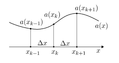
Figure 12: Sketch of the variables $a(x_{k})$ representing the random field $u(x,t;\omega)$ at $x_{k}$. When we send $\Delta x$ to zero, the number of variables $a(x_{k})$ goes to infinity and the joint probability density function becomes a probability density functional (see equation (340)).

By using well-known identities involving the Dirac delta function [107] it can be shown that

$$\frac{a(x_{k+1})-2a(x_{k})+a(x_{k-1)}}{\Delta x^{2}}\left<\prod_{k=1}^{n}\delta\left(a(x_{k})-u(x_{k},t;\omega)\right)\right>=$$

$$\left<\frac{u(x_{k+1},t;\omega)-2u(x_{k},t;\omega)+u(x_{k-1},t;\omega)}{\Delta x^{2}}\prod_{j=1}^{n}\delta\left(a(x_{j})-u(x_{j},t;\omega)\right)\right>.$$ (349)

This yields,

$$\frac{\tilde{\partial}^{2}a(x_{k})}{\tilde{\partial}x^{2}}\left<\prod_{k=1}^{n}\delta\left(a(x_{k})-u(x_{k},t;\omega)\right)\right>=\left<\frac{\tilde{\partial}^{2}u(x_{k},t;\omega)}{\tilde{\partial}x^{2}}\prod_{j=1}^{n}\delta\left(a(x_{j})-u(x_{j},t;\omega)\right)\right>,$$ (350)

where $\tilde{\partial}^{2}/\tilde{\partial}x^{2}$ is the numerical differentiation operator, i.e., the approximation of the second-order derivative operator by using finite differences, or other differentiation schemes such as pseudospectral collocation [84]. By extending these arguments to higher-order derivatives, we obtain

$$\frac{\tilde{\partial}^{s}a(x_{k})}{\tilde{\partial}x^{s}}\left<\prod_{k=1}^{n}\delta\left(a(x_{k})-u(x_{k},t;\omega)\right)\right>=\left<\frac{\tilde{\partial}^{s}u(x_{k},t;\omega)}{\tilde{\partial}x^{s}}\prod_{j=1}^{n}\delta\left(a(x_{j})-u(x_{j},t;\omega)\right)\right>,\quad s=1,2,...$$ (351)

The joint probability density function of the state vector $u(x_{i},t;\omega)$ ($i=1,...,n$) satisfies the equation [228, 227, 229]

$$\frac{\partial p}{\partial t}= -\sum_{k=1}^{n}\frac{\partial}{\partial a_{k}}\left<\frac{\tilde{\partial}^{2}u(x_{i},t;\omega)}{\tilde{\partial}x^{2}}\prod_{j=1}^{n}\delta\left(a_{j}-u(x_{j},t;\omega)\right)\right>,$$

$$= -\sum_{k=1}^{n}\frac{\partial}{\partial a_{k}}\left(\frac{\tilde{\partial}^{2}a(x_{i})}{\tilde{\partial}x^{2}}p\right),$$ (352)

where $p=p(a_{1},...,a_{n},t)$. The last equality follows from (350). By taking the continuum limit, i.e., by sending $\Delta x$ to zero (and correspondingly $n$ to infinity), we obtain the following functional differential equation for the probability density functional of the solution to equation (345)

$$\frac{\partial P([a(x)],t)}{\partial t}=-\int_{-\infty}^{\infty}\frac{\delta}{\delta a(x)}\left(\frac{\partial^{2}a(x)}{\partial x^{2}}P([a(x)],t)\right)dx.$$ (353)

This equation is in agreement with (346).

Remark: The functional equation (353) is linear in $P([a(x)],t)$, but it involves a singular term. Such term is generated by the derivative

$$\frac{\delta}{\delta a(x)}\left(\frac{\partial^{2}a(x)}{\partial x^{2}}\right)= \frac{\delta}{\delta a(x)}\int_{-\infty}^{\infty}a(y)\delta^{\prime\prime}(x-y)dy,$$

$$= \int_{-\infty}^{\infty}\delta(x-y)\delta^{\prime\prime}(x-y)dy.$$ (354)

The last integral is equivalent to the second derivative of the Dirac delta function evaluated at zero $x=0$. Such singularity can also be seen from a purely discrete viewpoint. To this end, substitute the (second-order) finite-difference approximation to the second-order derivative into (352). This yields the equation

$$\frac{\partial p}{\partial t}=-\sum_{k=1}^{n}\frac{a(x_{k+1})-2a(x_{k})+a(x_{k-1)}}{\Delta x^{2}}\frac{\partial p}{\partial a_{k}}-\frac{2}{\Delta x^{2}}p.$$ (355)

It is clear that as $\Delta x$ goes to zero (continuum limit), the term $2p/\Delta x^{2}$ generates a singularity.

Regularity of the Probability Functional

The solution to a probability functional equation may be an irregular functional. To understand why, consider Figure 12. When we send $\Delta x$ to zero we have that $x_{k}$ approaches $x_{k+1}$. Correspondingly the random variables $u(x_{k};t,\omega)$ and $u(x_{k+1};t,\omega)$ tend to be the same random variable. In this situation, the joint PDF of $u(x_{k};t,\omega)$ and $u(x_{k+1};t,\omega)$ involves a Dirac delta function as $x_{k}\rightarrow x_{k+1}$ (see [130], p. 970). In a continuum setting, the phenomenon we just described happens at each point $x$. Therefore the probability density functional can be an irregular mathematical object.

Example 1: The probability density functional of a zero mean Gaussian random function $u(x;\omega)$ ($x\in\mathbb{R}$) with covariance $C(x,y)$ is proportional to

$$P([a(x)])\sim\exp\left[-\frac{1}{2}\int_{-\infty}^{\infty}\int_{-\infty}^{\infty}C^{-1}(x,y)a(x)a(y)dxdy\right),$$ (356)

where $C^{-1}(x,y)$ is the inverse covariance function. Such inverse covariance may be obtained by solving the Fredholm integral equation of the first kind

$$\int_{-\infty}^{\infty}C(x,y)C^{-1}(y,z)dy=\delta(x-z).$$ (357)

If $C(x,y)$ is smooth then its differential inverse $C^{-1}(y,z)$ must have serious singularities in order for the integral in (357) to yield a Dirac delta function (see Table 1). If $C(x,y)$ is homogeneous, i.e., if $C(x,y)=C(x-y)$, then $C^{-1}(y,z)$ is called convolution inverse [88, 150]. This method was pioneered by Hirschman and Widder [86] in the late forties. Relevant cases of convolution inverses are summarized in Table 1. Note that the convolution inverses of smooth coavariance functions – such as the Maté rn covariance in 2D – are rough functions involving Laplacians and bi-harmonic operators applied to Dirac delta functions.

	Covariance		Inverse Covariance
Exponential (1D)	$\displaystyle\sigma^{2}e^{-|x|/h}$		$\displaystyle\frac{1}{2h\sigma^{2}}\left(\delta(x)-h\delta^{\prime\prime}(x)\right)$
Matérn (2D) (polar coordinates)	$\displaystyle\sigma^{2}rB_{1}\left(\frac{r}{h}\right)$		$\displaystyle\frac{1}{4\pi\sigma^{2}h^{2}}\left(\frac{\delta(r)}{\pi r}-2h^{2}\nabla^{2}\frac{\delta(r)}{\pi r}+h^{4}\nabla^{4}\frac{\delta(r)}{\pi r}\right)$
Exponential (3D) (polar coordinates)	$\displaystyle\sigma^{2}e^{-r/h}$		$\displaystyle\displaystyle\frac{1}{8\pi\sigma^{2}h^{3}}\left(\frac{\delta(r)}{\pi r}-2h^{2}\nabla^{2}\frac{\delta(r)}{\pi r}+h^{4}\nabla^{4}\frac{\delta(r)}{\pi r}\right)$

Table 1: Convolution inverses of well-known covariance functions [166]. Here $B_{1}$ denotes the modified Bessel function of the first kind. It is seen that the convolution inverse of smooth functions are rough functions involving Laplacians and bi-harmonic operators applied to Dirac delta functions.

However, such rough functions appear within integrals in (356), and therefore we expect some regularization. For instance, if we assume that the covariance function $C(x-y)$ is exponential (see Table 1), then from (356) we obtain

$$P([a(x)])\sim\exp\left[-\frac{1}{4h\sigma^{2}}\int_{-\infty}^{\infty}\left(a(x)^{2}+h^{2}\left[\frac{da(x)}{dx}\right]^{2}\right)dx\right].$$ (358)

Probability density functional equations represent an excellent starting point to obtain effective approximations. To this end, one needs to follow (by analogy) the route taken in classical statistical mechanics in which we start with the Liouville equation, and make approximations in order to derive an computable equation for a quantity of interest. Such coarse-graining process for functional differential equations is discussed by McComb [139] in the context of fluid turbulence. Probability density functional equations were derived and studied in the context turbulent flows by Dopazo and O’Brien [46], and Rosen [193, 197, 194].

Hopf Functionals and Probability Density Functionals: We have seen that Hopf equations and probability density functional equations are related by a functional Fourier transform. Therefore, from a purely mathematical viewpoint they are completely equivalent. However, from the viewpoint of approximation theory they are not equivalent at all. Hopf functionals may be hard to resolve due to high-frequencies related to the complex exponential. On the other hand, probability density functional equations may have non-smooth solutions. The statistical properties of a random field can be equivalently computed by using the Hopf functional or the probability density functional. In the first case, we simply need to take functional derivatives and evaluate them at $\theta(x)=0$ (see Section 2.1). In the second case, we need to compute functional integrals, i.e., integrals in an infinite number of variables. This requires requires a careful definition of the integration measure ([15], §2.2.4).

4.5 Effective Fokker-Planck Systems

Consider the stochastic dynamical system (315). Suppose we are interested in determining an evolution equation for the joint probability density function of the state vector $\bm{\psi}(t)$. To this end, we think of $\bm{\psi}(t)$ as a nonlinear functional of the random noise $\bm{f}(t)$, i.e., we can consider the map $\bm{\psi}(t)=\bm{\Psi}(t;[\bm{f}(t)])$. The specific form of $\bm{\Psi}$ depends on the system, in particular on the nonlinear map $\bm{\Lambda}(\bm{\psi},t)$ in (315). The probability density function of the $\bm{\Psi}(t;[\bm{f}(t)])$ can be expressed as a functional integral over the probability density functional of the noise (assuming it exists)

$$p(\bm{\psi},t)=\int\delta(\bm{\psi}-\bm{\Psi}(t;[\bm{f}]))P([\bm{f}])\mathcal{D}[\bm{f}],$$ (359)

where $\delta$ here is a multivariate Dirac delta function. From this expression, it is clear that the random noise $\bm{f}(t)$ determines $p(\bm{\psi},t)$, and therefore the structure of probability density function equation that evolves $p(\bm{\psi},t)$ in time. Such equation can be derived by using functional calculus. [228, 64, 82, 149], and it takes the form

$$\frac{\partial p(\bm{\psi},t)}{\partial t}+\nabla_{\bm{\psi}}\cdot\left(\bm{\Lambda}(\bm{\psi},t)p(\bm{\psi},t)+\left<\delta\left(\bm{\psi}-\bm{\Psi}(t;[\bm{f}])\right)\bm{f}(t)\right>_{\bm{f}}\right)=0,$$ (360)

where

$$\left<\delta\left(\bm{\psi}-\bm{\Psi}(t;[\bm{f}])\right)\bm{f}(t)\right>_{\bm{f}}=\int\delta(\bm{\psi}-\bm{\Psi}(t;[\bm{f}]))\bm{f}(t)P([\bm{f}])\mathcal{D}[\bm{f}].$$ (361)

The quantity (361) represents the correlation between two functionals of the random noise, namely $\delta(\bm{\psi}-\bm{\Psi}(t;[\bm{f}]))$ and the noise itself $\bm{f}(t)$. Such correlation can be disentangled by using functional integral techniques (see, e.g., [21, 228, 111]). In particular, if $\bm{f}(t)$ is Gaussian then (361) can be expressed by the well-known Furutsu-Novikov-Donsker formula [228, 69, 161, 43]. Similarly, if $\bm{f}(t)$ is Gaussian white noise then (315) is a Markovian system and the correlation (361) reduces to a simple diffusion term [228]. In this case (360) coincides with the classical Fokker-Plank equation [190]. We remark that computing the solution to (360) in the general (non-Markovian) setting is very challenging. Possible techniques rely on data-driven models that employ random paths of the SODE (315), e.g., path integral methods [81, 172, 138].

Non-Markovian Random Processes on Random Graphs

Consider a non-Markovian stochastic process $\bm{\psi}(t;\omega)\in\mathbb{R}^{n}$ evolving on a random graph with $n$ nodes (see Figure 13). Such process could model, e.g., the propagation of epidemics in interacing individuals [6, 35]. Introducing uncertainty in the graph allows us to take into account uncertainty in the interconnections between different nodes, which is fundamentally important when modeling dynamics of social networks and disease propagation.

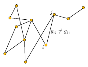
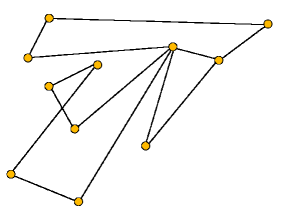
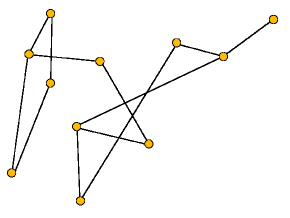
Figure 13: Samples of a random graph with fixed number of nodes. Introducing uncertainty in the edges that connect different nodes allows us to take into account uncertainty in the interactions between different components of a stochastic model evolving on the graph. This is important when modeling dynamics of social networks and disease propagation.

We can characterize a random graph mathematically in terms of random edges defined by mixed random variables, i.e., random variables with continuous/discrete probability distribution. To this end, let $g_{ij}(\omega)$ represent the interaction between the node $i$ and the node $j$, i.e., the flow of information from $i$ to $j$. Such interaction can be of different types, but roughly speaking it just characterizes how the random process $\psi_{i}(t)$ (at node $i$) influences the random process $\psi_{j}(t)$ (at node $j$). The type of influence is defined by a stochastic model on the random graph, e.g., a system of stochastic differential equations in the form

$$\frac{d\bm{\psi}}{dt}=\bm{\Lambda}(\bm{\psi},t;{\bm{G}}(\omega))+\bm{f}(t),$$ (362)

where $\Lambda$ is a nonlinear map defining the model, ${\bm{G}}(\omega)=\{g_{12}(\omega),g_{21}(\omega),...\}\in\mathbb{R}^{n(n-1)/2}$, is the random vector representing all interactions among the nodes in the random graph, and $\bm{f}(t)$ is colored random noise. The stochastic system (362) can be obviously generalized to cases where we have multiplicative noises, such as in tumororal cell growth models [248, 236, 61]. The solution to (362) (assuming it exists) is a nonlinear function of the random vector ${\bm{G}}$ defining the graph, and a nonlinear functional of the stochastic process $\bm{f}(t)$. We write such functional as $\widehat{\bm{\psi}}(t;{\bm{G}},[\bm{f}(t)])$. The probability density function of $\bm{\psi}(t)$ then can be obtained by integrating out the graph and the noise over the corresponding probability distribution, i.e.,

$$p(\bm{\psi},t)=\int\delta\left(\bm{\psi}-\widehat{\bm{\psi}}(t;{\bm{G}},[\bm{f}])\right)p({\bm{G}})P([\bm{f}])\mathcal{D}[\bm{f}]d{\bm{G}}.$$ (363)

Note that here we assumed that the noise and the graph are statistically independent. Integration over noise is (in general) a functional integral. The exact evolution equation for $p(\bm{X},t)$ can be obtained by using a functional calculus approach [228, 64, 82, 149]. This yields,

$$\frac{\partial p(\bm{\psi},t)}{\partial t}+\int\left[\nabla_{\bm{\psi}}\cdot\left(\bm{\Lambda}(\bm{\psi},t;\bm{G})p(\bm{\psi},\bm{G},t)\right)+\nabla_{\bm{\psi}}\cdot\left<\delta\left(\bm{\psi}-\widehat{\bm{\psi}}(t;\bm{G},[\bm{f}])\right)\bm{f}(t)\right>_{\bm{f}}\right]d\bm{G}=0,$$ (364)

where $p(\bm{\psi},\bm{G},t)$ is the joint probability density of $\bm{\psi}(t,\omega)$ and $\bm{G}(\omega)$, while $\left<\cdot\right>_{\bm{f}}$ is defined in (361). As before, the correlation $\left<\delta\left(\bm{\psi}-\widehat{\bm{\psi}}(t;\bm{G},[\bm{f}])\right)\bm{f}(t)\right>_{\bm{f}}$ can be disentangled by using functional calculus [21, 228, 111], or computed by using data-driven methods.

Field Equation		Functional Differential Equation
$$\frac{\partial\bm{u}}{\partial t}+(\bm{u}\cdot\nabla)\bm{u}=-\nabla p+\nu\Delta\bm{u}$$		$\displaystyle\frac{\partial\Phi([\theta],t)}{\partial t}=\sum_{k=1}^{3}\int_{V}\theta_{k}(\bm{x})\left(i\sum_{j=1}^{3}\frac{\partial}{\partial x_{j}}\frac{\delta^{2}\Phi([\bm{\theta}],t)}{\delta\theta_{k}(\bm{x})\delta\theta_{j}(\bm{x})}+\nu\nabla^{2}\frac{\delta\Phi([\bm{\theta}],t)}{\delta\theta_{k}(\bm{x})}\right)d\bm{x}$
$\displaystyle\frac{\partial u}{\partial t}+u\frac{\partial u}{\partial x}=\nu\frac{\partial^{2}u}{\partial x^{2}}$		$\displaystyle\frac{\partial P([a],t)}{\partial t}=-\int_{-\infty}^{\infty}\frac{\delta}{\delta a(x)}\left(\left[-a(x)\frac{\partial a(x)}{\partial x}+\nu\frac{\partial^{2}a(x)}{\partial x^{2}}\right]P([a],t)\right)dx$
$\displaystyle\square\phi+m^{2}\phi=\frac{\lambda}{6}\phi^{3}$		$\displaystyle\square\frac{\delta Z([a])}{\delta a(\bm{x})}+m^{2}\frac{\delta Z([a])}{\delta a(\bm{x})}-\frac{\lambda}{3!}\frac{\delta^{3}Z([a])}{\delta a(\bm{x})^{3}}-ia(\bm{x})Z([a])=0$

Table 2: Examples of functional differential equations. In this table, $\Phi$ denotes the Hopf characteristic functional, $P$ is the probability density functional, and $Z$ is the generating functional of the quantum $\phi^{4}$-theory.

4.6 Conjugate Flow Action Functionals

In a recent paper [225], we have shown how to construct an action functional for a non-potential field theory by using methods of differential geometry and nonlinear functional analysis [220, 154]. The key idea is to represent the governing equations of the field theory relative to a diffeomorphic flow of curvilinear coordinates which is assumed to be functionally dependent on the field equations, i.e., on their solution. Such flow evolves in space and time similarly to a physical fluid flow of classical mechanics and it can be chosen to symmetrize the Gâteaux derivative of the field equations relative to suitable local bilinear forms. This is equivalent to require that the governing equations of the field theory can be derived from a principle of stationary action on a flow, which we called the conjugate flow of the theory. The determining equations of the conjugate flow are functional differential equations. In particular, for a second-order nonlinear scalar field theory

$$f\left(u;u_{,\mu};u,_{\mu\nu};\widehat{x}^{\mu}_{,\nu};\widehat{x}^{\mu}_{,\nu\lambda}\right)=0,$$ (365)

we obtain

$$R^{\mu\nu}_{,\nu}+R^{\mu\nu}\Gamma^{\lambda}_{\lambda\nu}=Z^{\nu},$$ (366)

where the comma denotes differentiation with respect to the independent variable $\sigma^{\nu}$, $\Gamma^{\lambda}_{\lambda\nu}$ is the Christoffel symbol of the second kind and

$$Z^{\nu} =\frac{\partial f}{\partial u_{,\nu}}+\frac{\partial f}{\partial\widehat{x}^{\mu}_{,\nu}}\frac{\delta\widehat{x}^{\mu}}{\delta u}+\left(\frac{\partial f}{\partial\widehat{x}^{\mu}_{,\nu\rho}}+\frac{\partial f}{\partial\widehat{x}^{\mu}_{,\rho\nu}}\right)\left(\frac{\partial}{\partial\sigma^{\rho}}\frac{\delta\widehat{x}^{\mu}}{\delta u}+\frac{\delta^{2}\widehat{x}^{\mu}}{\delta u^{2}}\frac{\partial u}{\partial\sigma^{\rho}}\right),$$ (367)

$$R^{\rho\nu} =\frac{\partial f}{\partial u_{,\nu\rho}}+\frac{\partial f}{\partial\widehat{x}^{\mu}_{,\rho\nu}}\frac{\delta\widehat{x}^{\mu}}{\delta u}.$$ (368)

Given a solution to the field equation (365), the system of functional differential equations (366) allows us to identify the conjugate flow $\widehat{x}^{\mu}(\sigma^{\nu};[u])$, i.e., the functional relation between the flow $\widehat{x}^{\mu}$ and the solution $u$ for which the PDE (365) can be derived from a principle of least action (see [225] for further details). The identification of transformation groups leaving the conjugate flow action functional invariant could lead to the discovery of new conservation laws.

4.7 Large Deviation Theory and Minimum Action Methods

Large deviations theory deals with the probabilities of rare events that are exponentially small as a function of some parameter. To illustrate the theory, consider a nonlinear PDE perturbed by space-time additive random noise of small amplitude $\epsilon$

$$\frac{\partial\bm{u}}{\partial t}+\bm{G}(\bm{u})=\sqrt{\epsilon}\bm{f}(\bm{x},t;\omega).$$ (369)

We define the set trajectories connecting two arbitrary states $\{\bm{u}_{1},\bm{u}_{2}\}$

$$B=\{\bm{u}(\bm{x},t;\omega)|\quad\bm{u}(\bm{x},0;\omega)=\bm{u}_{1},\quad\bm{u}(\bm{x},T;\omega)=\bm{u}_{2}\}$$ (370)

If $\bm{f}$ is white noise, then the Freidlin-Wentzell theory gives us the following large deviation principle

$$\lim_{\epsilon\rightarrow 0^{+}}\epsilon\textrm{Pr}(\bm{u}\in B)=\inf_{\bm{u}\in B}\frac{1}{2}\int_{0}^{T}\left\|\frac{\partial\bm{u}}{\partial t}+\bm{G}(\bm{u})\right\|^{2}_{L_{2}}dt$$ (371)

where $\textrm{Pr}(A)$ denotes the probability of the event $A$, $\left\|\cdot\right\|^{2}_{L_{2}}$ indicates the $L_{2}$ norm in space. The large deviation principle is equivalent to minimum action principle

$$\min_{\begin{subarray}{c}\bm{u}(0,\bm{x};\omega)=\bm{u}_{1}\\ \bm{u}(T,\bm{x};\omega)=\bm{u}_{2}\end{subarray}}S_{T}([\bm{u}]),\qquad S_{T}([\bm{u}])=\frac{1}{2}\int_{0}^{T}\left\|\frac{\partial\bm{u}}{\partial t}+\bm{G}(\bm{u})\right\|^{2}_{L_{2}}dt.$$ (372)

The minimizer of (372) is called minimum action path, and it satisfies the functional differential equation

$$\frac{\delta S_{T}([\bm{u}])}{\delta\bm{u}(\bm{x},t)}=0\quad\bm{u}\in B.$$ (373)

The minimum action path is the most probable transition path from $\bm{u}_{1}$ to $\bm{u}_{2}$. A method to solve (373) is based on a direct discretization of $S_{T}(\bm{u})$ [48].

5 Approximation of Functional Differential Equations

In this Section we address the numerical approximation of linear FDEs in the form (300). To this end, we develop a method of weighted residuals [62, 101] in the space of functionals that allows us to derive functional least squares, functional Galerkin and functional collocation methods to FDEs is a unified and straightforward way.

5.1 The Method of Weighted Functional Residuals

The method of weighted residuals illustrates how the choice of different weight (or test) functionals can be used to construct different classes of methods extending Galerkin, least-squares and collocation methods for PDEs to functional differential equations. The general framework resembles the classical one for PDEs, in which one minimizes a residual (least-squares method) or imposes its orthogonality relative to a suitable space of test functions (Galerkin or collocation methods). To describe the weighted residuals technique, let us consider the linear functional differential equation (300). In approximating its solution numerically we are typically replacing $F([\theta],t)$ with an approximation

$$\widehat{F}([\theta],t)\simeq F([\theta],t),$$ (374)

e.g., a tensor canonical tensor decomposition (Section 3.3.1) or a Lagrangian interpolant (Section 3.2) with $N$ degrees of freedom. Substitution of the approximation (374) into equation (300) yields the (functional) residual

$$R([\theta],t)=\frac{\partial\widehat{F}([\theta],t)}{\partial t}-L([\theta],t)\widehat{F}([\theta],t)-H([\theta],t).$$ (375)

At this point, we introduce the following inner product in the space of functionals (see Appendix B)

$$\left(F,G\right)_{W}=\int F([\theta])G([\theta])W([\theta])\mathcal{D}[\theta],\qquad\textrm{(functional integral)}$$ (376)

where $W([\theta])$ is a known weight functional, and consider the set of equations

$$\left(R([\theta],t),h_{k}([\theta])\right)_{W}=0\qquad k=1,...,N$$ (377)

where $h_{k}([\theta])$ are test functionals. There is no particular restriction on $h_{k}([\theta])$. For example, they can be cardinal basis functionals, orthogonal polynomial functionals or other basis functionals. The system (377) allows us to determine the $N$ degrees of freedom in the functional approximation $\widehat{F}([\theta],t)$. Specifically, we are imposing that the residual of the FDE is orthogonal to the span of the functionals $\{h_{1},...,h_{N}\}$. The nature of the numerical scheme is determined by the choice of the test functionals $h_{j}([\theta])$ in (377).

Evaluating the functional integrals in (377) is challenging, but there are approximation methods that allow us to compute them. For example, several algorithms have been recently proposed for high-dimensional (possibly infinite-dimensional) integration [9, 176, 237, 40, 39] (see also Apendix B and Chapter 4 in [51]). The system of equations (377) defines a functional Galerkin method.

5.1.1 Functional Collocation Methods

In this class of methods the test functionals $h_{j}([\theta])$ are chosen to be Dirac delta functionals [97] centered at $\theta_{j}(x)$, i.e., $h_{j}([\theta])=\delta[\theta_{j}(x)-\theta(x)]$. In this setting, the orthogonality condition (377) can be written as

$$\int R([\theta],t)\delta[\theta_{j}(x)-\theta(x)]W([\theta])\mathcal{D}[\theta]=0\quad\Rightarrow\quad R([\theta_{j}],t)=0$$ (378)

In other words, in the functional collocation method we impose that the residual $R([\theta],t)$ vanishes at $N$ collocation nodes in $D(F)$, i.e., $N$ functions $\{\theta_{1}(x),...,\theta_{N}(x)\}$. This yields a system of $N$ equations for the unknowns $\{\alpha_{1}(t),...,\alpha_{N}(t)\}$. The solution we obtain from the functional collocation method obviously interpolates the exact solution at the nodes $\theta_{i}(x)$.

5.1.2 Functional Least Squares

In this class of methods we look for an approximate solution functional that minimizes the norm of the residual $R([\theta],t)$. Such norm may be defined in terms of the functional inner product (376), i.e., $\left\|R\right\|_{W}^{2}=(R,R)_{W}$. In this case, we obtain the following variational principle involving a functional integral

$$\min_{\widehat{F}\in D_{N}(F)}\left\|R([\theta],t)\right\|_{W}^{2}=\min_{\widehat{F}\in D_{N}(F)}\int R([\theta],t)^{2}W([\theta])\mathcal{D}[\theta].$$ (379)

The stationary points of (379) corresponding to variations of the degrees of freedom $\alpha_{k}(t)$ in (374) satisfy the the Euler-Lagrange equations

$$\left(R([\theta],t),\frac{\partial R([\theta],t)}{\partial\alpha_{k}(t)}\right)_{W}=0,\qquad k=1,...,N.$$ (380)

A comparison between (377) and (380) suggests that the test functionals $h_{j}([\theta])$ in this case are equation-dependent, i.e., they depend on the residual $R([\theta],t)$ through the formula

$$h_{k}([\theta],t)=\frac{\partial R([\theta],t)}{\partial\alpha_{k}}.$$ (381)

Remark: Error analysis, stability and consistency of functional Galerkin, functional collocation and functional least squares methods is an open question.

Remark: If we restrict $D(F)$ to a finite-dimensional function space, e.g, the span of a finite-dimensional basis, then weighted residual formulation we just discussed reduces to the weighted residual formulation for multivariate linear PDEs.

5.2 Temporal Discretization

The FDE (300) can be discretized in time with different numerical schemes such as Adams-Bashforth, Adams-Multon or BDF methods [184]. Such discretization is quite classical in numerical analysis, and it represents an important building block in the development of efficient algorithms to compute the numerical solution to FDEs. Hereafter we discuss functional tensor methods built upon explicit and implicit linear multistep schemes (see [184], p. 497). As we will see, such algorithms have significant advantages over other approaches in terms of accuracy and computational cost. Given an evenly-spaced sequence of time instants $t_{k}=k\Delta t$ ($k=0,1,...$) we write the formal solution to to the FDE (300) as

$$F([\theta],t_{n})=F([\theta],t_{n-1})+\int_{t_{n-1}}^{t_{n}}\left(L([\theta],\tau)F([\theta],\tau)+H([\theta],\tau)\right)d\tau.$$ (382)

By approximating the temporal integral with a quadrature rule we obtain a fully discrete time-integration scheme. For example, if we replace

$$S([\theta],\tau)=L([\theta],\tau)F([\theta],\tau)+H([\theta],\tau)$$ (383)

by the interpolating polynomial at $t_{n-1}$, …, $t_{n-q}$, extrapolate in $[t_{n-1},t_{n}]$, and integrate in time we obtain the $q$-th order Adams-Bashforth scheme. Hereafter we provide some examples.

5.2.1 Second-order Adams-Bashforth (AB2) method

We replace (383) with the polynomial interpolating $S([\theta],t)$ at $\{t_{n-1},t_{n-2}\}$, extrapolate such polynomial to to $[t_{n-1},t_{n}]$ and compute the integral in (382). This yields the second-order explicit explicit scheme

$$F([\theta],t_{n})=F([\theta],t_{n-1})+\frac{\Delta t}{2}\left[3S([\theta],t_{n-1})-S([\theta],t_{n-2})\right]+\Delta t\tau_{n}([\theta]),$$ (384)

where

$$\tau_{n}([\theta])=\frac{5\Delta t^{3}}{12}\frac{\partial^{3}F([\theta],t_{n-2})}{\partial t^{3}}+\mathcal{O}(\Delta t^{4}).$$ (385)

The quantity $\tau_{n}$ is the local truncation error at time $t_{n}$ ([184], p. 499). Clearly, if the operator $L([\theta],t)$ is time-independent and $H=0$, then (382) has the simpler form

$$F([\theta],t_{n})=F([\theta],t_{n-1})+\frac{\Delta t}{2}L([\theta])\left[3F([\theta],t_{n-1})-F([\theta],t_{n-2})\right]+\Delta t\tau_{n}([\theta]).$$ (386)

5.2.2 Crank-Nicolson Method

The Crank Nicolson method is an implicit second-order method of the Adams-Multon family. The scheme can be easily derived by discretizing the time integral in (382) with the trapezoidal rule. This yields

$$F([\theta],t_{n})=F([\theta],t_{n-1})+\frac{\Delta t}{2}\left[S([\theta],t_{n})+S([\theta],t_{n-1})\right]+\Delta t\tau_{n}([\theta]),$$ (387)

where

$$\tau_{n}([\theta])=-\frac{\Delta t^{3}}{12}\frac{\partial^{3}F([\theta],t_{n-1})}{\partial t^{3}}+\mathcal{O}(\Delta t^{4})$$ (388)

is the local truncation error ([184], p. 499). The scheme (387) can be rewritten as

$$\left[I-\frac{\Delta t}{2}L([\theta],t_{n})\right]F([\theta],t_{n})= \left[I+\frac{\Delta t}{2}L([\theta],t_{n-1})\right]F([\theta],t_{n-1})+$$

$$\frac{\Delta t}{2}\left[H([\theta],t_{n})+H([\theta],t_{n-1})\right]+\Delta t\tau_{n}([\theta]),$$ (389)

The integration process proceeds as follows: Given $F([\theta],t_{n-1})$ we build the right hand side of (389) and then solve for $F([\theta],t_{n})$. This involves inverting the following (functional differential) linear operator

$$A([\theta],t_{n})=\left[I-\frac{\Delta t}{2}L([\theta],t_{n})\right].$$ (390)

It is convenient to rewrite (389) as

$$A([\theta],t_{n})F([\theta],t_{n})=E([\theta],t_{n})+\Delta t\tau_{n}([\theta]),$$ (391)

where

$$E([\theta],t_{n})=\left[I+\frac{\Delta t}{2}L([\theta],t_{n-1})\right]F([\theta],t_{n-1})+\frac{\Delta t}{2}\left[H([\theta],t_{n})+H([\theta],t_{n-1})\right].$$ (392)

is a known functional, provided $F([\theta],t_{n-1})$ is known (solution at time $t_{n-1}=(n-1)\Delta t$).

5.3 Functional Approximation

The solution to the FDE (300) can be approximated at each time step by using the functional approximation methods we discussed in Section 3. For example, if we restrict the domain the solution functional $F$ to the finite-dimensional Hilbert space spanned by the orthonormal basis $\{\varphi_{1},...,\varphi_{m}\}$, i.e.,

$$D_{m}=\textrm{span}\{\varphi_{1},...,\varphi_{m}\}\subseteq D(F),$$ (393)

then the functional becomes a multivariate function. Alternatively, we can look for an approximant of $F$ in the space of cylindrical functionals. This yields a functional in the form (see Section 3.3)

$$f(a_{1},...,a_{m},t_{n})\simeq F([\theta],t_{n}),\qquad a_{k}=(\theta,\varphi_{k}).$$ (394)

For example, in a canonical tensor decomposition setting we have

$$f(a_{1},...,a_{m},t_{n})\simeq\sum_{l=1}^{r}\prod_{j=1}^{m}G_{j}^{l}(a_{j},t_{n}),\qquad G^{l}_{j}(a_{j},t_{n})=\sum_{p=1}^{P}\beta_{jp}^{l}(t_{n})\phi_{p}(a_{j}),\qquad$$ (395)

where $r$ is the separation rank. Replacing with $F([\theta],t)$ with $f(a_{1},...,a_{m},t)$ in (384) or (391) yields a functional residual $R([\theta],t_{n})$. For example, a substitution of (395) into the Crank-Nicolson scheme (391) yields

$$R([\theta],t_{n})=\sum_{l=1}^{r}A([\theta],t_{n})G^{l}_{1}((\theta,\varphi_{1}),t_{n})\cdots G^{l}_{m}((\theta,\varphi_{m}),t_{n})-E([\theta],t_{n}).$$ (396)

Note that we have incorporated the local truncation error $\Delta t\tau_{n}$ within the residual $R([\theta],t_{n})$.

5.4 CP-ALS Algorithm for FDEs with Implict Time Stepping

We have seen in Section 5.1.2 that the functional least squares fomulation of the FDE (300) relies on minimizing the norm of the residual. Such residual can have different forms. In particular, if we discretize the FDE (300) in time with the Crank-Nicolson method and represent its solution by a canonical polyadic (CP) tensor expansion then the residual takes the form (396). Its norm can be defined as

$$\left\|R([\theta],t_{n})\right\|_{W}^{2}=\left\|\sum_{l=1}^{r}A([\theta],t_{n})G^{l}_{1}((\theta,\varphi_{1}),t_{n})\cdots G^{l}_{m}((\theta,\varphi_{m}),t_{n})-E([\theta],t_{n})\right\|_{W}^{2},$$ (397)

where $\|\cdot\|^{2}_{W}$ is induced by the functional inner product (376). Recall that the functions $G_{k}^{l}((\theta,\varphi_{k}),t_{n})$ are in the form

$$G_{k}^{l}((\theta,\varphi_{k}),t_{n})=\sum_{s=1}^{Q}\beta^{l}_{ks}(t_{n})\phi_{s}((\theta,\varphi_{k})),$$ (398)

$\beta^{l}_{ks}(t_{n})$ ($l=1,...,r$, $k=1,...,m$, $s=1,...,Q$) being the degrees of freedom. We look for a minimizer of (397) computed in a parsimonious way. The key idea is to split the large scale optimization problem

$$\min_{\beta_{ks}^{l}(t_{n})}\left\|R([\theta],t_{n})\right\|_{W}^{2}$$ (399)

into a sequence of optimization problems problems of smaller dimension, which are solved sequentially and eventually in parallel [100]. To this end, we define

$$\bm{\beta}_{k}(t_{n})=[\beta^{1}_{k1}(t_{n}),...,\beta^{1}_{kQ}(t_{n}),...,\beta^{r}_{k1}(t_{n}),...,\beta^{r}_{kQ}(t_{n})]^{T}\qquad k=1,...,m.$$ (400)

Note that the vector $\bm{\beta}_{k}(t_{n})$ collects the degrees of freedom representing the solution functional along $(\theta,\varphi_{k})$ at time $t_{n}$, i.e., the set of functions $\{G_{k}^{1}((\theta,\varphi_{k}),t_{n}),...,G^{r}_{k}((\theta,\varphi_{k}),t_{n})\}$. Minimization of (397) with respect to independent variations of $\bm{\beta}_{k}(t_{n})$ yields the sequence of convex optimization problems

$$\min_{\bm{\beta}_{1}(t_{n})}\left\|R([\theta],t_{n})\right\|_{W}^{2},\qquad\min_{\bm{\beta}_{2}(t_{n})}\left\|R([\theta],t_{n})\right\|_{W}^{2},\qquad\cdots,\qquad\min_{\bm{\beta}_{m}(t_{n})}\left\|R([\theta],t_{n})\right\|_{W}^{2}.$$ (401)

This is the set of equations defining the alternating least-squares (ALS) method. The Euler-Lagrange equations identifying the stationary points of (401) are

$$\bm{M}_{h}(t_{n})\bm{\beta}_{h}(t_{n})=\bm{f}_{h}(t_{n}),\qquad h=1,...,m$$ (402)

where,

$$[\bm{M}_{h}(t_{n})]_{qs}^{zl}=\int Q_{qh}^{z}([\theta],t_{n})Q_{sq}^{l}([\theta],t_{n})W([\theta])\mathcal{D}[\theta],$$ (403)

$$[\bm{f}_{h}(t_{n})]^{z}_{q}=\int E([\theta],t_{n})Q_{qh}^{z}([\theta],t_{n})W([\theta])D[\theta],$$ (404)

$$Q_{qh}^{z}([\theta],t_{n})=A([\theta],t_{n})\phi_{q}((\theta,\varphi_{h}))\prod_{\begin{subarray}{c}j=1\\ j\neq h\end{subarray}}^{m}G_{j}^{z}((\theta,\varphi_{j}),t_{n}).$$ (405)

The ordering of the matrix elements $[\bm{M}_{h}(t_{n})]_{qs}^{zl}$ and the vector $[\bm{f}_{h}(t_{n})]^{z}_{q}$ is the same as in (207). Note that minimizing the norm of the residual (397) with respect $\bm{\beta}_{h}(t_{n})$ is equivalent to impose orthogonality of (396) with respect to the space spanned by the basis functionals $Q_{qh}^{z}([\theta],t_{n})$. Indeed, the system (402) is equivalent to

$$\left(R([\theta],t_{n}),Q_{qh}^{z}([\theta],t_{n})\right)_{W}=0\qquad\textrm{(fixed $h=1,...,m$),}$$ (406)

where $(,)_{W}$ is the functional inner product (376). The system of equations (402) is symmetric and positive definite . This allows us to use well-known high-performance algorithms to compute the solution, e.g., the conjugate gradient method ([184], p.152). It is important to emphasize that the minimization of the residual (397) is basically a fixed point problem involving the vector

$$\bm{\beta}(t_{n})=[\bm{\beta}_{1}(t_{n})\quad\cdots\quad\bm{\beta}_{m}(t_{n})]$$ (407)

The ALS method aims at solving such fixed point problem by splitting it into a sequence of linear problems (402) which are solved iteratively for each $h$. The criterion is to freeze all $\bm{\beta}_{j}(t_{n})$ ($j=1,...,m$, $j\neq h$) when solving for $\bm{\beta}_{h}(t_{n})$. We recall that convergence of CP-ALS iterations is, in general, not granted (see Section 3.3.1). To overcome this problem, additional regularization terms may be necessary [1, 12].

Evaluation of the Functional Integrals

The ALS coefficients (403) and (404) are defined by functional integrals involving cylindrical functionals. The computation of such integrals is briefly addressed in Appendix B.1. Hereafter we summarize the main results. We first restrict $\theta(x)$ to the space of functions (393), i.e., we assume that $\theta(x)$ can be written as

$${\theta}(x)=\sum_{k=1}^{m}a_{k}\varphi_{k}(x),\qquad a_{k}=(\theta,\varphi_{k}).$$ (408)

In this hypothesis, the basis functionals (405) become multivariate functions of $(a_{1},...,a_{m})$, i.e.,

$$Q^{z}_{qh}(a_{1},....,a_{m},t_{n})=A(a_{1},...,a_{m},t_{n})\phi_{q}(a_{h})\prod_{\begin{subarray}{c}j=1\\ j\neq h\end{subarray}}^{m}G_{j}^{z}(a_{j},t_{n}).$$ (409)

Similarly, the coefficients (403) and (404) can be explicitly written as multivariate integrals

$$[\bm{M}_{h}(t_{n})]_{qs}^{zl}=\int_{-b}^{b}\cdots\int_{-b}^{b}Q^{z}_{qh}(a_{1},....,a_{m},t_{n})Q^{l}_{sq}(a_{1},...,a_{m},t_{n})da_{1}\cdots da_{m},$$ (410)

$$[\bm{f}_{h}(t_{n})]^{z}_{q}=\int_{-b}^{b}\cdots\int_{-b}^{b}E(a_{1},...,a_{m},t_{n})Q^{z}_{qh}(a_{1},..,a_{m},t_{n})da_{1}\cdots da_{m},$$ (411)

The quantity $A(a_{1},...,a_{m},t_{n})$ appearing in (409) is the discrete version of the functional differential operator $A([\theta],t_{n})$, i.e., it is a linear operator in the form

$$A(a_{1},...,a_{m},t_{n})=I-\frac{\Delta t}{2}L(a_{1},...,a_{m},t_{n})$$ (412)

where $L(a_{1},...,a_{m},t_{n})$ is the finite-dimensional version of the operator $L([\theta],t_{n})$ in (300). In general, the integrals (410) and (411) can be computed numerically only for a relatively small number of variables $a_{k}$ ($k=1,...,m$). However, if we assume that the operator $A(a_{1},...,a_{m},t_{n})$ is separable, i.e.,

$$A(a_{1},...,a_{m},t_{n})=\sum_{k=1}^{r_{A}}A_{1}^{k}(a_{1},t_{n})\cdots A_{m}^{k}(a_{m},t_{n}),$$ (413)

then the cost of computing such integrals scales linearly with the dimension $m$ of the space, since (410) and (411) can be factored as products of one-dimensional integrals. In equation (413), $A_{i}^{k}(a_{i},t_{n})$ are one-dimensional linear operators, while $r_{A}$ is the separation rank of the operator $A(a_{1},...,a_{m},t_{n})$. With the operator decomposition (413) available, we can represent the multivariate fields (405) as

$$Q_{qs}^{l}(a_{1},...,a_{m},t_{n})=\sum_{k=1}^{r_{A}}A_{q}^{k}(a_{q},t_{n})\phi_{s}(a_{q})\prod_{\begin{subarray}{c}j=1\\ j\neq q\end{subarray}}^{m}A_{j}^{k}(a_{j},t_{n})G_{j}^{l}(a_{j},t_{n}).$$ (414)

This yields the following representation of the matrix coefficients (410)

$$\left[\bm{M}_{q}(t_{n})\right]_{sh}^{lz}= \int_{-b}^{b}\cdots\int_{-b}^{b}Q_{qs}^{l}(a_{1},...,a_{m},t_{n})Q_{qh}^{z}(a_{1},...,a_{m},t_{n})da_{1}\cdots da_{m}$$

$$= \sum_{k,e=1}^{r_{A}}\int_{-b}^{b}A_{q}^{k}(a_{q},t_{n})\phi_{s}(a_{q})A_{q}^{e}(a_{q},t_{n})\phi_{h}(a_{q})da_{q}\times$$

$$\prod_{\begin{subarray}{c}j=1\\ j\neq q\end{subarray}}^{m}\int_{-b}^{b}A_{j}^{k}(a_{j},t_{n})G_{j}^{l}(a_{j},t_{n})A_{j}^{e}(a_{j},t_{n})G_{j}^{z}(a_{j},t_{n})da_{j}.$$ (415)

i.e., sums of products of one-dimensional integrals. Let us provide a simple example.

Example 1: Consider the time-independent functional differential operator (302) and the associated operator defined in (390)

$$A([\theta])=I+\frac{\Delta t}{2}\int_{0}^{2\pi}\theta(x)\frac{\partial}{\partial x}\frac{\delta}{\delta\theta(x)}dx.$$ (418)

Evaluating $A([\theta])$ in the finite-dimensional function space (393) yields

$$A(a_{1},...,a_{m})=I+\frac{\Delta t}{2}\sum_{k=1}^{m}\left(\sum_{j=1}^{m}a_{j}\int_{0}^{2\pi}\varphi_{k}(x)\frac{d\varphi_{j}(x)}{dx}dx\right)\frac{\partial}{\partial a_{k}}.$$ (419)

Therefore, $A(a_{1},...,a_{m})$ is a separable operator with separation rank $r_{A}=m^{2}+1$.

5.4.1 Collocation Setting

Consider the sequence of linear systems (402), and let $\{\phi_{s}(a_{k})\}$ be a cardinal basis associated with the set of collocation nodes $\{a_{k1},...,a_{kQ}\}$. For simplicity, we consider the same set of nodes in each dimension. In this assumption, the integrals defining the the matrix entries (415) can be significantly simplified. For example,

$$\int_{-b}^{b}A_{q}^{k}(a)\phi_{s}(a)A_{q}^{e}(a)\phi_{h}(a)da\simeq\underbrace{\bm{A}_{q}^{k}\bm{W}\bm{A}_{q}^{e}}_{\bm{K}_{q}^{ke}}$$ (420)

where $\bm{A}_{q}^{k}$ is the matrix representation of the operator $A_{q}^{k}(a)$ (collocation version), and $\bm{W}$ is a diagonal matrix of integration weights. The matrix $\bm{K}_{q}^{ke}$ is $Q\times Q$ for all $k,e=1,...,r_{A}$ and all $q=1,...,m$. With $\bm{K}_{q}^{ke}$ available, it is easy to determine the matrix representation of the integral

$$\int_{-b}^{b}A_{q}^{k}(a)G^{l}_{j}(a)A_{q}^{e}(a)G_{j}^{z}(a)da=\sum_{s,h=1}^{Q}\beta_{js}^{l}\beta_{jh}^{z}\int_{-b}^{b}A_{q}^{k}(a)\phi_{s}(a)A_{q}^{e}(a)\phi_{h}(a)da\simeq\bm{\beta}_{j}^{T}\bm{K}_{q}^{ke}\bm{\beta}_{j}$$ (421)

where $\bm{\beta}_{j}$ here is a matrix that has $G_{j}^{z}(x_{jp})$ ($p=1,..,Q$) as $z$-th column. This yields the following matrix

$$\bm{M}_{q}=\sum_{k,e=1}^{r_{A}}[\bm{R}^{ke}_{q}]^{T}\otimes\bm{K}_{q}^{ke}.$$ (422)

where

$$\bm{R}^{ke}_{q}=\prod_{\begin{subarray}{c}j=1\\ j\neq q\end{subarray}}^{m}\bm{\beta}_{j}^{T}\bm{K}_{q}^{ke}\bm{\beta}_{j}.$$ (423)

5.5 Tensor Formats for FDEs with Explicit Time Stepping

Consider the following finite-dimensional form of the linear FDE (300)

$$\frac{\partial f}{\partial t}=Lf+h,$$ (424)

where $f(a_{1},..,a_{m},t)$ is a tensor format that approximates a functional $F([\theta],t)$ and $L(a_{1},...,a_{m},t)$ is the linear operator arising from the discretization of the functional linear operator $L([\theta],t)$, and $h(a_{1},...,a_{m},t)$ is the tensor format that appoximates $H([\theta],t)$. In particular, consider the case where $h=0$, $L$ is time-independent and time-integration follows the Adams-Bashforth scheme (386), i.e.,

$$f_{n}=f_{n-1}+\frac{\Delta t}{2}L\left(3f_{n-1}-f_{n-2}\right).$$ (425)

In the last equation we employed the shorthand notation $f_{n}=f(a_{1},...,a_{m},t_{n})$. Assuming, that the operator $L$ is separable, e.g.,

$$L=-\sum_{i,j=1}^{m}a_{i}C_{ij}\frac{\partial}{\partial a_{j}},$$ (426)

then a greedy computation of the tensor format $f_{n}$ involves the following steps:

1. compute a low rank representation of $\hat{f}_{n-1}=3f_{n-1}/2-f_{n-2}/2$,

2. compute a low rank representation of $f_{n}=p_{n-1}+\Delta tL\hat{f}_{n-1}$.

The need for a low rank representation is clear: any algebraic operation between tensors, including the application of a linear operator, increases the separation rank. Therefore, efficient rank reduction methods are needed to avoid an explosion of the number of terms when solving the PDE (424) with tensor methods. Among them we recall methods based on alternating least squares [100, 12, 56], hierarchical Tucker formats [76, 113] or block coordinate descent methods [245]. Disregarding the particular tensor format employed to represent the solution functional, we emphasize that the development of rubust and efficient rank-reduction algorithms is an active area of research [8, 158].

6 Numerical Results: Functionals

In this Section we provide numerical results and examples on functional approximation. In particular, we discuss polynomial functional interpolants and functional tensor methods.

6.1 Linear functionals

Consider the linear functional

$$F([\theta])=\int^{2\pi}_{0}K_{1}(x)\theta(x)dx$$ (427)

on the Hilbert space of square integrable periodic functions in $[0,2\pi]$

$$D(F)=\{\theta\in L_{2}([0,2\pi])\,|\,\theta(0)=\theta(2\pi)\}.$$ (428)

Our aim is to represent $F([\theta])$ in terms of a functional interpolant in $D(F)$, i.e.,

$$F([\theta])=\sum_{k=1}^{\infty}F([\theta_{i}])g_{i}([\theta]).$$ (429)

where $g_{i}([\theta])$ are cardinal basis functionals and $\theta_{i}(x)$ are interpolation nodes in $D(F)$. In particular, we choose $\theta_{i}(x)=\varphi_{i}(x)$ where $\{\varphi_{1}(x),\varphi_{2}(x),...\}$ is an orthonormal basis in $D(F)$. Assuming that $K_{1}(x)$ is in $D(F)$, i.e.,

$$K_{1}(x)=\sum_{k=1}^{\infty}(K_{1},\varphi_{k})\varphi_{k}(x),$$ (430)

it follows from (427) that

$$F([\theta])= \sum_{k=1}^{\infty}(K_{1},\varphi_{k})(\varphi_{k},\theta),$$

$$= \sum_{k=1}^{\infty}F([\varphi_{k}])(\varphi_{k},\theta).$$ (431)

This can be written as

$$F([\theta])=\sum_{k=1}^{\infty}F([\varphi_{k}])g_{k}([\theta]),\qquad\textrm{where}\qquad g_{k}([\theta])=(\varphi_{k},\theta).$$ (432)

Note that this representation coincides with Porter’s series expansion (112)-(113) on the index set $\mathcal{I}=\{1\}$.

6.1.1 Polynomial Functional Interpolation

Let us study numerically an interpolation problem involving a specific kernel. To this end, we set

$$K_{1}(x)=e^{\sin(x)}(1+\sin(\cos(x)-2)-\frac{1}{2}\qquad\textrm{(Fig. \ref{fig:kernel1})},$$ (433)

     (a)                                                            (b)

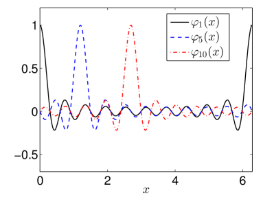
Figure 14: (a) Kernel function defining the linear functional (427). (b) Three elements of the orthogonal basis function set (434) ($m=20$).

and define the following interpolation nodes in $D(F)$

$$\varphi_{k+1}(x)=\frac{1}{m+1}\displaystyle\frac{\sin\left(\displaystyle\frac{m+1}{2}\left(x-x_{k}\right)\right)}{\sin\left(\displaystyle\frac{x-x_{k}}{2}\right)},\qquad x_{k}=\frac{2\pi}{m+1}k\qquad k=0,1,...,m$$ (434)

$m$ being an even natural number. These are well-known nodal trigonometric polynomials ([84], p. 28) satisfying the orthogonality conditions

$$(\varphi_{j},\varphi_{k})=\frac{2\pi}{m+1}\delta_{kj},\qquad k,j=1,...,m+1.$$ (435)

Clearly, if $K_{1}(x)$ is in the span of $\{\varphi_{1},...,\varphi_{m+1}\}$ then the exact representation of the linear functional $F([\theta])$ involves no more than $m+1$ terms, i.e., a truncation of the series (432) to $m+1$ terms is exact. The kernel (433) is not in such span. Next, we construct a polynomial functional that interpolates $F([\theta])$ at the nodes (434). Specifically we consider Porter’s construction (Section 3.2.3), which is very easy to implement and equivalent to Khlobystov polynomials for uniquely solvable interpolation problems. Such interpolants are dense in the space of linear functionals if we consider the set of nodes (91), i.e.,

$$\widehat{S}^{(m)}_{1}=\left\{\theta_{i}(x)\in D(F)\,\,|\,\,\theta_{i}(x)=\varphi_{i}(x)\quad i=0,...,m\right\}.$$ (436)

This means that to identify linear functionals it is sufficient to represent them relative to orthogonal bases (see Section 4.1). As we have noticed in Section 3.2.2, this is not the case for higher-order polynomial functionals or general nonlinear functionals. Now, let us consider the general expression of Porter’s interpolants

$$F\left([\theta]\right)\simeq\sum_{k=1}^{m+1}F\left([\varphi_{k}]\right)g_{k}([\theta]),\qquad g_{k}([\theta])=\sum_{j=1}^{m+1}H_{jk}^{-1}\sum_{p\in\mathcal{I}}\left(\varphi_{j},\theta\right)^{p},$$ (437)

where the matrix $H_{ij}$ is given in (111). Depending on how we choose the index set $\mathcal{I}$ we have different expressions for the basis functionals $g_{i}([\theta])$. Specifically,

1. Constant polynomial functionals ($\mathcal{I}=\{0\}$). This case is degenerate and it requires Moore-Penrose pseudo-inversion of the matrix (111). This yields the basis functionals

   $$g_{k}([\theta])=\frac{1}{m+1}.$$ (438)

2. Homogeneous polynomial functionals of first order ($\mathcal{I}=\{1\}$):

   $$g_{k}([\theta])=\left[\frac{2\pi}{m+1}\right]^{-1}\left(\theta,\varphi_{k}\right).$$ (439)

3. Quadratic polynomial functionals ($\mathcal{I}=\{1,2\}$) on the basis set $\left\{\varphi_{1},...,\varphi_{m+1}\right\}$. This yields basis functionals

   $$g_{k}([\theta])=\left[\left(\frac{2\pi}{m+1}\right)+\left(\frac{2\pi}{m+1}\right)^{2}\right]^{-1}\left(\left(\theta,\varphi_{k}\right)+\left(\theta,\varphi_{k}\right)^{2}\right).$$ (440)

In Figure 15 we plot the pointwise error

$$E_{m}=\sup_{\theta\in\mathcal{G}_{q}}\left|F([\theta])-\sum_{k=1}^{m+1}F([\varphi_{k}])g_{k}([\theta])\right|$$ (441)

versus $m$ for test functions $\theta$ in the Gaussian ensemble

$$\mathcal{G}_{q}(\sigma)=\left\{\theta(x)\in D(F)\,\left|\,\theta(x)=\sigma\sum_{k=1}^{q+1}b_{k}\varphi_{k}(x),\quad\{b_{1},...,b_{m+1}\}\quad\textrm{i.i.d. Gaussian}\right.\right\},$$ (442)

and interpolants corresponding to the index sets $\mathcal{I}=\{1\}$ and $\mathcal{I}=\{1,2\}$ (bases (439) and (440)).

     (a)                                                                     (b)

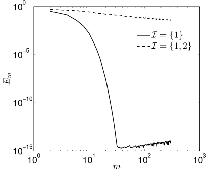
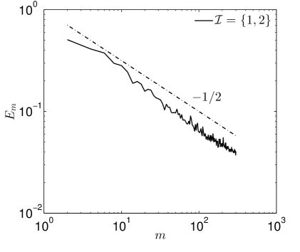
Figure 15: Linear functionals. Functional interpolation errors obtained by using Porter’s method. Shown are the pointwise errors (441) versus $m$ for the Gaussian ensemble $\mathcal{G}_{300}(1)$ and Porter’s basis functionals (439) ($\mathcal{I}=\{1\}$), and (440) ($\mathcal{I}=\{1,2\}$). The expansion corresponding to $\mathcal{I}=\{1\}$ converges exponentially for obvious reasons, while the expansion corresponding to $\mathcal{I}=\{1,2\}$ has a $O(m^{-1/2})$ convergence rate due to insufficient interpolation nodes (Fig. (b)).

The reason why we obtain exponential convergence with the index set $\mathcal{I}=\{1\}$ is obvious: convergence of the polynomial interpolant is basically defined by the convergence of the trigonometric series of $K_{1}(x)$. On the other hand, Porter’s interpolant corresponding to $\mathcal{I}={1,2}$ shows an algebraic convergence at rate $O(m^{-1/2})$. The reason is that the basis function set $\{\varphi_{1},...,\varphi_{m+1}\}$ does not have enough elements to correctly identify the quadratic part of the interpolant, which is zero in this case. In fact, the off-diagonal terms in (85) or (88) cannot be identified by using an orthogonal basis, unless we consider a set of nodes in the form $\left\{\varphi_{i},(\varphi_{i}+\varphi_{j})\right\}$ where $i,j=1,...,m+1$, and $j\geq i$.

6.1.2 Canonical Tensor Decomposition

We look for a representation of (427) in the form (187). The basis functions $G_{i}^{l}$ can be equivalently determined in an alternating Galerkin or least squares setting by solving the system of equations (206) with forcing given by

$$f^{n}_{jh}=\int_{-b}^{b}\cdots\int_{-b}^{b}\sum_{p=1}^{m+1}k_{p}a_{p}\phi_{h}(a_{j})\prod_{\begin{subarray}{c}k=1\\ k\neq j\end{subarray}}^{m+1}G^{n}_{k}(a_{k})da_{1}\cdots da_{m+1},$$ (443)

$$k_{p}=\int_{0}^{2\pi}K_{1}(x)\varphi_{p}(x)dx.$$ (444)

All integrals in (443) can be reduced to products of one-dimensional integrals (linear functionals are fully separable). In addition, if we use a polynomial basis for $G^{l}_{i}$, then we can represent (427) exactly as a product of constants and linear polynomials. In fact,

$$\sum_{l=1}^{r}G^{l}_{1}(a_{1})\cdots G^{l}_{m+1}(a_{m+1})=\sum_{l=1}^{m+1}k_{l}a_{l},$$ (445)

which means that the exact separation rank is $r={m+1}$,

$$G^{l}_{l}(a_{l})=a_{l}\qquad\textrm{and}\qquad\prod_{\begin{subarray}{c}k=1\\ k\neq l\end{subarray}}^{m+1}G_{k}^{l}(a_{k})=k_{l}.$$ (446)

6.2 Quadratic Functionals

$H_{2}(x,y)$                                               $K_{2}(x,y)$

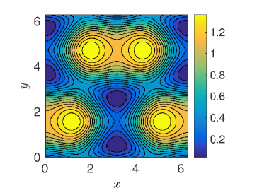
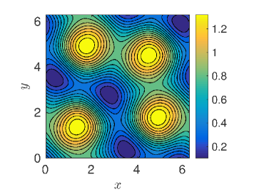
Figure 16: Quadratic functional (447). Kernel function (448) and its symmetrized version (449). Integrating $H_{2}(x,y)\theta(y)\theta(x)$ or $K_{2}(x,y)\theta(y)\theta(x)$ over $x$ and $y$ produces exactly the same result, independently on $\theta$.

Consider the quadratic functional

$$F([\theta])=5+\int^{2\pi}_{0}K_{1}(x)\theta(x)dx+\int^{2\pi}_{0}\int^{2\pi}_{0}H_{2}(x,y)\theta(x)\theta(y)dxdy$$ (447)

defined on the space of square integrable periodic functions (428). We set $K_{1}(x)$ as in (433) and $H_{2}(x,y)$ as

$$H_{2}(x,y)=\sin(\cos(x)+\sin(y))\sin(y)+\frac{1}{2}\cos(\cos(x)).$$ (448)

Replacing $H_{2}(x,y)$ with the symmetrized kernel (see Figure 16)

$$K_{2}(x,y)=\frac{1}{2}\left(H_{2}(x,y)+H_{2}(y,x)\right)$$ (449)

does not change the functional (447).

6.2.1 Polynomial Functional Interpolation

We first show that Porter’s interpolants corresponding to the index set $\mathcal{I}=\{0,1,2\}$ and Khlobystov interpolants (166) coincide when the interpolation problem is uniquely solvable, e.g., when we consider the set of nodes (92), hereafter rewritten for convenience

$$\widehat{S}^{(m+1)}_{2}=\left\{0,\{\varphi_{i}\}_{i=1}^{m+1},\{\varphi_{i}+\varphi_{j}\}_{j\geq i=1}^{m+1}\right\}.$$ (450)

In Figure 17 we plot the elements of such set for $m=10$.

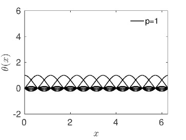
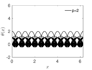
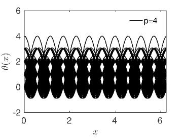
Figure 17: Interpolation nodes in the space of periodic functions (each function is a node). Here we plot the elements in the sets $\widehat{S}^{(m+1)}_{p}$ (see equation (92)) for $m=10$ and $p=1,2,3,4$. The total number of elements within each set is $\#\widehat{S}^{(11)}_{1}=12$, $\#\widehat{S}^{(11)}_{2}=78$, $\#\widehat{S}^{(11)}_{3}=364$ and $\#\widehat{S}^{(11)}_{4}=1365$.

In Figure 18 we plot the pointwise error

$$E_{m}=\sup_{\theta\in\mathcal{G}_{50}(1)}\left|F([\theta])-\Pi_{2}([\theta])\right|$$ (451)

versus $m$ for functions $\theta(x)$ in the Gaussian ensemble $\mathcal{G}_{50}(1)$ (see equation (442)). In (451), $\Pi_{2}$ represents either Porter’s or Khlobystov interpolant at the set of nodes (450).

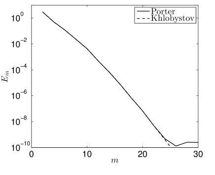
Figure 18: Interpolation of the quadratic functional (447) using Porter and Khlobystov approaches. Shown are the pointwise errors (451) versus $m$ for the Gaussian ensemble $\mathcal{G}_{50}(1)$. The small deviation between Porter’s and Khlobystov’s error plots observed at $m=24$ is due to inaccuracies in the computation of the inverse of (111). The number of interpolation nodes required to achieve accuracy of about $10^{-7}$ ($m=20$) is $\#\widehat{S}^{(21)}_{2}=253$ (see equation 93).

It is seen that both methods achieve exponential convergence rate when interpolating the polynomial functional (447). This is due to the fact that such functional expansions are basically approximating the kernel functions (433) and (448) in terms of a Fourier spectral basis. This also establishes the full equivalence of Porter’s and Khlobystov’s interpolants for uniquely solvable interpolation problems.

6.2.2 Canonical Tensor Decomposition

Evaluation of (447) in the finite-dimensional function space $D_{m}=\textrm{span}\{\varphi_{1},...,\varphi_{m+1}\}$ yields the multivariate function

$$f(a_{1},...,a_{m})=5+\sum_{p=1}^{m+1}k_{p}a_{p}+\sum_{q,p=1}^{m+1}q_{pq}a_{p}a_{q},$$ (452)

where $a_{j}=(\varphi_{j},\theta)$ and

$$k_{p}=\int_{0}^{2\pi}K_{1}(x)\varphi_{p}(x)dx,\qquad q_{pq}=\int_{0}^{2\pi}\int_{0}^{2\pi}K_{2}(x,y)\varphi_{p}(x)\varphi_{q}(x)dxdy.$$ (453)

The forcing term at the right hand side of (206) can be written as

$$f^{n}_{jh}=\int_{-b}^{b}\cdots\int_{-b}^{b}\left(5+\sum_{p=1}^{m+1}k_{p}a_{p}+\sum_{q,p=1}^{m+1}q_{pq}a_{p}a_{q}\right)\phi_{h}(a_{j})\prod_{\begin{subarray}{c}k=1\\ k\neq j\end{subarray}}^{m+1}G^{n}_{k}(a_{k})da_{1}\cdots da_{m},$$ (454)

As before, the integrals (454) can be reduced to products of one-dimensional integrals. If we use a Legendre basis $\phi_{h}$, then we can represent (447) exactly as a product of constants, linear and quadratic polynomials. To show this, let us consider the quadratic part of the functional (447). We have,

$$\sum_{l=1}^{r}G^{l}_{1}(a_{1})\cdots G^{l}_{m+1}(a_{m+1})=\sum_{q,p=1}^{m+1}q_{qp}a_{q}a_{p}.$$ (455)

Given the symmetry of $q_{pq}$, the separation rank for such quadratic part is $(m+1)(m+2)/2$. More generally, the function (452) is separable, with separation rank $r=1+(m+1)+(m+1)(m+2)/2$. In fact, it can be written in the form

$$f(a_{1},...,a_{m})=\sum_{l=1}^{r}\alpha_{l}G^{l}_{1}(a_{1})\cdots G^{l}_{m}(a_{m}).$$ (456)

A possible ordering of the series could be the one in Table 3.

$q$	$\alpha_{l}$	$G_{1}^{l}$	$G_{2}^{l}$	$\cdots$	$G_{m}^{l}$
$1$	$5$	$1$	$1$	$\cdots$	$1$
$2$	$k_{1}$	$a_{1}$	$1$	$\cdots$	$1$
$3$	$k_{2}$	$1$	$a_{2}$	$\cdots$	$1$
$\vdots$	$\vdots$	$\vdots$	$\vdots$	$\vdots$	$\vdots$
$m+2$	$k_{m+1}$	$1$	$1$	$\cdots$	$a_{m+1}$
$m+3$	$q_{11}$	$a_{1}^{2}$	$1$	$\cdots$	$1$
$m+4$	$q_{12}+q_{21}$	$a_{1}$	$a_{2}$	$\cdots$	$1$
$\vdots$	$\vdots$	$\vdots$	$\vdots$	$\vdots$	$\vdots$
$2m+4$	$q_{1(m+1)}+q_{(m+1)1}$	$a_{1}$	$1$	$\cdots$	$a_{m+1}$
$2m+5$	$q_{22}$	$1$	$a_{2}^{2}$	$\cdots$	$1$
$\vdots$	$\vdots$	$\vdots$	$\vdots$	$\vdots$	$\vdots$
$m+2+(m+1)(m+2)/2$	$q_{(m+1)(m+1)}$	$1$	$1$	$\cdots$	$a_{m+1}^{2}$

Table 3: Ordering of the terms in the canonical tensor expansion (456) of the quadratic functional (447).

In Figure 19 we study the accuracy of the canonical tensor decomposition in representing the quadratic functional (447). Specifically, we plot the relative pointwise error

$$e_{m}=\left|\frac{F([\theta])-f(a_{1},...,a_{m})}{F([\theta])}\right|\qquad a_{j}=(\theta,\varphi_{j})$$ (457)

at $\theta(x)=\sin(\cos(2x))+\sin(4x)$ versus the number of basis functions $m$ for different separation ranks.

6.2.3 Hierarchical Tucker Expansion

The hierarchical Tucker expansion aims at mitigating the dimensionality of the core-tensor of multivariate Schmidt decompositions (Section 3.3.3). It has advantages over the canonical tensor decomposition in terms of robustness and computational efficiency. In Figure 19 we study convergence of the hierarchical Tucker expansion (see Section 3.3.3) in representing the quadratic functional (447). Specifically, we plot the relative pointwise error (457) at $\theta(x)=\sin(\cos(2x))+\sin(4x)$ versus the number of dimensions $m$ for different separation ranks.

Canonical Tensor Decomposition                                   Hierarchical Tucker

       

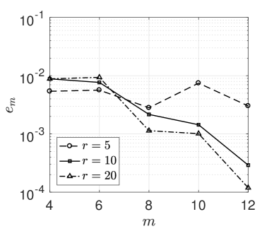
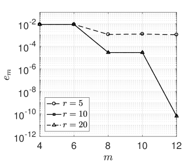
Figure 19: Accuracy of canonical tensor decomposition and hierarchical Tucker expansions in representing the quadratic functional (447). Specifically, we plot the relative pointwise error at $\theta(x)=\sin(\cos(2x))+\sin(4x)$ versus the number of dimensions $m$, and for different separation ranks.

6.3 Hopf Characteristic Functionals

In this Section we study the accuracy of polynomial functional interpolation and tensor methods in representing Hopf functionals. To this end, consider the random function

$$u_{0}(x;\omega)=\frac{1}{\sqrt{q}}\sum_{k=1}^{q}\left[\eta_{k}\sin(kx)+\xi_{k}\cos(kx)\right],$$ (458)

where $\{\eta_{k},\xi_{k}\}_{k=1,...,q}$ are i.i.d. random variables satisfying

$$\langle\xi_{k}\rangle=0,\quad\langle\eta_{k}\rangle=0,\quad\langle\xi_{k}^{2}\rangle=1,\quad\langle\eta_{k}^{2}\rangle=1.$$ (459)

In Figure 20 we plot few samples of (458), for different values of $q$ in the hypothesis that $\{\xi_{k}\}$ and $\{\eta_{k}\}$ are i.i.d. Gaussian random variables.

      $q=5$                                                $q=20$                                                $q=60$

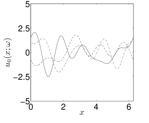
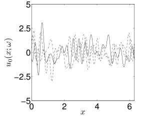
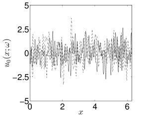
Figure 20: Samples of the random function (458) for different values of $q$ (Gaussian $\eta_{k}$ and $\xi_{k}$).

From (459) it follows that the first two statistical moments of (458) are independent of $q$, i.e., we have

$$\left<u_{0}(x;\omega)\right>=0,\qquad\left<u_{0}(x;\omega)^{2}\right>=1,\quad\textrm{for all $q$.}$$ (460)

On the other hand, the covariance function

$$C_{0}(x,y)=\frac{1}{q}\sum_{k=1}^{q}[\sin(kx)\sin(ky)+\cos(kx)\cos(ky)]$$ (461)

does depend on $q$, as shown in Figure 21. Higher-order moments and cumulants can be computed analytically in a similar way.

$q=1$                                                      $q=5$                                                      $q=20$

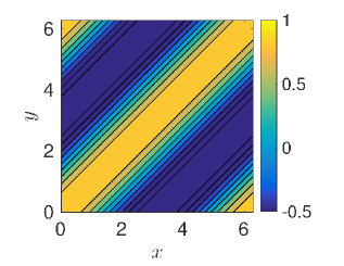
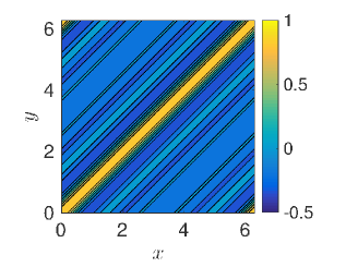
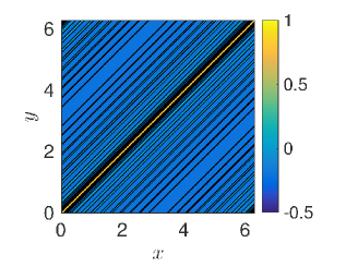
Figure 21: Covariance function (461) for different values of $q$.

The Hopf functional of $u_{0}(x;\omega)$ is defined as

$$\Phi([\theta(x)])=\left<\exp\left[i\int_{0}^{2\pi}\theta(x)u_{0}(x;\omega)dx\right]\right>,$$ (462)

where the average $\left<\cdot\right>$ is a multi-dimensional integral with respect to the joint probability density function of $\xi_{k}$ and $\eta_{k}$. By substituting (458) into (462) we obtain

$$\Phi([\theta(x)])=\prod_{k=1}^{q}\int e^{ias_{k}[\theta]}p_{\eta_{k}}(a)da\prod_{k=1}^{q}\int e^{iac_{k}[\theta]}p_{\xi_{k}}(a)da,\qquad$$ (463)

where

$$s_{k}[\theta]=\frac{1}{\sqrt{q}}\int_{0}^{2\pi}\theta(x)\sin(kx)dx,\qquad c_{k}[\theta]=\frac{1}{\sqrt{q}}\int_{0}^{2\pi}\theta(x)\cos(kx)dx.$$ (464)

Depending on the probability density functions $p_{\eta_{k}}(a)$ and $p_{\xi_{k}}(a)$ appearing in (463), we have different expressions of $F([\theta])$.

Gaussian Random Fields

Let us assume

$$p_{\eta_{k}}(a)=\frac{1}{\sqrt{2\pi}}e^{-a^{2}/2}\qquad p_{\xi_{k}}(a)=p_{\eta_{k}}(a).$$ (465)

The integrals in (463) are in the form

$$\frac{1}{\sqrt{2\pi}}\int_{-\infty}^{\infty}e^{ias_{k}[\theta]-a^{2}/2}da=e^{-s^{2}_{k}[\theta]/2}.$$ (466)

Therefore, we obtain

$$\Phi([\theta(x)])= \exp\left[-\frac{1}{2}\sum_{k=1}^{q}\left(s^{2}_{k}[\theta]+c^{2}_{k}[\theta]\right)\right]$$ (467)

$$= \exp\left[-\frac{1}{2}\int_{0}^{2\pi}\int_{0}^{2\pi}\theta(x)\theta(y)C_{0}(x,y)dxdy\right],$$ (468)

in agreement with well-known results for Hopf characteristic functionals of Gaussian random fields.

Uniform Random Fields

Let us assume

$$p_{\eta_{k}}(a)=\begin{cases}1/(2\sqrt{3})&a\in[-\sqrt{3},\sqrt{3}]\\ 0&\textrm{otherwise}\end{cases}\qquad p_{\xi_{k}}(a)=p_{\eta_{k}}(a)$$ (469)

In this way the assumptions (459) are satisfied. The integrals in (463) are easily obtained as

$$\frac{1}{2\sqrt{3}}\int_{-\sqrt{3}}^{\sqrt{3}}e^{ias_{k}[\theta]}da=\frac{\sinh(i\sqrt{3}s_{k}[\theta])}{i\sqrt{3}s_{k}[\theta]}=\frac{\sin(\sqrt{3}s_{k}[\theta])}{\sqrt{3}s_{k}[\theta]}.$$ (470)

A substitution of this formula into (463) yields

$$\Phi([\theta(x)])= \prod_{k=1}^{q}\frac{\sin(\sqrt{3}s_{k}[\theta])\sin(\sqrt{3}c_{k}[\theta])}{3s_{k}[\theta]c_{k}[\theta]}.$$ (471)

Note that in both cases we just discussed the Hopf functional turns out to be real-valued. Moreover, $\Phi\rightarrow 0$ as $\left\|\theta\right\|\rightarrow\infty$ (Riemann-Lebesgue lemma), at a rate that depends on the regularity of the underlying probability density functional. In particular, in the Gaussian case $\Phi$ goes to zero faster than in the uniform case. Note also, that both (468) are (471) are entire functionals (i.e., analytic on the complex plane). This implies that the polynomial interpolation process converges pointwise [105].

6.3.1 Effective Dimension

Let us represent $\theta(x)$ in the space of periodic functions in $[0,2\pi]$. Possible bases are the discrete trigonometric polynomials (434) or the more classical Fourier modes

$$1,\qquad\sin(kx),\qquad\cos(kx),\qquad k=1,2,....$$ (472)

Let us now ask the following question: what is the effective dimension of the Hopf functional (462) in the space of periodic functions? Such dimension is clearly determined by the dimension of the linear functionals $s_{k}$ and $c_{k}$ in (464). If we expand the test function $\theta$ in a classical Fourier series

$$\theta(x)=a_{0}+\sum_{k=1}^{N}a_{k}\sin(kx)+\sum_{k=1}^{N}b_{k}\cos(kx)$$ (473)

and we substitute it into (464) then we obtain

$$s_{k}[\theta]=\frac{\pi}{\sqrt{q}}a_{k},\qquad\textrm{and}\qquad c_{k}[\theta]=\frac{\pi}{\sqrt{q}}b_{k}.$$ (474)

This means that the effective dimension of the Hopf functional (462) is exactly $2q$. To show this numerically, we consider the Hopf functional (468) (Gaussian case) and plot the spectrum of the covariance matrix

$$Z_{ij}=\int_{0}^{2\pi}\int_{0}^{2\pi}C_{0}(x,y)\varphi_{i}(x)\varphi_{j}(y)dxdy,$$ (475)

obtained by projecting the covariance function (461) onto the the Fourier modes (472) or, equivalently, onto the discrete trigonometric polynomials (434).

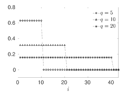
Figure 22: Spectra of the covariance matrix (475) obtained by projecting the covariance function (461) onto the Fourier modes (472), or the discrete trigonometric polynomials (434). It is seen that the number of active components is exactly $2q$ and all variables are equally important. This has important consequences when we approximate the Hopf functional using tensor methods or polynomial functionals. In particular, any approximation in a function space with less than $2q$ dimensions yields a systematic error.

As it is clearly seen from Figure 22 the number of active components is exactly $2q$. Note also that the spectrum is flat in all cases, which means that all active variables are equally important. This has important consequences when approximating the functional (468) by polynomial functionals or SSE. In particular, if we use functionals involving less than $2q$ components, e.g., if $m<2q$ in equation (187), then we cannot approximate (468) accurately, no matter how we push the expansion order.

6.3.2 Polynomial Functional Interpolation

Let us expand (468) in a power series

$$\Phi([\theta(x)])= 1-\frac{1}{2}\int_{0}^{2\pi}\int_{0}^{2\pi}C_{0}(x_{1},x_{2})\theta(x_{1})\theta(x_{2})dx_{1}dx_{2}+$$

$$\frac{1}{4}\int_{0}^{2\pi}\int_{0}^{2\pi}\int_{0}^{2\pi}\int_{0}^{2\pi}C_{0}(x_{1},x_{2})C_{0}(x_{3},x_{4})\theta(x_{1})\theta(x_{2})\theta(x_{3})\theta(x_{4})dx_{1}dx_{2}dx_{3}dx_{4}+\cdots.$$ (476)

For small $\theta(x)$ we can truncate the series, and represent $\Phi$ in terms of an interpolating polynomial functional of relatively small order, provided we have enough interpolation nodes nearby $\theta(x)=0$. This is demonstrated in Figure 23, where we study the accuracy of Porter’s interpolant through the set of nodes $\widehat{S}^{(m+1)}_{n}$ (see Eq. (92)). Specifically, we plot the error

$$E_{m}=\sup_{\theta\in\mathcal{G}_{50}(\sigma)}\left|\Phi([\theta])-\Pi_{n}([\theta])\right|$$ (477)

versus $m$ for $q=5$, $n=1,2,3,4$ and $\sigma=0.01$. It is seen that the interpolants converge in both $n$ (polynomial order) and $m$ (number of basis functions). Convergence in $m$ becomes monotonic for $m\geq 10$. This is related to the fact that the effective dimension of the Hopf functionals (467) and (471) is $10$ for $q=5$ (see Section 6.3.1). Therefore for $m\geq 10$ we have enough basis functions to fully resolve them. The accuracy of the polynomial interpolants then depends only on $n$ (polynomial order), the number of interpolation nodes and their location. The number of interpolation nodes in $\widehat{S}^{(m+1)}_{n}$ is given in (93). For example, the case $m=20$ and $n=4$ yields $12650$ nodes and an interpolation matrix (111) of size $12650\times 12650$.

      Gaussian Functional                                      Uniform Functional

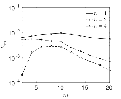
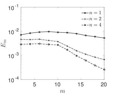
Figure 23: Accuracy of Porter’s polynomial functional interpolants in representing the Hopf functionals (467) and (471). Shown are the pointwise errors (477) versus $m$ for different orders of the polynomial interpolant. The errors are computed by sampling $20000$ functions from the set $\mathcal{G}_{50}(\sigma)$ with $\sigma=0.01$ and then computing the supremum (477).

When evaluating the error (477) it is important to select $\mathcal{G}_{50}(\sigma)$ within the convex hull of the interpolation nodes, e.g., by choosing $\sigma$ small enough. In this way we avoid inaccuracies due to polynomial extrapolation. To mitigate this phenomenon, we can also consider different sets of interpolation nodes, e.g., the set $\widetilde{S}^{(m+1)}_{n}$ defined in (96) with $a_{i_{q}}$ sampled at Gauss-Hermite sparse-grid points. In Figure 24 we plot the elements in $\widetilde{S}^{(m+1)}_{1}$, $\widetilde{S}^{(m+1)}_{2}$ and $\widetilde{S}^{(m+1)}_{3}$ for Gauss-Hermite sparse grids of level 5 (see also Table 4).

$m$	$2$	$4$	$6$	$8$	$10$	$16$	$20$
$\#\widetilde{S}^{(m+1)}_{2}$	$121$	$341$	$673$	$1117$	$1673$	$4013$	$6133$

Table 4: Number of interpolation nodes in $\widetilde{S}^{(m+1)}_{2}$ with $a_{i_{j}}$ sampled at Gauss-Hermite sparse grids (level 5).

 Nodes in Fourier space                       Nodes in function space

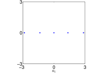
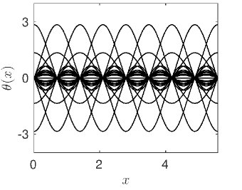
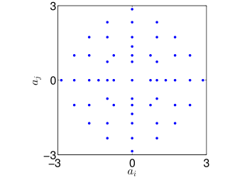
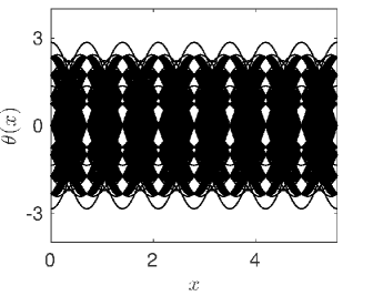
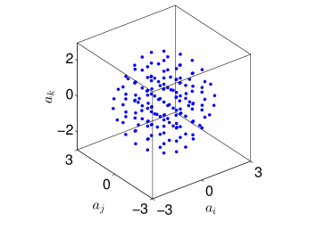
Figure 24: Gauss-Hermite sparse grids (left) and corresponding interpolation nodes in the function space $\widetilde{S}^{(m)}_{n}$ (right). Specifically, we plot all elements in $\widetilde{S}^{(9)}_{1}$ (first row, $45$ elements), $\widetilde{S}^{(9)}_{2}$ (second row, $1117$ elements) and $\widetilde{S}^{(9)}_{3}$ (third row, $3949$ elements).

The symmetry of the nodes $a_{i_{j}}$ in the Fourier space yields linearly dependent nodes in $\widetilde{S}^{(m+1)}_{n}$. Correspondingly, the interpolation matrix (111) is rank-deficient, i.e., it cannot be inverted in a classical sense. We can overcome this issue by either removing some nodes from the set $\widetilde{S}^{(m+1)}_{n}$, or by taking the More-Penrose pseudo-inverse of (111). In the latter case, we obtain a non-cardinal basis (135) and a polynomial functional in the form (134). In Figure 25 we demonstrate convergence of such polynomial functional (order 1 and 2) to the Hopf functionals (468) and (471). Specifically, we plot the pointwise errors (477) versus $m$ for a set of $20000$ randomly generated evaluation nodes in $\mathcal{G}_{50}(\sigma)$, with $\sigma=1$.

      Gaussian Functional                                             Uniform Functional

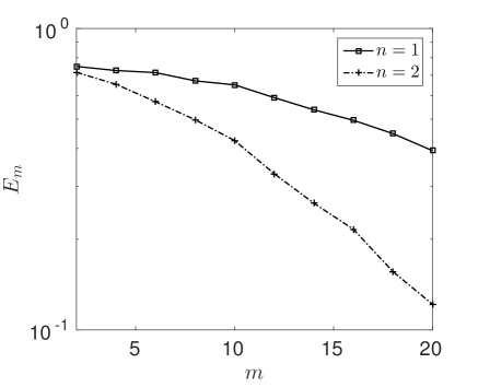
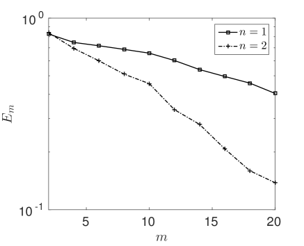
Figure 25: Approximation of the Hopf functionals (467) and (471) by using polynomial functionals of total degree $n=1$ and $n=2$. The polynomial are in the form (134) (i.e., non-interpolatory) and they are constructed by using the set of nodes $\widetilde{S}^{(m)}_{1}$ and $\widetilde{S}^{(m)}_{2}$ defined in equation (96), with $a_{i_{j}}$ sampled at Gauss-Hermite sparse grids of level $5$ [24]. Shown are the pointwise errors (477) versus $m$ for functions $\theta(x)$ in the ensemble $\mathcal{G}_{50}(1)$.

6.3.3 Canonical Tensor Decomposition

We evaluate the Hopf functionals (468) and (471) in the function space spanned by the finite-dimensional orthonormal basis

$$\varphi_{0}(x)=\frac{1}{2\pi},\quad\varphi_{k-1}(x)=\frac{\sin(kx/2)}{\sqrt{\pi}},\quad\varphi_{k}(x)=\frac{\cos((1+k/2)x)}{\sqrt{\pi}}\qquad\textrm{($k$ even)}.$$ (478)

Hereafter we prove that this yields exact rank-one representations of both Gaussian and uniform Hopf functionals.

Gaussian Functionals

By evaluating (468) in the space spanned by (478) we obtain

$$f(a_{1},...,a_{m})=\exp\left[-\frac{1}{2}\sum_{p,q=1}^{m}Z_{pq}a_{p}a_{q}\right],$$ (479)

where

$$Z_{ij}=\int_{0}^{2\pi}\int_{0}^{2\pi}C_{0}(x,y)\varphi_{i}(x)\varphi_{j}(y)dxdy.$$ (480)

It can be verified that

$$Z_{ij}=\begin{cases}\displaystyle\frac{\pi}{q}\delta_{ij}&\quad i,j\leq 2q\\ 0&\quad\textrm{otherwise}\end{cases}$$

and therefore the Gaussian functional (468) is rank one relative to the basis (478), i.e.,

$$\Phi([\theta])=\exp\left[-\frac{\pi}{2q}\sum_{p=1}^{2q}a_{p}^{2}\right],\qquad a_{p}=(\theta,\varphi_{p}).$$ (481)

Thus, a rank one canonical decomposition with $m=2q$ variables is exact in the case. It’s important to remark that the Gaussian functional (468) is not rank one relative to other bases, for example (434).

Uniform Functionals

By evaluating (471) in the space spanned by (478) we obtain

$$f(a_{1},...,a_{m})=\prod_{k=1}^{q}\frac{\sin(\sqrt{3}s_{k}(a_{1},..,a_{m}))\sin(\sqrt{3}c_{k}(a_{1},..,a_{m}))}{3s_{k}(a_{1},..,a_{m})c_{k}(a_{1},..,a_{m})},$$ (482)

where $s_{k}(a_{1},..,a_{m})$ and $c_{k}(a_{1},..,a_{m})$ are defined as (see (464))

$$s_{k}(a_{1},..,a_{m})= \frac{1}{\sqrt{q}}\sum_{p=0}^{m}(\sin(kx),\varphi_{p}(x))a_{p},$$ (483)

$$c_{k}(a_{1},..,a_{m})= \frac{1}{\sqrt{q}}\sum_{p=0}^{m}(\cos(kx),\varphi_{p}(x))a_{p}.$$ (484)

A substitution of (478) into (483)-(484) yields

$$s_{k}(a_{1},..,a_{m})= \sqrt{\frac{\pi}{q}}a_{k},\quad k=1,...,q,\quad(\textrm{zero otherwise}),$$ (485)

$$c_{k}(a_{1},..,a_{m})= \sqrt{\frac{\pi}{q}}a_{k+q},\quad k=1,...,q,\quad(\textrm{zero otherwise}).$$ (486)

This means that, relative to the basis (478) the functional (471) is rank one, i.e.,

$$\Phi([\theta])=\prod_{k=1}^{2q}\frac{\sin(\sqrt{3\pi}a_{k}/\sqrt{q})}{3\sqrt{\pi}a_{k}/\sqrt{q}},\qquad a_{k}=(\theta,\varphi_{k}).$$ (487)

Therefore, a rank one canonical tensor decomposition with $m=2q$ variables is exact. Similarly to the Gaussian case, the uniform functional is not rank-one relative to other bases, for example (434).

6.3.4 Functional Derivatives

The first- and second-order functional derivatives of the Hopf functional (462) are defined as

$$\frac{\delta\Phi([\theta])}{\delta\theta(x)} =i\left<u_{0}(x;\omega)\exp\left[i\int_{0}^{2\pi}\theta(x)u_{0}(x;\omega)dx\right]\right>,$$ (488)

$$\frac{\delta^{2}\Phi([\theta])}{\delta\theta(x)\delta\theta(y)} =-\left<u_{0}(x;\omega)u_{0}(y;\omega)\exp\left[i\int_{0}^{2\pi}\theta(x)u_{0}(x;\omega)dx\right]\right>.$$ (489)

Remarkably, these derivatives can be expressed analytically in terms of simple functions. To this end, we need a formula to compute the averages in (488) and (489). A lengthy calculation shows that

$$\frac{\delta\Phi([\theta])}{\delta\theta(x)}=\frac{i}{\sqrt{q}}\left(I^{(c)}[\theta]\sum_{k=1}^{q}\sin(kx)I^{(s)}_{k}[\theta]+I^{(s)}[\theta]\sum_{k=1}^{q}\cos(kx)I^{(c)}_{k}[\theta]\right),$$ (490)

$$\frac{\delta^{2}\Phi([\theta])}{\delta\theta(x)\delta\theta(y)}= -\frac{1}{q}\sum_{k,h=1}^{q}\left(\sin(kx)\cos(hy)I^{(s)}_{k}[\theta]I^{(c)}_{h}[\theta]+\cos(kx)\sin(hy)I^{(c)}_{k}[\theta]I^{(s)}_{h}[\theta]\right)$$

$$-\frac{1}{q}\sum_{\begin{subarray}{c}k,h=1\\ k\neq h\end{subarray}}^{q}\left(I^{(c)}[\theta]\sin(kx)\sin(hy)I^{(s)}_{kh}[\theta]+I^{(s)}[\theta]\cos(kx)\cos(hy)I^{(c)}_{kh}[\theta]\right)$$

$$-\frac{1}{q}\sum_{k=1}^{q}\left(I^{(c)}[\theta]\sin(kx)\sin(ky)J^{(s)}_{k}[\theta]+I^{(s)}[\theta]\cos(kx)\cos(ky)J^{(c)}_{k}[\theta]\right),$$ (491)

where the functionals $I^{(c)}[\theta]$, $I^{(s)}[\theta]$, $I_{k}^{(c)}[\theta]$, etc., are defined in Table 5. These expressions are general and they hold for any random function in the form (458), with i.i.d. random variables $\eta_{k}$ and $\xi_{j}$.

Coefficients Appearing in the Functional Derivatives (490) and (491)

$\displaystyle G_{n}(z)=\int_{-\infty}^{\infty}a^{n}e^{iza}p(a)da$

Gaussian PDF $G_{0}(z)=e^{-z^{2}/2}$ $G_{1}(z)=ize^{-z^{2}/2}$ $G_{2}(z)=(1-z^{2})e^{-z^{2}/2}$ Uniform PDF $\displaystyle G_{0}(z)=\frac{\sin(\sqrt{3}z)}{\sqrt{3}z}$ $\displaystyle G_{1}(z)=i\frac{\sin(\sqrt{3}z)}{\sqrt{3}z^{2}}-i\frac{\cos(\sqrt{3}z)}{z}$ $\displaystyle G_{2}(z)=\frac{2\cos(\sqrt{3}z)}{z^{2}}+\frac{\sqrt{3}\sin(\sqrt{3}z)}{z}-\frac{2\sin(\sqrt{3}z)}{\sqrt{3}z^{3}}$

$\displaystyle I^{(s)}[\theta]=\prod_{r=1}^{q}G_{0}(s_{r}[\theta])$ $\displaystyle I^{(c)}[\theta]=\prod_{r=1}^{q}G_{0}(c_{r}[\theta])$ $\displaystyle I_{k}^{(s)}[\theta]=G_{1}(s_{k}[\theta])\prod_{\begin{subarray}{c}r=1\\ r\neq k\end{subarray}}^{q}G_{0}(s_{r}[\theta])$ $\displaystyle I_{k}^{(c)}[\theta]=G_{1}(c_{k}[\theta])\prod_{\begin{subarray}{c}r=1\\ r\neq k\end{subarray}}^{q}G_{0}(c_{r}[\theta])$ $\displaystyle J_{k}^{(s)}[\theta]=G_{2}(s_{k}[\theta])\prod_{\begin{subarray}{c}r=1\\ r\neq k\end{subarray}}^{q}G_{0}(s_{r}[\theta])$ $\displaystyle J_{k}^{(c)}[\theta]=G_{2}(c_{k}[\theta])\prod_{\begin{subarray}{c}r=1\\ r\neq k\end{subarray}}^{q}G_{0}(c_{r}[\theta])$ $\displaystyle I_{kh}^{(s)}[\theta]=G_{1}(s_{k}[\theta])G_{1}(s_{h}[\theta])\prod_{\begin{subarray}{c}r=1\\ r\neq k,h\end{subarray}}^{q}G_{0}(s_{r}[\theta])$ $\displaystyle I_{kh}^{(c)}[\theta]=G_{1}(c_{k}[\theta])G_{1}(c_{h}[\theta])\prod_{\begin{subarray}{c}r=1\\ r\neq k,h\end{subarray}}^{q}G_{0}(c_{r}[\theta])$

Table 5: Coefficients appearing in the functional derivatives (490) and (491).

Note that in the case of uniform PDF the coefficients in Table 5 satisfy

$$\lim_{z\rightarrow 0}G_{0}(z)=1,\qquad\lim_{z\rightarrow 0}G_{1}(z)=0,\qquad\lim_{z\rightarrow 0}G_{2}(z)=1.$$ (492)

and therefore there are no singularities at $z=0$. Also, all coefficients decay to $0$ when $z$ goes to infinity. The expressions (490) and (491) can be simplified significantly for Gaussian Hopf functionals (468). In particular, we obtain

$$\frac{\delta\Phi([\theta])}{\delta\theta(x)}=-\left[\int_{0}^{2\pi}C_{0}(x,y)\theta(y)dy\right]\exp\left[-\frac{1}{2}\int_{0}^{2\pi}\int_{0}^{2\pi}C_{0}(x,y)\theta(x)\theta(y)dxdy\right],$$ (493)

$$\frac{\delta^{2}\Phi([\theta])}{\delta\theta(x)\delta\theta(y)}= \left[-C_{0}(x,y)+\int_{0}^{2\pi}C_{0}(x,y)\theta(y)dy\int_{0}^{2\pi}C_{0}(x,y)\theta(x)dx\right]\times$$

$$\exp\left[-\frac{1}{2}\int_{0}^{2\pi}\int_{0}^{2\pi}C_{0}(x,y)\theta(x)\theta(y)dxdy\right].$$ (494)

In Figure 26 and Figure 27 we plot the first- and second-order functional derivatives of the Hopf functionals (467) and (471), evaluated at different test functions.

Gaussian                                           Uniform

$\theta(x)=0$

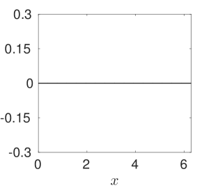
$\theta(x)=40\sin(6x)^{2}+5\cos(x)^{4}$

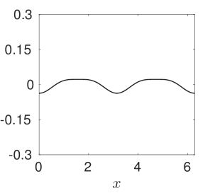
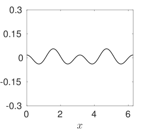
$\theta(x)=2\exp(-\sin(4x))+\cos(\cos(4x))$

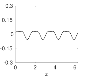
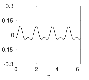
Figure 26: First-order functional derivatives of the Hopf functionals (467) (Gaussian) and (471) (Uniform) for $q=10$ evaluated at different test functions. The Hopf functionals we are considering here are real-valued and therefore the functional derivatives are real. Note that evaluating the first-order functional derivative at $\theta(x)=0$ (first row) yields the mean field $\left<u_{0}(x)\right>=0$.

Gaussian                                                Uniform

$\theta(x)=0$

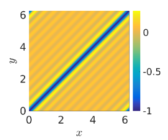
$\theta(x)=40\sin(6x)^{2}+5\cos(x)^{4}$

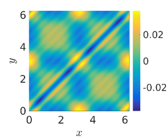
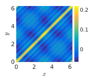
$\theta(x)=2\exp(-\sin(4x))+\cos(\cos(4x))$

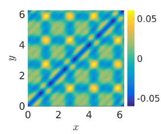
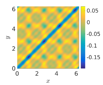
Figure 27: Second-order functional derivatives of the Hopf functionals (467) (Gaussian) and (471) (Uniform) for $q=10$ evaluated at different test functions. Both functionals are real-valued and therefore the functional derivatives are real. Note that evaluating the second-order functional derivative at $\theta(x)=0$ (first row) yields the opposite of the correlation function $C_{0}(x,y)$ in (461).

Canonical Tensor Expansion of Functional Derivatives

We have seen in Section 3.3 that the functional derivatives of any cylindrical approximant of $\Phi$ can be expressed as

$$\frac{\delta{\Phi}([\theta])}{\delta\theta(x)}\simeq\sum_{k=1}^{m}\frac{\partial f}{\partial a_{k}}\varphi_{k}(x),$$ (495)

$$\frac{\delta^{2}{\Phi}([\theta])}{\delta\theta(x)\delta\theta(y)}\simeq\sum_{k,j=1}^{m}\frac{\partial^{2}f}{\partial a_{k}\partial a_{j}}\varphi_{k}(x)\varphi_{j}(y),$$ (496)

where $a_{k}=(\theta,\varphi_{k})$. In particular, if we consider a canonical tensor expansion of $\Phi$ then $f$ has the form (187), and the partial derivatives in (495) and (496) can be easily computed. In Figure 28 we show that (495) and (496) provide a very accurate approximation of the functional derivatives (493) and (494).

                Analytical                                  Canonical Tensor Decomposition

                

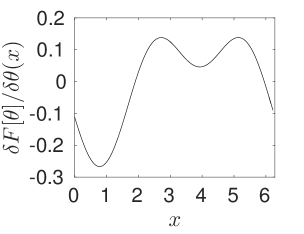
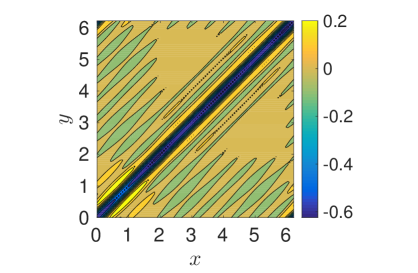
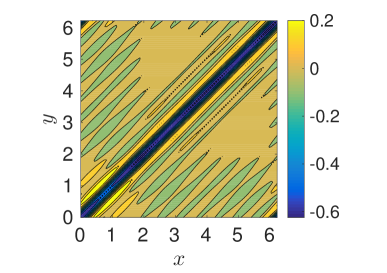
Figure 28: First- and second-order functional derivatives of the Gaussian Hopf functional (468) evaluated at $\theta(x)=\sin(x)+\sin(2x)+\sin(3x)$ . Shown are analytical results (493) and (494) versus numerical result obtained by the canonical tensor decomposition (equations (495) and (496)).

6.4 Sine Functional

Consider the nonlinear functional

$$F([\theta])=\sin\left((K_{1},\theta)\right),\qquad(K_{1},\theta)=\int_{0}^{2\pi}K_{1}(x)\theta(x)dx,$$ (497)

where $K_{1}(x)$ is as in equation (433). We represent $F([\theta])$ in the function space

$$D_{m}=\textrm{span}\{\varphi_{1},...,\varphi_{m}\}$$ (498)

spanned by a finite-dimensional orthonormal basis. This yields the cylindrical representation (see Section 3.3)

$$f(a_{1},...,a_{m})=\sin\left(\sum_{k=1}^{m}s_{k}(\varphi_{k},\theta)\right),\qquad s_{k}=\int_{0}^{2\pi}K_{1}(x)\varphi_{k}(x)dx.$$ (499)

In Figure 29 we study the accuracy of second-order Porter’s polynomial functionals and canonical tensor decomposition (187) in approximating the functional (499).

         Polynomial functionals                                Canonical Tensor Decomposition

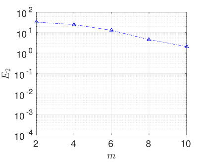
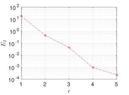
Figure 29: Approximation of the sine functional (499). Shown are the $L_{2}([-1,1]^{m})$ errors obtained by using Porter’s polynomial functionals (134) of second-order (left) with non-cardinal basis, and canonical tensor decomposition (right). Specifically, we study convergence as a function of the number of interpolation nodes in Porter’s method: $m=10$ and sparse grids level 5 yields $\#\widetilde{S}^{(m+1)}_{2}=1673$ nodes (see Table 4). In the canonical tensor decomposition method we show convergence of (187) as a function of the separation rank ($r$). The dimension of the test function space is chosen to be $m=10$.

Specifically, the polynomial functionals are constructed by using the set of nodes $\widetilde{S}^{(m+1)}_{2}$ defined in equation (92), where $a_{i_{j}}$ are sampled at Gauss-Hermite sparse grids of level 5. We recall that this set yields a rank-deficient matrix (111), which requires More-Penrose pseudoinversion (see Section 6.3.2). Correspondingly, the polynomial functionals do not interpolate (499). The canonical tensor decomposition, on the other hand, is based on Legendre polynomials of order $Q=6$. The functionals $G^{l}_{k}((\theta,\varphi_{k}))$ are shown in Figure 30.

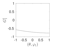
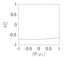
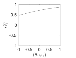
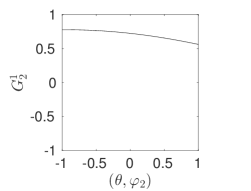
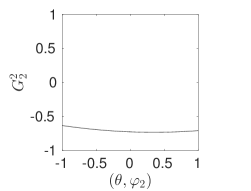
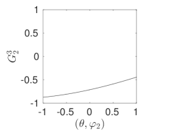
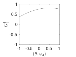
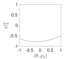
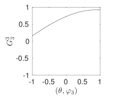
Figure 30: Tensor components of the sine functional (499) versus $(\theta,\varphi_{k})$.

6.4.1 Functional Derivatives

The first- and second-order functional derivatives of (497) are easily obtained as

$$\frac{\delta F([\theta])}{\delta\theta(x)}=K_{1}(x)\cos((K_{1},\theta)),$$ (500)

$$\frac{\delta^{2}F([\theta])}{\delta\theta(x)\delta\theta(y)}=-K_{1}(x)K_{1}(y)\sin((K_{1},\theta)).$$ (501)

Note that for each $\theta(x)$, such functional derivatives are basically a rescaled version of the functions $K_{1}(x)$ and $K_{1}(x)K_{1}(y)$. In Figure 31 we compare the exact functional derivatives versus those obtained by the canonical tensor decomposition with separation rank $r=4$.

            Analytical                                   Canonical Tensor Decomposition

                

         

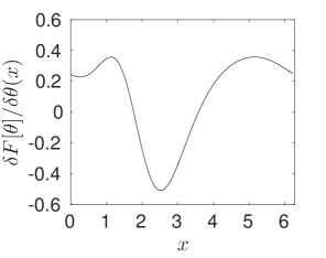
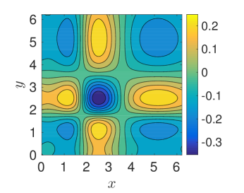
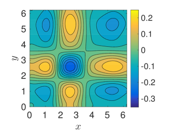
Figure 31: Sine functional (497). First- and second-order functional derivatives evaluated at $\theta(x)=9(1+\sin(x)+\sin(2x))/10$. Specifically, we compare the analytical results (500) and (501) versus results obtained by canonical tensor decomposition (equations (183) and (185)).

Recall that the functional derivatives can be approximated in the space of cylindrical functionals as (see Section 3.3)

$$\frac{\delta{F}([\theta])}{\delta\theta(x)}=\sum_{k=1}^{m}\frac{\partial f}{\partial a_{k}}\varphi_{k}(x),$$ (502)

$$\frac{\delta^{2}{F}([\theta])}{\delta\theta(x)\delta\theta(y)}=\sum_{k,j=1}^{m}\frac{\partial^{2}f}{\partial a_{k}\partial a_{j}}\varphi_{k}(x)\varphi_{j}(y).$$ (503)

In the case of canonical tensor expansions, $\partial f/\partial a_{k}$ and $\partial^{2}f/\partial a_{j}\partial a_{k}$ are defined in (198) and (199), respectively.

7 Numerical Results: Functional Differential Equations

Computing the numerical solution to a functional differential equation is a long standing open problem in mathematical physics. In this Section we address this problem with reference to linear functional equations in the form (300). In particular, we study the initial value problem for a prototype functional advection-reaction equation. We also develop the numerical discretization of the Navier-Stokes-Hopf functional equation (see Section 1), and discuss its computational complexity.

7.1 Advection-Reaction Functional Differential Equation

Consider the following advection-reaction functional differential equation

$$\frac{\partial F([\theta],t)}{\partial t}+\int_{0}^{2\pi}\theta(x)\frac{\partial}{\partial x}\left(\frac{\delta F([\theta],t)}{\delta\theta(x)}\right)dx=H([\theta],t)$$ (504)

evolving from the initial condition

$$F([\theta],0)=F_{0}([\theta]).$$ (505)

Here $H([\theta],t)$ is a given functional reaction term. We assume that $D(F)$ (the domain of the functional $F$) is a suitable space of functions, e.g., the space of periodic functions in $[0,2\pi]$ or the space of infinitely differentiable functions in $[0,2\pi]$ such that $\theta(0)=0$. Evaluation of $F([\theta],t)$ and $H([\theta],t)$ in the finite-dimensional subspace

$$D_{m}=\left\{\theta(x)\in D(F)\,\left|\,\theta(x)=\sum_{k=1}^{m}a_{k}\varphi_{k}(x)\right.\right\}\subseteq D(F),$$ (506)

where $\{\varphi_{1},...,\varphi_{m}\}$ is an orthonormal basis, yields the following multivariate functions

$$f(a_{1},...,a_{m},t)=F([\theta],t)\qquad h(a_{1},...,a_{m},t)=H([\theta]),\qquad\theta\in D_{m}.$$ (507)

We also recall that the functional derivative $\delta F([\theta],t)/\delta\theta(x)$ can be expressed in $D_{m}$ as (see Eq. (67))

$$\frac{\delta F([\theta],t)}{\delta\theta(x)}=\sum_{j=1}^{m}\frac{\partial f}{\partial a_{j}}\varphi_{j}(x).$$ (508)

A substitution of these expression back into (504) yields the following initial value problem for a multivariate first-order PDE

$$\frac{\partial f}{\partial t}+\sum_{j=1}^{m}\left(\sum_{k=1}^{m}C_{jk}a_{k}\right)\frac{\partial f}{\partial a_{j}}=h,\qquad f(a_{1},...,a_{m},0)=f_{0}(a_{1},...,a_{m}),$$ (509)

where

$$C_{jk}=\int_{0}^{2\pi}\varphi_{k}(x)\frac{d\varphi_{j}(x)}{dx}dx$$ (510)

The entries $C_{ij}$ depend on the choice of $D(F)$, and correspondingly $D_{m}$. For instance, if we assume that $D(F)$ is the space of infinitely differentiable periodic functions in $[0,2\pi]$ then the matrix (510) is centro-skew-symmetric.

Example 1: Another example of advection FDE is

$$\frac{\partial F}{\partial t}+\int_{0}^{2\pi}\theta(x)\frac{\partial}{\partial x}\left[\frac{\delta F}{\delta\theta(x)}\right]dx=\int_{0}^{2\pi}\theta(x)\frac{\partial^{2}}{\partial x^{2}}\left[\frac{\delta F}{\delta\theta(x)}\right]dx.$$ (511)

The discrete form such equation is

$$\frac{\partial f}{\partial t}+\sum_{k,j=1}^{m}a_{k}\left(C_{jk}-F_{jk}\right)\frac{\partial f}{\partial a_{j}}=0,$$ (512)

where $C_{jk}$ is defined in (510) while

$$F_{kj}=\int_{0}^{2\pi}\varphi_{k}(x)\frac{d^{2}\varphi_{j}(x)}{dx^{2}}dx.$$ (513)

7.1.1 Analytical Solution

The analytical solution to the initial value problem (509) can be computed by using the method of characteristics [189]. To this end, let $\bm{C}$ be the matrix with entries (510), and $\bm{a}$ be the vector of coordinates $(a_{1},...,a_{m})$. Then the solution to (509) is

$$f(\bm{a},t)=f_{0}\left(e^{-t\bm{C}}\bm{a}\right)+\int_{0}^{t}h\left(e^{s\bm{C}}\bm{a}\right)ds.$$ (514)

In the particular case where the reaction term $h$ is zero we obtain

$$f(a_{1},...,a_{m},t)=f_{0}\left(a_{1}(t),...,a_{m}(t)\right),$$ (515)

where the (inverse) flow map $a_{i}(t;a_{1},...,a_{m})$ is given by

$$a_{i}(t;a_{1},...,a_{m})=\sum_{j=1}^{m}Z_{ij}(t)a_{j},\qquad\bm{Z}(t)=e^{-t\bm{C}}.$$ (517)

The solution to the functional equation (504) can be obtained by taking the continuum limit of (515), i.e., by sending $m$ to infinity. This yields

$$F([\theta],t)=F_{0}([\theta(x,t)]),$$ (518)

where

$$\theta(x)=\sum_{k=1}^{\infty}a_{k}\varphi_{k}(x),\qquad\theta(x,t)=\sum_{k=1}^{\infty}a_{k}(t)\varphi_{k}(x).$$ (519)

The coefficients $a_{k}(t)$ are obtained by applying the semigroup $Z_{ij}(t)$ to $a_{k}$ (see equation (517)). The analytical expression (518) can be written more rigorously in terms of the action of a semigroup $U(t)$ [52] to $\theta(x)$, i.e.,

$$F([\theta],t)=F_{0}([U(t)\theta(x)]).$$ (520)

As we will see, such semigroup defines a translation in the space of functions $D(F)$. Such translation can be generated by rotations or contractions, depending on the space of functions $D(F)$ we consider. Hereafter we discuss this matter in more detail.

Periodic Function Spaces

Assume that the function space $D(F)$ (domain of the solution functional $F$), is the space of infinitely differentiable periodic functions in $[0,2\pi]$. In this case, the matrix $C_{ij}$ defined in (510) is skew-symmetric, thanks to the periodicity of $\varphi_{k}$ (just integrate (510) by parts ). Therefore, by the spectral theorem, $C_{ij}$ it has purely imaginary eigenvalues $\lambda_{k}=ki$, $k\in\mathbb{Z}$. Since $\bm{C}$ is skew-symmetric we have that $\exp[-t\bm{C}]$ is orthogonal, i.e., it defines an isometry in $\mathbb{R}^{m}$. Such isometry generates a translation in the space of periodic functions with group velocity equal to one. In other words, we have

$$\theta(x,t)=\theta(x-t).$$ (521)

Therefore, the analytical solution to the functional differential equation (504) (with $H=0$) in the space of periodic functions $D(F)$ is

$$F([\theta],t)=F_{0}([\theta(x-t)]).$$ (522)

From this equation, we see that if $F_{0}$ is invariant under translation, i.e., $F_{0}([\theta(x-t)])=F_{0}([\theta(x)])$ then the solution functional is constantly equal to the initial condition $F_{0}([\theta])$. This is discussed in more detail the following two examples.

Example 1: Consider the initial condition

$$F_{0}([\theta])=\sin\left(\int_{0}^{2\pi}\theta(x)dx\right).$$ (523)

We have seen in Section 3.1.2 that this nonlinear functional is approximable by a one-dimensional function relative to the standard Fourier (modal) basis in $[0,2\pi]$. Specifically, we obtained

$$f_{0}(a_{0},...,a_{m})=\sin\left(\sqrt{2\pi}a_{0}\right),$$ (524)

independently on $m$. This implies that the analytical solution to the initial value problem (509) is

$$f(a_{0},...,a_{m},t)=\sin\left(\sqrt{2\pi}\sum_{k=0}^{m}Z_{0k}(t)a_{k}\right),\quad\textrm{where}\quad Z_{0k}(t)=\left[e^{-t\bm{C}}\right]_{0k}.$$ (525)

It can be shown that if we sort the basis elements as in (72) then $Z_{0k}(t)=\delta_{k0}$. Therefore, the solution to (504)-(523) (with $H=0$) in the space of periodic functions is

$$F([\theta],t)=F_{0}([\theta]);$$ (526)

i.e., the constant functional. In general, the solution to a FDE is independent on the way represent the test function space $D(F)$. Thus, it shouldn’t be surprising that we obtain exactly the same result if we consider a finite-dimensional expansion in terms of nodal trigonometric polynomials. In this case, the initial condition functional can be discretized as

$$f_{0}(a_{0},...,a_{m})=\sin\left(\eta\sum_{k=0}^{m}a_{k}\right),\quad\textrm{where}\quad\eta=\int_{0}^{2\pi}\varphi_{k}(x)dx=\left(\frac{2\pi}{m+1}\right)$$ (527)

and the solution is

$$f(a_{0},...,a_{m},t)=\sin\left(\eta\sum_{k=0}^{m}a_{k}(t)\right),$$ (528)

where $a_{k}(t)$ is defined in (525). Since $\exp(-t\bm{C})$ is an orthogonal matrix we have that

$$\sum_{k=0}^{m}a_{k}(t)=\sum_{k=0}^{m}a_{k}.$$ (529)

In the limit $m\rightarrow\infty$ (528) and (529) imply (526). Such result can also be obtained by directly noting that if $\theta$ is periodic in $[0,2\pi]$ then

$$\int_{0}^{2\pi}\theta(x)dx=\int_{0}^{2\pi}\theta(x-t)dx\qquad\textrm{for all $t\in\mathbb{R}$.}$$ (530)

Substituting this into (523) and (522) yields (526).

Example 2: Consider the initial condition

$$F_{0}([\theta])=\exp\left[-\int_{0}^{2\pi}\theta(x)^{2}dx\right].$$ (531)

where $\theta(x)$ is in the space of infinitely differentiable periodic functions in $[0,2\pi]$. Represent $\theta(x)$ in a finite-dimensional space spanned by any orthonormal periodic basis in $[0,2\pi]$. This yields the following multivariate function corresponding to $F_{0}([\theta])$ (see also Section 3.1.2)

$$f_{0}(a_{1},...,a_{m})=\prod_{k=1}^{m}e^{-a_{k}^{2}}.$$ (532)

The analytical solution to the multivariate PDE (509) with initial condition (532) and $h=0$ is (see equation (515))

$$f(a_{1},...,a_{m},t)=\prod_{k=1}^{m}e^{-a_{k}(t)^{2}},$$ (533)

where

$$a_{k}(t)=\sum_{j=1}^{m}Z_{kj}(t)a_{j}\qquad\textrm{and}\qquad Z_{kj}(t)=\left[e^{-t\bm{C}}\right]_{kj}.$$ (534)

In a collocation setting where the the basis functions are normalized nodal trigonometric polynomials it is easy to see that

$$f(a_{1},...,a_{m},t)=f(a_{1},...,a_{m})\qquad\textrm{for all $t\geq 0$}$$ (535)

In fact, $a_{j}$ are the rescaled values of $theta(x)$ at node $x_{j}\in[0,2\pi]$, the rescaling coefficient being the norm of the trigonometric polynomial. Since $\theta(x)$ is periodic, when $t$ increases we have that values $a_{j}$ are just shifted to another location in $[0,2\pi]$, leaving the product in (533) constant. In other words, the solution to the FDE (504) (with $H=0$) corresponding to the initial condition (531) is

$$F([\theta],t)=F_{0}([\theta]),$$ (536)

i.e., the constant functional. As before, this result can be obtained by noting that if $\theta(x)$ is periodic in $[0,2\pi]$ then

$$\int_{0}^{2\pi}\theta(x)^{2}dx=\int_{0}^{2\pi}\theta(x-t)^{2}dx\qquad\textrm{for all $t\in\mathbb{R}$.}$$ (537)

A substitution of (537) into (531) yields (536).

Polynomial Function Spaces

To obtain non-trivial solutions to equation (504), we consider the following space of functions

$$D(F)=\left\{\theta\in{C}^{\infty}([0,2\pi])\,|\,\theta(0)=0\right\}$$ (538)

and the initial condition (531). We generate an orthonormal polynomial basis spanning $D(F)$ by orthonormalizing the modified Chebyshev basis $xT_{k}(x/\pi-1)$ in $[0,2\pi]$ though the Gram-Schmidt procedure. The basis functions we obtain are shown in Figure 32.

(a)                                             (b)                                           (c)

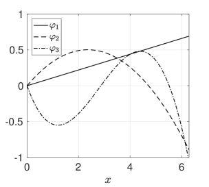
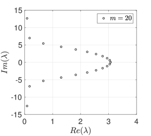
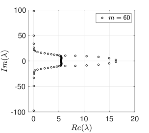
Figure 32: (a) First three orthonormal polynomial basis functions spanning the function space (538); (b)-(c) spectrum of the matrix (510) for different number of variables $m$.

This allows us to define the finite-dimensional function space

$$D_{m}=\left\{\theta\in C^{\infty}([0,2\pi])\,|\,\theta(x)=\sum_{k=1}^{m}a_{k}\varphi_{k}(x)\right\}\subseteq D(F),$$ (539)

where $\varphi_{k}$ are the orthonormal basis functions shown in Figure 32. The matrix $C_{ij}$ in this case is not skew-symmetric, and it has eigenvalues with positive real part (see Figure 32). This implies that $\bm{Z}(t)=\exp[-t\bm{C}]$ is a contraction map that takes any function $\theta(x)\in D(F)$ and continuously deforms it to $\theta(x)=0$ (see Figure 33).

(a)                                                     (b)

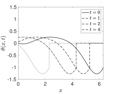
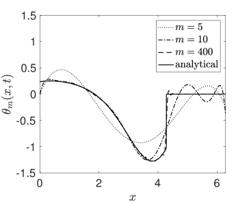
Figure 33: (a) Evolution of $\theta(x)=x\exp[-\sin(x/2)^{2}]\cos(x+4)/4$ under the (infinite-dimensional) semigroup generated by the FDE (504), i.e, $U(t)\theta(x)$ (see Eq. (520)); (b) Convergence of $\theta_{m}(x,t)$ to $\theta(x,t)$ as we increase the number of dimensions $m$ at $t=2$.

From a dynamical system viewpoint, $\exp[-t\bm{C}]\bm{a}$ is in fact stable spiral. This means that if we set the initial condition as in (533), then we obtain $f(a_{1},...,a_{m},t)\rightarrow 1$ everywhere as $t\rightarrow\infty$. The speed at which $f$ goes to one can be bounded by the spectral radius of $\bm{C}$. The solution to the functional equation (504), with initial condition (531) is

$$F([\theta],t)=\exp\left[-\int_{0}^{2\pi}\theta(x,t)^{2}dx\right],$$ (540)

where $\theta(x,t)$ is defined in (519). More explicitly,

$$F([\theta],t)=\begin{cases}\displaystyle\exp\left[-\int_{t}^{2\pi}\theta(x)^{2}dx\right]&t\in[0,2\pi]\\ \displaystyle 1&t>2\pi\end{cases}.$$ (541)

Regularity of the Solution Functional

The characteristic system associated with the first-order PDE (509) is

$$\left\{\begin{array}[]{l}\displaystyle\frac{da_{k}}{dt}=\sum_{j=1}^{m}a_{j}C_{kj}\qquad C_{kj}=\int_{0}^{2\pi}\varphi_{j}(x)\frac{d\varphi_{k}(x)}{dx}dx\\ \displaystyle a_{k}(0)=\int_{0}^{2\pi}\theta(x)\varphi_{k}(x)dx\end{array}\right.$$ (542)

Given any test function $\theta(x)$ in the function space (538), e.g., the function (544), the semigroup $\exp(-t\bm{C})$ pushes forward in time its Fourier coefficients, yielding the function $\theta(x,t)$ defined in equation (519). In particular, if we consider the initial condition (544) then $\theta(x,t)$ is shown in Figure 33(a). As easily seen, such function has a shock discontinuity moving leftwards with velocity equal to one towards the origin as time increases. Specifically we have $\theta(x,t)=\theta(x-t)$. Remarkably, $\theta(x,t)$ is not in $D_{m}$ if $t>0$. In fact, such function does not satisfy the boundary condition $\theta(0,t)=0$ ($t>0$) and it has a shock discontinuity. In other words, the semigroup generated by the FDE (504) immediately pushes $\theta(x)\in D_{m}$ out of $D_{m}$. This has important consequences when we aim at approximating $\theta(x,t)$ with elements of $D_{m}$. In particular, we need to use a high resolution to resolve the jump at $x=0$ and the shock in $[0,2\pi]$ (see Figure 33(b)). However, we emphasize that the singularities we just mentioned do not have any serious effect on the regularity of the solution functional (540). In fact, such functional involves integration in $x$, which is very-well defined for bounded functions with a finite number of discontinuities (see Figure 34). Also, $F([\theta],t)$ is continuous in $\theta$ and smooth in time, thanks to the properties of the exponential semigroup. In particular, from equation (541) we see that

$$\theta_{m}\rightarrow\theta^{*}\quad\Rightarrow\quad\left|F([\theta_{m}],t)-F([\theta^{*}],t)\right|\rightarrow 0$$ (543)

i.e., the the solution functional is continuous. Moreover, if we restrict the set of admissible test functions to a function space $D(F)$ that is “close enoug h” to $D_{m}$, e.g. in the sense of (68) or (69), then we are allowed to say that the functional is approximable $D_{m}$. In Figure 34 we show convergence of $F([\theta_{m}],t)$ to $F([\theta^{*}],t)$ as we increase $m$, where

$$\theta^{*}(x)=\frac{x}{4}\exp\left[-\sin\left(\frac{x}{2}\right)^{2}\right]\cos(x+4),$$ (544)

and $\theta_{m}(x)$ is the projection of $\theta^{*}(x)$ in the finite dimensional function space $D_{m}$ spanned by the orthonormal polynomial basis shown in Figure 32. The function (544) is shown Figure 33 (case $t=0$).

(a)                                                         (b)

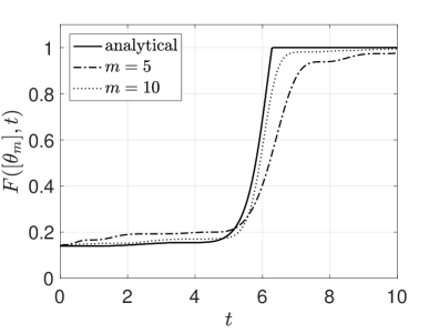
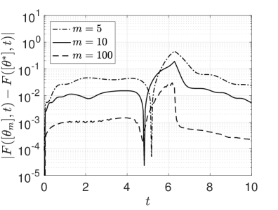
Figure 34: Functional convergence with the number of dimensions $m$. We set $\theta^{*}$ as in (544) and evaluate $F([\theta_{m}],t)$ and the $L_{\infty}$ error $|F([\theta^{*}],t)-F([\theta_{m}],t)|$ versus time for different $m$, where $\theta_{m}(x)$ is the projection of $\theta^{*}(x)$ in the finite dimensional function space $D_{m}$ spanned by the orthonormal polynomial basis shown in Figure 32. It is seen that $m=10$ yields reasonably accurate results.

Functional Derivatives

The first-order functional derivative of the solution functional (541) is

$$\frac{\delta F([\theta],t)}{\delta\theta(x)}=\begin{cases}\displaystyle-2\theta(x)\exp\left[-\int_{t}^{2\pi}\theta(x)^{2}dx\right]&t\in[0,2\pi],\\ \displaystyle-2\theta(x)&t>2\pi.\end{cases}$$ (545)

Note that the functional derivative at time $t$ evaluated at $\theta(x)$ is simply a rescaled version of $\theta(x)$, where the scaling factor grows from $2\exp\left[\int_{0}^{2\pi}\theta(x)dx\right]$ (at $t=0$) to $2$ (at $t=2\pi$). Such derivative can be expressed in $D_{m}$ as

$$\left.\frac{\delta F([\theta],t)}{\delta\theta(x)}\right|_{D_{m}}=\sum_{j=1}^{m}\frac{\partial f}{\partial a_{j}}\varphi_{j}(x),$$ (546)

where

$$f(a_{1},...,a_{m},t)=\prod_{j=1}^{m}\exp\left[-\left(\sum_{k=1}^{m}Z_{jk}(t)a_{k}\right)^{2}\right].$$ (547)

More explicitly,

$$\left.\frac{\delta F([\theta],t)}{\delta\theta(x)}\right|_{D_{m}}=-2f(a_{1},...,a_{m},t)\sum_{p=1}^{m}\varphi_{p}(x)\sum_{k,j=1}^{m}Z_{jp}(t)Z_{jk}(t)a_{k}.$$ (548)

In Figure 35 we plot the analytical solution (540) in two dimensions.

$t=0$                                   $t=1$                                   $t=3$                                   $t=6$

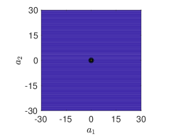
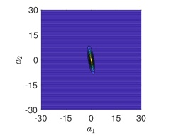
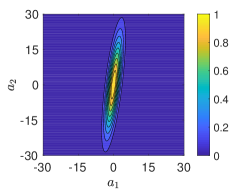
Figure 35: Solution to the multivariate PDE (509) (with $h=0$) in $m=2$ dimensions. The stable spiral at the origin of the characteristic system attracts every curve in the space of modes and ultimately yields $f=1$ everywhere after a transient (see also Figure 34).

The side length of the hypercube cube that encloses any level set of the solution at time $t$ depends on the number of dimensions $m$. In particular, if we are interested in estimating the size of the hypercube that encloses the set $\{\bm{a}\in\mathbb{R}^{m}\,|\,f(\bm{a},t)\geq\epsilon\}$, then we can use the formula

$$\frac{1}{2}\sqrt{\frac{-\log(\epsilon)}{m\lambda_{min}}}\leq b\leq\frac{1}{2}\sqrt{\frac{-\log(\epsilon)}{\lambda_{min}}}.$$ (554)

where $\lambda_{min}$ is the smallest eigenvalue of the matrix $\bm{Z}(t)^{T}\bm{Z}(t)$ (see Equation (517)). In Figure 36 we plot the upper and the lower bound estimates of half of the side length of the hypercube that encloses the $10^{-10}$ level set of the solution at $t=1$ versus the number of dimensions $m$. It is seen that the size of the hypercube increases exponentially fast with $m$. This has important consequences when it comes to numerical simulations. In particular, if we perform simulations with far field boundary conditions, then the size of the computational domain should be chosen large enough to accommodate the support of the solution throughout the simulation time interval of interest.

  $t=1$                                                              $t=3$

Figure 36: Upper and lower bound estimates (554) of the half side length of the hypercube that encloses the $10^{-10}$ level set of the solution at $t=1$ and $t=3$ versus the number of dimensions $m$. It is seen that $b$ increases exponentially fast with $m$. The computational domain should be at least as big as $[-b,b]^{m}$, where $b$ is the number given by the upper curve. For example, if we are aiming at resolving the numerical solution in the case $m=6$ within the time interval $[0,3]$, then we should consider the computational domain $[-b,b]^{6}$ with $b\simeq 1600$.

7.2 Numerical Discretization

Consider the multivariate PDE (509) with $h=0$, hereafter written in the operator form

$$\frac{\partial f}{\partial t}=Lf,$$ (555)

where

$$L=-\sum_{j,k=1}^{m}a_{k}C_{jk}\frac{\partial}{\partial a_{j}}.$$ (556)

Note that $L$ is a separable linear operator with separation rank $r_{L}=m^{2}$. In fact, $L$ can be written in the form

$$L=\sum_{q=1}^{m^{2}}\alpha_{q}L^{q}_{1}(a_{1})\cdots L_{m}^{q}(a_{m}),$$ (557)

for suitable one-dimensional linear operators $L^{q}_{j}(a_{j})$ defined in Table 6.

$q$	$\alpha_{q}$	$L_{1}^{q}$	$L_{2}^{q}$	$\cdots$	$L_{m}^{q}$
$1$	$-C_{11}$	$a_{1}\partial_{a_{1}}$	$1$	$\cdots$	$1$
$2$	$-C_{12}$	$\partial_{a_{1}}$	$a_{2}$	$\cdots$	$1$
$\vdots$	$\vdots$	$\vdots$	$\vdots$	$\vdots$	$\vdots$
$m$	$-C_{1m}$	$\partial_{a_{1}}$	$1$	$\cdots$	$a_{m}$
$m+1$	$-C_{21}$	$a_{1}$	$\partial_{a_{2}}$	$\cdots$	$1$
$m+2$	$-C_{22}$	$1$	$a_{2}\partial_{a_{2}}$	$\cdots$	$1$
$\vdots$	$\vdots$	$\vdots$	$\vdots$	$\vdots$	$\vdots$
$2m$	$-C_{2m}$	$1$	$\partial_{a_{2}}$	$\cdots$	$a_{m}$
$\vdots$	$\vdots$	$\vdots$	$\vdots$	$\vdots$	$\vdots$
$m^{2}-m+1$	$-C_{m1}$	$a_{1}$	$1$	$\cdots$	$\partial_{a_{m}}$
$m^{2}-m+2$	$-C_{m2}$	$1$	$a_{2}$	$\cdots$	$\partial_{a_{m}}$
$\vdots$	$\vdots$	$\vdots$	$\vdots$	$\vdots$	$\vdots$
$m^{2}$	$-C_{mm}$	$1$	$1$	$\cdots$	$a_{m}\partial_{a_{m}}$

Table 6: Ordering of the linear operators defined in equation (557).

The solution to the multivariate PDE (555) can be represented by using any tensor series expansion. In particular, hereafter we consider the hierarchical Tucker format (Section 3.3.1) and the canonical polyadic tensor decomposition (Section 7.2.2).

7.2.1 HT and CP Algorithms with Explicit Time Stepping

Let us discretize the PDE (555) in time by using any explicit time stepping scheme, for example the second-order Adams-Bashforth scheme (see Section 5.2)

$$f_{n+2}=f_{n+1}+\frac{\Delta t}{2}L\left(3f_{n+1}-f_{n}\right).$$ (558)

In this setting, we see that the only operations needed to compute $f_{n+2}$ with tensor methods are: i) addition, ii) application of a (separable) linear operator, and iii) rank reduction, the last operation being the most important among all three. From a computational viewpoint, it would be also very useful if we could split the tensor operations yielding $f_{n+2}$ into sequences of tensor operations followed by rank reduction. In this way we could minimize the storage requirements and the overall computational cost. For example, we could split (558) as

1. Compute a low rank representation of $w_{n+1}=(3f_{n+1}-f_{n})$,

2. Compute a low rank representation of $q_{n+1}=Lw_{n+1}$,

3. Compute a low rank representation of $f_{n+2}=f_{n+1}+\Delta tq_{n+1}/2$.

Are we allowed to do so? Unfortunately no. Splitting tensor operations into sequences of tensor operations followed by rank reduction usually yields severe cancellation errors. In some cases, this problem can be overcome. For example, an efficient and robust algorithm that allows us to split sums and rank reduction operations was recently proposed in [114] in the context of hierarchical Tucker formats. The algorithm leverages on the block diagonal structure that arises when adding hierarchical Tucker format. Also, the vector resulting from application of the separable linear operator $L$ to the hierarchical Tucker format $w_{n+1}$ at point ii) above can be computed very efficiently if we have available a hierarchical Tucker representation of the operator $L$. Such representation can be easily constructed in a Fourier collocation setting by vectorizing all operators in table 6. Each one-dimensional operator is represented relative to a basis trigonometric (nodal) polynomials (Fourier spectral collocation method) [84] In practice, we simply need to convert the vectorized canonical polyadic series of $L$ into a hierarchical Tucker expansion, which is a relative standard operation.

7.2.2 CP-ALS Algorithm with Implicit Time Stepping

Let us discretize the PDE (555) in time by using the Crank-Nicolson method. This yields

$$\left[I-\frac{\Delta t}{2}L\right]f_{n+1}=\left[I+\frac{\Delta t}{2}L\right]f_{n}.$$ (559)

This equation can be written in a compact notation as

$$Af_{n+1}=Bf_{n},$$ (560)

where

$$A=I-\frac{\Delta t}{2}L,\quad\textrm{and}\quad B=I+\frac{\Delta t}{2}L.$$ (561)

By using the definition of $L$ given in (557) (see also Table 6), it is clear that both $A$ and $B$ are separable operators in the form

$$A=1\cdots 1+\frac{\Delta t}{2}\sum_{i,j=1}^{m}a_{i}C_{ji}\frac{\partial}{\partial a_{j}},$$ (562)

$$B=1\cdots 1-\frac{\Delta t}{2}\sum_{i,j=1}^{m}a_{i}C_{ji}\frac{\partial}{\partial a_{j}}.$$ (563)

These operators have separation rank $r_{A}=r_{B}=m^{2}+1$ and can be conveniently written as

$$A=\sum_{q=0}^{m^{2}}\eta_{q}E^{q}_{1}(a_{1})\cdots E^{q}_{m}(a_{m}),\qquad B=\sum_{q=0}^{m^{2}}\zeta_{q}E^{q}_{1}(a_{1})\cdots E^{q}_{m}(a_{m}),$$ (564)

where all quantities are defined in Table 7. The difference with Table 6 is that we added one row (the zeroth one) to represent the identity operator $1\cdots 1$, and we rescaled all coefficients $C_{ij}$.

$q$	$\eta_{q}$	$\zeta_{q}$	$E_{1}^{q}$	$E_{2}^{q}$	$\cdots$	$E_{m}^{q}$
$0$	$1$	$1$	$1$	$1$	$\cdots$	$1$
$1$	$\Delta tC_{11}/2$	$-\Delta tC_{11}/2$	$a_{1}\partial_{a_{1}}$	$1$	$\cdots$	$1$
$2$	$\Delta tC_{12}/2$	$-\Delta tC_{12}/2$	$\partial_{a_{1}}$	$a_{2}$	$\cdots$	$1$
$\vdots$	$\vdots$	$\vdots$	$\vdots$	$\vdots$	$\vdots$
$m$	$\Delta tC_{1m}/2$	$-\Delta tC_{1m}/2$	$\partial_{a_{1}}$	$1$	$\cdots$	$a_{m}$
$m+1$	$\Delta tC_{21}/2$	$-\Delta tC_{21}/2$	$a_{1}$	$\partial_{a_{2}}$	$\cdots$	$1$
$m+2$	$\Delta tC_{22}/2$	$-\Delta tC_{22}/2$	$1$	$a_{2}\partial_{a_{2}}$	$\cdots$	$1$
$\vdots$	$\vdots$	$\vdots$	$\vdots$	$\vdots$	$\vdots$
$2m$	$\Delta tC_{2m}/2$	$-\Delta tC_{2m}/2$	$1$	$\partial_{a_{2}}$	$\cdots$	$a_{m}$
$\vdots$	$\vdots$	$\vdots$	$\vdots$	$\vdots$	$\vdots$
$m^{2}-m+1$	$\Delta tC_{m1}/2$	$-\Delta tC_{m1}/2$	$a_{1}$	$1$	$\cdots$	$\partial_{a_{m}}$
$m^{2}-m+2$	$\Delta tC_{m2}/2$	$-\Delta tC_{m2}/2$	$1$	$a_{2}$	$\cdots$	$\partial_{a_{m}}$
$\vdots$	$\vdots$	$\vdots$	$\vdots$	$\vdots$	$\vdots$
$m^{2}$	$\Delta tC_{mm}/2$	$-\Delta tC_{mm}/2$	$1$	$1$	$\cdots$	$a_{m}\partial_{a_{m}}$

Table 7: Ordering of the linear operators $A$ and $B$ defined in (564).

A substitution of the CP decomposition

$$\hat{f}_{n+1}=\sum_{l=1}^{r}\prod_{k=1}^{m}{G^{l}_{k}(a_{k},t_{n+1})}$$ (565)

into equation (559) yields the residual

$$R=A\hat{f}_{n+1}-B\hat{f}_{n}.$$ (566)

Minimization of the $L_{2}$ norm of (566) with respect to ${\bm{\beta}}_{q}(t_{n+1})$ yields the linear systems of equations

$$\bm{M}^{L}_{q}\bm{\beta}_{q}(t_{n+1})=\bm{M}^{R}_{q}\bm{\beta}_{q}(t_{n}),\qquad q=1,...,m$$ (567)

where

$$\bm{M}^{L}_{q}=\sum_{e,z=0}^{m^{2}}K^{L}_{ez}\left[{\displaystyle\begin{subarray}{c}\vspace{0.2cm}\\ \vspace{0.04cm}m\\ \bigcirc\\ k=1\\ k\neq q\end{subarray}}\hat{\bm{\beta}}_{k}(t_{n+1})^{T}\bm{E}^{ez}_{k}\hat{\bm{\beta}}_{k}(t_{n+1})\right]^{T}\otimes\left[{\bm{E}}^{ez}_{q}\right]^{T},$$ (568)

$$\bm{M}^{R}_{q}=\sum_{e,z=0}^{m^{2}}{K}^{R}_{ez}\left[{\begin{subarray}{c}\vspace{0.2cm}\\ \vspace{0.04cm}m\\ \bigcirc\\ k=1\\ k\neq q\end{subarray}}\hat{\bm{\beta}}_{k}(t_{n})^{T}{\bm{E}}^{ez}_{k}\hat{\bm{\beta}}_{k}(t_{n+1})\right]^{T}\otimes\left[{\bm{E}}^{ez}_{q}\right]^{T},$$ (569)

and

$$\left[{\bm{E}}^{ez}_{q}\right]_{sh}=\int_{-b}^{b}E_{q}^{e}(a)\phi_{s}(a)E_{q}^{z}(a)\phi_{h}(a)da.$$ (570)

In equations (568)-(569), $\bigcirc$ denotes the Hadamard matrix product, $\otimes$ is the Kroneker matrix product, $\hat{\bm{\beta}}_{k}$ is the matrix version of $\bm{\beta}_{k}$, i.e.,

$$\hat{\bm{\beta}}_{k}(t_{n})=\left[\begin{array}[]{ccc}\beta^{1}_{k1}(t_{n})&\cdots&\beta^{r}_{k1}(t_{n})\\ \vdots&\ddots&\vdots\\ \beta^{1}_{kQ}(t_{n})&\cdots&\beta^{r}_{kQ}(t_{n})\end{array}\right],$$ (571)

$\bm{E}^{ez}_{q}$ is the $Q\times Q$ matrix (570), and $K^{L}_{ez}$ and ${K}^{R}_{ez}$ are entries of the matrices

$$\bm{K}^{L}=\bm{\eta}\bm{\eta}^{T},\quad\textrm{and}\quad\bm{K}^{R}=\bm{\eta}\bm{\zeta}^{T},$$ (572)

where $\bm{\eta}$ and $\bm{\zeta}$ are column vectors with entries $\eta_{q}$ and $\zeta_{q}$ defined in Table 7.

Computing the Matrix System

There are many of symmetries we can exploit when constructing the separated series expansion of the operators $A$ and $B$ in (564). Indeed, a closer look at Table 7 suggests that if we employ the same series expansion in each variable $a_{j}$ (e.g., a trigonometric series) then the number of operators in (564) that we effectively need to compute reduces to the following four

$$1,\qquad a_{j},\qquad\frac{\partial}{\partial a_{j}},\qquad a_{j}\frac{\partial}{\partial a_{j}}.$$ (573)

This means that the number of terms that are effectively different in the fundamental matrix (570) are only 12 (9 if we are willing to employ matrix transposes). Specifically,

$$\begin{array}[]{l l l l}\displaystyle 1.\,\int_{-b}^{b}\phi_{s}\phi_{h}da&\displaystyle 2.\,\int_{-b}^{b}a\phi_{s}\phi_{h}da,&\displaystyle 3.\,\int_{-b}^{b}\phi_{s}\frac{d\phi_{h}}{da}da,&\displaystyle 4.\,\int_{-b}^{b}a\phi_{s}\frac{d\phi_{h}}{da}da,\\ \displaystyle 5.\,\int_{-b}^{b}a^{2}\phi_{s}\phi_{h}da,&\displaystyle 6\,\int_{-b}^{b}a^{2}\phi_{s}\frac{d\phi_{h}}{da}da,&\displaystyle 7.\,\int_{-b}^{b}\frac{d\phi_{s}}{da}\phi_{h}da,&\displaystyle 8.\,\int_{-b}^{b}a\frac{d\phi_{s}}{da}\phi_{h}da,\\ \displaystyle 9.\,\int_{-b}^{b}\frac{d\phi_{s}}{da}\frac{d\phi_{h}}{da}da,&\displaystyle 10.\,\int_{-b}^{b}a\frac{d\phi_{s}}{da}\frac{d\phi_{h}}{da}da,&\displaystyle 11.\,\int_{-b}^{b}a^{2}\frac{d\phi_{s}}{da}\phi_{h}da,&\displaystyle 12.\,\int_{-b}^{b}a^{2}\frac{d\phi_{s}}{da}\frac{d\phi_{h}}{da}da.\end{array}$$ (574)

All these integrals can be pre-computed and stored as $Q\times Q$ matrices (see Eq. (420)). For each $e$, $z$ and $q$, the tensor (570) corresponds to one of the $12$ integrals above. Such map, denoted as $g^{ez}_{q}$, takes in the triple $(e,z,q)$, where $q\in\{1,...,m\}$ and $e,z\in\{0,...,m^{2}\}$, and it returns a number between $1$ and $12$ identifying which integral in the set (557) corresponds to the tensor entry in (570). For example, if we sort the operators as in Table 7 then in $m=2$ dimensions we have

$$g^{ez}_{1}=\left[\begin{array}[]{ccccc}1&8&7&2&1\\ 4&12&10&6&4\\ 3&10&9&4&3\\ 2&11&8&5&2\\ 1&8&7&2&1\end{array}\right]\qquad\qquad g^{ez}_{2}=\left[\begin{array}[]{c c c c c}1&1&2&7&8\\ 1&1&2&7&8\\ 2&2&5&8&11\\ 3&3&4&9&10\\ 4&4&6&10&12\end{array}\right],$$ (575)

while in dimension $m=3$ we have, e.g.,

$$g^{ez}_{1}=\left[\begin{array}[]{cccccccccc}1&8&7&7&2&1&1&2&1&1\\ 4&12&10&10&6&4&4&6&4&4\\ 3&10&9&9&4&3&3&4&3&3\\ 3&10&9&9&4&3&3&4&3&3\\ 2&11&8&8&5&2&2&5&2&2\\ 1&8&7&7&2&1&1&2&1&1\\ 1&8&7&7&2&1&1&2&1&1\\ 2&11&8&8&5&2&2&5&2&2\\ 1&8&7&7&2&1&1&2&1&1\\ 1&8&7&7&2&1&1&2&1&1\end{array}\right].$$ (576)

A combinatorial argument shows that the number of entries equal to $1$, $2$, $3$, etc., in each matrix $g_{1}^{ez}$, $g_{2}^{ez}$, …, $g_{m}^{ez}$ is the same (for fixed $m$). For instance, in (575) we have $4$ ones, $2$ threes, $3$ fours, $1$ five, etc. This is very useful when we break the sum in $e$ and $z$ in (568) and (569) into multiple sums, and use the associative property of the tensor product to reduce the number of operations. By using the map $g_{q}^{ez}$ we can immediately identify each matrix $\bm{E}_{q}^{ez}$. For example, in the case $m=2$ we have (see Eq. (575))

$$\left[{\bm{E}}^{11}_{1}\right]_{sh}=\int_{-b}^{b}\phi_{s}(a)\phi_{h}(a)da,\qquad\left[{\bm{E}}^{12}_{1}\right]_{sh}=\int_{-b}^{b}a\frac{d\phi_{s}(a)}{da}\phi_{h}(a)da,\quad...\quad.$$ (577)

Summary of the Algorithm

We first compute all integrals in (574) and store them in $12$ matrices $Q\times Q$, $Q$ being the number of degrees of freedom in each variable (e.g., collocation points of Fourier modes). We also set up the map between such set of matrices and any element of the tensor (570). Such map basically takes in the triple $(q,e,z)$, where $q\in\{1,...,m\}$ and $e,z\in\{0,...,m^{2}\}$, and it returns a number between $1$ and $12$ identifying which integral in the set (557) corresponds to the tensor entry in (570). In a matrix setting, this basically allows us to efficiently compute each matrix $\bm{E}_{q}^{ez}$ appearing in (568) and (569). Next, we compute the compute the canonical tensor decomposition of the initial condition $f_{0}(a_{1},...,a_{m})$, by applying the methods we described in Section 3.3.1. This gives us the set of vectors $\{\bm{\beta}_{1}(t_{0}),...,\bm{\beta}_{m}(t_{0})\}$. With such vectors available, we can build the matrices $\bm{M}^{L}_{1}$ and $\bm{M}^{R}_{1}$ defined in (568) and (569). To this end, we need an initial guess for $\{\bm{\beta}_{1}(t_{1}),...,\bm{\beta}_{m}(t_{1})\}$ which we can take to be equal to $\{\bm{\beta}_{1}(t_{0}),...,\bm{\beta}_{m}(t_{0})\}$, or a small random perturbation of it. With $\bm{M}^{L}_{1}$ and $\bm{M}^{R}_{1}$ in place and set, we can solve the linear system (567) and update $\bm{\beta}_{1}(t_{1})$. At this point we recompute $\bm{M}^{L}_{2}$ and $\bm{M}^{R}_{2}$ (with the updated $\bm{\beta}_{1}(t_{1})$) and solve for $\bm{\beta}_{2}(t_{1})$. We repeat this process for $q=3,...,m$ and iterate over and over among all variables until convergence. Parallel versions of the ALS algorithm were recently proposed by Karlsson et al. in [100].

7.2.3 Long-Term Integration

A rigorous error analysis of the HT and CP-ALS algorithms to solve the multivariate PDE (555) goes beyond the scope of this report (see [8] for a recent account). It it useful, however, to point out a few things on the nature of the discretization error, in particular on how the temporal local truncation error depends on the dimension $m$. To this end, let us first recall that the local truncation error at time $t_{n+1}$ of the second-order Adams Bashforth (AB2) scheme applied to the linear PDE (555) is $5\Delta t^{3}L^{3}f(\eta,\bm{a})/12$, where $\eta$ is some time instant between $t_{n}$ and $t_{n+1}$, $f(\eta,\bm{a})$ is the exact solution (515), and $L$ is defined in (556). The operator $L^{2}$ can be explicitly written as

$$L^{2}= \sum_{i,j,l,p=1}^{m}x_{l}C_{pl}\frac{\partial}{\partial a_{p}}\left(x_{j}C_{ij}\frac{\partial}{\partial a_{j}}\right)$$

$$= \sum_{i,j,l,p=1}^{m}x_{l}C_{pl}C_{ij}\left(\delta_{jp}\frac{\partial}{\partial a_{j}}+x_{j}\frac{\partial^{2}}{\partial a_{j}\partial a_{p}}\right),$$ (578)

while $L^{3}$ has the form

$$L^{3}= \sum_{i,j,l,p,q,z=1}^{m}x_{q}C_{zq}C_{pl}C_{ij}\delta_{lq}\left(\delta_{jp}\frac{\partial}{\partial a_{j}}+x_{j}\frac{\partial^{2}}{\partial a_{j}\partial a_{p}}\right)+$$

$$\sum_{i,j,l,p,q,z=1}^{m}x_{q}x_{l}C_{zq}C_{pl}C_{ij}\left(\delta_{jp}\frac{\partial^{2}}{\partial a_{j}\partial a_{z}}+\delta_{jz}\frac{\partial^{2}}{\partial a_{j}\partial a_{p}}+x_{j}\frac{\partial^{3}}{\partial a_{j}\partial a_{p}\partial a_{z}}\right).$$ (579)

From the last expression it is clear that any inaccuracy in the computation of the derivatives adds up to the temporal truncation error with at least with factor $m^{6}$. Indeed, as shown in Figure 37, the norm of $L^{3}f$ grows faster than $m^{6}$. This has important consequences on the accuracy attainable with the AB2 time-integration scheme applied to high-dimensional linear PDEs.

Figure 37: Norm of $L^{3}f$ at initial time versus $m$. The operator $L^{3}$, defined (579), has been discretized in space by using an accurate Fourier spectral method with $N=600$ points in each dimension. It is seen that the norm of $L^{3}f_{0}$ grows faster than $m^{6}$. This has important consequences on the local truncation error generated by AB2 time-integrator applied to the PDF (555).

In fact, suppose that $\left\|L^{3}f\right\|$ grows like $m^{6}$ not just at initial time but at each time step (it actually grows faster than that), i.e.,

$$\left\|L^{3}f\right\|\sim\kappa m^{6},$$ (580)

where $\kappa$ is a suitable constant. If we want the AB2 scheme to operate at constant truncation error for different number of dimensions $m$ then we need to guarantee that

$$m_{1}^{6}\Delta t_{1}^{3}=m_{2}^{6}\Delta t_{2}^{3}.$$ (581)

For example, if $m_{1}=2$ and $m_{2}=10$ then we have

$$\Delta t_{2}=\frac{\Delta t_{1}}{25}.$$ (582)

In other words, if we want our time integrator to operate at constant truncation error, then we need to run the simulation in $10$ dimensions with a time step that is roughly $25$ times smaller than the one we emply in the simulation in $2$ dimensions. This can tax the computational resources quite substantially. In fact, suppose we are interested in integrating our PDE up to $T=1$, and we set $\Delta t_{1}=10^{-4}$ in $2$ dimensions, i.e., $10^{4}$ time steps. Assuming that the local truncation error is the same at each time step (see Eq. (580)), at the end of the integration period we accumulated an error of approximately $10^{-6}\kappa$. The same error is roughly attained at $T=0.04$ if we integrate the PDE in $10$ dimensions. In fact, the time step $\Delta t_{2}=\Delta t_{1}/25$ guarantees a constant local truncation error which adds up to $10^{-6}\kappa$ after just $0.04$ time units. The local truncation error manifest itself as numerical diffusion which eventually dissipates the numerical solution to zero. Note that in this simple calculation we did not take into account the accuracy of the rank reduction process in the CP-ALS and HT algorithms, which takes place at each time step.

7.3 Numerical Results

We solve the multivariate PDE (555) in the hypercube $[-b,b]^{m}$, with $b=60$ and variable $m$. Such domain is chosen large enough to accommodate periodic (zero) boundary conditions in the integration period of interest. We study both the HT (hierarchical Tucker) and the CP-ALS schemes we discussed in Section 7.2.1 and Section 7.2.2. Specifically, we implemented a Fourier collocation method with $600$ nodes in each variable and explicit AB2 time stepping. To study the accuracy of the numerical solution, we consider the time-dependent relative error

$$\epsilon_{m}(t)=\left|\frac{F([\theta_{m}^{*}],t)-\hat{F}([\theta_{m}^{*}],t)}{F([\theta_{m}^{*}],t)}\right|,$$ (583)

where $F$ is the analytical solution (540), $\hat{F}$ is the numerical solution we obtained by using the CP-ALS or the HT algorithms in the test function space $D_{m}$ (i.e., $m$ with independent variables) and with separation rank $r$. The test function $\theta^{*}$ in (583) is defined as

$$\theta_{m}^{*}(x)=h\sum_{j=1}^{m}\varphi_{j}(x),\qquad h=0.698835274542439,$$ (584)

where $\varphi_{j}(x)$ are the orthonormal polynomials shown in Figure 32. The accuracy of the CP-ALS and the HT algorithms is studied in Figure 38, where we plot the relative pointwise error (583) for different separation ranks $r$ and for different number of dimensions. It is seen that, as expected, the accuracy of the numerical solution increases as we increase the separation rank. Also, as we increase the number of dimensions from $2$ to $6$ the relative error increases, in agreement with the results of Section 7.2.3 (we emply a constant $\Delta t=2.55\times 10^{-4}$ in all our simulations). It is worthwhile emphasizing that the CP-ALS is a randomized algorithm which requires initialization at each time-step. This means that results of simulations with the same nominal parameters may be different. On the other hand, tensor methods based on multivariate/distributed singular value decomposition, such as the hierarchical Tucker decomposition [77], do not suffer from this issue. The CP-ALS algorithm is faster than HT but, as we just said, accuracy control may be an issue. The separation rank of both the CP-ALS and HT algorithms are computed adaptively up to the maximum value $r_{max}$ specified in the legend of Figure 38.

     CP-ALS                                                         HT

two dimensions   

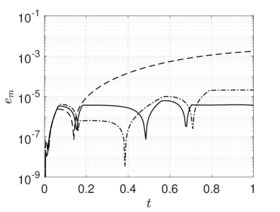
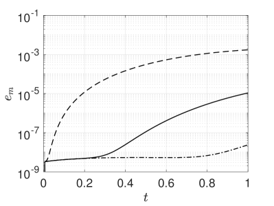
three dimensions   

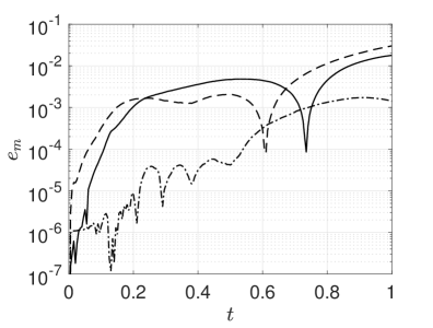
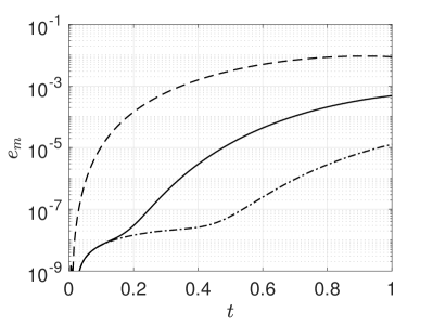
six dimensions   

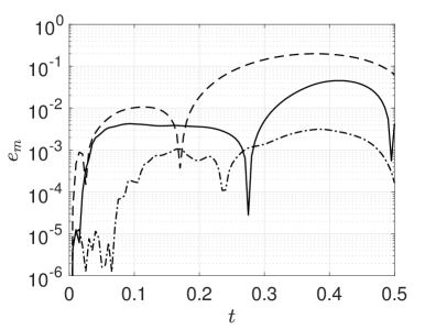
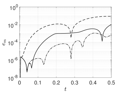
$--$ $r_{max}=4$          — $r_{max}=8$           $-\cdot-$ $r_{max}=12$

Figure 38: Accuracy of the numerical solution to the FDE (504) in the finite dimensional function space (539) for different number of dimensions. Specifically, we plot the relative $L_{\infty}$ error (583) versus time we obtained by using the CP-ALS and HT algorithms we discussed in Section 7.2. The separation rank of both CP-ALS and HT is computed adaptively at each time step up to the maximum value $r_{max}$.

Note that in two dimensions the CP-ALS algorithm results in error plots that looks very similar when $r_{max}=8$ and $r_{max}=12$. This is because the separation rank is less than $8$ in both cases throughout the simulation up to $t=1$. The variability of the results is related to the random initialization required by the ALS algorithm at each time step. On the other hand, in three and six dimensions the error plots we obtain for $r_{m}ax=4$ and $r_{m}ax=8$ are of the same order of magnitude because such separation ranks are achieved after just few time steps and they are not sufficient to accurately represent the multivariate solution. A similar phenomenon attributable to the separation rank is observed in the HT simulations. In particular, the time instant at which the HT tensor series requires a separation rank higher than $8$ can be clearly identified, i.e., at $t=0.2$ in two dimensions, at $t=0.1$ in three dimensions, and at $t=0.05$ in six dimensions. In Figure 39 we plot the time evolution of the first three CP modes $G_{6}^{1}$, $G_{6}^{2}$ and $G_{6}^{3}$ (see equation (565)) representing the dynamics of the solution functional in the variable $a_{6}=(\theta,\varphi_{6})$.

$t=0.01$       

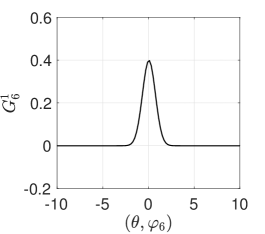
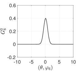
$t=0.5$       

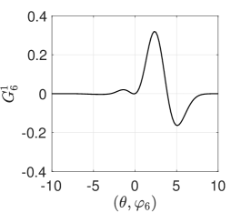
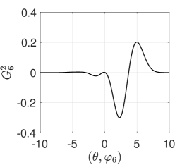
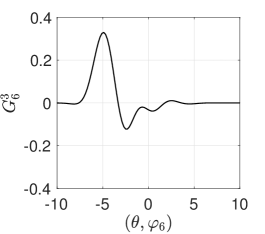
Figure 39: Time evolution of the first three CP modes representing the dynamics along $a_{6}=(\theta,\varphi_{6})$ in the CP expansion (565) of the solution functional. These modes are obtained by solving numerically the FDE (504) in the function space $D_{6}$ (see Eq. (539)) with the CP-ALS algorithm.

Remark: If $\theta(x)$ is not in the function space $D_{m}$ (see Eq. (539)), but can be represented in $D_{m}$ with accuracy then the solution to the multivariate PDE (555) provides an approximation of the solution to the full FDE (504) at such $\theta(x)$. For instance, consider the following test function

$$\theta(x)=\sin(x).$$ (585)

The Fourier coefficients of $\theta$ relative to the orthonormal basis shown in Figure 32 are plotted in Figure (40). Clearly $\theta(x)$ is not in $D_{6}$, but it can be approximated well in $D_{6}$. This means that the solution to the FDE at $\sin(x)$ can be approximated by the solution of the six-dimensional PDE arising when we evaluate the FDE (504) $D_{6}$.

(a)                                                              (b)

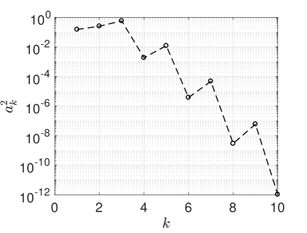
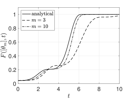
Figure 40: (a) Fourier coefficients of $\sin(x)$ relative to the orthonormal polynomial basis shown in Figure 32. (b) Comparison between the solution to the FDE in $D_{3}$ and $D_{10}$ and the exact solution (541) evaluated at $\theta(x)=\sin(x)$.

Computing Functional Derivatives

In Figure 41 we compare the exact first-order functional derivative (545) at $t=0.4$ with the numerical approximation we obtained with the HT algorithm in $m=3$ and $m=6$ dimensions. The separation rank of the tensor series expansions is set to $r=12$. As expected, the numerical approximation converges to the exact solution as we increase the number of dimensions.

      $\theta(x)=\sin(x)$                                               $\theta(x)=xe^{-x^{2}/4}$

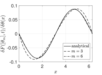
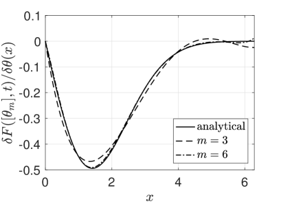
Figure 41: First-order functional derivative of the solution functional (541) at $t=0.4$, evaluated at the test functions $\theta(x)=\sin(x)$ and $\theta(x)=xe^{-x^{2}/4}$. We plot the exact result (545) and the numerical approximation (548) we obtained in the function spaces $D_{3}$ and $D_{6}$ (see Eq. (539)). The numerical approximation is computed by solving the mutivariate PDE (509) in three and six dimensions.

7.4 The Navier-Stokes-Hopf Functional Equation

In this Section we discuss approximation of the Navier-Stokes-Hopf functional equation

$$\frac{\partial\Phi([\bm{\theta}],t)}{\partial t}=\sum_{k=1}^{3}\int_{V}\theta_{k}(\bm{x})\left[i\sum_{j=1}^{3}\frac{\partial}{\partial x_{j}}\left(\frac{\delta^{2}\Phi([\bm{\theta}],t)}{\delta\theta_{k}(\bm{x})\delta\theta_{j}(\bm{x})}\right)+\nu\nabla^{2}\left(\frac{\delta\Phi([\bm{\theta}],t)}{\delta\theta_{k}(\bm{x})}\right)\right]d\bm{x}.$$ (586)

In this formulation, $V$ is a periodic box and $\bm{\theta}(\bm{x})$ is chosen in a divergence-free space of test functions. The main advantage of using such divergence-free space is that the pressure term drops out, just as in the classical Navier-Stokes equations. To develop a discretization of the Hopf equation (586) it is convenient to first address the question of how to represent divergence-free spaces of periodic functions in 2D and 3D.

7.4.1 Symmetries of the Solution Functional

The divergence-free constraint in the velocity field induces a certain number of symmetries in the Hopf functional. Let first assume that the flow develops in a bounded region $V$, i.e., $\bm{u}\cdot\widehat{\bm{n}}=0$, where $\widehat{\bm{n}}$ is the outward unit vector normal to the boundary of $V$. Such region could be any volume co-moving with the fluid. In this assumption,

$$\Phi([\bm{\theta}+\nabla\varphi])=\Phi([\bm{\theta}])$$ (590)

for any $\bm{\theta}(\bm{x})$ and any $\varphi(\bm{x})$. In fact,

$$\int_{V}\bm{u}\cdot\nabla\varphi d\bm{x}=\int_{\partial V}\varphi\bm{u}\cdot\hat{\bm{n}}d\bm{x}=0.$$ (591)

If the boundary conditions assigned to $\bm{u}$ on $\partial V$ (boundary of $V$) are different from $\bm{u}\cdot\hat{\bm{n}}=0$, then (590) is still valid, but not for any $\varphi(\bm{x})$. For example, if $\bm{u}$ is not orthogonal to $\hat{\bm{n}}$ along some part of the boundary $\partial V$, then it is sufficient to set $\varphi=0$ along such boundary and use the fact that $\nabla\cdot\bm{u}=0$ to conclude that (590) is still valid. Now let us consider the Helmholtz decomposition

$$\bm{\theta}=\bm{\eta}+\nabla\varphi,$$ (592)

where $\nabla\cdot\bm{\eta}=0$ in the domain $V$, and $\varphi=0$ at the boundary $\partial V$. By taking the divergence of (592) we conclude that $\varphi$ satisfies the Dirichlet boundary value problem

$$\nabla^{2}\varphi=\nabla\cdot\bm{\theta}\quad\textrm{(in $V$)},\qquad\varphi=0\quad\textrm{(in $\partial V$)},$$ (593)

which has a solution. With the decomposition (592) available, we have

$$\Phi([\bm{\eta}+\nabla\varphi])=\Phi([\bm{\eta}]).$$ (594)

In fact,

$$\int_{V}(\bm{\eta}+\nabla\varphi)\cdot\bm{u}d\bm{x}=\int_{V}\bm{\eta}\cdot\bm{u}d\bm{x}+\int_{V}\nabla\varphi\cdot\bm{u}d\bm{x}.$$ (595)

However, by applying the Gauss theorem (recall that $\nabla\cdot\bm{u}=0$)

$$\int_{V}\nabla\varphi\cdot\bm{u}dV=\int_{\partial V}\varphi\bm{u}\cdot\widehat{\bm{n}}d\bm{x}=0$$ (596)

Therefore (594) holds. The boundary conditions for $\bm{\eta}=\bm{\theta}-\nabla\varphi$ depend on the gradient of the solution to (593) at the boundary $\partial V$. Next, consider the unique Helmholtz-Hodge decomposition (see [20] or [34], p. 36) of the field $\bm{\theta}$ in the form (592), where $\nabla\cdot\bm{\eta}=0$ and $\bm{\eta}$ is tangent to $\partial V$, i.e., $\bm{\eta}\cdot\hat{\bm{n}}=0$ ($\hat{\bm{n}}$ outward unit vector normal to $\partial V$). If there is no flow across the boundary $\partial V$ ($\bm{u}\cdot\hat{\bm{n}}=0$), or if the boundary conditions of $\varphi$ are chosen such that the integral at the right hand side of (596) is zero then we have the symmetry (594). For example, if $\varphi$ is constant along the boundary then the divergence-free requirement on $\bm{u}$ implies that the integral at the right hand side of (596) is zero. Also, if $\bm{\theta}$ and $\bm{u}$ are periodic on a box then $\varphi$ is periodic and the boundary integral in (596) is zero. In fact, the field $\varphi$ arising from the Helmoltz-Hodge decomposition of $\bm{\theta}$ is the unique solution to the Neuman problem (see [34], p. 36)

$$\nabla^{2}\varphi=\nabla\cdot\bm{\theta}\quad\textrm{(in $V$)},\qquad\frac{\partial\varphi}{\partial n}=\bm{\theta}\cdot\widehat{\bm{n}}\quad\textrm{(in $\partial V$)}.$$ (597)

Clearly, if $\bm{\theta}$ is periodic then $\varphi$ is periodic and therefore $\bm{\eta}$ is periodic too. In other words, If we evaluate $\Phi$ on a space of periodic functions then we have the invariance

$$\Phi([\bm{\theta}])=\Phi([\bm{\eta}]),$$ (598)

where $\bm{\eta}$ is periodic and divergence free ($\bm{\eta}$ is the divergence-free part arising from the unique Helmholtz-Hodge decomposition of $\bm{\theta}$.

7.4.2 Divergence-Free Function Spaces

There has been a significant research activity in identifying bases for divergence-free spaces of functions. For example, Deriaz and Perrier [37, 38] have developed an effective algorithm to construct divergence-free and curl-free wavelets in 2D and 3D with various types of boundary conditions. Other divergence-free bases can be constructed in terms of radial basis functions [240], trigonometric polynomials [200], or eigenvalue problems with appropriate boundary conditions conditions [226, 169]. Hereafter we discuss how to construct a divergence-free basis for two-dimensional periodic flows. To this end, we consider the tensor product basis

$$\psi_{n}(x,y)=l_{j(n)}(x)l_{i(n)}(y),$$ (599)

where $j(n)$ and $i(n)$ are suitable sequences of integer number while $l_{k}(x)$ are trigonometric polynomials. Any scalar-valued periodic function on the square (such as the streamfunction) can be represented as

$$\Psi(x,y)=\sum_{k=1}^{M}\alpha_{k}\psi_{j}(x,y).$$ (600)

Next define the divergence-free basis

$$\bm{\Gamma}_{k}(x,y)=\left(\frac{\partial\psi_{k}(x,y)}{\partial y},\,-\frac{\partial\psi_{k}(x,y)}{\partial x}\right).$$ (601)

It is clear that each basis element $\bm{\Gamma}_{k}$ is divergence-free by construction, i.e., $\nabla\cdot\bm{\Gamma}_{k}=0$. However, the basis (601) is not orthogonal nor normalized relative to the $L_{2}([-b,b]^{2})$ inner product

$$\left(\bm{\Gamma}_{i},\bm{\Gamma}_{j}\right)= \int_{-b}^{b}\int_{-b}^{b}\bm{\Gamma}_{i}\cdot\bm{\Gamma}_{j}dxdy,$$

$$= \int_{-b}^{b}\int_{-b}^{b}\left(\frac{\partial\psi_{i}}{\partial y}\frac{\partial\psi_{j}}{\partial y}+\frac{\partial\psi_{i}}{\partial x}\frac{\partial\psi_{j}}{\partial x}\right)dxdy.$$

To generate a divergence-free and orthonormal basis one could use the Gram-Schmidt orthogonalization. As we shall see hereafter, such procedure preserves the divergence-free character of each basis element. We first normalize $\bm{\Gamma}_{1}$ as

$$\widehat{\bm{\Gamma}}_{1}(x,y)=\frac{\bm{\Gamma}_{1}(x,y)}{\left\|\bm{\Gamma}_{1}(x,y)\right\|},\qquad\left\|\bm{\Gamma}_{1}\right\|=\sqrt{(\bm{\Gamma}_{1},\bm{\Gamma}_{1})}.$$ (602)

Clearly, $\nabla\cdot\widehat{\bm{\Gamma}}_{1}=0$ since the $L_{2}$ norm of $\bm{\Gamma}_{1}$ is just a real number. Next, define

$$\bm{\Theta}_{2}=\bm{\Gamma}_{2}-(\bm{\Gamma}_{2},\widehat{\bm{\Gamma}}_{1})\widehat{\bm{\Gamma}}_{1},\qquad\widehat{\bm{\Gamma}}_{2}(x,y)=\frac{\bm{\Theta}_{2}(x,y)}{\left\|\bm{\Theta}_{2}(x,y)\right\|}.$$ (603)

As before, $\nabla\cdot\widehat{\bm{\Gamma}}_{2}=0$. Moreover $\widehat{\bm{\Gamma}}_{2}$ is orthogonal to $\widehat{\bm{\Gamma}}_{1}$, i.e., $(\widehat{\bm{\Gamma}}_{1},\widehat{\bm{\Gamma}}_{2})=0$. The algorithm proceeds with the computation of

$$\bm{\Theta}_{3}=\bm{\Gamma}_{3}-(\bm{\Gamma}_{3},\widehat{\bm{\Gamma}}_{2})\widehat{\bm{\Gamma}}_{2}-(\bm{\Gamma}_{3},\widehat{\bm{\Gamma}}_{1})\widehat{\bm{\Gamma}}_{1},\qquad\widehat{\bm{\Gamma}}_{3}(x,y)=\frac{\bm{\Theta}_{3}(x,y)}{\left\|\bm{\Theta}_{3}(x,y)\right\|}.$$ (604)

Thanks to the fact that $\bm{\Gamma}_{3}$, $\widehat{\bm{\Gamma}}_{2}$ and $\widehat{\bm{\Gamma}}_{1}$ are divergence free, we have that $\nabla\cdot\widehat{\bm{\Gamma}}_{3}=0$. Moreover $\widehat{\bm{\Gamma}}_{3}$ is orthogonal to both $\widehat{\bm{\Gamma}}_{2}$ and $\widehat{\bm{\Gamma}}_{1}$. In other words, $\{\widehat{\bm{\Gamma}}_{1},\widehat{\bm{\Gamma}}_{2},\widehat{\bm{\Gamma}}_{3}\}$ is a divergence-free orthonormal system. Proceeding in a similar way, we can construct the divergence-free orthonormal basis we were looking for, and define the following finite-dimensional divergence-free space of functions

$$D_{M}=\textrm{span}\{\bm{\Gamma}_{1},\cdots,\bm{\Gamma}_{M}\}.$$ (605)

An element of $D_{M}$ is in the form

$$\bm{\theta}(x,y)=\sum_{k=1}^{M}a_{k}\hat{\bm{\Gamma}}_{k}(x,y).$$ (606)

7.4.3 Analytical Solution to the Characteristic Function Equation

A substitution of (606) into the Navier-Stokes-Hopf equation (586) yields the multivariate (complex-valued) PDE

$$\frac{\partial\phi}{\partial t}=i\sum_{p,j,k=1}^{M}A_{pjk}a_{p}\frac{\partial^{2}\phi}{\partial a_{k}\partial a_{j}}+\nu\sum_{k,p=1}^{M}a_{p}B_{pk}\frac{\partial\phi}{\partial a_{k}},$$ (609)

where

$$B_{pk}=\int_{V}\widehat{\bm{\Gamma}}_{p}\cdot\nabla^{2}\widehat{\bm{\Gamma}}_{k}d\bm{x},\qquad A_{pjk}=\int_{V}\widehat{\bm{\Gamma}}_{p}\cdot\left[\left(\widehat{\bm{\Gamma}}_{k}\cdot\nabla\right)\widehat{\bm{\Gamma}}_{j}\right]d\bm{x}.$$ (610)

By using integration by parts we can simplify $B_{pk}$ to

$$B_{pk} =\int_{V}\left[\widehat{\Gamma}^{(x)}_{p}\left(\frac{\partial^{2}\widehat{\Gamma}^{(x)}_{k}}{\partial x^{2}}+\frac{\partial^{2}\widehat{\Gamma}^{(x)}_{k}}{\partial y^{2}}\right)+\widehat{\Gamma}^{(y)}_{p}\left(\frac{\partial^{2}\widehat{\Gamma}^{(y)}_{k}}{\partial x^{2}}+\frac{\partial^{2}\widehat{\Gamma}^{(y)}_{k}}{\partial y^{2}}\right)\right]d\bm{x},$$

$$=-\int_{V}\left[\frac{\partial\widehat{\Gamma}^{(x)}_{p}}{\partial x}\frac{\partial\widehat{\Gamma}^{(x)}_{k}}{\partial x}+\frac{\partial\widehat{\Gamma}^{(x)}_{p}}{\partial y}\frac{\partial\widehat{\Gamma}^{(x)}_{k}}{\partial y}+\frac{\partial\widehat{\Gamma}^{(y)}_{p}}{\partial x}\frac{\partial\widehat{\Gamma}^{(y)}_{k}}{\partial x}+\frac{\partial\widehat{\Gamma}^{(y)}_{p}}{\partial y}\frac{\partial\widehat{\Gamma}^{(y)}_{k}}{\partial y}\right]d\bm{x}.$$ (611)

Similarly, the coefficients $A_{pjk}$ can be written as

$$A_{pkj} =\int_{V}\left[\Gamma^{(x)}_{p}\left(\Gamma^{(x)}_{k}\frac{\partial\Gamma_{j}^{(x)}}{\partial x}+\Gamma^{(y)}_{k}\frac{\partial\Gamma_{j}^{(x)}}{\partial y}\right)+\Gamma^{(y)}_{p}\left(\Gamma^{(x)}_{k}\frac{\partial\Gamma_{j}^{(y)}}{\partial x}+\Gamma^{(y)}_{k}\frac{\partial\Gamma_{j}^{(y)}}{\partial y}\right)\right]d\bm{x}.$$ (612)

By taking the inverse Fourier transform of the characteristic function equation (609) we obtain

$$\frac{\partial p(\bm{u},t)}{\partial t}+\sum_{p=1}^{M}\frac{\partial}{\partial u_{p}}\left[\left(\nu\sum_{k=1}^{M}u_{k}B_{pk}-\sum_{k,j=1}^{M}u_{k}u_{j}A_{pkj}\right)p(\bm{u},t)\right]=0.$$ (613)

This is the multivariate first-order PDE that governs the evolution of the finite-dimensional approximation of the probability density functional. The formal solution to (613) is

$$p(\bm{u},t)=p_{0}\left(\bm{U}(t,\bm{u})\right)\exp\left(-\int_{0}^{t}\nabla\cdot\bm{G}(\bm{u}(\tau,\bm{U}))d\tau\right),$$ (614)

where

$$G_{p}(\bm{u})=\nu\sum_{k=1}^{M}u_{k}B_{pk}-\sum_{k,j=1}^{M}u_{k}u_{j}A_{pkj},\qquad p=1,...,M.$$ (615)

The flow map $\bm{u}(t,\bm{U})$ and its inverse $\bm{U}(t,\bm{u})$ are defined by the solution to the ODE system

$$\frac{d\bm{u}}{dt}=\bm{G}(\bm{u}),\qquad\bm{u}(0)=\bm{U}.$$ (616)

By taking the Fourier transform of (614), we obtain the following analytical solution to the discretized Navier-Stokes-Hopf equation (609)

$$\phi(\bm{a},t)=\int_{-\infty}^{\infty}\cdots\int_{-\infty}^{\infty}e^{i\bm{u}\cdot\bm{a}}p_{0}\left(\bm{U}(t,\bm{u})\right)\exp\left(-\int_{0}^{t}\nabla\cdot\bm{G}(\bm{u}(\tau,\bm{U}))d\tau\right)d\bm{u}.$$ (617)

Numerical methods to compute the flow map $\bm{u}(t,\bm{U})$ and its inverse $\bm{U}(t,\bm{u})$ in equations (614) and (617) often rely on ray tracing, i.e., numerical solutions to the (616) on a Cartesian mesh of initial conditions. Such methods are not efficient in high-dimensions [247], and may be improved significantly by representing flow maps using, e.g., tensor formats.

Functional Derivatives

The the first-order functional derivatives of the Hopf characterisitic functional (evaluated in the space of divergence-free functions) can be approximated as

$$\frac{\delta\Phi([\bm{\theta}],t)}{\delta\theta^{(x)}(\bm{x})}=\sum_{k=1}^{M}\frac{\partial\phi}{\partial a_{k}}\widehat{\Gamma}_{k}^{(x)}(\bm{x}),\qquad\frac{\delta\Phi([\bm{\theta}],t)}{\delta\theta^{(y)}(\bm{x})}= \sum_{k=1}^{M}\frac{\partial\phi}{\partial a_{k}}\widehat{\Gamma}_{k}^{(y)}(\bm{x}).$$ (618)

Similarly, the second-order derivatives can be written as

$$\frac{\delta^{2}\Phi([\bm{\theta}],t)}{\delta\theta^{(x)}(\bm{x})\delta\theta^{(x)}(\bm{y})}= \sum_{k,j=1}^{M}\frac{\partial^{2}\phi}{\partial a_{k}a_{j}}\widehat{\Gamma}_{k}^{(x)}(\bm{x})\widehat{\Gamma}_{j}^{(x)}(\bm{y}),$$ (619)

$$\frac{\delta^{2}\Phi([\bm{\theta}],t)}{\delta\theta^{(y)}(\bm{x})\delta\theta^{(y)}(\bm{y})}= \sum_{k,j=1}^{M}\frac{\partial^{2}\phi}{\partial a_{k}a_{j}}\widehat{\Gamma}_{k}^{(y)}(\bm{x})\widehat{\Gamma}_{j}^{(y)}(\bm{y}),$$ (620)

$$\frac{\delta^{2}\Phi([\bm{\theta}],t)}{\delta\theta^{(x)}(\bm{x})\delta\theta^{(y)}(\bm{y})}= \sum_{k,j=1}^{M}\frac{\partial^{2}\phi}{\partial a_{k}a_{j}}\widehat{\Gamma}_{k}^{(x)}(\bm{x})\widehat{\Gamma}_{j}^{(y)}(\bm{y}).$$ (621)

Evaluating these derivatives at $\bm{\theta}=0$ is equivalent to evaluate the derivatives of the characteristic function at $(a_{1},...,a_{M})=(0,...,0)$. This yields, the following representation of the mean and cross correlation of the velocity field

$$\left<\bm{u}(\bm{x},t)\right>=\sum_{k=1}^{M}\left.\frac{\partial\phi(\bm{a},t)}{\partial a_{k}}\right|_{(0,...,0)}\widehat{\bm{\Gamma}}_{k}(\bm{x}),$$ (622)

$$\left<u^{(x)}(\bm{x},t)u^{(y)}(\bm{y},t)\right>=\sum_{k,j=1}^{M}\left.\frac{\partial^{2}\phi(\bm{a},t)}{\partial a_{k}\partial a_{j}}\right|_{(0,...,0)}\widehat{\Gamma}^{(x)}_{k}(\bm{x})\widehat{\Gamma}^{(y)}_{j}(\bm{y}).$$ (623)

Computational Complexity

The number of dimensions $M$ appearing in the characteristic function equation (609) and the joint PDF equation (613) coincides with the number of number of degrees of freedom we employ in the discretization of the velocity field. For instance, if we consider the classical two-dimensional Kolmogorov flow [129] represented on a $128\times 128$ Fourier basis, then $M=16384$ ($128^{2}$). Computing the solution to such high-dimensional linear PDEs (i.e., (609) or (613)) obviously requires parallel algorithms and a highly-efficient tensor methods. If we employ operator splitting in time, then we can easily take care of the linear part in (613) – i.e., the one depending linearly on $u_{k}$ – by integrating out the corresponding dynamics with the method of characteristics. To this end, let us first consider an orthonormal divergence-free basis that diagonalizes the matrix $B_{pk}$ in (610). Such basis exists and it can be computed by standard linear algebra techniques [251] (simultaneous diagonalization of two quadratic forms). Relative to the new basis, the joint PDF equation (613) can be written as

$$\frac{\partial p(\bm{u},t)}{\partial t}=-\sum_{p=1}^{M}\frac{\partial}{\partial u_{p}}\left[\left(\nu u_{p}B_{pp}-\sum_{j,k=1}^{M}u_{k}u_{j}A_{pkj}\right)p(\bm{u},t)\right],$$ (624)

where, with some abuse of notation, we denoted by $B_{pp}$ and $A_{pkj}$ the entries of $B_{pk}$ and $A_{pkj}$ in (610) relative to the new basis. The last equation can be written in the operator form

$$\frac{\partial p(\bm{u},t)}{\partial t}=L(\bm{u})p(\bm{u},t)+Q(\bm{u})p(\bm{u},t),$$ (625)

where

$$L(\bm{u})=-\sum_{p=1}^{M}\nu u_{p}B_{pp}\frac{\partial}{\partial u_{p}}-B_{pp}\nu+\sum_{j,p=1}^{M}u_{j}\left(A_{ppj}+A_{pjp}\right),\qquad Q(\bm{u})=\sum_{k,j,p=1}^{M}u_{k}u_{j}A_{pkj}\frac{\partial}{\partial u_{p}}.$$ (626)

Note that $L(\bm{u})$ depends linearly on $\bm{u}$ while $Q(\bm{u})$ is quadratic in $\bm{u}$. Both $L$ and $Q$ are separable linear operators. The formal solution to (625) is

$$p(\bm{u},t)=e^{t\left(L(\bm{u})+Q(\bm{u})\right)}p(\bm{u},0).$$ (627)

By using operator splitting in time, e.g., the classical second-order Strang splitting, we can write

$$p(\bm{u},t_{n})=e^{\Delta tL(\bm{u})/2}e^{\Delta tQ(\bm{u})}e^{\Delta tL(\bm{u})/2}p(\bm{u},t_{n-1}).$$ (628)

Clearly, the action of the semigroup $\exp[tL(\bm{u})]$ can be computed exactly since the flow map corresponding characteristic system associated with the first order linear PDE $\dot{g}=Lg$ is trivial. Specifically, for any $g_{0}$ and any $t$ we have

$$e^{tL(\bm{u})}g_{0}(\bm{u})=g_{0}\left(e^{-t\nu B_{11}}u_{1},...,e^{-t\nu B_{MM}}u_{M}\right)\exp\left[-t\nu\sum_{j=1}^{M}B_{jj}+\sum_{j=1}^{M}\int_{0}^{t}e^{t\nu B_{jj}}u_{j0}\sum_{p=1}^{M}\left(A_{ppj}+A_{pjp}\right)\right].$$ (629)

The action of the semigroup $\exp[tQ(\bm{u})]$ is much more complicated to compute. Indeed, the flow map of quadratic dynamical systems is, in general, not known explicitly. For small $\Delta t$ one may introduce the approximation $\exp[\Delta Q(\bm{u})]\simeq I+\Delta tQ(\bm{u})$ (or any higher-order one arising, e.g., from multi-step methods) and leverage on the separability of the operator $Q(\bm{u})$ (rank $M^{3}$).

Acknowledgments

This research was supported by the Air Force Office of Scientific Research grant FA9550-16-1-0092.

Appendix A Functional Fourier Transform

Functional Fourier transforms can be defined as a continuum limit of multi-variate Fourier transforms. To introduce this concept in a simple and intuitive way, let us consider the expression of the joint probability density function of $n$ random variables in terms of the joint characteristic function

$$p(a_{1},...,a_{n})=\frac{1}{(2\pi)^{n/2}}\int_{-\infty}^{\infty}\cdots\int_{-\infty}^{\infty}e^{-i(a_{1}b_{1}+\cdots a_{n}b_{n})}\phi(b_{1},...,b_{n})db_{1}\cdots db_{n}.$$ (630)

If we think of $a_{i}$ and $b_{i}$ as values of two continuous functions $a(x)$ and $b(x)$ at locations $x_{i}\in\mathbb{R}$, then it makes sense to consider what happens to $p$ and $\phi$ as we send the number of collocation points to infinity. In this limit, the joint probability density function $p(a_{1},...,a_{n})$ becomes a probability density functional $P([a(x)])$, while the joint characteristic function $\phi(b_{1},...,b_{n})$ becomes a (Hopf) characteristic functional. This allows us to define the functional Fourier transform as

$$P([a(x)])=\int e^{-i\int a(x)b(x)dx}\Phi([b(x)])\mathcal{D}[b(x)],$$ (631)

where

$$\mathcal{D}[b(x)]=\lim_{n\rightarrow\infty}\frac{1}{(2\pi)^{n/2}}\prod_{i=1}^{n}db(x_{i}).$$ (632)

Equation (631) establishes the connection between the Hopf functional and the probability density functional of a random field. It also allows us to define special functionals, such as the Dirac delta functional

$$\delta[a(x)]=\int e^{-i\int a(x)b(x)dx}\mathcal{D}[b(x)].$$ (633)

By using this definition, it is easy to show that the probability density functional can be expressed as an average of Dirac delta functional

$$P([a(x)])= \left<\delta[a(x)-u(x;\omega)]\right>$$

$$= \left<\int e^{-i\int a(x)b(x)dx+i\int u(x;\omega)b(x)dx}\mathcal{D}[b(x)]\right>$$

$$= \int e^{-i\int a(x)b(x)dx}\left<e^{i\int u(x;\omega)b(x)dx}\right>\mathcal{D}[b(x)]$$

$$= \int e^{-i\int a(x)b(x)dx}\Phi([b(x)])\mathcal{D}[b(x)].$$

Appendix B Evaluation of Functional Integrals

Functional integrals in the form

$$\int_{D(F)}F([\theta])W([\theta])\mathcal{D}[\theta]$$ (634)

arise naturally in many branches of physics and mathematics, e.g., in quantum and statistical mechanics, field theory, quantum optics, solid state physics, and financial mathematics [109, 252, 15, 5]. Analytical results for functional integrals are available only in few exceptional cases, and therefore one usually has to resort to numerical approximation techniques [51, 177]. Perhaps, the most classical one is Monte Carlo (MC), which gives results as an ensemble average over a large number of realizations of the test function $\theta(x)$, i.e.,

$$\int F([\theta])W[\theta]\mathcal{D}[\theta]\simeq\frac{1}{N}\sum_{k=1}^{N}F([\theta_{k}(x)]).$$ (635)

Each term in the series corresponds to a specific path $\theta_{k}(x)$, which is drawn from the probability measure $W([\theta])$. Monte Carlo and quasi-Monte Carlo methods [40] have slow convergence rate and therefore they require significant computational resources to achieve good accuracy. In a renormalized perturbation theory setting [139], the functional integral can be expanded relative to a certain parameter and the terms in the series expansion have a structure determined by the order of the perturbation parameter. This yields well-know diagrammatic representations of functional (path) integrals, as a sum over all possible paths consistent with the order of the perturbation parameter [95, 109]. Alongside statistical methods and perturbation series expansions, deterministic techniques were also proposed to evaluate functional integrals. These include, path summation based on short time propagators [192], fast Fourier transforms [57], HDMR expansions [176] and functional approximation techniques [127]. An intuitive way to calculate functional integrals is to consider a finite-dimensional subset of $D_{m}\subset D(F)$, e.g., the linear span of the basis $\{\varphi_{1},...,\varphi_{m}\}$. In this setting, $\theta(x)$ admits the representation

$$\theta(x)=\sum_{k=1}^{m}a_{k}\varphi_{k}(x),\qquad a_{k}=\left(\theta,\varphi_{k}\right).$$ (636)

If we substitute (636) into (634) we obtain the multivariate integral

$$\int\cdots\int f\left(a_{1},...,a_{m}\right)w(a_{1},...,a_{m})da_{1}\cdots da_{m},$$ (637)

where

$$f(a_{1},...,a_{m})=F\left(\left[\sum_{k=1}^{m}a_{k}\varphi_{k}(x)\right]\right),\qquad w(a_{1},...,a_{m})=W\left(\left[\sum_{k=1}^{m}a_{k}\varphi_{k}(x)\right]\right).$$ (638)

This form includes both “modal” and “nodal” discretizations of the functional integral (634). For example, if (636) is an interpolant through $m$ nodes along the $x$ axis, then $a_{j}=\theta(x_{j})$ and (637) becomes

$$\int\cdots\int f\left(\theta(x_{1}),...,\theta(x_{m})\right)w(\theta(x_{1}),...,\theta(x_{m}))d\theta(x_{1})\cdots d\theta(x_{m}).$$ (639)

In this formulation, we obtain the functional integral (634) as the limit of an infinite number of nodes $m\rightarrow\infty$. This is the viewpoint taken in quantum mechanics and field theory to define path integrals [109, 252], i.e., integrals over suitable trajectories of functions. From a mathematical viewpoint, the limiting procedure defining the functional integral measure in terms of an infinite products of elementary measures should be handled with care. In fact, the classical Lebesgue measure does not exist in spaces of infinite dimension [137]. On the other hand, Gaussian measures are still well defined in such setting. This is why we included $W([\theta])$ in (376). The argument leading to the result on non-existence of an analogue to the Lebesgue measure in infinite dimension is related to the argument showing that the Heine-Borel theorem does not hold in infinite-dimensional normed linear spaces

Remark

Roughly speaking, the meaning of $\mathcal{D}[\theta]$ in (634) is: integrate over all possible degrees of freedom defining $\theta$ in the class of functions $D(F)$. If $\theta$ is in the span of a finite-dimensional basis (e.g., (636)), then there is no problem in replacing (640) with an integral over the range of the expansion coefficients , as we did in (637). A more tricky situation arises when $\theta$ is truly infinite-dimensional. In this case, the functional integral (634) is an integral over an infinite number of variables. To ensure convergence the functional integral measure $W([\theta])$ must be carefully chosen.

B.1 Functional Integrals of Cylindrical Functionals

Functional integrals involving cylindrical functionals (see Section 3.3) can be written in the general form

$$\int_{D(f)}f\left((\theta,\varphi_{1}),...,(\theta,\varphi_{m})\right)W([\theta])\mathcal{D}[\theta].$$ (640)

Example 1: Consider the nonlinear functional

$$f((\theta,\sin(x)))=\frac{1}{1+(\theta,\sin(x))^{2}}\qquad(\theta,\sin(x))=\int_{0}^{2\pi}\theta(x)\sin(x)dx,$$ (641)

in the space of infinitely-differentiable periodic functions in $[0,2\pi]$, i.e.,

$$\theta\in D(f)=\{\theta\in{C}^{\infty}([0,1]),\,\theta(0)=\theta(2\pi)\}.$$ (642)

Also, consider the functional integral measure

$$W([\theta])=\kappa e^{-(\theta,\theta)^{2}},$$ (643)

where $\kappa$ is a (possibly infinite) normalization constant. We expand $\theta$ in a Fourier series,

$$\theta(x)=a_{0}+\sum_{k=1}^{\infty}a_{k}\sin(kx)+\sum_{k=1}^{\infty}b_{k}\cos(kx).$$ (644)

In this representation, the functional integral measure becomes

$$w(a_{0},a_{1},b_{1},...)=2\sqrt{\pi}e^{-4\pi^{2}a_{0}^{2}}\lim_{j\rightarrow\infty}\prod_{k=1}^{j}\pi^{k}e^{-\pi^{2}(a^{2}_{k}+b^{2}_{k})}$$ (645)

and the integral (640) can be computed analytically. The result is

$$\int_{D(f)}\frac{W([\theta])\mathcal{D}[\theta]}{1+(\theta,\sin(x))^{2}} =\int_{-\infty}^{\infty}\cdots\int_{-\infty}^{\infty}\frac{w(a_{0},a_{1},b_{1},...)}{1+\pi^{2}a_{1}^{2}}da_{0}\prod_{k=1}^{\infty}da_{k}db_{k}$$

$$=\sqrt{\pi}\int_{-\infty}^{\infty}\frac{e^{-\pi^{2}a_{1}^{2}}}{1+\pi^{2}a_{1}^{2}}da_{1}$$

$$=-\sqrt{\pi}e(\textrm{erf}(1)-1),$$ (646)

where erf is the error function and $e$ is the Napier number.

$\Box$

An interesting question is whether integrals in the form (640) can be simplified and reduced to integrals over the range of $\{(\theta,\varphi_{1}),...,(\theta,\varphi_{m})\}$, i.e., a subset of $\mathbb{R}^{m}$. The answer to this question is, in general, negative, as have just shown in the previous example. However, if we pick $\theta$ in a finite-dimensional function space, e.g., spanned by the basis $\{\xi_{1}(x),...,\xi_{N}(x)\}$, i.e.,

$$\theta(x)=\sum_{k=1}^{N}a_{k}\xi_{k}(x),$$ (647)

then the functional integral effectively reduces to a finite-dimensional integral over the range of the expansion coefficients $a_{1},...,a_{N}$. A substitution of (647) into (640) yields

$$\int_{D_{N}(f)}f\left((\theta,\varphi_{1}),...,(\theta,\varphi_{m})\right)W([\theta])\mathcal{D}[\theta]\simeq\int\cdots\int g(a_{1},...,a_{N})w(a_{1},..,a_{N})da_{1}\cdots da_{N},$$ (648)

where

$$g(a_{1},...,a_{N})=f\left(\sum_{k=1}^{N}a_{k}\alpha_{1k},...,\sum_{k=1}^{N}a_{k}\alpha_{mk}\right),\qquad\alpha_{ij}=(\xi_{k},\varphi_{j}).$$ (649)

In particular, if the functions $\xi_{k}(x)$ coincide with $\varphi_{k}(x)$, and $\{\varphi_{1},...,\varphi_{N}\}$ is orthonormal with respect to the inner product $(,)$, then we obtain

$$\int_{D_{N}(f)}f\left((\theta,\varphi_{1}),...,(\theta,\varphi_{m})\right)W([\theta])\mathcal{D}[\theta]=\int\cdots\int f\left(a_{1},...,a_{m}\right)w(a_{1},..,a_{N})da_{1}\cdots a_{N}.$$ (650)

If $w(a_{1},..,a_{N})$ is a probability density, then (650) implies that

$$\int_{D_{N}(f)}f\left((\theta,\varphi_{1}),...,(\theta,\varphi_{m})\right)W([\theta])\mathcal{D}[\theta]=\int\cdots\int f\left(a_{1},...,a_{m}\right)w(a_{1},..,a_{m})da_{1}\cdots a_{m}.$$ (651)

The the last integral can be computed if the measure $w$ is separable, and $f$ is represented in terms of a tensor decomposition, e.g., a canonical tensor series or an HDMR expansion (see Section 3.3 and Section 3.5).

Appendix C Derivation of Functional Differential Equations

In this Appendix we briefly discuss how to derive functional differential equations, and their equivalence to systems of PDEs, or PDEs in an infinite number of variables.

C.1 The Generating Functional Approach

The seminal work of Martin, Siggia and Rose [136] opened the possibility to apply quantum field theoretic methods, such as Feynman diagrams and Schwinger-Dyson equations, to classical and statistical physics. The key idea is to construct a generating functional (action functional) based on the equations of motion [96, 174, 225] and then apply a Heisenberg operator theory which parallels the Schwinger formalism of quantum field theory. This allows to obtain closed equations for quantities of interest such as the correlation functions and response functions (averaged Green’s functions). For a through description of the method see the excellent review paper of Jensen [96].

C.2 From PDEs to Functional Equations: The Method of Continuum Limits

In Section 4 we have discussed how derive probability density functional equations and Hopf functional equations as continuum limits of joint PDF equations and joint characteristic function equations, respectively. Such procedure is rather formal, but easy to follow and effective in many cases. More importantly, it can be applied to many different linear and nonlinear PDEs.

Example 1: Let us consider the Kuramoto-Sivashinsky equation

$$\frac{\partial u}{\partial t}+\frac{1}{2}\frac{\partial u^{2}}{\partial x}+\frac{\partial^{2}u}{\partial x^{2}}+\frac{\partial^{4}u}{\partial x^{4}}=0$$ (652)

with random initial data $u(x,0;\omega)=u_{0}(x;\omega)$. In a collocation setting, the solution to (652) can be written as

$$u(x,t;\omega)=\sum_{k=1}^{n}u_{k}(t;\omega)l_{k}(x),$$ (653)

where $u_{k}(t;\omega)=u(x_{k},t;\omega)$ while $l_{j}(x)$ are suitable basis functions, e.g., Lagrange characteristic polynomials through the points $\{x_{1},...,x_{n}\}$. Substituting (653) into (652) and setting the residual at collocation points equal to zero yields the system

$$\frac{du_{k}}{dt}+\frac{1}{2}\sum_{j=1}^{n}D^{(1)}_{kj}u^{2}_{j}+\sum_{j=1}^{n}\left(D^{(2)}_{kj}+D^{(4)}_{kj}\right)u_{j}=0\qquad k=1,...,n$$ (654)

where $D^{(1)}_{kj}$, $D^{(2)}_{kj}$ and are first-, second-, and fourth-order differentiation matrices, respectively. The joint characteristic function of $\{u_{1},...,u_{n}\}$ is

$$\phi(\theta_{1},...,\theta_{n},t)=\left<\exp\left[i\sum_{j=1}^{n}\theta_{j}u_{j}(t;\omega)\right]\right>$$ (655)

and it satisfies the evolution equation

$$\frac{\partial\phi}{\partial t}= -\frac{i}{2}\sum_{k,j=1}^{n}\theta_{k}D^{(1)}_{kj}\left<u^{2}_{j}\exp\left[i\sum_{j=1}^{n}\theta_{j}u_{j})\right]\right>-i\sum_{k,j=1}^{n}\theta_{k}(D^{(2)}_{kj}+D^{(4)}_{kj})\left<u_{j}\exp\left[i\sum_{j=1}^{n}\theta_{j}u_{j})\right]\right>$$

$$= \frac{i}{2}\sum_{k,j=1}^{n}\theta_{k}D^{(1)}_{kj}\frac{\partial^{2}\phi}{\partial\theta^{2}_{j}}-\sum_{k,j=1}^{n}\theta_{k}(D^{(2)}_{kj}+D^{(4)}_{kj})\frac{\partial\phi}{\partial\theta_{j}}.$$ (656)

By taking the continuum limit of this equation, i.e., by sending $n$ to infinity, we formally obtain

$$\frac{\partial\Phi}{\partial t}=\int_{a}^{b}\theta(x)\left[\frac{i}{2}\frac{\partial}{\partial x}\frac{\delta^{2}\Phi([\theta])}{\delta\theta(x)^{2}}-\frac{\partial^{2}}{\partial x^{2}}\frac{\delta\Phi([\theta])}{\delta\theta(x)}-\frac{\partial^{4}}{\partial x^{4}}\frac{\delta\Phi([\theta])}{\delta\theta(x)}\right]dx.$$ (657)

The continuum-limit argument just invoked is formal and can be used for other finite-dimensional equations (see [232]). In the next Section we discuss the inverse operation, i.e., how to transform functional differential equations into PDEs with a finite number of variables.

C.2.1 From Functional Equations to PDEs

The restriction of functionals and functional differential equations to finite-dimensional function spaces yields multivariate fields and multivariate PDEs, respectively. Such PDEs can be obtained directly by using the finite dimensional theory, i.e., functional equations on finite-dimensional function spaces are in toto equivalent to multivariate PDEs. To show this, let us consider the finite-dimensional Hilbert space

$$D_{m}=\textrm{span}\{\varphi_{1}(x),...,\varphi_{m}(x)\},$$ (658)

where ${\varphi_{1},...,\varphi_{m}}$ are orthonormal basis functions. Let us represent the test function $\theta(x)$ relative to such orthonormal basis

$$\theta_{m}(x)=\sum_{k=1}^{m}a_{k}\varphi_{k}(x),\qquad a_{k}=(\theta,\varphi_{k})$$ (659)

Restricting the domain of the Hopf functional (327) to the finite-dimensional space (658) (see Figure 1) yields the joint characteristic function

$$\phi(a_{1},...,a_{m})=\left<e^{i(a_{1}U_{1}(\omega)+\cdots+a_{m}U_{m}(\omega))}\right>,\qquad U_{k}(\omega)=\int_{a}^{b}u(x;\omega)\varphi_{k}(x)dx.$$ (660)

Note that the linear combination of $U_{k}(\omega)$ yields a finite-dimensional approximation of $u(x,\omega)$, i.e.,

$$\widehat{u}(x;\omega)=\sum_{k=1}^{m}U_{k}(\omega)\varphi_{k}(x).$$ (661)

Based on this expansion, the mean field and the correlation function of $\widehat{u}(x,\omega)$ can be easily expressed as

$$\left<\widehat{u}(x,\omega)\right>= \sum_{k=1}^{m}\left<U_{k}(\omega)\right>\varphi_{k}(x)=\sum_{k=1}^{m}\frac{1}{i}\left.\frac{\partial\phi}{\partial a_{k}}\right|_{0}\varphi_{k}(x),$$ (662)

$$\left<\widehat{u}(x,\omega)\widehat{u}(y;\omega)\right>= \sum_{k,j=1}^{m}\left<U_{k}(\omega)U_{j}(\omega)\right>\varphi_{k}(x)\varphi_{j}(x)=-\sum_{k,j=1}^{m}\left.\frac{\partial^{2}\phi}{\partial a_{k}\partial a_{j}}\right|_{0}\varphi_{k}(x)\varphi_{j}(x).$$ (663)

Similar equations hold for higher-order moments. Next we consider the restriction of functional equations to finite-dimensional function spaces.

Example 1: Evaluating the Hopf functional equation in the finite-dimensional space $D_{m}$ yields a characteristic function equation that can be obtained directly by using simpler methods, e.g., by differentiating the characteristic function. To show this, consider the diffusion equation $\partial u/\partial t=\partial^{2}u/\partial x^{2}$, in a bounded domain $[a,b]$, with Dirichlet boundary conditions and a random initial condition. The corresponding Hopf equation is

$$\frac{\partial\Phi([\theta],t)}{\partial t}=\int_{a}^{b}\theta(x)\frac{\partial^{2}}{\partial x^{2}}\left[\frac{\delta\Phi([\theta],t)}{\delta\theta(x)}\right]dx.$$ (664)

Now, we restrict $\theta$ to the finite-dimensional function space $D_{m}$. Evaluating the Hopf functional for $\theta\in D_{m}$ yields the multivariate characteristic function

$$\phi(a_{1},....,a_{m},t)=\Phi([\theta_{m}],t)\qquad\theta_{m}\in D_{m}.$$ (665)

A substitution of (55) and (665) into (664) yields

$$\frac{\partial\phi}{\partial t}=\sum_{k,j=1}^{m}a_{k}\frac{\partial\phi}{\partial a_{j}}H_{kj},\qquad H_{kj}=\int_{a}^{b}\varphi_{k}(x)\frac{\partial^{2}\varphi_{j}(x)}{\partial x^{2}}dx.$$ (666)

This is an equation for the joint characteristic function of the coefficients $\{U_{k}(\omega)\}_{k=1,...,m}$ defined in (660). Such equation can be obtained directly by using the semidiscrete (Galerkin) form of the diffusion equation

$$\frac{du_{j}(t;\omega)}{dt}=\sum_{k=1}^{m}u_{k}(t;\omega)\int_{a}^{b}\varphi_{k}(x)\frac{\partial^{2}\varphi_{j}(x)}{\partial x^{2}}dx\qquad j=1,...,m.$$ (667)

Indeed, by differentiating the joint characteristic function of $\{u_{1},...,u_{m}\}$ we obtain

$$\frac{\partial\phi}{\partial t}= \sum_{k=1}^{m}i\left<\frac{du_{k}}{dt}a_{k}\exp\left[i\sum_{j=1}^{m}u_{k}(t;\omega)a_{k}\right]\right>,$$

$$= \sum_{k,j=1}^{m}a_{k}H_{kj}\frac{\partial\phi}{\partial a_{j}},$$ (668)

which coincides with (666).

C.2.2 From Functional Equations to Systems of PDEs

In this Section we discuss the connection between functional differential equations and systems of PDEs. The main idea is to evaluate the FDE on function spaces of increasing dimension (see, e.g., Section 3.2.1) To illustrate the method, we restrict our attention to the simple Hopf equation (664). We have seen already that evaluating the Hopf functional at $\theta(x)=\alpha\delta(y-x)$ yields the one-point characteristic function of $u(y,t;\omega)$

$$\Phi([\theta],t)=\left<e^{i\alpha\int_{a}^{b}u(x,t;\omega)\delta(y-x)dx}\right>=\left<e^{i\alpha u(y,t;\omega)}\right>.$$ (669)

Similarly, if we consider

$$\theta(x)\in\textrm{span}\{\delta(y_{1}-x),...,\delta(y_{m}-x)\}$$ (670)

then we have that $\Phi([\theta],t)$ coincides with the joint characteristic function of $\{u(y_{k},t;\omega)\}_{k=1,..,m}$. Now, let us see what happens to the Hopf equation when we evaluate it at $\theta(x)=\alpha_{1}\delta(y_{1}-x)$. We have

$$\frac{\partial\phi(\alpha_{1},y_{1},t)}{\partial t}= \alpha_{1}\int_{a}^{b}\delta(y_{1}-x)\frac{\partial^{2}}{\partial x^{2}}\left[\frac{\delta\Phi([\theta],t)}{\delta\theta(x)}\right]_{\theta=\alpha_{1}\delta(y_{1}-x)}dx,$$

$$= i\alpha_{1}\left<\frac{\partial^{2}u(y_{1},t;\omega)}{\partial y_{1}^{2}}e^{i\alpha u(y_{1},t;\omega)}\right>.$$ (671)

This equation can also be obtained directly by differentiating the one-point characteristic function $\phi(\alpha,y,t)$ with respect to time and then using the diffusion equation. Note that the term at the right hand side of (671) cannot be easily expressed in terms of the one-point characteristic function. However, if we use the two-point function we have

$$\left[\frac{\partial^{3}\phi(\alpha_{1},\alpha_{2},y_{1},y_{2},t)}{\partial\alpha_{2}\partial y_{2}^{2}}\right]_{\begin{subarray}{c}\alpha_{2}=0\\ y_{2}=y_{1}\end{subarray}}=\left<\frac{\partial^{2}u(y,t;\omega)}{\partial y^{2}}e^{i\alpha u(y,t;\omega)}\right>.$$ (672)

Therefore, we obtain

$$\frac{\partial\phi(\alpha_{1},y_{1},t)}{\partial t}= i\alpha_{1}\left[\frac{\partial^{3}\phi(\alpha_{1},\alpha_{2},y_{1},y_{2},t)}{\partial\alpha_{2}\partial y_{2}^{2}}\right]_{\begin{subarray}{c}\alpha_{2}=0\\ y_{2}=y_{1}\end{subarray}}$$ (673)

At this point we need an evolution equation for the two point characteristic function $\phi(\alpha_{1},\alpha_{2},y_{1},y_{2},t)$. Such equation may be obtained from (664) by using the test function $\theta(x)=\alpha_{1}\delta(y_{1}-x)+\alpha_{2}\delta(y_{2}-x)$. If we perform the calculation we find that such evolution depends on the three-point characteristic function. If we keep get on going we obtain an infinite hierarchy of finite-dimensional characteristic function PDEs. Taking the Fourier transform of such hierarchy yields the well-known Bogoliubov-Born-Green-Kirkwood-Yvon (BBGKY) hierarchy of probability density function equations [146, 33]. Other functional equations yield other types of hierarchies of PDEs which should be studied on a case-by-case basis. Another approach to convert an FDE to an infinite hierarchy of PDEs was developed my Thomas Lundgren in [130]. The hierarchy of PDEs is known as Lundgren-Monin-Novikov hierarchy, and it can be constructed by a direct approach [233, 90, 66] or by functional integration of the probability density functional equation (see Section 4.4).

References

- [1] E. Acar, D. M. Dunlavy, and T. G. Kolda. A scalable optimization approach for fitting canonical tensor decompositions. J. Chemometrics, 25(2):67–86, 2011.
- [2] G. Ahmadi. An approximate method for solving Hopf’s equation of Burgers’s model of turbulence. Appl. Sci. Res., 32:207–215, 1976.
- [3] T. Alankus. The generating functional for the probability density functions of Navier-Stokes turbulence. J. Stat. Phys., 53(5-6):1261–1271, 1988.
- [4] G. Allasia and C. Bracco. Lagrange interpolation on arbitrarily distributed data in Banach spaces. Numerical Functional Analysis and Optimization, 32(2):111–125, 2011.
- [5] D. J. Amit and V. Martín-Mayor. Field theory, the renormalization group and critical phenomena. World Scientific Publishing, 2005.
- [6] H. Andersson and T. Britton. Stochastic epidemic models and their statistical analysis, volume 151. 2012.
- [7] N. V. Azbelev, V. P. Makasimov, and L. F. Rakhmatullina. Introduction to the theory of functional differential equations: methods and applications. Hindawi Publishing Corporation, first edition, 2007.
- [8] M. Bachmayr, R. Schneider, and A. Uschmajew. Tensor networks and hierarchical tensors for the solution of high-dimensional partial differential equations. Foundations of Computational Mathematics, 16(6), 2016.
- [9] J. Baldeaux and M. Gnewuch. Optimal randomized multilevel algorithms for infinite-dimensional integration on function spaces with ANOVA-type decomposition. SIAM J. Numer. Anal., 52(3):1128–1155, 2014.
- [10] M. Van Barel, M. Humet, and L. Sorber. Approximating optimal point configurations for multivariate polynomial interpolation. Electronic Transactions on Numerical Analysis, 42:41–63, 2014.
- [11] V. Barthelmann, E. Novak, and K. Ritter. High dimensional polynomial interpolation on sparse grids. Advances in Computational Mechanics, 12:273–288, 2000.
- [12] C. Battaglino, G. Ballard, and T. G. Kolda. A practical randomized CP tensor decomposition. ArXiv, 1701.06600:1–26, 2017.
- [13] C. M. Bender, K. A. Milton, and V. M. Savage. Solution of Schwinger-Dyson equation for -symmetric quantum field theory. Phys. Rev. D, 62:085001(1–13), 2000.
- [14] A. Bensoussan, G. Da Prato, M. C. Delfour, and S. K. Mitter. Representation and control of infinite dimensional systems. Birkhäuser, second edition, 2006.
- [15] M. J. Beran. Statistical continuum theories. New York: Interscience Publishers, 1968.
- [16] A. Bertuzzi, A. Gandolfi, and A. Germani. Causal polynomial approximation for input-output maps on Hilbert spaces. Math. Systems Theory, 14:339–392, 1981.
- [17] A. Bertuzzi, A. Gandolfi, and A. Germani. A Weierstrass-like theorem for real, separable Hilbert spaces. Journal of Approximation Theory, 32:76–81, 1981.
- [18] G. Beylkin, J. Garcke, and M. J. Mohlenkamp. Multivariate regression and machine learning with sums of separable functions. SIAM J. Sci. Comput., 31:1840–1857, 2009.
- [19] J. C. Bezdek and R. J. Hathaway. Convergence of alternating optimization. Neural Parallel Sci. Comput., 11:351–368, 2003.
- [20] H. Bhatia, G. Norgard, V. Pascucci, and P.-T. Bremer. The Helmholtz-Hodge decomposition - a survey. IEEE Transactions on Visualization and Computer Graphics, 18(8):1386–1404, 2013.
- [21] G. N. Bochkov, A. A. Dubkov, and A. N. Malakhov. Structure of the correlation dependence of nonlinear stochastic functionals. Radiophysics and Quantum Electronics, 20(3):276–280, 1977.
- [22] S. E. Bodner. Turbulence theory with a time-varying Wiener-Hermite basis. Phys. Fluids, 12(1):33–38, 1969.
- [23] L. Bos, S. De Marchi, A. Sommariva, , and M. Vianello. Computing multivariate Fekete and Leja points by numerical linear algebra. SIAM J. Numer. Anal., 48(5):1984–1999, 2010.
- [24] H. J. Bungartz and M. Griebel. Sparse grids. Acta Numerica, 13:147–269, 2004.
- [25] R. H. Cameron and W. T. Martin. The orthogonal development of non-linear functionals in series of Fourier-Hermite functionals. Annals of Mathematics, 48(2):385–392, 1947.
- [26] Y. Cao, Z. Chen, and M. Gunzbuger. ANOVA expansions and efficient sampling methods for parameter dependent nonlinear PDEs. Int. J. Numer. Anal. Model., 6:256–273, 2009.
- [27] H. A. Carteret, A. Higuchi, and A. Sudbery. Multipartite generalization of the Schmidt decomposition. J. Math. Phys., 41(12):7932–7939, 2000.
- [28] M. Chaika and S. I. Perlman. A Weierstrass theorem for a complex separable Hilbert space. Journal of Approximation Theory, 32:76–81, 1981.
- [29] H. Chen, S. Chen, and R. H. Kraichnan. Probability distribution of a stochastically advected scalar field. Phys. Rev. Lett., 63(24):2657–2660, 1989.
- [30] W. Cheney and W. Light. A course in approximation theory. Brooks/Cole publishing company, 2000.
- [31] F. Chinesta, R. Keunings, and A. Leygue. The Proper Generalized Decomposition for Advanced Numerical Simulations. Springer, 2014.
- [32] A. Chkifa, A. Cohen, and C. Schwab. High-dimensional adaptive sparse polynomial interpolation and applications to parametric PDEs. Found. Comput. Math., 14:601–633, 2014.
- [33] H. Cho, D. Venturi, and G. E. Karniadakis. Numerical methods for high-dimensional probability density function equation. J. Comput. Phys, 315:817–837, 2016.
- [34] A. Chorin and J. E. Marsden. A mathematical introduction to fluid mechanics. Springer-Verlag, 1992.
- [35] J. Gani D. J. Daley. Epidemic modelling: an introduction, volume 151. 2001.
- [36] V. de Silva and L.-H. Lim. Tensor rank and ill-posedness of the best low-rank approximation problem. SIAM J. Matrix Anal. Appl., 30:1084–1127, 2008.
- [37] E. Deriaz and V. Perrier. Divergence-free and curl-free wavelets in two dimensions and three dimensions: application to turbulent flows. Journal of Turbulence, 7(3):1–37, 2006.
- [38] E. Deriaz and V. Perrier. Direct numerical simulation of turbulence using divergence-free wavelets. Multiscale Model. Simul., 7(3):1101–1129, 2008.
- [39] J. Dick and M. Gnewuch. Infinite-dimensional integration in weighted Hilbert spaces: anchored decompositions, optimal deterministic algorithms, and higher-order convergence. Foundations Comput. Math., 14(5):1027–1077, 2014.
- [40] J. Dick, F. Y Kuo, and I. H. Sloan. High-dimensional integration: The quasi-Monte Carlo way. Acta Numerica, 22:133–288, 2013.
- [41] G. Dimarco and L. Pareschi. Numerical methods for kinetic equations. Acta Numerica, 23(4):369–520, 2014.
- [42] J. Dominy and D. Venturi. Duality and conditional expectation in the Nakajima-Mori-Zwanzig formulation. J. Math. Phys., 58(082701):1–26, 2017.
- [43] M. D. Donsker. On function space integrals. In W. T. Martin an I. Segal, editor, Proceedings of a Conference on the Theory and Applications of Analysis in Function Space, Dedham (MA), June 9–13, 1963, pages 17–30. MIT Press, 1963.
- [44] A. Doostan and H. Owhadi. A non-adapted sparse approximation of PDEs with stochastic inputs. J. Comput. Phys., 230(8):3015–3034, 2011.
- [45] A. Doostan, A. Validib, and G. Iaccarino. Non-intrusive low-rank separated approximation of high-dimensional stochastic models. Comput. Methods Appl. Mech. Engrg., 263:42–55, 2013.
- [46] C. Dopazo and E. E. O’Brien. Functional formulation of nonisothermal turbulent reactive flow. Physics of Fluids, 17(11):1968–1975, 1998.
- [47] T. A. Driscoll and B. Fornberg. Interpolation in the limit of increasingly flat radial basis functions. Comput. Math. Appl., 43:413–422, 2002.
- [48] W. E, E. Ren, and E. Vanden-Eijden. Minimum action method for the study of rare events. Comm. Pure Appl. Math., (57):637–656, 2004.
- [49] R. Easther, D. D. Ferrante, G. S. Guralnik, and D. Petrov. A review of two novel numerical methods in QFT. ArXiv, hep-lat/0306038:1–16, 2003.
- [50] S. F. Edwards. The statistical dynamics of homogeneous turbulence. J. Fluid Mech., 18:239–273, 1964.
- [51] A. D. Egorov, P. I. Sobolevsky, and L. A. Yanovich. Functional integrals: approximate evaluation and applications. Springer, 1993.
- [52] K.-J. Engel and R. Nagel. One-parameter semigroups for linear evolution equations. Springer, 2000.
- [53] O. G. Ernst, A. Mugler, H.-J. Starkloff, and E. Ullmann. On the convergence of generalized polynomial chaos expansions. ESAIM: Math. Model. Numer. Anal., 46(2):317–339, 2012.
- [54] M. Espig and W. Hackbusch. A regularized Newton method for the efficient approximation of tensors represented in the canonical tensor format. Numerische Mathematik, 122(3):489–525, 2012.
- [55] M. Espig, W. Hackbusch, and A. Khachatryan. On the convergence of alternating least squares optimisation in tensor format representations. ArXiv, page 1506.00062, 2015.
- [56] A. Etter. Parallel ALS algorithm for solving linear systems in the hierarchical Tucker representation. SIAM J. Sci. Comput., 38(4):A2585–A2609, 2016.
- [57] A. Eydeland. A fast algorithm for computing integrals in function spaces: financial applications. Computational Economics, 7:277–285, 1994.
- [58] G. L. Eyink. Action principle in nonequilibrium statistical mechanics. Phys. Rev. E, 54(4):955–1019, 1996.
- [59] G. L. Eyink. Turbulence noise. J. Stat. Phys., 83(5/6):3419–3435, 1996.
- [60] R. Farwig. Rate of convergence of Shepard’s global interpolation formula. Math.Comp., 46:577–590, 1986.
- [61] A. Fiasconaro, B. Spagnolo, A. Ochab-Marcinek, and E. Gudowska-Nowak. Co-occurrence of resonant activation and noise-enhanced stability in a model of cancer growth in the presence of immune response. Phys. Rev. E, 74(4):041904 (10pp), 2006.
- [62] B. A. Finlayson. The method of weighted residuals and variational principles. Academic Press, 1972.
- [63] C. Foias, O. Manley, R. Rosa, and R. Temam. Navier-Stokes equations and turbulence. Cambridge Univ. Press, first edition, 2008.
- [64] R. F. Fox. Functional-calculus approach to stochastic differential equations. Phys. Rev. A, 33(1):467–476, 1986.
- [65] M. Frechét. Sur les fonctionelles continues. Annales Scientifiques de l’Ecole Normale Superieure, 27:193–216, 1910.
- [66] R. Friedrich, A. Daitche, O. Kamps, J. Lülff, M. Vokuhle, and M. Wilczek. The Lundgren-Monin-Novikov hierarchy: kinetic equations for turbulence. Comptes Rendus Physique, 13(9-10):929–953, 2012.
- [67] U. Frisch. Turbulence: the legacy of A. N. Kolmogorov. Cambridge University Press, 1995.
- [68] T. Funaki and A. Inoue. On a new derivation of the Navier-Stokes equation. Comm. Math. Phys., 65:83–90, 1979.
- [69] K. Furutsu. On the statistical theory of electromagnetic waves in fluctuating medium (i). J. Res. Natl. Bur. Stand. (Sect. D), 67(3):303–323, 1963.
- [70] P. G. Galman and K. S. Narendra. Representations of non–linear systems via the Stone-Weierstrass theorem. Automatica, 12(2):619–622, 1976.
- [71] W. Gautschi. On generating orthognal polynomials. SIAM J. Sci. and Stat. Comput., 3(3):289–317, 1982.
- [72] W. Gautschi. Orthogonal polynomials: computation and approximation. Oxford University Press, 2004.
- [73] M. J. Giles. Probability distribution functions for Navier-Stokes turbulence. Phys. Fluids, 7(11):2785–2795, 1995.
- [74] D. A. Gomes. A variational formulation for the Navier-Stokes equation. Comm. Math. Phys., 257:227–234, 2005.
- [75] L. Grasedyck. Hierarchical singular value decomposition of tensors. SIAM J. Matrix Anal. Appl., 31(4):2029–2054, 2010.
- [76] L. Grasedyck, R. Kriemann, C. Löbbert, A. Nägel, G. Wittum, and K. Xylouris. Parallel tensor sampling in the hierarchical Tucker format. Comput. Vis. Sci., 17(2):67–78, 2015.
- [77] L. Grasedyck and C. Löbbert. Distributed hierarchical SVD in the hierarchical Tucker format. ArXiv, 1708.03340:1–25, 2017.
- [78] W. Hackbusch. Tensor spaces and numerical tensor calculus. Springer, 2012.
- [79] W. Hackbusch and S. Kühn. A new scheme for the tensor representation. J. Fourier Anal. Appl., 15(5):706–722, 2009.
- [80] J. K. Hale and S. M. Verduyn Lunel. Introduction to functional differential equations. Springer-Verlag, first edition, 1993.
- [81] P. Hänggi. Path integral solutions for non-Markovian processes. Z. Phys. B, 31:407–416, 1978.
- [82] P. Hänggi. The functional derivative and its use in the description of noisy dynamical systems. In L. Pesquera and M. Rodriguez, editors, Stochastic processes applied to physics, pages 69–95. World Scientific, 1985.
- [83] J. R. Herring. Self-consistent-field approach to nonstationary turbulence. Phys. Fluids, 9(11):2106–2110, 1966.
- [84] J. S. Hesthaven, S. Gottlieb, and D. Gottlieb. Spectral methods for time-dependent problems. Cambridge Univ. Press, 2007.
- [85] C. Hillar and L.-H. Lim. Most tensor problems are NP-hard. ACM (JACM), 60(6):1–35, 2013.
- [86] I. I. Hirschman and D. V. Widder. The convolution transform. Princeton University Press, 1955.
- [87] D. Hochberg, C. Molina-París, J. Pèrez-Mrcander, and M. Visser. Effective action for stochastic partial differential equations. Phys. Rev. E, 60(6):6343–6360, 1999.
- [88] R. Hohlfeld, J. I. F. King, T. W. Drueding, and G. V. H. Sandri. Solution of convolution integral equations by the method of differential inversion. SIAM J. Appl. Math., 53(1):154–167, 1993.
- [89] E. Hopf. Statistical hydromechanics and functional calculus. J. Rat. Mech. Anal., 1(1):87–123, 1952.
- [90] I. Hosokawa. Monin-Lundgren hierarchy versus the Hopf equation in the statistical theory of turbulence. Phys. Rev. E, 73:067301(1–4), 2006.
- [91] I. Hosokawa and K. Yamamoto. A Monte Carlo approach to the Hopf characteristic functional for 3d homogeneous turbulence. J. Phys. Soc. Jpn., 56:521–534, 1987.
- [92] P. Howlett, C. Pierce, and A. Torokhti. On nonlinear operator approximation with preassigned accuracy. Journal of Computational Analysis and Applications, 5(3):273–297, 2003.
- [93] K. Ishizaka. Weak∗-convergence to minimum energy measure and dispersed-dot halftoning. SIAM J. Imaging Sciences, 7(2):1035–1079, 2014.
- [94] V. I. Istrăţescu. A Weierstrass theorem for real Banach spaces. Journal of Approximation Theory, 19:118–122, 1977.
- [95] C. Itzykson and J. B. Zuber. Quantum field theory. Dover, 2005. Republication of the work originally published by McGraw-Hill, Inc., NY, 1980.
- [96] R. V. Jensen. Functional integral approach to classical statistical dynamics. J. Stat. Phys., 25(2):183–210, 1981.
- [97] B. Jouvet and R. Phythian. Quantum aspects of classical and statistical fields. Phys. Rev. A, 19:1350–1355, 1979.
- [98] R. P. Kanwal. Generalized functions: theory and technique. Birkhäuser Boston, second edition, 1998.
- [99] V. M. Kaplitskiĭ. Interpolation of nonlinear operators in weighted -spaces. Siberian Mathematical Journal, 51(2):255–266, 2010.
- [100] L. Karlsson, D. Kressner, and A. Uschmajew. Parallel algorithms for tensor completion in the CP format. Parallel compting, 57:222–234, 2016.
- [101] G. E. Karniadakis and S. Sherwin. Spectral/hp element methods for computational fluid dynamics. Oxford University Press, second edition, 2005.
- [102] E. F. Kashpur and V. V. Khlobystov. Interpolation of polynomial operators in a Hilbert space. Journal of Mathematical Sciences, 86(1):2455–2458, 1997.
- [103] V. V. Khlobystov. On convergence of interpolation processes in a Hilbert space. Cybernetics and Systems Analysis, 36(6):936–941, 2000.
- [104] V. V. Khlobystov. On the convergence of interpolation process in a Hilbert space. Cybernetics and Systems Analysis, 36(6):936–941, 2000.
- [105] V. V. Khlobystov. On the convergence of an interpolation processes to an entire operator in a Hilbert space. Journal of Mathematical Sciences, 104(6):1682–1684, 2001.
- [106] V. V. Khlobystov and E. F. Kashpur. On the accuracy of polynomial interpolation in Hilbert space with disturbed nodal values of the operator. Cybernetics and Systems Analysis, 38(1):143–147, 2002.
- [107] A. I. Khuri. Applications of Dirac’s delta function in statistics. Int. J. Math. Educ. Sci. Technol., 35(2):185–195, 2004.
- [108] H. Kleinert. Critical properties of theories. World Scientific Publishing Company, 2001.
- [109] H. Kleinert. Path integrals in quantum mechanics, statistics, polymer physics, and financial markets. World Scientific Publishing Company, 2009.
- [110] H. Kleinert and V. Schulte-Frohlinde. Critical properties of -theories. World Scientific, 2001.
- [111] V. I. Klyatskin. Statistical theory of light reflection in randomly inhomogeneous medium. Sov. Phys. JETP, 38:27–34, 1974.
- [112] V. I. Klyatskin. Dynamics of stochastic systems. Elsevier Publishing Company, 2005.
- [113] T. Kolda and B. W. Bader. Tensor decompositions and applications. SIREV, 51:455–500, 2009.
- [114] D. Kressner and C. Tobler. Algorithm 941: htucker – a Matlab toolbox for tensors in hierarchical Tucker format. ACM Transactions on Mathematical Software, 40(3):1–22, 2014.
- [115] P. M. Kroonenberg and J. de Leeuw. Principal component analysis of three-mode data by means of alternating least squares algorithms. Psychometrika, 45:69–97, 1980.
- [116] R. Kubo. Generalized cumulant expansion method. Journal of the Physical Society of Japan, 17(7):1100–1120, 1962.
- [117] F. Langouche, D. Roekaerts, and E. Tirapegui. Functional integral methods for stochastic fields. Physica A: Statistical and Theoretical Physics, 95:252–274, 1979.
- [118] L. De Lathauwer, B. De Moor, and J. Vandewalle. A multilinear singular value decomposition. SIAM J. Matrix Anal. Appl., 21(4):1253–1278, 2000.
- [119] J. W. Lawson and G. S. Guralnik. The source Galerkin method: fermionic formulation. Nuclear Physics B, 459(3):612–627, 1996.
- [120] J. W. Lawson and G. S. Guralnik. The source Galerkin method for scalar field theory. Nuclear Physics B, 459(3):589–611, 1996.
- [121] D. Lazzaro and L. B. Montefusco. Radial basis functions for the multivariate interpolation. Journal of Computational and Applied Mathematics, 140:521–536, 2002.
- [122] C. P. Lee, W. C. Meecham, and H. D. Hogge. Application of the Wiener-Hermite expansion to turbulence of moderate reynolds number. Phys. Fluids, 25(8):1322–1327, 1982.
- [123] S. E. Leugarans, R. A. Moyeed, and B. W. Silverman. Canonical correlation analysis when the data are curves. J. Roy. Soc. Ser. B, 55:725–740, 1993.
- [124] R. M. Lewis and R. H. Kraichnan. A space-time functional formalism for turbulence. Communications on Pure and Applied Mathematics, 15:397–411, 1962.
- [125] G. Li and H. Rabitz. Regularized random-sampling high dimensional model representation (RS-HDMR). Journal of Mathematical Chemistry, 43(3):1207–1232, 2008.
- [126] G. Li, S.-W. Wang, H. Rabitz, S. Wang, and P. Jaffé. Global uncertainty assessments by high dimensional model representations (HDMR). Chemical Engineering Science, 57(21):4445–4460, 2002.
- [127] Yu. Yu. Lobanov. Deterministic computation of functional integrals. Computer Physics Communications, 99:59–72, 1996.
- [128] A. López-García and E. B. Saff. Asymptotics of greedy energy points. Math. Comp., 79:2287–2316, 2010.
- [129] D. Lucas and R. Kerswell. Spatiotemporal dynamics in two-dimensional kolmogorov flow over large domains. J. Fluid Mech., 750:518–554, 2014.
- [130] T. S. Lundgren. Distribution functions in the statistical theory of turbulence. Phys. Fluids, 10(5):969–975, 1967.
- [131] Y. Maday, O. Mula, A. T. Patera, and M. Yano. The generalized empirical interpolation method: stability theory on Hilbert spaces with an application to the Stokes equation. Comput. Meth. Appl. Engng., (In Review):1–25, 2014.
- [132] Y. Maday, O. Mula, and G. Turinici. Convergence analysis of the generalized empirical interpolation method. SIAM J. Numer. Anal., (In Review):1–24, 2014.
- [133] F. Magri. An operator approach to Poisson brackets. Annals of Physics, 99:196–228, 1976.
- [134] V. L. Makarov and V. V. Khlobystov. Polynomial interpolation of operators. Journal of Mathematical Sciences, 84(4):1244–1289, 1997.
- [135] S. De Marchi. On Leja sequences: some results and applications. Applied Mathematics and Computation, 58(198):785–727, 2004.
- [136] P. C. Martin, E. D. Siggia, and H. A. Rose. Statistical dynamics of classical systems. Phys. Rev. A, 8:423–437, 1973.
- [137] S. Marzucchi. Mathematical Feynman path integrals and their applications. World Scientific, 2009.
- [138] A. J. McCane, H. C. Luckock, and A. J. Bray. Path integrals and non-Markov processes. 1. general formalism. Phys. Rev. A, 41(2):644–656, 1990.
- [139] W. D. McComb. The Physics of Fluid Turbulence. Oxford University Press, 1990.
- [140] W. C. Meecham and D. T. Jeng. Use of the Wiener-Hermite expansion for nearly normal turbulence. J. Fluid Mech., 32(2):225–249, 1968.
- [141] W. C. Meecham and A. Siegel. Wiener-Hermite expansion in model turbulence at large Reynolds numbers. Phys. Fluids, 7(8):1178–1190, 1964.
- [142] J.-M. Miao. General expressions for the Moore-Penrose inverse of a block matrix. Linear Algebra and its Applications, 151(1):1–15, 1991.
- [143] M. J. Mohlencamp and L. Monzón. Trigonometric identities and sums of separable functions. Math. Intelligencer, 27:65–69, 2005.
- [144] A. S. Monin and A. M. Yaglom. Statistical Fluid Mechanics, Volume I: Mechanics of Turbulence. Dover, 2007.
- [145] A. S. Monin and A. M. Yaglom. Statistical Fluid Mechanics, Volume II: Mechanics of Turbulence. Dover, 2007.
- [146] D. Montgomery. A BBGKY framework for fluid turbulence. Phys. Fluids, 19(6):802–810, 1976.
- [147] C. D. Moravitz-Martin and C. F. Van Loan. A Jacobi-type method for computing orthogonal tensor decompositions. SIAM J. Matrix Anal. Appl., 30(3):1219–1232, 2007.
- [148] C. S. Morawetz, J. B. Serrin, and Y. G. Sinai, editors. Selected works of Eberhand Hopf with commentaries. American Mathematical Society, 2002.
- [149] F. Moss and P. V. E. McClintock, editors. Noise in nonlinear dynamical systems. Volume 1: theory of continuous Fokker-Planck systems. Cambridge Univ. Press, 1995.
- [150] A. S. Vasudeva Murthy. a note on the differential inversion method of Hohlfeld et al. SIAM J. Appl. Math., 55(3):719–722, 1995.
- [151] A. Narayan and J. Jakeman. Adaptive Leja sparse grid constructions for stochastic collocation and high-dimensional approximation. SIAM J. Sci. Comput., 36(6):A2952–A2983, 2014.
- [152] A. Narayan and D. Xiu. Stochastic collocation methods on unstructured grids in high-dimensions via interpolation. SIAM J. Sci. Comput., 34(3):A1729–A1752, 2012.
- [153] A. Narayan and D. Xiu. Constructing nested nodal sets for multivariate polynomial interpolation. SIAM J. Sci. Comput., 35(5):A2293–A2315, 2013.
- [154] M. Z. Nashed. Differentiability and related properties of non-linear operators: some aspects of the role of differentials in non-linear functional analysis. In L. B. Rall, editor, Nonlinear Functional Analysis and Applications. Academic Press, 1971.
- [155] O. Nelles. Nonlinear system identification: from classical approaches to neural networks and fuzzy models. Springer, 2001.
- [156] A. Nouy. Generalized spectral decomposition method for solving stochastic finite element equations. Comput. Methods. Appl. Mech. Engrg., 197:4718–4736, 2008.
- [157] A. Nouy. A priori model reduction through proper generalized decomposition for solving time-dependent partial differential equations. Comput. Methods Appl. Mech. Engrg., 199:1603–1626, 2010.
- [158] A. Nouy. Low-rank tensor methods for model order reduction. In R. Ghanem, D. Higdon, and H. Owhadi, editors, Handbook of uncertainty quantification, pages 1–26. Springer, 2016.
- [159] A. Nouy. Higher-order principal component analysis for the approximation of tensors in tree-based low-rank formats. 2017.
- [160] E. Novak and K. Ritter. High dimensional integration of smooth functions over cubes. Numer. Math, 75:79–97, 1996.
- [161] E. A. Novikov. Functionals and the random-force method in turbulence. Sov. Phys. JETP, 20:1290–1294, 1965.
- [162] M. Oberlack and M. Waclawczyk. On the extension of Lie group analysis to functional differential equations. Arch. Mech., 58:597–618, 2006.
- [163] E. E. O’Brien. The probability density function (pdf) approach to reacting turbulent flows. In Topics in Applied Physics (Turbulent Reacting Flows), volume 44, pages 185–218. Springer, 1980.
- [164] H. Ogura. Orthogonal functionals of the Poisson process. IEEE Trans. Inf. Theory, 4:473–481, 1972.
- [165] A. Okopińska. Solving Schwinger-Dyson equations by truncation in zero-dimensional scalar quantum field theory. Phys. Rev. D, 43(10):3561–3564, 1991.
- [166] D. S. Oliver. Calculation of the inverse of the covariance. Mathematical Geology, 30(7):911–933, 1975.
- [167] J. M. Ortega and W. C. Rheinboldt. Iterative solution of nonlinear equations in several variables. Academic Press (New York), 1970.
- [168] I. V. Oseledets. Tensor-train decomposition. SIAM J. Sci. Comput., 33(5):2295––2317, 2011.
- [169] M. N. Özişik. Heat conduction. John Wiley & Sons, second edition, 1993.
- [170] G. Palm and T. Poggio. The Volterra representation and the Wiener expansion: validity and pitfalls. SIAM J. Appl. Math., 33(2):195–216, 1977.
- [171] A. Peres. Higher-order Schmidt decompositions. Phys. Lett. A, 202(1):16–17, 1995.
- [172] L. Pesquera, M. A. Rodriguez, and E. Santos. Path integrals for non-Markovian processes. Physics Letters, 94(6-7):287–289, 1983.
- [173] R. Phythian. The operator formalism of classical statistical dynamics. J. Phys A: Math. Gen., 8(9):1423–1432, 1975.
- [174] R. Phythian. The functional formalism of classical statistical dynamics. J. Phys A: Math. Gen., 10(5):777–788, 1977.
- [175] A. Pinkus. -widths in approximation theory. Springer-Verlag, 1985.
- [176] L. Plaskota and G. W. Wasilkowski. Tractability of infinite-dimensional integration in the worst case and randomized settings. Journal of Complexity, 27(6):505–518, 2011.
- [177] V. N. Popov. Functional integrals in quantum field theory and statistical physics. D. Reider publishing company, 1983.
- [178] W. A. Porter. Nonlinear systems in Hilbert space. Int. J. Contr., 13:593–602, 1971.
- [179] W. A. Porter. Synthesis of polynomic systems. SIAM J. Math. Anal., 11(2):308–315, 1980.
- [180] W. A. Porter and T. M. Clark. Causality structure and the Weierstrass theorem. J. Math. Anal. Appl., 52:351–363, 1975.
- [181] P. M. Prenter. A Weierstrass theorem for real, separable Hilbert spaces. Journal of Approximation Theory, 3:341–351, 1970.
- [182] P. M. Prenter. A Weierstrass theorem for real, separable Hilbert spaces. Journal of Approximation Theory, 3:341–351, 1970.
- [183] P. M. Prenter. Lagrange and Hermite interpolation in Banach spaces. Journal of Approximation Theory, 4:419–432, 1971.
- [184] A. Quarteroni. Numerical mathematics. Springer, second edition, 2007.
- [185] H. Rabitz, Ö. F. Aliş, J. Shorter, and K. Shim. Efficient input–output model representations. Computer Physics Communications, 117(1-2):11–20, 1999.
- [186] T. M. Rassias. Functional equations in mathematical analysis. Springer, 2011.
- [187] T. M. Rassias. Handbook of functional equations: stability theory. Springer, 2014.
- [188] M. J. Reynolds, A. Doostan, and G. Beylkin. Randomized alternating least squares for canonical tensor decompositions: application to a PDE with random data. SIAM J. Sci. Comput., 38:A2634–A2664, 2016.
- [189] H.-K. Rhee, R. Aris, and N. R. Amundson. First-order partial differential equations, volume 1: theory and applications of single equations. Dover, 2001.
- [190] H. Risken. The Fokker-Planck equation: methods of solution and applications. Springer-Verlag, second edition, 1989. Mathematics in science and engineering, vol. 60.
- [191] T. Rohwedder and A. Uschmajew. On local convergence of alternating schemes for optimization of convex problems in the tensor train format. SIAM J. Numer. Anal., 51(2):1134–1162, 2013.
- [192] M. Rosa-Clot and S. Taddei. Deterministic technique of path summation. Phys. Rev. C, 50:627–629, 1994.
- [193] G. Rosen. Turbulence theory and functional integration I. Phys. Fluids, 3(4):519–524, 1960.
- [194] G. Rosen. Functional integration theory for incompressible fluid turbulence. Phys. Fluids, 10(12):2614–2619, 1967.
- [195] G. Rosen. Dynamics of probability distributions over classical fields. International Journal of Theoretical Physics, 4(3):189–195, 1971.
- [196] G. Rosen. Functional calculus theory for incompressible fluid turbulence. J. Math. Phys., 12(5):812–820, 1971.
- [197] G. Rosen, J. A. Okolowski, and G. Eckstut. Functional integration theory for incompressible fluid turbulence II. J. Math. Phys., 10(3):415–421, 1967.
- [198] A. Rosteck and M. Oberlack. Lie algebra of the symmetries of the multi-point equations in statistical turbulence theory. J. Nonlin. Math. Phys., 18:251–264, 2011.
- [199] W. J. Rugh. Nonlinear system theory: the Volterra/Wiener approach. Johns Hopkins University Press, 1981.
- [200] G. Sacchi-Landriani and H. Vandeven. Polynomial approximation of divergence-free functions. Mathematics of Computation, 185:103–130, 1989.
- [201] P. K. Sahoo and P. Kannappan. Introduction to functional equations. CRC Press, 2011.
- [202] R. Schaback. Multivariate interpolation by polynomials and radial basis functions. Constructive Approximation, 21:293–317, 2005.
- [203] J. T. Schwartz. Nonlinear functional analysis. Gordon and Breach Science Publishers, 1969.
- [204] A. Segall and T. Kailath. Orthogonal functionals of independent-increment processes. IEEE Trans. Inf. Theory, 22(3):287–298, 1976.
- [205] M. Shetzen. The Volterra and Wiener theories of nonlinear systems. Wiley, New York, 1980.
- [206] C. Da Silva and F. J. Herrmann. Optimization on the Hierarchical Tucker manifold – applications to tensor completion. Linear Algebra and its Applications, 481:131–173, 2015.
- [207] I. I. Gikhman A. V. Skorokhod. The Theory of Stochastic Processes I. Springer, 2004.
- [208] G. Song, J. Riddle, G. E. Fasshauer, and F. J. Hickernell. Multivariate interpolation with increasingly flat radial basis functions of finite smoothness. Adv. Comput. Math., 36:485–501, 2012.
- [209] M .M. Stanišić. The Mathematical Theory of Turbulence. Springer Verlag, 1985.
- [210] M. H. Stone. The generalized Stone-Weierstrass approximation theorem. Mathematics Magazine, 21(4):167–184, 1948.
- [211] R. L. Stratonovich. Some Markov methods in the theory of stochastic processes in nonlinear dynamical systems. In F. Moss and P. V. E. McClintock, editors, Noise in nonlinear dynamical systems (Vol. 1), pages 16–68. Cambridge Univ. Press, 1989.
- [212] E. Swanson. A primer on functional methods and the Schwinger-Dyson equations. ArXiv, 1008.4337:1–38, 2010.
- [213] E. Tonti. Variational formulation for nonlinear differential equations (i). Académie royale de Belgique, boulletin de la classe des sciences, 5 Série -Tome LV, 3:137–165, 1969.
- [214] E. Tonti. Variational formulation for nonlinear differential equations (ii). Académie royale de Belgique, boulletin de la classe des sciences, 5 Série -Tome LV, 4:262–278, 1969.
- [215] E. Tonti. Variational formulation for every nonlinear problem. Int. J. Engng. Sci., 2(11/12):1343–1371, 1984.
- [216] A. Torokhti and P. Howlett. Computational methods for modelling of nonlinear systems. Elsevier, first edition, 2007.
- [217] M. Ueda. Probability-density-functional description of photoelectron statistics. Phys. Rev. A, 40(2):1096–1108, 1989.
- [218] M. Ueda. Probability-density-functional description of quantum photodetection process. Quantum Opt., 1:131–151, 1989.
- [219] A. Uschmajew. Local convergence of the alternating least squares algorithm for canonical tensor approximation. SIAM J. Matrix Anal. Appl., 33(2):639–652, 2012.
- [220] M. M. Vainberg. Variational methods for the study of nonlinear operators. Holden-Day, 1964.
- [221] J. van Neerven. Stochastic Evolution Equations. 2008. ISEM Lecture Notes.
- [222] N. Vannieuwenhoven, J. Nicaise, R. Vandebril, and K. Meerbergen. On generic nonexistence of the Schmidt–Eckart–Young decomposition for complex tensors. SIAM. J. Matrix Anal. & Appl., 35(3):886–903, 2014.
- [223] D. Venturi. Convective derivatives and Reynolds transport in curvilinear time-dependent coordinate systems. J. Phys. A: Math. Gen., 42:125203(1–16), 2009.
- [224] D. Venturi. A fully symmetric nonlinear biorthogonal decomposition theory for random fields. Physica D, 240(4-5):415–425, 2011.
- [225] D. Venturi. Conjugate flow action functionals. J. Math. Phys, 54:113502(1–19), 2013.
- [226] D. Venturi, M. Choi, and G. E. Karniadakis. Supercritical quasi-conduction states in stochastic Rayleigh-Bénard convection. Int. J. Heat and Mass Transfer, 55(13-14):3732–3743, 2012.
- [227] D. Venturi and G. E. Karniadakis. New evolution equations for the joint response-excitation probability density function of stochastic solutions to first-order nonlinear PDEs. J. Comput. Phys., 231:7450–7474, 2012.
- [228] D. Venturi, T. P. Sapsis, H. Cho, and G. E. Karniadakis. A computable evolution equation for the joint response-excitation probability density function of stochastic dynamical systems. Proc. R. Soc. A, 468(2139):759–783, 2012.
- [229] D. Venturi, D. M. Tartakovsky, A. M. Tartakovsky, and G. E. Karniadakis. Exact PDF equations and closure approximations for advective-reactive transport. J. Comput. Phys., 243:323–343, 2013.
- [230] D. Venturi, X. Wan, R. Mikulevicius, B. L Rozovskii, and G. E. Karniadakis. Wick-Malliavin approximation to nonlinear stochastic partial differential equations: analysis and simulations. Proc. R. Soc. A, 469(2158):1–20, 2013.
- [231] V. Volterra. Theory of functionals and of integral and integro-differential equations. Dover, 1959.
- [232] M. Waclawczyk and M. Oberlack. Application of the extended Lie group analysis to the hopf functional formalism of the Burgers equation. J. Math. Phys., 54:07291(1–19), 2013.
- [233] M. Waclawczyk, N. Staffolani, M. Oberlack, A. Rosteck, M. Wilczek, and R. Friedrich. Statistical symmetries of the Lundgren-Monin-Novikov hierarchy. Phys. Rev. E, 90:013022(1–11), 2014.
- [234] X. Wan and G. E. Karniadakis. Long-term behavior of polynomial chaos in stochastic flow simulations. Comput. Methods Appl. Mech. Engrg., 195:5582–5596, 2006.
- [235] X. Wan and G. E. Karniadakis. Multi-element generalized polynomial chaos for arbitrary probability measures. SIAM J. Sci. Comput., 28(3):901–928, 2006.
- [236] C.-J. Wang. Effects of colored noise on stochastic resonance in a tumor cell growth system. Phys. Scr., 80:065004 (5pp), 2009.
- [237] G. W. Wasilkowski. Liberating the dimension for -approximation. Journal of Complexity, 28:304–319, 2012.
- [238] S. Weinberg. The quantum theory of fields: volume I. Cambridge University Press, 2002.
- [239] N. Wiener. Nonliner problems in random theory. MIT Press, 1966.
- [240] E. J. Fuselier G. B. Wright. A radial basis function method for computing helmholtz–hodge decompositions. IMA J. Numer. Anal., 37(2):774–797, 2017.
- [241] J. Wu. Theory and applications of partial functional differential equations. Springer, first edition, 1996.
- [242] D. Xiu. Numerical methods for stochastic computations: a spectral approach. Princeton University Press, 2010.
- [243] D. Xiu and G. E. Karniadakis. The Wiener–Askey polynomial chaos for stochastic differential equations. SIAM J. Sci. Comput., 24(2):619–644, 2002.
- [244] D. Xiu and G. E. Karniadakis. Modeling uncertainty in flow simulations via generalized polynomial chaos. J. Comp. Phys., 187:137–167, 2003.
- [245] Y. Xu and W. Yin. A block coordinate decent method for regularized multiconvex optimization with applications to nonegative tensor factorization and completion. SIAM J. of Imaging Sci., 6(3):1758–1789, 2013.
- [246] K. Yasue. A variational principle for the Navier-Stokes equation. Journal of Functional Analysis, 51:133–141, 1983.
- [247] G You and S. Leung. Eulerian based interpolation schemes for flow map construction and line integral computation with applications to Lagrangian coherent structures extraction. Journal of Scientific Computing, To appear, 2017.
- [248] C. Zeng and H. Wang. Colored noise enhanced stability in a tumor cell growth system under immune response. J. Stat. Phys., 141(5):889–908, 2010.
- [249] Z. Zhang, M. Choi, and G. E. Karniadakis. Anchor points matter in ANOVA decomposition. Proceedings of ICOSAHOM’09, Springer, eds. E. Ronquist and J. Hesthaven, 2010.
- [250] Z. Zhang and G. .E. Karniadakis. Numerical methods for stochastic partial differential equations with white noise. Springer, 2017.
- [251] X. Zheng and S. Dong. An eigen-based high-order expansion basis for structured spectral elements. J. Comput. Phys.Foundations of Computational Mathematics, 230, 2011.
- [252] J. Zinn-Justin. Quantum field theory and critical phenomena. Oxford Univ. Press, fourth edition, 2002.