Strongly Proximal Edelsbrunner-Harer Nerves in Voronoï Tessellations

Abstract.

This paper introduces Edelsbrunner-Harer nerve in collections of Voronoï regions (called nucleus clusters) endowed with one or more proximity relations. The main results in this paper are that a maximal nucleus cluster (MNC) in a Voronoï Tessellation is a strongly proximal Edelsbrunner-Harer nerve, each MNC nerve and the union of the sets in the MNC have the same homotopy type.

1. Introduction

This paper introduces a variation of Edelsbrunner-Harer nerves which are collections of Voronoï regions (called nucleus clusters) endowed with one or more proximity relations. Harer-Edelsbrunner nerves are introduced in [8, §III.2, p. 59].

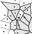
Figure 1.
Nucleus Cluster

Voronoï tessellation has great utility and has many applications such as the creation of synthetic poly-crystals, computer graphics [10], geodesy [11], non-parametric sampling [29] and geometric modelling in physics, astrophysics, chemistry and biology [5]. The form of clustering introduced in this article has proved to be important in the analysis of brain tissue [26], cortical activity and brain symmetries [28, 6] and capillary loss in skeletal and cardiac muscle [2]. Voronoï nucleus clustering also has great utility in the study of digital images (see,e.g., [21, §1.13], [1], [30]). The focus of this paper is not on the applications of MNCs, recently proved to be of great utility [28, 26]. Instead, the focus is on maximal nucleus clusters (MNCs) in proximity spaces and MNCs that are strongly proximal Edelsbrunner-Harer nerves. A proximity space setting for MNCs makes it possible to investigate the strong closeness of subsets in MNCs as well as the spatial and descriptive closeness of MNCs themselves.

2. Preliminaries

This section introduces the axioms for traditional as well as strong proximity spaces. Strong proximities were introduced in [23], elaborated in [21] (see, also, [13]) and are a direct result of earlier work on proximities [3, 4, 17, 18, 19].

2.1. Spatial and Descriptive Lodato Proximity

This section briefly introduces spatial and descriptive forms of proximity that provide a basis for two corresponding forms of strong Lodato proximity introduced in [23] and axiomatized in [21].

Let $X$ be a nonempty set. A Lodato proximity [14, 15, 16] $\delta$ is a relation on the family of sets $2^{X}$, which satisfies the following axioms for all subsets $A,B,C$ of $X$:

(P0):

$\emptyset\not\delta A,\forall A\subset X$.

(P1):

$A\ \delta\ B\Leftrightarrow B\delta A$.

(P2):

$A\ \cap\ B\neq\emptyset\Rightarrow A\delta B$.

(P3):

$A\ \delta\ (B\cup C)\Leftrightarrow A\ \delta\ B$ or $A\ \delta\ C$.

(P4):

$A\ \delta\ B$ and $\{b\}\ \delta\ C$ for each $b\in B\ \Rightarrow A\ \delta\ C$.   $\blacksquare$

Further $\delta$ is separated , if

(P5):

$\{x\}\ \delta\ \{y\}\Rightarrow x=y$.   $\blacksquare$

We can associate a topology with the space $(X,\delta)$ by considering as closed sets those sets that coincide with their own closure. For a nonempty set $A\subset X$, the closure of $A$ (denoted by $\mbox{cl}A$) is defined by,

$$\mbox{cl}A=\{x\in X:x\ \delta\ A\}.$$

The descriptive proximity $\delta_{\Phi}$ was introduced in [25]. Let $A,B\subset X$ and let $\Phi(x)$ be a feature vector for $x\in X$, a nonempty set of non-abstract points such as picture points. $A\ \delta_{\Phi}\ B$ reads $A$ is descriptively near $B$, provided $\Phi(x)=\Phi(y)$ for at least one pair of points, $x\in A,y\in B$. From this, we obtain the description of a set and the descriptive intersection [19, §4.3, p. 84] of $A$ and $B$ (denoted by $A\ \mathop{\cap}\limits_{\Phi}\ B$) defined by

($\boldsymbol{\Phi}$):

$\Phi(A)=\left\{\Phi(x)\in\mathbb{R}^{n}:x\in A\right\}$, set of feature vectors.

($\boldsymbol{\mathop{\cap}\limits_{\Phi}}$):

$A\ \mathop{\cap}\limits_{\Phi}\ B=\left\{x\in A\cup B:\Phi(x)\in\Phi(A)\ \mbox{and}\ \Phi(x)\in\Phi(B)\right\}$.   $\blacksquare$

Then swapping out $\delta$ with $\delta_{\Phi}$ in each of the Lodato axioms defines a descriptive Lodato proximity.

That is, a descriptive Lodato proximity $\delta_{\Phi}$ is a relation on the family of sets $2^{X}$, which satisfies the following axioms for all subsets $A,B,C$ of $X$.

(dP0):

$\emptyset\ {\not\delta}_{\Phi}\ A,\forall A\subset X$.

(dP1):

$A\ \delta_{\Phi}\ B\Leftrightarrow B\ \delta_{\Phi}\ A$.

(dP2):

$A\ \mathop{\cap}\limits_{\Phi}\ B\neq\emptyset\Rightarrow\ A\ \delta_{\Phi}\ B$.

(dP3):

$A\ \delta_{\Phi}\ (B\cup C)\Leftrightarrow A\ \delta_{\Phi}\ B$ or $A\ \delta_{\Phi}\ C$.

(dP4):

$A\ \delta_{\Phi}\ B$ and $\{b\}\ \delta_{\Phi}\ C$ for each $b\in B\ \Rightarrow A\ \delta_{\Phi}\ C$.   $\blacksquare$

Further $\delta_{\Phi}$ is descriptively separated , if

(dP5):

$\{x\}\ \delta_{\Phi}\ \{y\}\Rightarrow\Phi(x)=\Phi(y)$ ($x$ and $y$ have matching descriptions).   $\blacksquare$

The pair $\left(X,\delta_{\Phi}\right)$ is called a descriptive proximity space. Unlike the Lodato Axiom (P2), the converse of the descriptive Lodato Axiom (dP2) also holds.

Proposition 1.

Let $\left(X,\delta_{\Phi}\right)$ be a descriptive proximity space, $A,B\subset X$. Then $A\ \delta_{\Phi}\ B\Rightarrow A\ \mathop{\cap}\limits_{\Phi}\ B\neq\emptyset$.

Proof.

$A\ \delta_{\Phi}\ B\Leftrightarrow$ there is at least one $x\in A,y\in B$ such that $\Phi(x)=\Phi(y)$ (by definition of $A\ \delta_{\Phi}\ B$)  Hence, $A\ \mathop{\cap}\limits_{\Phi}\ B\neq\emptyset$. ∎

2.2. Spatial and Descriptive Strong Proximities

This section briefly introduces spatial strong proximity between nonempty sets and descriptive strong Lodato proximity.

Nonempty sets $A,B$ in a topological space $X$ equipped with the relation $\mathop{\delta}\limits^{\doublewedge}$, are strongly near [strongly contacted] (denoted $A\ \mathop{\delta}\limits^{\doublewedge}\ B$), provided the sets have at least one point in common. The strong contact relation $\mathop{\delta}\limits^{\doublewedge}$ was introduced in [20] and axiomatized in [24], [12, §6 Appendix].

Let $X$ be a topological space, $A,B,C\subset X$ and $x\in X$. The relation $\mathop{\delta}\limits^{\doublewedge}$ on the family of subsets $2^{X}$ is a strong proximity, provided it satisfies the following axioms.

(snN0):

$\emptyset\ \stackrel{{\scriptstyle\not{\text{\normalsize$\delta$}}}}{{\text{\tiny$\doublevee$}}}\ A,\forall A\subset X$, and  $X\ \mathop{\delta}\limits^{\doublewedge}\ A,\forall A\subset X$.

(snN1):

$A\mathop{\delta}\limits^{\doublewedge}B\Leftrightarrow B\mathop{\delta}\limits^{\doublewedge}A$.

(snN2):

$A\ \mathop{\delta}\limits^{\doublewedge}\ B$ implies $A\ \cap\ B\neq\emptyset$.

(snN3):

If $\{B_{i}\}_{i\in I}$ is an arbitrary family of subsets of $X$ and $A\mathop{\delta}\limits^{\doublewedge}B_{i^{*}}$ for some $i^{*}\in I\$ such that $\mbox{int}(B_{i^{*}})\neq\emptyset$, then $\ A\mathop{\delta}\limits^{\doublewedge}(\bigcup_{i\in I}B_{i})$

(snN4):

$\mbox{int}A\ \cap\ \mbox{int}B\neq\emptyset\Rightarrow A\ \mathop{\delta}\limits^{\doublewedge}\ B$.   $\blacksquare$

When we write $A\ \mathop{\delta}\limits^{\doublewedge}\ B$, we read $A$ is strongly near $B$ ($A$ strongly contacts $B$). The notation $A\ \mathop{\not{\delta}}\limits^{\doublewedge}\ B$ reads $A$ is not strongly near $B$ ($A$ does not strongly contact $B$). For each strong proximity (strong contact), we assume the following relations:

(snN5):

$x\in\mbox{int}(A)\Rightarrow x\ \mathop{\delta}\limits^{\doublewedge}\ A$

(snN6):

$\{x\}\ \mathop{\delta}\limits^{\doublewedge}\{y\}\ \Leftrightarrow x=y$   $\blacksquare$

For strong proximity of the nonempty intersection of interiors, we have that $A\mathop{\delta}\limits^{\doublewedge}B\Leftrightarrow\mbox{int}A\cap\mbox{int}B\neq\emptyset$ or either $A$ or $B$ is equal to $X$, provided $A$ and $B$ are not singletons; if $A=\{x\}$, then $x\in\mbox{int}(B)$, and if $B$ too is a singleton, then $x=y$. It turns out that if $A\subset X$ is an open set, then each point that belongs to $A$ is strongly near $A$. The bottom line is that strongly near sets always share points, which is another way of saying that sets with strong contact have nonempty intersection. Let $\delta$ denote a traditional proximity relation [17].

Figure 2. Near Sets: $A=\left\{(x,0):0.1\leq x\leq 1\right\},B=\left\{(x,sin(5/x)):0.1\leq x\leq 1\right\}$

Next, consider a proximal form of a Száz relator [27]. A proximal relator $\mathscr{R}$ is a set of relations on a nonempty set $X$ [22]. The pair $\left(X,\mathscr{R}\right)$ is a proximal relator space. The connection between $\mathop{\delta}\limits^{\doublewedge}$ and $\delta$ is summarized in Prop. 2.

Proposition 2.

Let $\left(X,\left\{\delta,\delta_{\Phi},\mathop{\delta}\limits^{\doublewedge}\right\}\right)$ be a proximal relator space, $A,B\subset X$. Then

1. $A\ \mathop{\delta}\limits^{\doublewedge}\ B\Rightarrow A\ \delta\ B$.

2. $A\ \mathop{\delta}\limits^{\doublewedge}\ B\Rightarrow A\ \delta_{\Phi}\ B$.

Proof.

1^o: From Axiom (snN2), $A\ \mathop{\delta}\limits^{\doublewedge}\ B$ implies $A\ \cap\ B\neq\emptyset$, which implies $A\ \delta\ B$ (from Lodato Axiom (P2)).
2^o: From 1^o, there are $x\in A,y\in B$ common to $A$ and $B$. Hence, $\Phi(x)=\Phi(y)$, which implies $A\ \mathop{\cap}\limits_{\Phi}\ B\neq\emptyset$. Then, from the descriptive Lodato Axiom (dP2), $A\ \mathop{\cap}\limits_{\Phi}\ B\neq\emptyset\Rightarrow\ A\ \delta_{\Phi}\ B$. This gives the desired result. ∎

Example 1.

Let $X$ be a topological space endowed with the strong proximity $\mathop{\delta}\limits^{\doublewedge}$ and $A=\left\{(x,0):0.1\leq x\leq 1\right\}$,$B=\left\{(x,sin(5/x)):0.1\leq x\leq 1\right\}$. In this case, $A,B$ represented by Fig. 2 are strongly near sets with many points in common.   $\blacksquare$

The descriptive strong proximity $\mathop{\delta_{{}_{\Phi}}}\limits^{\doublewedge}$ is the descriptive counterpart of $\mathop{\delta}\limits^{\doublewedge}$. To obtain a descriptive strong Lodato proximity (denoted by dsn), we swap out $\delta_{\Phi}$ in each of the descriptive Lodato axioms with the descriptive strong proximity $\mathop{\delta_{{}_{\Phi}}}\limits^{\doublewedge}$.

Let $X$ be a topological space, $A,B,C\subset X$ and $x\in X$. The relation $\mathop{\delta_{{}_{\Phi}}}\limits^{\doublewedge}$ on the family of subsets $2^{X}$ is a descriptive strong Lodato proximity, provided it satisfies the following axioms.

(dsnP0):

$\emptyset\ {\stackrel{{\scriptstyle\not{\text{\normalsize$\delta$}}}}{{\text{\tiny$\doublevee$}}}_{{}_{\Phi}}}\ A,\forall A\subset X$, and  $X\ \mathop{\delta_{{}_{\Phi}}}\limits^{\doublewedge}\ A,\forall A\subset X$.

(dsnP1):

$A\ \mathop{\delta_{{}_{\Phi}}}\limits^{\doublewedge}\ B\Leftrightarrow B\ \mathop{\delta_{{}_{\Phi}}}\limits^{\doublewedge}\ A$.

(dsnP2):

$A\ \mathop{\delta_{{}_{\Phi}}}\limits^{\doublewedge}\ B$ implies $A\ \mathop{\cap}\limits_{\Phi}\ B\neq\emptyset$.

(dsnP4):

$\mbox{int}A\ \mathop{\cap}\limits_{\Phi}\ \mbox{int}B\neq\emptyset\Rightarrow A\ \mathop{\delta_{{}_{\Phi}}}\limits^{\doublewedge}\ B$.   $\blacksquare$

When we write $A\ \mathop{\delta_{{}_{\Phi}}}\limits^{\doublewedge}\ B$, we read $A$ is descriptively strongly near $B$. For each descriptive strong proximity, we assume the following relations:

(dsnP5):

$\Phi(x)\in\Phi(\mbox{int}(A))\Rightarrow x\ \mathop{\delta_{{}_{\Phi}}}\limits^{\doublewedge}\ A$.

(dsnP6):

$\{x\}\ \mathop{\delta_{{}_{\Phi}}}\limits^{\doublewedge}\ \{y\}\Leftrightarrow\Phi(x)=\Phi(y)$.   $\blacksquare$

So, for example, if we take the strong proximity related to non-empty intersection of interiors, we have that $A\ \mathop{\delta_{{}_{\Phi}}}\limits^{\doublewedge}\ B\Leftrightarrow\mbox{int}A\ \mathop{\cap}\limits_{\Phi}\ \mbox{int}B\neq\emptyset$ or either $A$ or $B$ is equal to $X$, provided $A$ and $B$ are not singletons; if $A=\{x\}$, then $\Phi(x)\in\Phi(\mbox{int}(B))$, and if $B$ is also a singleton, then $\Phi(x)=\Phi(y)$.

The connections between $\mathop{\delta_{{}_{\Phi}}}\limits^{\doublewedge},\delta_{\Phi}$ are summarized in Prop. 3.

Proposition 3.

Let $\left(X,\left\{\mathop{\delta}\limits^{\doublewedge},\delta_{\Phi},\mathop{\delta_{{}_{\Phi}}}\limits^{\doublewedge}\right\}\right)$ be a proximal relator space, $A,B\subset X$. Then

1. For $A,B$ not equal to singletons, $A\ \mathop{\delta_{{}_{\Phi}}}\limits^{\doublewedge}\ B\Rightarrow\mbox{int}A\ \mathop{\cap}\limits_{\Phi}\ \mbox{int}B\neq\emptyset\Rightarrow\mbox{int}A\ \delta_{\Phi}\ \mbox{int}B$.

2. $A\ \mathop{\delta}\limits^{\doublewedge}\ B\Rightarrow(\mbox{int}A\ \mathop{\cap}\limits_{\Phi}\ \mbox{int}B)\ \mathop{\delta_{{}_{\Phi}}}\limits^{\doublewedge}\ B$.

3. $A\ \mathop{\delta_{{}_{\Phi}}}\limits^{\doublewedge}\ B\Rightarrow A\ \delta_{\Phi}\ B$.

Proof.

1^o: $A\ \mathop{\delta_{{}_{\Phi}}}\limits^{\doublewedge}\ B$ implies that interior of $A$ is descriptively near the interior of $B$. Consequently, $\mbox{int}A\ \mathop{\cap}\limits_{\Phi}\ \mbox{int}B\neq\emptyset$. Hence, from Axiom (dP2), $\mbox{int}A\ \delta_{\Phi}\ \mbox{int}B$.
1${}^{o}\Rightarrow\ 2^{o}$. 3^o: Immediate from Axioms (dsnP2) and (dP2). ∎

2.3. Voronoï regions

Let $E$ be the Euclidean plane, $S\subset E$ (set of mesh generating points), $s\in S$. A Voronoï region (denoted by $V(s)$) is defined by

$$V(s)=\left\{x\in E:\left\|x-s\right\|\leq\left\|x-q\right\|,\mbox{for all}\ q\in S\right\}\ \mbox{(Vorono\"{i} region)}.$$

Let $X$ be a collection of Voronoï regions containing $N$, endowed with the strong proximity $\mathop{\delta}\limits^{\doublewedge}$. A nucleus mesh cluster (denoted by $\mbox{\large$\mathfrak{C}$}\ N$) in a Voronoï tessellation is defined by

$$\mbox{\large$\mathfrak{C}$}\ N=\left\{A\in X:\mbox{cl}\ A\ \mathop{\delta}\limits^{\doublewedge}\ N\right\}\ \mbox{(Vorono\"{i} mesh nucleus cluster)}.\\$$

Example 2.

A partial view of a Voronoï tessellation of a plane surface is shown in Fig. 1. The Voronoï region $N$ in this tessellation is the nucleus of a mesh cluster containing all of those polygons adjacent to $N$.   ◼

A concrete (physical) set $A$ of points $p$ that are described by their location and physical characteristics, e.g., gradient orientation (angle of the tangent to $p$. Let $\varphi(p)$ be the gradient orientation of $p$. For example, each point $p$ with coordinates $(x,y)$ in the concrete subset $A$ in the Euclidean plane is described by a feature vector of the form $(x,y,\varphi(p(x,y))$. Nonempty concrete sets $A$ and $B$ have descriptive strong proximity (denoted $A\ \mathop{\delta_{{}_{\Phi}}}\limits^{\doublewedge}\ B$), provided $A$ and $B$ have points with matching descriptions. In a region-based, descriptive proximity extends to both abstract and concrete sets [21, §1.2]. For example, every subset $A$ in the Euclidean plane has features such as area and diameter. Let $(x,y)$ be the coordinates of the centroid $m$ of $A$. Then $A$ is described by feature vector of the form $(x,y,area,diameter)$. Then regions $A,B$ have descriptive proximity (denoted $A\ \mathop{\delta_{{}_{\Phi}}}\limits^{\doublewedge}\ B$), provided $A$ and $B$ have matching descriptions.

The notion of strongly proximal regions extends to convex sets. A nonempty set $A$ is a convex set (denoted $\mbox{conv}A$), provided, for any pair of points $x,y\in A$, the line segment $\overline{xy}$ is also in $A$. The empty set $\emptyset$ and a one-element set $\left\{x\right\}$ are convex by definition. Let $\mathscr{F}$ be a family of convex sets. From the fact that the intersection of any two convex sets is convex [7, §2.1, Lemma A], it follows that

$$\mathop{\bigcap}\limits_{A\in\mathscr{F}}A\ \mbox{is a convex set}.$$

Convex sets $\mbox{conv}A,\mbox{conv}B$ are strongly proximal (denote $\mbox{conv}A\mathop{\delta}\limits^{\doublewedge}\ \mbox{conv}B$), provided $\mbox{conv}A,\mbox{conv}B$ have points in common. Convex sets $\mbox{conv}A,\mbox{conv}B$ are descriptively strongly proximal (denoted $\mbox{conv}A\mathop{\delta_{{}_{\Phi}}}\limits^{\doublewedge}\ \mbox{conv}B$), provided $\mbox{conv}A,\mbox{conv}B$ have matching descriptions.

Let $X$ be a Voronoï tessellation of a plane surface equipped with the strong proximity $\mathop{\delta}\limits^{\doublewedge}$ and descriptive strong proximity $\mathop{\delta_{{}_{\Phi}}}\limits^{\doublewedge}$ and let $A,N\in X$ be Voronoï regions. The pair $\left(X,\left\{\mathop{\delta}\limits^{\doublewedge},\mathop{\delta_{{}_{\Phi}}}\limits^{\doublewedge}\right\}\right)$ is an example of a proximal relator space [22]. The two forms of nucleus clusters (ordinary nucleus cluster denoted by $\mathfrak{C}$) and descriptive nucleus clusters are examples of mesh nerves [21, §1.10, pp. 29ff], defined by

$$\mbox{\large$\mathfrak{C}$}N =\left\{A\in X:A\ \mathop{\delta}\limits^{\doublewedge}\ N\right\}\ \mbox{(nucleus cluster)}.$$

$$\mathfrak{C}_{\Phi}N =\left\{A\in X:A\ \mathop{\delta_{{}_{\Phi}}}\limits^{\doublewedge}\ N\right\}\ \mbox{(descriptive nucleus cluster)}.$$

A nucleus cluster is maximal (denoted by $\mbox{max}\mathfrak{C}N$), provided $N$ has the highest number of adjacent polygons in a tessellated surface (more than one maximal cluster in the same mesh is possible). Similarly, a descriptive nucleus cluster is maximal (denoted by $\mbox{max}\mathfrak{C}_{\Phi}N$), provided $N$ has the highest number of polygons in a tessellated surface descriptively near $N$, i.e., the description of each $A\in\mbox{max}\mathfrak{C}_{\Phi}N$ matches the description of nucleus $N$ and the number of polygons descriptively near $N$ is maximal (again, more than one $\mbox{max}\mathfrak{C}_{\Phi}N$ is possible in a Voronoï tessellation).

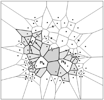
Figure 3. $\mbox{\large$\mathfrak{C}$}\ N_{1}\ \mathop{\delta}\limits^{\doublewedge}\ \mbox{\large$\mathfrak{C}$}\ N_{2}\ \mbox{and}\ \mbox{\large$\mathfrak{C}$}\ N_{1}\ \mathop{\delta_{{}_{\Phi}}}\limits^{\doublewedge}\ \mbox{\large$\mathfrak{C}$}\ N_{2}$

Example 3.

Let $X$ be the collection of Voronoï regions in a tessellation of a subset of the Euclidean plane shown in Fig. 3 with nuclei $N_{1},N_{2},N_{3}\in X$. In addition, let $2^{X}$ be the family of all subsets of Voronoï regions in $X$ containing maximal nucleus clusters $\mbox{\large$\mathfrak{C}$}N_{1},\mbox{\large$\mathfrak{C}$}N_{2},\mbox{\large$\mathfrak{C}$}N_{3}\in 2^{X}$ in the tessellation. Then, for example, $\mbox{int}\mbox{\large$\mathfrak{C}$}N_{2}\ \cap\ \mbox{int}\mbox{\large$\mathfrak{C}$}N_{3}\neq\emptyset$, since $\mbox{\large$\mathfrak{C}$}N_{2},\mbox{\large$\mathfrak{C}$}N_{3}$ share Voronoï regions. Hence, $\mbox{\large$\mathfrak{C}$}N_{2}\ \mathop{\delta}\limits^{\doublewedge}\ \mbox{\large$\mathfrak{C}$}N_{3}\neq\emptyset$ (from Axiom (snN4)). Similarly, $\mbox{\large$\mathfrak{C}$}N_{1}\ \mathop{\delta}\limits^{\doublewedge}\ \mbox{\large$\mathfrak{C}$}N_{2}$.

Let $\Phi(A)$ the description of a Voronoï equal the number of sides of $A\in X$. Since the nuclei $N_{1},N_{2},N_{3}$ have matching descriptions, $\mbox{int}\mbox{\large$\mathfrak{C}$}N_{1}\ \mathop{\cap}\limits_{\Phi}\ \mbox{int}\mbox{\large$\mathfrak{C}$}N_{2}\neq\emptyset$. Consequently, $\mbox{\large$\mathfrak{C}$}N_{1}\ \mathop{\delta_{{}_{\Phi}}}\limits^{\doublewedge}\ \mbox{\large$\mathfrak{C}$}N_{2}$ (from Axiom (dsnP4)). Similarly, $\mbox{\large$\mathfrak{C}$}N_{1}\ \mathop{\delta_{{}_{\Phi}}}\limits^{\doublewedge}\ \mbox{\large$\mathfrak{C}$}N_{3}$ and $\mbox{\large$\mathfrak{C}$}N_{2}\ \mathop{\delta_{{}_{\Phi}}}\limits^{\doublewedge}\ \mbox{\large$\mathfrak{C}$}N_{3}$.   ◼

Figure 4.
MNC Spokes

3. Main Results

Homotopy types are introduced in [9, §III.2] and lead to significant results for Voronoï maximal nucleus clusters.

Let $f,g:X\longrightarrow Y$ be two continuous maps. A homotopy between $f$ and $g$ is a continuous map $H:X\times[0,1]\longrightarrow Y$ so that $H(x,0)=f(x)$ and $H(x,1)=g(x)$. The sets $X$ and $Y$ are homotopy equivalent, provided there are continuous maps $f:X\longrightarrow Y$ and $g:Y\longrightarrow X$ such that $g\circ f\simeq\mbox{id}_{X}$ and $f\circ g\simeq\mbox{id}_{Y}$. This yields an equivalence relation $X\simeq Y$. In addition, $X$ and $Y$ have the same homotopy type, provided $X$ and $Y$ are homotopy equivalent.

Let $\mathscr{F}$ be a finite collection of sets. An Edelsbrunner-Harer nerve (denoted by $\mbox{Nrv}\ \mathscr{F}$) consists of all nonempty subcollections of $\mathscr{F}$ that have a nonvoid common intersection, i.e.,

$$\mbox{Nrv}\ \mathscr{F}=\left\{X\in\mathscr{F}:\bigcap X\neq\emptyset\right\}.$$

Let $\mathscr{F}_{{}_{MNC}}$ be a collection of polygons in a Voronoï MNC endowed with the strong proximity $\mathop{\delta}\limits^{\doublewedge}$, $A$ be a Voronoï region in a MNC $\mbox{\large$\mathfrak{C}$}N$ with nucleus $N$ and let subscollection $\mathscr{S}_{A}=\left\{A,N\right\}\in\mbox{\large$\mathfrak{C}$}N$. The pair $\left(\mathscr{F}_{{}_{MNC}},\mathop{\delta}\limits^{\doublewedge}\right)$ is a proximity space. For each MNC $\mbox{\large$\mathfrak{C}$}N$ endowed with $\mathop{\delta}\limits^{\doublewedge}$, the nucleus $N$ together with its adjacent polygons is a Voronoï structure (denoted by $\mbox{Nrv}\mathscr{F}_{{}_{MNC}}$) defined by

$$\mbox{Nrv}\mathscr{F}_{{}_{MNC}}=\left\{\mathscr{S}\in\mbox{\large$\mathfrak{C}$}N:\left(N,A\right)\in\mathop{\delta}\limits^{\doublewedge}\ \mbox{for}\ A\in\mathscr{S}\right\}\ \mbox{(MNC nerve)}.$$

Each pair $\left(N,A\right)\in\mathop{\delta}\limits^{\doublewedge}$ in $\mbox{Nrv}\mathscr{F}_{{}_{MNC}}$ is called a spoke (denoted by $\mathscr{S}_{A}$), with a shape similar to the spoke in a wheel. A spoke contains a Voronoï region $A\in\mbox{\large$\mathfrak{C}$}N$ that shares an edge with $N$. Hence, the $A\ \mathop{\delta}\limits^{\doublewedge}\ N$, i.e., there is a strong proximity between the subsets in a spoke.

Example 4.

A pair of spokes $\mathscr{S}_{A_{1}},\mathscr{S}_{A_{2}}$ in a fragment of an MNC $\mbox{\large$\mathfrak{C}$}N$ with nucleus $N$ is represented in Fig. 4.   ◼

Every MNC $\mbox{\large$\mathfrak{C}$}N$ is a finite collection of closed convex sets in the Euclidean plane. Let $\mbox{\large$\mathfrak{C}$}N$ be endowed with the strong proximity $\mathop{\delta}\limits^{\doublewedge}$. All non-nucleus polygons in $\mbox{\large$\mathfrak{C}$}N$ share an edge with $N$. The collection of spokes $\mathscr{S}_{A}\in\mbox{\large$\mathfrak{C}$}N$ each contain the nucleus $N$, which is common to all of the spokes, i.e., the spokes in $\mbox{Nrv}\mathscr{F}_{{}_{MNC}}$ have a nonvoid common intersection. Let $\mathscr{S}_{A},\mathscr{S}_{A^{\prime}}$ be spokes in $\mbox{\large$\mathfrak{C}$}N$ that share nucleus $N$. Consequently, $\mbox{int}\left(\mathscr{S}_{A}\right)\ \cap\ \mbox{int}\left(\mathscr{S}_{A^{\prime}}\right)\neq\emptyset$ implies $\mathscr{S}_{A}\ \mathop{\delta}\limits^{\doublewedge}\ \mathscr{S}_{A^{\prime}}$ (from Axiom (snN4)). Hence, $\mbox{Nrv}\mathscr{F}_{{}_{MNC}}$ is an Edelsbrunner-Harer nerve. From this, we obtain the result in Lemma 1.

Lemma 1.

Let $\mathscr{F}_{{}_{MNC}}$ be a collection of polygons in a Voronoï MNC endowed with the strong proximity $\mathop{\delta}\limits^{\doublewedge}$. The structure $\mbox{Nrv}\mathscr{F}_{mnc}$ is an Edelsbrunner-Harer nerve.

Proof.

Let $\mathscr{S}_{A},\mathscr{S}_{A^{\prime}}$ be a pair of spokes in a maximal nucleus cluster MNC $\mbox{\large$\mathfrak{C}$}N$. Since $\mathscr{S}_{A}\ \mathop{\delta}\limits^{\doublewedge}\ \mathscr{S}_{A^{\prime}}$ have $N$ in common, $\mathscr{S}_{A}\mathop{\delta}\limits^{\doublewedge}\mathscr{S}_{A^{\prime}}$ implies $\mathscr{S}_{A}\cap\mathscr{S}_{A^{\prime}}\neq\emptyset$ (from Axiom (snN2)). This holds true for all spokes in $\mbox{\large$\mathfrak{C}$}N$. Consequently, $\mathop{\bigcap}\limits_{\mathscr{S}_{A}\in\mbox{\large$\mathfrak{C}$}N}\mathscr{S}_{A}\neq\emptyset$. Hence, the structure $\mbox{Nrv}\mathscr{F}_{{}_{MNC}}$ is an Edelsbrunner-Harer nerve. ∎

Theorem 1.

Let $\left(\mbox{Nrv}\mathscr{F}_{{}_{MNC}},\left\{\delta,\delta_{\Phi},\mathop{\delta}\limits^{\doublewedge}\right\}\right)$ be a proximal relator space, spokes $\mathscr{S}_{A},\mathscr{S}_{A^{\prime}}\in\mbox{Nrv}\mathscr{F}_{{}_{MNC}}$. Then

1. $\mathscr{S}_{A}\ \mathop{\delta}\limits^{\doublewedge}\ \mathscr{S}_{A^{\prime}}\Rightarrow\mathscr{S}_{A}\ \delta\ \mathscr{S}_{A^{\prime}}$.

2. $\mathscr{S}_{A}\ \mathop{\delta}\limits^{\doublewedge}\ \mathscr{S}_{A^{\prime}}\Rightarrow\mathscr{S}_{A}\ \delta_{\Phi}\ \mathscr{S}_{A^{\prime}}$.

Proof.

1^o: From Lemma 1, $\mbox{Nrv}\mathscr{F}_{{}_{MNC}}$ is an Edelsbrunner-Harer nerve. Consequently, $\mathscr{S}_{A}\ \mathop{\delta}\limits^{\doublewedge}\ \mathscr{S}_{A^{\prime}}$ for every pair of spokes $\mathscr{S}_{A},\mathscr{S}_{A^{\prime}}$ in the nerve. Then, $\mathscr{S}_{A}\ \mathop{\delta}\limits^{\doublewedge}\ \mathscr{S}_{A^{\prime}}$ implies $\mathscr{S}_{A}\ \cap\ \mathscr{S}_{A^{\prime}}\neq\emptyset$, which implies $\mathscr{S}_{A}\ \delta\ \mathscr{S}_{A^{\prime}}$ (from Prop. 2).
2^o: Spokes $\mathscr{S}_{A},\mathscr{S}_{A^{\prime}}$ have nucleus $N$ in common. Hence, $\mathscr{S}_{A}\ \mathop{\cap}\limits_{\Phi}\ \mathscr{S}_{A^{\prime}}\neq\emptyset$. Then, from Prop. 2, $\mathscr{S}_{A}\ \mathop{\cap}\limits_{\Phi}\ \mathscr{S}_{A^{\prime}}\neq\emptyset\Rightarrow\ \mathscr{S}_{A}\ \delta_{\Phi}\ \mathscr{S}_{A^{\prime}}$. This gives the desired result for each pair of spokes in the nerve. ∎

Theorem 2.

[9, §III.2, p. 59] Let $\mathscr{F}$ be a finite collection of closed, convex sets in Euclidean space. Then the nerve of $\mathscr{F}$ and the union of the sets in $\mathscr{F}$ have the same homotopy type.

Theorem 3.

Let the nucleus cluster $\mbox{\large$\mathfrak{C}$}N$ be a finite collection of closed, convex sets in a Voronoï mesh $V$ in the Euclidean plane. The nerve $\mbox{Nrv}\mathscr{F}_{MNC}$ in $\mbox{\large$\mathfrak{C}$}N$ and the union of the sets in $\mbox{\large$\mathfrak{C}$}N$ have the same homotopy type.

Proof.

Let $\mbox{\large$\mathfrak{C}$}N$ be a MNC be nucleus $N$ in a Voronoï mesh. From Lemma 1, $\mbox{Nrv}\mathscr{F}_{{}_{MNC}}$ is a Edelsbrunner-Harer nerve. From Theorem 2, we have that the union of the sets in $\mbox{\large$\mathfrak{C}$}N$ and $\mbox{Nrv}\mathscr{F}_{{}_{MNC}}$ have the same homotopy type. ∎

Theorem 4.

Let $X$ be a finite collection of MNC Edelsbrunner-Harer nerves $\mbox{Nrv}\mathscr{F}_{{}_{MNC}}$ in a Voronoï mesh with nuclei $N$ in the Euclidean plane and let $X$ be equipped with the relator $\left\{\mathop{\delta}\limits^{\doublewedge},\mathop{\delta_{{}_{\Phi}}}\limits^{\doublewedge}\right\}$ with strongly close mesh nerves. Each nucleus $N$ has a description $\Phi(N)=\mbox{number of sides of}\ N$. Then $\mathop{\bigcap}\limits_{\Phi}\mbox{Nrv}\mathscr{F}_{{}_{MNC}}\neq\emptyset$.

Proof.

Each $\mbox{Nrv}\mathscr{F}_{{}_{MNC}}$ is a collection of Voronoï regions containing a nucleus polygon $N$ with the same number of sides, since $\mbox{Nrv}\mathscr{F}_{{}_{MNC}}\in\mbox{\large$\mathfrak{C}$}N$, which is maximal. Let $\mathscr{N},\mathscr{N^{\prime}}\in X$ be nerves with nuclei $N_{1},N_{2}$ in maximal nucleus clusters. $\Phi(N_{1})=\Phi(N_{2})$, since $\mbox{\large$\mathfrak{C}$}N_{1},\mbox{\large$\mathfrak{C}$}N_{2}$ are maximal, i.e., $N_{1},N_{2}$ have same number of sides. This means that all nuclei in $\mathscr{N},\mathscr{N^{\prime}}$ have the same description. Consequently, $\mathscr{N}\ \mathop{\delta_{{}_{\Phi}}}\limits^{\doublewedge}\ \mathscr{N^{\prime}}$ implies $\mbox{int}N_{1}\ \mathop{\cap}\limits_{\Phi}\ \mbox{int}N_{2}\neq\emptyset$ (from Axiom (dsnP2)). Hence, $N_{1}\ \mathop{\delta_{{}_{\Phi}}}\limits^{\doublewedge}\ N_{2}$ implies $\mathscr{N}\ \delta_{\Phi}\ \mathscr{N^{\prime}}$ (from Prop. 3). Then $\mathscr{N}\ \delta_{\Phi}\ \mathscr{N^{\prime}}$ implies $\mathscr{N}\ \mathop{\cap}\limits_{\Phi}\ \mathscr{N^{\prime}}\neq\emptyset$ (from Prop. 1). Therefore, $\mathop{\bigcap}\limits_{\Phi}\mbox{Nrv}\mathscr{F}_{{}_{MNC}}\neq\emptyset$. ∎

References

• [1] E. A-iyeh and J.F. Peters, Measure of tessellation quality of voronoï meshes, Theory and Application of Math. and Comp. Sci. 5 (2015), no. 2, 158–185.
• [2] A. Al-Shammari, E.A. Gaffney, and S. Egginton, Re-evaluating the use of voronoi tessellations in the assessment of oxygen supply from capillaries in muscle, Bull. Math. Biol. 74 (2016), no. 9, 2204 –2231, MR2964894.
• [3] A. Di Concilio, Topologizing homeomorphism groups of rim-compact spaces, Topology and its Applications 153 (2006), no. 11, 1867–1885.
• [4] by same author, Point-free geometries: Proximities and quasi-metrics, Math. in Comp. Sci. 7 (2013), no. 1, 31–42, MR3043916.
• [5] Q. Du and M. Gunzburger, Advances in studies and applications of centroidal voronoi tessellations, Numer. Math. Theory Methods Appl. 3 (2010), no. 2, 119 –142, MR2682789.
• [6] G. Duyckaerts and G. Godefroy, Voronoï tessellation to study the numerical density and the spatial distribution of neurons, J. of Chemical Neuroanatomy 20 (2000), no. 1, 83–92.
• [7] H. Edelsbrunner, A short course in computational geometry and topology, Springer, Berlin, 2014, 110 pp.
• [8] H. Edelsbrunner and J.L. Harer, Computational topology. an introduction, American Mathematical Society, Providence, R.I., 2010, xii+110 pp., MR2572029.
• [9] by same author, Computational topology. an introduction, Amer. Math. Soc., Providence, RI, 2010, xii+241 pp. ISBN: 978-0-8218-4925-5, MR2572029.
• [10] S. Fukushige and H. Suzuki, Polygon visibility ordering via voronoi diagrams, Visual Comput. 23 (2007), no. 7, 503 –511.
• [11] C. Gold, A common spatial model for gis, Research Trends in Geographic Information Science (G. Navratil, ed.), Springer, 2009, pp. 79–94.
• [12] C. Guadagni, Bornological convergences on local proximity spaces and $\omega_{\mu}$-metric spaces, Ph.D. thesis, Università degli Studi di Salerno, Salerno, Italy, 2015, Supervisor: A. Di Concilio, 79pp.
• [13] E. İnan, Algebraic structures on nearness approximation spaces, Ph.D. thesis, Department of Mathematics, 2015, supervisors: S. Keleş and M.A. Öztürk, vii+113pp.
• [14] M.W. Lodato, On topologically induced generalized proximity relations, ph.d. thesis, Rutgers University, 1962, supervisor: S. Leader.
• [15] by same author, On topologically induced generalized proximity relations i, Proc. Amer. Math. Soc. 15 (1964), 417–422.
• [16] by same author, On topologically induced generalized proximity relations ii, Pacific J. Math. 17 (1966), 131–135.
• [17] S.A. Naimpally, Proximity spaces, Cambridge University Press, Cambridge,UK, 1970, x+128 pp., ISBN 978-0-521-09183-1.
• [18] by same author, Proximity approach to problems in topology and analysis, Oldenbourg Verlag, Munich, Germany, 2009, 73 pp., ISBN 978-3-486-58917-7, MR2526304.
• [19] S.A. Naimpally and J.F. Peters, Topology with applications. topological spaces via near and far, World Scientific, Singapore, 2013, xv + 277 pp, Amer. Math. Soc. MR3075111.
• [20] J.F. Peters, Proximal Delaunay triangulation regions, Proceedings of the Jangjeon Math. Soc. 18 (2015), no. 4, 501–515, MR3444736.
• [21] by same author, Computational proximity. Excursions in the topology of digital images., Intelligent Systems Reference Library 102 (2016), xxvi + 433pp, DOI: 10.1007/978-3-319-30262-1, in press.
• [22] by same author, Proximal relator spaces, Filomat (2016), accepted.
• [23] J.F. Peters and C. Guadagni, Strong proximities on smooth manifolds and Voronoï diagrams, Advances in Math.: Sci. J. 4 (2015), no. 2, 91–107.
• [24] by same author, Strongly near proximity and hyperspace topology, arXiv 1502 (2015), no. 05913, 1–6.
• [25] J.F. Peters and S.A. Naimpally, Applications of near sets, Notices of the Amer. Math. Soc. 59 (2012), no. 4, 536–542, DOI: http://dx.doi.org/10.1090/noti817, MR2951956.
• [26] J.F. Peters, A. Tozzi, and S. Rananna, Brain tissue tessellation shows absence of canonical microcircuits, Neuroscience Letters (2016), in press.
• [27] Á Száz, Basic tools and mild continuities in relator spaces, Acta Math. Hungar. 50 (1987), no. 3-4, 177–201, MR0918156.
• [28] A. Tozzi and J.F. Peters, A topological approach unveils system invariances and broken symmetries in the brain, J. of Neuroscience Research (2016), 361–365, DOI: 10.1002/jnr.23720.
• [29] A. Villagran, G. Huerta, M. Vannucci, C.S. Jackson, and A. Nosedal, Non-parametric sampling approximation via voronoï tessellation, Comm. Statist. Simulation Comput. 45 (2016), no. 2, 717–736, MR3457116.
• [30] J. Wang, Edge-weighted centroidal voronoi tessellation based algorithms for image segmentation, Ph.D. thesis, Department of Scientific Computing, 2011, supervisors: X. Wang, xvi+96pp., MR2982159.