Non-adiabatic geometric phases and dephasing in an open quantum system Non-adiabatic geometric phases and dephasing in an open quantum system A.E. Svetogorov, Yu. Makhlin

Non-adiabatic geometric phases and dephasing in an open quantum system

Abstract

We analyze the influence of a dissipative environment on geometric phases in a quantum system subject to non-adiabatic evolution. We find dissipative contributions to the acquired phase and modification of dephasing, considering the cases of weak short-correlated noise as well as of slow quasi-stationary noise. Motivated by recent experiments, we find the leading non-adiabatic corrections to the results, known for the adiabatic limit.

The Berry phase [1] is a celebrated instance of geometric phases in physics [2], which occurs during adiabatic evolution of a quantum system. In the analysis of generalizations of the Berry phase, Aharonov and Anandan found a geometric phase even for non-adiabatic evolutions [3]. When a quantum system is coupled to an environment, phases, acquired by the system during its evolution, are modified. In particular, it was shown that in a quantum system subject simultaneously to adiabatic variation of its parameters and to weak short-correlated external noise, the phase acquires a geometric environment-induced contribution [4, 5]. Furthermore, the environment-induced decoherence is modulated by the parameter variation, which results in a geometric contribution to dephasing [4, 6]. Here we analyze the dynamics of an open quantum system during non-adiabatic evolution. In this case in a closed system the total phase is a combination of the dynamical phase and the geometric Aharonov-Anandan phase. We find, how this phase is modified by the environment. In particular, motivated by recent experiments with superconducting qubits, we study the adiabatic limit and find the leading non-adiabatic corrections.

The Berry phase was measured directly, in the original setting with cyclic variation of the magnetic field, in NMR systems [7]. Some time ago the degree of control over the quantum state and the coherence level allowed for direct observation of the Berry phase in superconducting qubits [8]. In later experiments, the influence of noise on the Berry phase in this system was studied and the geometric dephasing was analyzed [9, 10].

We first describe the coherent Aharonov-Anandan phase and then consider the influence of dissipation. We consider a quantum two-level system and use the spin-1/2 language for its description. The Hamiltonian of a two-state system can be presented as $H=-\bm{{\rm B}}(t)\bm{\sigma}/2$, where $\bm{{\rm B}}$ can be referred to as the (pseudo)magnetic field. For any variation of $\bm{{\rm B}}(t)$ over a certain period, $0<t<T$, the unitary evolution operator has two eigenstates, referred to as cyclic states as they return to their initial values up to a phase, i.e., the two corresponding opposite spin vectors return to their initial directions. The relative phase between these states acquired over the time $T$ defines the angle of rotation in spin space over the cyclic direction. Aharonov and Anandan [3] showed that it consists of two contributions defined below, a dynamical and geometric phase. Indeed, let $\bm{{\rm S}}(t)$ be a cyclic state. Consider a spin frame with the $z^{\prime}$ axis along $\bm{{\rm S}}(t)$. The magnetic field in this frame is $\bm{{\rm B}}^{\prime}=\bm{{\rm B}}+\bm{\omega}$, where $\bm{\omega}$ is the angular velocity of the rotating frame relative to the lab frame. Since the equation of motion in this frame reads $\dot{\bm{{\rm S}}}=\bm{{\rm S}}\times\bm{{\rm B}}^{\prime}$, and $\bm{{\rm S}}$ is stationary, $\bm{{\rm B}}^{\prime}$ has the same direction, $\bm{{\rm B}}^{\prime}\parallel\bm{{\rm S}}$. Thus the total relative phase between $\bm{{\rm S}}$ and $-\bm{{\rm S}}$, picked during the evolution, is given by $\int dtB^{\prime}=\int dtB_{\parallel}+\int dt\omega_{\parallel}$, where the subindex $\parallel$ indicates projection onto $\bm{{\rm S}}$. The first contribution to this total phase, also given by $\int dt\left\langle\psi\right|H\left|\psi\right\rangle$, the time integral of the average energy, is the dynamical phase (here $\left|\psi(t)\right\rangle$ is the quantum state, corresponding to $\bm{{\rm S}}(t)$). The rest, $\int dt\omega_{\parallel}$, similar to the case of the adiabatic evolution, is given by the solid angle, subtended by $\bm{{\rm S}}(t)$. This geometric contribution is the Aharonov-Anandan phase.

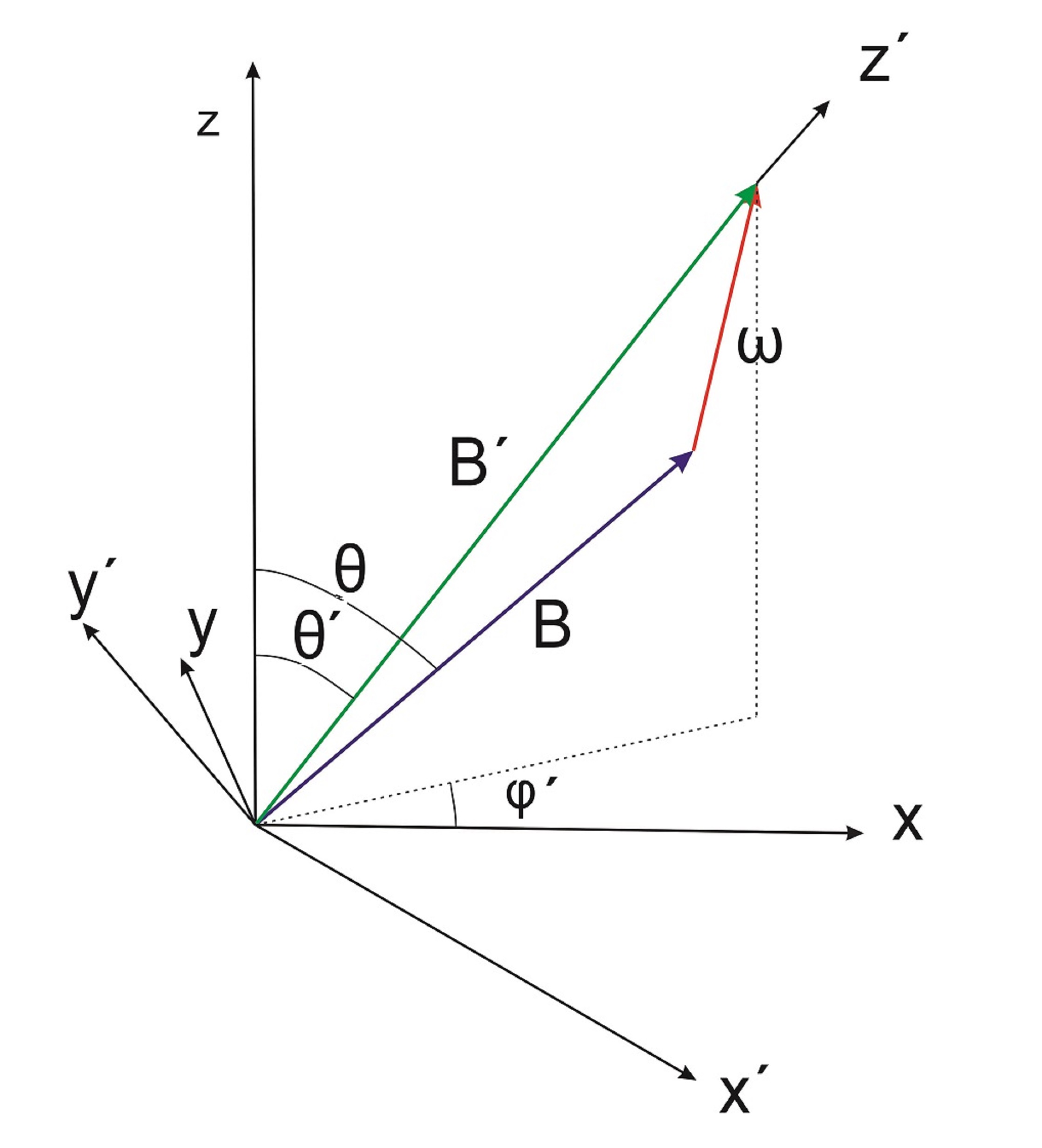
Figure 1: The rotating spin reference frame $x^{\prime}y^{\prime}z^{\prime}$, rotating with angular velocity $\bm{\omega}$ relative to the stationary frame $xyz$.

When the system is subject to external noise (coupled to an environment), its dynamics is modified. For a static field $\bm{{\rm B}}$, dissipation induces relaxation and dephasing, as well as a modification of the dynamical phase. For weak short-correlated noise, it was shown [4] that for an adiabatically slowly varying field, on top of that dissipation modifies the geometric Berry phase and introduces a geometric contribution to dephasing. Here we extend this analysis to the case of non-adiabatic evolution. We find the acquired phase and dephasing for a system coupled to environment and subject to non-adiabatic manipulations.

Consider a quantum system, a spin-1/2 in our case, coupled to an environment:

$$H=-\frac{1}{2}\bm{{\rm B}}\bm{\sigma}-\frac{1}{2}\bm{{\rm X}}\bm{\sigma}+H_{\rm env},$$ (1)

where $\bm{{\rm X}}=X\bm{{\rm n}}$ is an operator of the environment, which represents noise experienced by the quantum system (we assume $\langle X\rangle=0$); $H_{\rm env}$ governs the dynamics of the modes of the environment. To be specific, we consider unidirectional noise with $\bm{{\rm n}}=\hat{z}$. Such anisotropy of the noise is relevant, e.g., for superconducting qubits, where different (pseudo-)spin directions correspond to different physical variables [11]. We comment on other situations later.

In the rotating frame (RF), with the $z^{\prime}$-axis chosen along $\bf S$ and the $y^{\prime}$-axis orthogonal to the original $z$-axis (this choice ensures that the frame returns to its initial state after a cycle), the Hamiltonian reads

$$\hat{H}^{\prime}=-\frac{1}{2}B^{\prime}\sigma_{z^{\prime}}+\hat{H}_{int}+H_{env}$$ (2)

with the interaction term

$$\hat{H}_{int}=-\frac{1}{2}X\left(\cos\theta^{\prime}\sigma_{z^{\prime}}-\sin\theta^{\prime}\sigma_{x^{\prime}}\right)\,,$$

where $\theta^{\prime}$ is the angle between the direction $z$ of the fluctuations and the $z^{\prime}$ axis.

The phases can be read off from the off-diagonal element of the density matrix in the RF, $\langle\sigma_{x^{\prime}}+i\sigma_{y^{\prime}}\rangle=\rho_{\uparrow\downarrow}$. Using the real-time Keldysh technique [12, 11], we can derive the kinetic equation for the density matrix. For weak noise with a short correlation time $\tau_{c}\ll T_{1},T_{2}$ (here $T_{1},T_{2}$ are the longitudinal and transverse relaxation times) one can use the Bloch-Redfield and the rotating-wave approximations to find a closed equation for the off-diagonal entry $\rho_{\uparrow\downarrow}$:

$$\frac{d}{dt}\rho_{\uparrow\downarrow}(t)=iB^{\prime}\rho_{\uparrow\downarrow}(t)-\Gamma_{2}\rho_{\uparrow\downarrow}(t)$$ (3)

with the complex ‘dephasing rate’ given by

$$\Gamma_{2} = \intop_{-\infty}^{t}dt^{\prime}S(t-t^{\prime})\biggl{[}\cos\theta^{\prime}(t)\cos\theta^{\prime}(t^{\prime})+$$ (4)

$$+ \frac{1}{2}\sin\theta^{\prime}(t)\sin\theta^{\prime}(t^{\prime})\exp\left(-i\int_{t^{\prime}}^{t}B^{\prime}(\tau)d\tau\right)\biggr{]}\,,$$

via the noise correlator $S(t-t^{\prime})=\frac{1}{2}\langle X(t)X(t^{\prime})+X(t^{\prime})X(t)\rangle$.

To the leading order in small $\omega\tau_{c}$ and $\dot{B^{\prime}}{\tau_{c}}^{2}$

$$\Gamma_{2} = -\intop_{0}^{\infty}dtS(t)\{\cos\theta^{\prime}(\cos\theta^{\prime}+\sin\theta^{\prime}\omega_{y^{\prime}}t)$$

$$+ \frac{1}{2}\sin\theta^{\prime}(\sin\theta^{\prime}-\cos\theta^{\prime}\omega_{y^{\prime}}t)\exp(-iB^{\prime}t)$$

$$+ \frac{i}{2}\sin^{2}\theta^{\prime}\dot{B^{\prime}}\frac{t^{2}}{2}\exp(-iB^{\prime}t)\}$$

In terms of the noise power spectrum, the Fourier transform of $S(\tau)$, we obtain

$$\Gamma_{2}=-i\int\frac{d\Omega}{2\pi}S(\Omega)\left(\frac{\cos^{2}\theta^{\prime}}{\Omega+i0}+\frac{\sin^{2}\theta^{\prime}}{2(\Omega-B^{\prime}+i0)}\right)$$

$$+\omega_{y^{\prime}}\int\frac{d\Omega}{2\pi}S(\Omega)\left(\frac{\sin\theta^{\prime}\cos\theta^{\prime}}{(\Omega+i0)^{2}}-\frac{\sin\theta^{\prime}\cos\theta^{\prime}}{2(\Omega-B^{\prime}+i0)^{2}}\right)$$

$$-\frac{1}{2}\dot{B^{\prime}}\sin^{2}\theta^{\prime}\int\frac{d\Omega}{2\pi}S(\Omega)\frac{1}{(\Omega-B^{\prime}+i0)^{3}}\,.$$ (5)

The imaginary part of Eq. (5) gives the acquired phase:

$$\Delta\Phi=\int(B^{\prime}-\mathop{\rm Im}\Gamma_{2})dt\,.$$

As one can see, the second and third terms in (5) vanish after integration over a closed trajectory.

In a recent experiment [10], the spin underwent uniform evolution around the $z$-axis (the magnetic field of fixed magnitude varied circularly around the $z$-axis) in a near-adiabatic limit. While the noise in Ref. [10] was rather quasi-stationary, for comparison we expand our result to the second order in $\omega$:

$$\Delta\Phi\approx-\mathop{\rm Re}\int dt\int\frac{d\Omega}{2\pi}S(\Omega)F(\omega,\theta,\Omega)\,,$$ (6)

where

$$F(\omega,\theta,\Omega) \approx \frac{\sin^{2}\theta}{2(\Omega-B+i0)}(1+\beta\omega+\gamma\omega^{2})\,,$$ (7)

$$\beta = \frac{(3B-2\Omega)\cos\theta}{B(\Omega-B+i0)}\,,\quad\gamma=\frac{3\cos^{2}\theta-\sin^{2}\theta}{B^{2}}$$

$$+ \frac{\cos^{2}\theta}{(\Omega-B+i0)^{2}}+\frac{\sin^{2}\theta}{2B(\Omega-B+i0)}\,.$$

Eq. (7) includes the $\omega$-independent dynamical part, the geometric part $\propto\omega$ [4], and the leading non-adiabatic correction $\propto\omega^{2}$, which is non-geometric.

The real part of Eq. (5) gives the dephasing rate. Dropping the last two terms, which vanish after integration over a closed path (the dephasing, however, is well-defined for an open path too, cf.Ref. [4]), we find

$$\frac{1}{T_{2}}=\frac{1}{2}S(0)\cos^{2}\theta^{\prime}+\frac{1}{4}S\left(B^{\prime}\right)\sin^{2}\theta^{\prime}$$ (8)

The dynamics of the level occupations, the diagonal entries of the density matrix, is decoupled from the phase and describes their relaxation. From the Bloch equations in the rotating frame we find the relaxation rate

$$\frac{1}{T_{1}}=\frac{\sin^{2}\theta^{\prime}}{2}S(B^{\prime})\,.$$ (9)

In the adiabatic limit $\omega\to 0$ the relaxation and dephasing rates (8,9) contain the dynamical part ($\omega=0$), the geometric part $\propto\omega$ [4, 5], and further non-adiabatic corrections.

We found environment-induced corrections to the phase of a two-level system beyond the adiabatic approximation for unidirectional coupling to the environment. One can account for more general stationary noise by adding contributions of independent noise modes. Another case was considered in Ref. [10], where the field $\bm{{\rm B}}$ rotated uniformly around the $z$-axis with its horizontal component fluctuating, i.e., $\bm{{\rm B}}=B(\cos\theta\hat{z}+\sin\theta\;\bm{{\rm n}}(t))$ and $\bm{{\rm X}}=X\bm{{\rm n}}(t)$ with $\bm{{\rm n}}=\hat{x}\cos\omega t+\hat{y}\sin\omega t$. In this case of ‘radial’ noise $\bm{{\rm n}}$ is stationary in the rotating frame, and the analysis can use the same methods as above.

Apart from the short-correlated noise, one can also consider ‘quasi-stationary’ noise [10, 13, 4], with correlation times longer than the time of each experimental run, $\tau_{c}\gg T$. In this case the noise $\bm{{\rm X}}$ is stationary during each run, and decoherence arises after averaging over many runs. While the resonant part of the transverse component of $\bm{{\rm X}}$ in the RF, if present, may induce relaxation processes, to find the acquired phase and dephasing we just average the exponential $\exp(i\int|\bm{{\rm B}}^{\prime}+\bm{{\rm X}}|dt)$. We consider an example of uniform variation of $\bm{{\rm B}}=B_{z}\hat{z}+B_{\perp}(\hat{x}\cos\omega t+\hat{y}\sin\omega t)$ (and hence $\bm{{\rm B}}^{\prime}=\bm{{\rm B}}+\omega\hat{z}$) around $\hat{z}$ with either the ‘vertical’ noise $\bm{{\rm X}}\parallel z$ or ‘radial’ noise [10] $\bm{{\rm X}}=X(\hat{x}\cos\omega t+\hat{y}\sin\omega t)$. In both cases $\bm{{\rm X}}$ is stationary in the rotating frame.

To find the average, we first expand the imaginary exponent $i\int|\bm{{\rm B}}^{\prime}+\bm{{\rm X}}|dt$ to the second order in $\bm{{\rm X}}$: $|\bm{{\rm B}}^{\prime}+\bm{{\rm X}}|\approx B^{\prime}+X_{\parallel}+(X_{\perp}^{2}/2B^{\prime})$. To the leading order, the phase is obviously given by the average of the second-order term, while the dephasing by the average square of the first-order term. Thus we find for $\bm{{\rm n}}=\hat{z}$ the phase modification by the noise of

$$\delta\Phi=\frac{T}{2B^{\prime}}\langle X^{2}\rangle\sin^{2}\theta^{\prime}$$ (10)

and the coherence suppression factor

$$e^{-D}\quad{\rm with}\quad D=\frac{1}{2}T^{2}\langle X^{2}\rangle\cos^{2}\theta^{\prime}\,.$$ (11)

For the radial noise we find the same expressions with the sine and cosine interchanged.

From these expressions we can immediately find the limiting behavior in the near-adiabatic limit, $\omega\to 0$, of interest to Ref. [10], where this limit was studied. This amounts to expansion of the rhs of Eqs. (10,11) in $\omega$. In particular, for the radial noise [10] the suppression factor is

$$D = \frac{1}{2}T^{2}\langle X^{2}\rangle\sin^{2}\theta$$ (12)

$$\times \left[1-\frac{2\omega}{B}\cos\theta+\frac{\omega^{2}}{B^{2}}(4\cos^{2}\theta-1)\right]\,.$$

This reproduces the result of Ref. [10] except for the $\omega^{2}$-term, where $4\cos^{2}\theta-1$ replaces $\cos^{2}\theta$. This new term may be relevant for the analysis of the differences between theory and the data in Ref. [10]. To understand its origin, note that if one expands $|\bm{{\rm B}}+\bm{{\rm X}}|$ in the exponent only to order $\omega$, this gives $\omega^{0}$, $\omega$, and $\omega^{2}$-terms in the suppression factor [10], however, the $\omega^{2}$-term in $|\bm{{\rm B}}+\bm{{\rm X}}|$ also contributes.

In summary, we analyzed the influence of weak dissipative environment on the Aharonov-Anandan non-adiabatic geometric phase and dephasing. We found both the environment-induced phase modification and dephasing for short-correlated noise and for quasi-stationary noise.

This research was supported by RSF under grant No. 14-12-00898. YM thanks M. Cholascinski and R. Chhajlany for discussions at the inital stages of this work.

References

- [1] M.V. Berry, Proc. R. Soc. Lond. 392, 45 (1984)
- [2] A. Shapere, F. Wilczek (eds.), Geometric phases in physics, World Scientific, 1989
- [3] Y. Aharonov and J. Anandan, Phys. Rev. Lett. 58, 1593 (1987)
- [4] R.S. Whitney, Yu. Makhlin, A. Shnirman, and Y. Gefen, Phys. Rev. Lett. 94, 070407 (2005)
- [5] S.V. Syzranov and Yu. Makhlin, In: Electron Transport in Nanosystems, pp. 301–314, eds. J. Bonca and S. Kruchinin, Springer, 2008
- [6] R.S. Whitney, A. Shnirman, and Y. Gefen, Phys. Rev. Lett. 100, 126806 (2008)
- [7] D. Suter, G.C. Chingas, R.A. Harris, and A. Pines, Mol. Phys. 61, 1327 (1987)
- [8] P.J. Leek, J.M. Fink, A. Blais, R. Bianchetti, M. Göppl, J.M. Gambetta, D.I. Schuster, L. Frunzio, R.J. Schoelkopf, and A. Wallraff, Science 318, 1889 (2007)
- [9] S. Berger, M. Pechal, A.A. Abdumalikov Jr., C. Eichler, L. Steffen, A. Fedorov, A. Wallraff, and S. Filipp, Phys. Rev. A 87, 060303(R) (2013)
- [10] S. Berger, M. Pechal, P. Kurpiers, A.A. Abdumalikov, C. Eichler, J.A. Mlynek, A. Shnirman, Y. Gefen, A. Wallraff, and S. Filipp, Nature Comm. 6, 8757 (2015)
- [11] Yu. Makhlin, G. Schön, and A. Shnirman, In: New Directions in Mesoscopic Physics (Towards Nanoscience), pp. 197–224, eds. R. Fazio, V.F. Gantmakher, and Y. Imry, Kluwer, Dordrecht, 2003
- [12] H. Schoeller and G. Schön, Phys. Rev. B 50, 18436 (1994)
- [13] G. De Chiara, G.M. Palma, Phys. Rev. Lett. 91, 090404 (2003)