Cosmology with Negative Absolute Temperatures

Abstract

Negative absolute temperatures (NAT) are an exotic thermodynamical consequence of quantum physics which has been known since the 1950’s (having been achieved in the lab on a number of occasions). Recently, the work of Braun et al Braun et al. (2013) has rekindled interest in negative temperatures and hinted at a possibility of using NAT systems in the lab as dark energy analogues. This paper goes one step further, looking into the cosmological consequences of the existence of a NAT component in the Universe. NAT-dominated expanding Universes experience a borderline phantom expansion ($w<-1$) with no Big Rip, and their contracting counterparts are forced to bounce after the energy density becomes sufficiently large. Both scenarios might be used to solve horizon and flatness problems analogously to standard inflation and bouncing cosmologies. We discuss the difficulties in obtaining and ending a NAT-dominated epoch, and possible ways of obtaining density perturbations with an acceptable spectrum.

I Introduction

I.1 How can temperature be negative?

Say the words “negative absolute temperatures” (NAT) to anyone who hasn’t heard of them before, and your remark will most likely be met with a look of bewilderment (and perhaps the question in the title). Even more than sixty years after negative temperatures were achieved in the lab, this is by no means an unexpected reaction. In informal parlance we all get used to perceiving temperature as a measure of the energy in a macroscopic system, and thus necessarily a positive quantity. In fact, temperature is canonically defined in terms of the rate of change of entropy with internal energy in thermal equilibrium, which can be negative. Specifically

$$\frac{1}{T}=\left(\frac{\partial S}{\partial U}\right)_{V,\,N,\,X_{i}}$$ (1)

where $T$ is the absolute temperature, $U$ the internal energy, $S$ the entropy, $V$ the volume, $N$ the number of particles and $X_{i}$ represents any other (eventually) relevant extensive property of the system. In this work, $S$ is defined as

$$S=k_{B}\ln W$$ (2)

where $k_{B}$ is the Boltzmann constant and $W$ is the number of microstates corresponding to the macrostate the system is in.

The reason we do not expect NAT in classical scenarios is that for those we generally expect the number of states with energy $U$ to increase with $U$. In quantum mechanical systems, however, it is fairly easy to construct situations in which the energy is bounded from above as well as from below. When that happens, if the entropy is a continuous function of the energy, $S$ must have a maximum somewhere between the upper and the lower energy bounds (where $S$ is zero). By Eq. 1, $T$ must then allow negative values.

The simplest example is a two-level quantum system which can be populated by a fixed number of distinguishable particles. As the energy of the system is increased, more particles will populate the higher-energy level. At infinite temperature the number of particles is the same in both energy levels (corresponding to maximum entropy), but it is quite possible to give the system more energy than that, so that there are then more particles in the higher-energy state, corresponding to a negative temperature. Note that the system at a negative temperature has more energy, and is therefore “hotter”, than at a positive temperature.

In practice, negative temperatures can be realized in a number of ways. As an illustration, consider a lattice of localized spin-$1/2$ particles interacting with an external magnetic field. There are two one-particle energy levels, corresponding to the two possible spin orientations relative to the magnetic field. At low temperatures, we expect most spins to be in the lowest-energy state. However, if the sign of the external magnetic field is switched at very low temperatures, then suddenly the most populated state will become the highest-energy state and if the system can then be isolated (so that energy cannot be lost and most particles are forced to be in the highest-energy state) then we are left with a state corresponding to $T<0$. This was essentially the set-up used by Purcell and Pound in 1951 Purcell and Pound (1951), in the first experiment in which it is claimed that NAT were measured (the magnetic material they used was crystal of Lithium fluoride, which was known to have very long magnetic relaxation times).

I.2 From the lab to the sky

The first thorough theoretical study of the conditions under which NAT occur is due to Ramsay Ramsey (1956), five years after the experiment by Purcell and Pound Purcell and Pound (1951) (although the first known appearance of the concept of NAT seems to have been two years earlier, when Onsager used them to explain the formation of large-scale persistent vortices in turbulent flows Eyink and Spohn ). Even today, most discussions revolving around NAT take this treatise as a starting point.

After Ramsay (1956), there was not much big news regarding NAT until 2012, when Braun et al. Braun et al. (2013) reported the first experimental realization of NAT in a system with motional degrees of freedom (an ultra-cold boson gas). Important as this may be as an experimental landmark, one of its main consequences was arguably the revival of theoretical interest in NAT which led to the debate about Boltzmann vs Gibbs-Hertz entropies we have already mentioned (see footnote 1). Interestingly, Braun et al. also noticed that an (almost) inevitable consequence of negative temperatures, negative pressures, are “of fundamental interest to the description of dark energy in cosmology, where negative pressure is required to account for the accelerating expansion of the universe”. Apparently, this remark was mostly interpreted as a suggestion that known NAT systems could be useful as laboratory dark energy analogues. Some people, however, seem to have read this hint differently, meaning that some analogous mechanism could be responsible for the observed accelerated expansion of the Universe. This interpretation seems to have inspired Brevik and Grøn Brevik and Gr n (2013) to come up with a class of models where, while not using NAT directly, an analogous effect is achieved by means of a negative bulk viscosity. Nevertheless, as far as we are aware, nobody has proposed a model where this is done with actual negative temperatures, possibly due to not having found a well-motivated physical assumption that could lead to NAT at cosmological scales.

I.3 A natural cut-off?

The key requirement for a NAT is an upper bound to the energy of the system. This could either be an absolute upper bound, or there could be an energy gap allowing a metastable population inversion. As long as the interaction time for particles below the energy gap is much shorter than the typical time scale for thermal equilibrium to be reached, an effective NAT can develop (as in the experimental realizations).

In the context of cosmology, where we are mainly interested in the properties of the total density, a NAT could be obtained if there is a fundamental energy cut-off. This could be related to a minimum length scale, for example as discussed in the context of quantum gravity (see for example Hossenfelder (2013); Garay (1995) and references therein). For the purpose of this paper we are not assuming any particular model, and simply consider the possibility that the fundamental model features a cutoff and investigate the consequences. Since the NAT description also requires thermal equilibrium, we also require the interaction time for dominant particles with energies up to the cut-off to be short compared to other relevant timescales. Of course any population inversion could instead rapidly go out of equilibrium as the particles decouple, but we focus on the possibility that equilibrium is maintained and see what a phenomenological NAT description would imply.

The relevant quantity that needs to be extracted from an eventual fundamental theory is the number density of states at a given energy $\epsilon$, $g\left(\epsilon\right)$, which at low energies is constrained to take a standard form. Given the lack of an actual complete fundamental theory to work with, we shall express all results in the most general form possible. Any time we want to illustrate a calculation for a specific model we consider a simple ansatz for a gas of independent particles with a cut-off at $\epsilon=\Lambda$ and the right behaviour at low (i.e., currently observed) energies,

$$g\left(\epsilon\right)=\begin{cases}\frac{g}{2\pi^{2}}\epsilon\sqrt{\epsilon^{2}-m^{2}}&\text{if}\ m<\epsilon<\Lambda\\ 0&\text{otherwise},\end{cases}$$ (3)

where $g$ is the usual degeneracy factor and $m$ is the particle mass (note we are using units in which $c=\hbar=M_{P}=k_{B}=1$). Interestingly, it turns out that our most important results in section III will be essentially independent of the specific form of $g\left(\epsilon\right)$ as long as it behaves as it should at low energies.

In the remainder of this paper, we shall focus on the cosmological implications of NAT. The discussion is organised as follows. In section II we show how to calculate thermodynamical functions as model-independently as possible. In section III we use the results from section II to model the evolution of generic expanding and contracting NATive Universes. In particular, we show that exactly exponential inflation is an attractor regime in these models and address the problems associated with ending it. Finally, the main successes and problems of this approach are summarised in section IV. Additionally, appendix B deals with the challenges of thermal perturbation generation at NAT.

II Thermodynamical functions

The main goal of this section is to investigate the temperature dependence of the most relevant thermodynamical quantities (which we will later need to substitute into the Friedmann equations in order to do cosmology). In particular, we are interested in finding model-independent relations between results at very low positive temperatures (the kind that has been extensively studied) and results at negative temperatures very close to $T=0^{-}$ (which we shall see generally corresponds to the highest possible energy scales, which have never been probed).

II.1 Negative pressure

Our main motivation for studying NAT is that they naturally give rise to negative pressures. Let us start by seeing why this is so. One of the most straightforward ways of calculating the pressure of a system is by making use of the grand potential, defined as

$$\Phi=U-ST-\mu N,$$ (4)

and whose gradient can be written as

$$d\Phi=-SdT-PdV+Nd\mu+x^{i}dX_{i},$$ (5)

where $\mu$ is the chemical potential and $x^{i}$ represent the thermodynamic potentials corresponding to the quantities $X_{i}$. Assuming there is no relevant $X_{i}$, we get the well-known Euler relation:

$$P=-\left(\frac{\partial\Phi}{\partial V}\right)_{T,\,\mu}=-\rho+sT+\mu n.$$ (6)

Note that when $T<0$ the only term in Eq. 6 which is not necessarily negative is $\mu n$, and the pressure will be very negative unless this term is significant in comparison to the others. In particular, if $\mu=0$ (as must be the case in regimes where the total number is not conserved) we recover the better-known result

$$P=-\rho+sT,$$ (7)

which corresponds to an equation of state with $w<-1$ (leading to what is known as phantom inflation) for any $T<0$.

II.2 Fermions and holes

For now we deal only with fermions (in appendix A we discuss why we do not want to work with bosons). We will therefore use the Fermi-Dirac distribution,

$${\cal N}\left(\epsilon;T,\mu\right)=\frac{1}{e^{\beta\left(\epsilon-\mu\right)}+1},$$ (8)

which should still be valid for $\beta=\left(k_{B}T\right)^{-1}<0$ since microstate probabilities are still associated with the Boltzmann factor $e^{-\beta\left(E-\mu N\right)}$ (where $E$ is the total energy associated with a specific microstate, so that $U=\left\langle E\right\rangle$).

We can now use standard thermostatistics to find the relevant quantities as a function of temperature and chemical potential. The energy and the number density are trivial,

$$\rho\left(T,\mu\right)=\intop_{m}^{\Lambda}\epsilon g\left(\epsilon\right){\cal N}\left(\epsilon;T,\mu\right)d\epsilon,$$ (9)

$$n\left(T,\mu\right)=\intop_{m}^{\Lambda}g\left(\epsilon\right){\cal N}\left(\epsilon;T,\mu\right)d\epsilon,$$ (10)

as are their maximum possible values,

$$\rho_{\mathrm{max}}\equiv\intop_{m}^{\Lambda}\epsilon g\left(\epsilon\right)d\epsilon,$$ (11)

$$n_{\mathrm{max}}\equiv\intop_{m}^{\Lambda}g\left(\epsilon\right)d\epsilon.$$ (12)

Note that these maximum values correspond only to the NAT fermion gas, so in situations in which there is more than one component the total $\rho$ and $n$ can exceed these values.

The pressure is less simple, but can be found from the grand potential given by Blundell and Blundell (2006)

$$\Phi=-\frac{1}{\beta}\ln Z,$$ (13)

where $Z$ is the grand canonical partition function. For fermions this is just given by

$$Z=\sum_{s}e^{-\beta\left(E_{s}-\mu N_{s}\right)}=\sum_{\left\{N_{i}\right\}}\prod_{i}e^{-\beta\left(\epsilon_{i}-\mu\right)N_{i}}\\ =\prod_{i}\left(1+e^{-\beta\left(\epsilon_{i}-\mu\right)}\right),$$ (14)

where $s$ are the states of the whole system and we used $i$ to label different one-particle states, $\epsilon_{i}$ and $N_{i}$ representing their energy and occupation number ($0$ or $1$) respectively, and $\left\{N_{i}\right\}$ represents a sum over all possible combinations of $N_{i}$. Inserting Eq. 14 into Eq. 13 and then taking the continuous limit before applying Eq. 6 we finally find

$$P\left(T,\mu\right)=\frac{1}{\beta}\intop_{m}^{\Lambda}g\left(\epsilon\right)\ln\left[1+e^{-\beta\left(\epsilon-\mu\right)}\right]d\epsilon.$$ (15)

So far, it looks as though all these results should be highly dependent on the specific form of $g\left(\epsilon\right)$. The reason this is not true is because we can relate results at positive and negative temperatures using the well-known symmetry of the Fermi-Dirac distribution:

$${\cal N}\left(\epsilon;T,\mu\right)=\frac{1}{e^{\beta\left(\epsilon-\mu\right)}+1}=1-\frac{1}{e^{-\beta\left(\epsilon-\mu\right)}+1}\\ =1-{\cal N}\left(\epsilon;-T,\mu\right).$$ (16)

This allows us to borrow the concept of holes from solid state physics. A hole here is just a way to conceptualize the absence of a particle in a given state as a quasi-particle of negative energy in a positive energy “vacuum”. This just means that it is as valid to describe our system in terms of which states are occupied by particles as in terms of which states are unoccupied. For us it is particularly useful in the limit where most particles are occupying the highest-energy states (which correspond to $T<0$), since this can be thought of as the limit where holes are populating the lower-energy states (corresponding to $T>0$). Note that there exists a similar identity for the kind of logarithmic term in the integral in Eq. 15,

$$\ln\left[1+e^{-\beta\left(\epsilon-\mu\right)}\right]=-\beta\left(\epsilon-\mu\right)+\ln\left[1+e^{\beta\left(\epsilon-\mu\right)}\right].$$ (17)

It is now easy to combine Eqs. 16 and 17 with Eqs. 9, 10, and 15, yielding

$$\rho\left(T,\mu\right)=\rho_{\mathrm{max}}-\rho\left(-T,\mu\right)$$ (18)

$$n\left(T,\mu\right)=n_{\mathrm{max}}-n\left(-T,\mu\right)$$ (19)

$$P\left(T,\mu\right)=-\rho_{\mathrm{max}}+\mu n_{\mathrm{max}}-P\left(-T,\mu\right).$$ (20)

These functions depend on very few parameters from the fundamental theory as long as holes are at “low” temperatures (which here just means low enough that we know how physics works at those temperatures). If $\mu=0$, as will be the case in most relevant scenarios in this paper, the pressure has an even simpler form:

$$P\left(T,\mu=0\right)=-\rho_{\mathrm{max}}-P\left(-T,\mu=0\right)$$ (21)

(note that only in this case can we be sure that a barotropic fluid at $T>0$ will correspond to a barotropic fluid at $T<0$). Note also the useful symmetry

$$\rho\left(T,\mu=0\right)+P\left(T,\mu=0\right)=\\ -\rho\left(-T,\mu=0\right)-P\left(-T,\mu=0\right).$$ (22)

If, in addition to having $\mu=0$ and $T<0$, we have holes behaving like cold matter (corresponding to $m\gg-T$), the quantity $\rho+P$ and the equation of state parameter $w\equiv P/\rho$ are given by

$$\rho+P=\rho-\rho_{\rm{max}}<0,\ \ \ \ \ \ w=-\frac{\rho_{\mathrm{max}}}{\rho}<-1,$$ (23)

whereas if they behave like radiation (the opposite limit)

$$\rho+P=\frac{4}{3}\left(\rho-\rho_{\rm{max}}\right)<0,\ \ \ \ \ \ w=-\frac{1}{3}\left(4\frac{\rho_{\mathrm{max}}}{\rho}-1\right)<-1.$$ (24)

Alternatively, it can be interesting to consider the high $|T|$ region separating $T<0$ and $T>0$, where $\left|\beta\Lambda\right|\ll 1$. Then, just looking at the limit when $\beta\rightarrow 0$ yields (from Eqs. 9 and 15), to leading order in $\beta$ and still assuming $\mu=0$,

$$\begin{cases}\rho=\frac{1}{2}\rho_{\mathrm{max}}-\frac{\left\langle\epsilon^{2}\right\rangle_{0}}{4}\beta\\ P=\frac{\ln 2}{\beta}n_{\mathrm{max}}-\frac{1}{2}\rho_{\mathrm{max}}+\frac{\left\langle\epsilon^{2}\right\rangle_{0}}{8}\beta\end{cases},$$ (25)

where

$$\left\langle\epsilon^{n}\right\rangle_{0}\equiv\intop_{m}^{\Lambda}\epsilon^{n}g\left(\epsilon\right)d\epsilon.$$ (26)

Notice that thanks to this we can know that the energy density and pressure profiles have to look like those in Fig. 1 (except for intermediate values of $\beta$).

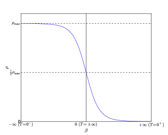
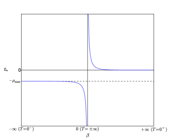
Figure 1: Energy density and pressure as functions of $\beta$ for a massless fermion with $\mu=0$ and $g\left(\epsilon\right)$ given by Eq. 3.

III Cosmology

We are finally ready to investigate the cosmological consequences of NAT. In this section we answer the question “How does a Universe at negative absolute temperature behave?”. In order to answer this, and motivated by our analysis so far, we first assume that a FLRW Universe is filled by a single perfect fluid in thermal equilibrium at NAT, and that this fluid is made up of fermions not subject to number conservation (which we shall refer to as temperons). The requirement of thermal equilibrium can probably be translated into a requirement for temperon-producing interactions to operate quickly compared to the Hubble time. We do not consider scenarios with number conservation and/or bosons because those entail additional (model-dependent) problems discussed in Appendix A. We further assume that at “low” energy scales these temperons should behave like all other known particles; i.e., like matter or radiation, depending on their mass.

New physics giving rise to the maximum energy cutoff required for NAT could produce new dynamics when many particles have energies close to the cutoff. However, to make progress, here we simply assume that general relativity still holds at the relevant macroscopic scales so that the dynamics of the NATive Universe will then be governed by the usual Friedmann equations

$$\begin{cases}3H^{2}=\rho\\ \dot{H}=-\frac{1}{2}\left(\rho+P\right),\end{cases}$$ (27)

where $\rho$ and $P$ will be calculated according to the process outlined in section II. The energy conservation equation,

$$\dot{\rho}=-3H\left(\rho+P\right),$$ (28)

can also be integrated to give a useful relation between the number of e-foldings the Universe has expanded (or contracted) and its initial and final energy densities:

$$N=-\frac{1}{3}\intop_{\rho_{i}}^{\rho_{f}}\frac{d\rho}{\rho+P}=-\frac{1}{3}\intop_{\rho_{i}}^{\rho_{f}}\frac{d\rho/\rho}{1+w},$$ (29)

where, as usual, $N\equiv\ln\frac{a_{f}}{a_{i}}$ and subscripts $i$ and $f$ denote “initial” and “final”, respectively.

In the first two subsections of this section we shall focus on analysing the background dynamics of two qualitatively different scenarios: NAT in expanding cosmologies (subsection III.1), and NAT in contracting cosmologies (subsection III.2). The remainder of this section will then be dedicated to discussing perturbation generation and the transition to a normal positive-temperature Universe.

III.1 NATive inflation

It can be easily seen from Eq. 28 that expanding cosmological solutions with negative temperature ($H>0$, $T<0$) have an attractor fixed point at $T=0^{-}$, corresponding to de Sitter expansion with $\rho=\rho_{\mathrm{max}}$ and $w=-1$. This has the interesting consequence that all expanding NATive Universes should tend towards a phase of exactly exponential inflation (although not necessarily reaching it) — therefore, if this limit is reached, we should expect $\rho_{\rm{max}}\lesssim\rm{10^{111}GeVm^{-3}}$ just from the fact that we have not seen primordial tensor modes.

Interestingly, unlike with most phantom inflation models (recall that Eq. 7 implies our expansion must either be phantom or exactly exponential), we do not have to worry about a Big Rip — a divergence of the scale factor in a finite interval of time Caldwell et al. (2003). This is simply because the energy density (and therefore $H$) here is bounded, so the evolution asymptotes to exponential expansion with constant density sufficiently quickly that the impact of the transient phantom period is small.

We start our quantitative analysis by showing that even if we begin very close to $T=-\infty$ we should expect to evolve towards the vicinity of $T=0^{-}$ extremely rapidly. If we are in the high $|T|$ regime where $|\beta\Lambda|\ll 1$ then, from Eqs. 25 and 29, the number of e-foldings between two densities while in this regime is

$$N\approx\frac{4/3}{\left(\ln 2\right)n_{\mathrm{max}}\left\langle\epsilon^{2}\right\rangle_{0}}\intop_{\rho_{i}}^{\rho_{f}}\left(\rho-\frac{1}{2}\rho_{\mathrm{max}}\right)d\rho\\ =\frac{2/3}{\left(\ln 2\right)n_{\mathrm{max}}\left\langle\epsilon^{2}\right\rangle_{0}}\left[\left(\rho_{f}-\frac{1}{2}\rho_{\mathrm{max}}\right)^{2}-\left(\rho_{i}-\frac{1}{2}\rho_{\mathrm{max}}\right)^{2}\right]\\ \approx\frac{\left\langle\epsilon^{2}\right\rangle_{0}}{n_{\mathrm{max}}}\frac{\beta_{f}^{2}-\beta_{i}^{2}}{24\ln 2},$$ (30)

where we have used

$$\beta\simeq\frac{4}{\left\langle\epsilon^{2}\right\rangle_{0}}\left(\frac{1}{2}\rho_{\mathrm{max}}-\rho\right).$$ (31)

In order to get some intuition regarding the order of magnitude we should expect from this $N$, we can assume the simple ansatz from Eq. 3 with $m=0$ (the order of magnitude should not change significantly as long as $m\ll\Lambda$) and find

$$\begin{array}[]{c}n_{\mathrm{max}}=\frac{g}{6\pi^{2}}\Lambda^{3}\\ \rho_{\mathrm{max}}=\frac{g}{8\pi^{2}}\Lambda^{4}\\ \left\langle\epsilon^{2}\right\rangle_{0}=\frac{g}{10\pi^{2}}\Lambda^{5}\end{array}$$ (32)

leading to

$$N=\mathcal{O}\left\{\frac{\left\langle\epsilon^{2}\right\rangle_{0}\beta_{f}^{2}}{n_{\mathrm{max}}}\right\}=\mathcal{O}\left\{\left(\beta_{f}\Lambda\right)^{2}\right\},$$ (33)

which is small by definition. Therefore, we should not expect to remain in this low-$\left|\beta\right|$ regime long enough for this epoch to significantly contribute to the total number of e-foldings.

Once $-\beta$ becomes comparable to $\Lambda$ it is harder to make predictions as the specific shape of $g\left(\epsilon\right)$ we are working with starts to make a difference. In other words, as $-\beta$ increases, we start needing more and more higher-order terms in the expansion in Eq. 25 which makes model-independent predictions impossible. Nevertheless, we know $\beta$ will have to keep evolving towards $-\infty$ and, sooner or later, we will be in the opposite limit where $-T\ll\Lambda$ and we can make use of the fact that holes should behave like either matter or radiation.

If holes behave like matter then

$$N=\frac{1}{3}\intop_{\rho_{i}}^{\rho_{f}}\frac{d\rho}{\rho_{\mathrm{max}}-\rho}=-\frac{1}{3}\intop_{\rho_{\mathrm{max}}-\rho_{i}}^{\rho_{\mathrm{max}}-\rho_{f}}\frac{dx}{x}\\ =\frac{1}{3}\ln\left[\frac{\rho_{\mathrm{max}}-\rho_{i}}{\rho_{\mathrm{max}}-\rho_{f}}\right]=\frac{1}{3}\ln\left[\frac{1+w_{i}^{-1}}{1+w_{f}^{-1}}\right]$$ (34)

where $w_{i}$ and $w_{f}$ are the initial and final $w$, respectively.

If instead holes behave like radiation then

$$N=\frac{1}{4}\intop_{\rho_{i}}^{\rho_{f}}\frac{d\rho}{\rho_{\mathrm{max}}-\rho}=\frac{1}{4}\ln\left[\frac{\rho_{\mathrm{max}}-\rho_{i}}{\rho_{\mathrm{max}}-\rho_{f}}\right]\\ =\frac{1}{4}\ln\left[\frac{\left(1+w_{i}\right)\left(1-3w_{f}\right)}{\left(1+w_{f}\right)\left(1-3w_{i}\right)}\right]$$ (35)

with essentially the same type of behaviour.

Notice that the density becomes exponentially close to $\rho_{\rm{max}}$ in just a few e-foldings, since Eq. (35) implies that

$$\rho_{f}=\rho_{\rm max}-(\rho_{\rm max}-\rho_{i})e^{-4N}$$ (36)

and $\rho_{i}=\mathcal{O}(\rho_{\rm max}/2)$. An analogous result holds for Eq. (34)).

In addition, note that if we compute the adiabatic sound speed

$$c_{s}^{2}\equiv\frac{\dot{P}}{\dot{\rho}},$$ (37)

we have

$$c_{s}^{2}=\begin{cases}1+4\frac{\ln 2}{\beta^{2}}\frac{n_{\mathrm{max}}}{\left\langle\epsilon^{2}\right\rangle_{0}}=\mathcal{O}\left\{\frac{1}{\left(\beta\Lambda\right)^{2}}\right\}\gg 1&\text{if}\ \left|\beta\Lambda\right|\ll 1\\ 0\qquad\text{if holes behave like matter}\\ \frac{1}{3}\qquad\text{if holes behave like radiation}\end{cases}$$ (38)

which shows that the sound speed only seems to be problematically large in the very high (negative) temperature regime which should only be valid at most during a very short time interval.

III.2 NATive bouncing Universe

Let us now turn our attention to a scenario where the Universe is contracting (i.e. $H<0$) and, normally, there would be a Big Crunch. For simplicity, we shall assume a spatially flat Universe (in the end we should expect the same type of qualitative evolution).

With an energy cut-off, a fermion component cannot be indefinitely compressed due to the Pauli exclusion principle. So either the fermions have to be destroyed as the universe collapses, or the contraction has to stop, preventing a Big Crunch (or there is new physics). If $w=-1$ exactly, so that $\rho=\rho_{\rm max}$ and contraction does not change the temperon energy density, we have the situation where fermions are destroyed at just the right rate for exponential contraction to continue indefinitely. However, in other cases we can hope for a bounce.

An expanding Universe tends towards $T=0^{\pm}$ (depending on the initial sign of $T$), but in the contracting case it should tend towards $\beta=0$. This is because the energy conservation equation forces $\dot{\rho}$ to have the same sign as $T$ and to be proportional to $-\frac{H}{\beta}$ once $\left|\beta\right|$ becomes sufficiently small. This causes $\rho$ to approach $\frac{1}{2}\rho_{\mathrm{max}}$, corresponding to $\beta=0$ (recall that $\rho+P$ must change sign at that point). At some point, then, the small $\beta$ approximation must become valid and we can follow the evolution of $H$ analytically. Note also that the dynamics of this system should not change appreciably even in the presence of other (normal) types of matter. This is because the NATive pressure singularity (which occurs for finite $a$) should dominate the Friedmann equations even if the energy density of temperons is subdominant (as for "normal" matter $\rho+P$ can only diverge when $a=0$).

Combining Eqs. 27 and 31, we can find a relation for the temperature as a function of $H^{2}$

$$\beta=\frac{2\rho_{\mathrm{max}}-12H^{2}}{\left\langle\epsilon^{2}\right\rangle_{0}}.$$ (39)

Using this we can write

$$\frac{dH}{dt}=-\frac{\ln 2}{2}n_{\mathrm{max}}\frac{\left\langle\epsilon^{2}\right\rangle_{0}}{2\rho_{\mathrm{max}}-12H^{2}},$$ (40)

which can be integrated to yield

$$-2\left(H^{3}-H_{i}^{3}\right)+\rho_{\mathrm{max}}\left(H-H_{i}\right)+\frac{\ln 2}{4}n_{\mathrm{max}}\left\langle\epsilon^{2}\right\rangle_{0}\left(t-t_{i}\right)\\ =0.$$ (41)

This encodes the evolution of $H\left(t\right)$ in a cubic equation; it has a well-known set of solutions, however it is easier to understand what happens next graphically.

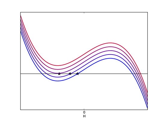
Figure 2: A graphic representation of Eq. 41 for increasing values of $t$ starting from $t_{i}$ (increasing from blue to red and bottom to top). The physical value of $H$ (when it exists) is indicated by a black star. The proportions between $\left\langle\epsilon^{2}\right\rangle_{0}$, $n_{\mathrm{max}}$, and $\rho_{\mathrm{max}}$ here correspond to those in Eqs. 32, however, it can be shown that a different scenario would look qualitatively the same.

From Eq. 41 we can see that $H$ at a given time is given by a root of a third order polynomial whose zeroth order coefficient is proportional to $t-t_{i}$ (see Fig. 2). At time $t=t_{i}$ there are three such roots, the physical solution corresponding to the middle one ($H=H_{i}$), which must be followed by continuity until the moment the temperature (and thus $\dot{H}$) becomes infinite (when $H^{2}=\frac{1}{6}\rho_{\mathrm{max}}$, meaning $\beta=0$). At that point, the root we were following disappears and there is no physically meaningful solution to Eq. 41 — which is not surprising since our formula for the pressure yields a division by zero at this point. Given that our equations are clearly invalid, we have to resort to physical arguments in order to know what must happen next. If we impose that the energy density is continuous and the thermal equilibrium assumption remains valid then $H$ must change sign discontinuously causing a bounce. However, since the pressure is discontinuous at that point, this is still not enough to determine the subsequent cosmological evolution. Both a scenario with $\dot{\beta}<0$ leading to the kind of NATive inflation discussed in subsection III.1 and a scenario with $\dot{\beta}>0$ leading immediately to a “normal” expanding Universe seem possible. The discontinuity in $H$ is likely to be an indication that our approach is not valid at the moment of the bounce. Nevertheless, it is not unreasonable to assume that thermal equilibrium should be restored relatively quickly after the bounce, leading to one of these two options.

As in the previous section, a contracting Universe can solve the horizon problem. In this case, the mechanism would be essentially the same as in most other bouncing Universe models: homogeneity would be brought about by a large positive pressure acting during a cosmological contraction. In order to solve this problem, bouncing cosmology models need to allow the quantity

$$\mathcal{N}_{H}\equiv\ln\left|aH\right|$$ (42)

to grow by a factor of order $60$ Lehners and Wilson-Ewing (2015). This seems to be achieved as long as the contraction starts at sufficiently small $H$. For example, assuming a matter or radiation dominated Universe at the beginning of the contraction,

$$\mathcal{N}_{H}\left(t\right)-\mathcal{N}_{H}\left(t_{i}\right)=\left(\frac{2}{3\left(1+w_{0}\right)}-1\right)\ln\left|\frac{H_{i}}{H\left(t\right)}\right|$$ (43)

where $w_{0}=1/3$ if radiation dominates. Since the left-hand side of Eq. 43 is always negative and $H^{2}$ is increasing during the contraction, it is always possible to get the right amount of contraction as long as the initial energy density is low enough.

If, instead, the Universe is initially at a very low negative temperature (let us assume, for simplicity, that holes behave like radiation), then

$$\mathcal{N}_{H}\left(t\right)-\mathcal{N}_{H}\left(t_{i}\right)=\frac{1}{4}\ln\left|\frac{\rho^{2}\left(t\right)\left(\rho_{\rm{max}}-\rho\left(t\right)\right)}{\rho^{2}_{i}\left(\rho_{\rm{max}}-\rho_{i}\right)}\right|$$ (44)

which can also be as large as needed provided that the initial hole density is small enough.

This would mean the NAT themselves would not really contribute to solving the horizon problem (though the extra positive pressure close to the bounce would help). In fact, NAT might not even occur in this scenario — it is enough for temperons to force a bounce in a model that would otherwise still solve these problems but end in a Big Crunch.

III.3 Perturbations

If NATive models are to be taken as realistic candidates to realise inflation or bouncing cosmologies, then a complete study of perturbation generation will be necessary. One of the main successes of standard inflation is how easy it is to write down a model which yields a nearly scale-invariant spectrum of scalar perturbations (which is in excellent agreement with CMB observations). One might think that the nearly-exponential expansion of a NAT fluid also would give a scale invariant spectrum of thermal fluctuations. However an exactly de Sitter phase produces no density fluctuations, and this limit is rapidly approached. Moreover, $\rho+P$ goes to zero sufficiently fast that curvature perturbations rapidly increase with time, leading to a blue spectrum until the de Sitter limit is saturated (see Appendix B for details). Thus pure NATive inflation cannot be a realistic model for the early Universe.

Instead we can consider a simple scenario with a spectator field that has negligible effect on the background evolution. Suppose that besides the temperons there exists a canonical scalar field $\sigma$ whose potential $V\left(\sigma\right)$ is much smaller than the temperon energy density (and does not interact with temperons). Since the background evolution is almost unchanged, the temperon density will still tend towards its maximum possible value with $P_{t}=-\rho_{t}=-\rho_{\mathrm{max}}$, and its contributions to the Friedmann equations will quickly become constant. The evolution is then the same as we would have for just a canonical scalar field with potential $V_{\rm eff}\left(\sigma\right)=V\left(\sigma\right)+\rho_{\mathrm{max}}$.

We can also look at the curvature perturbation produced in the same limit. Using the fact that the density perturbation due to temperons should tend to zero (since $\delta\rho_{t}=-\delta\rho_{\rm holes}$ and there are no holes at $T=0$), we have the interesting result that in the flat slicing

$$\zeta=-H\frac{\delta\rho}{\dot{\rho}}\rightarrow-H\frac{\delta\rho_{\sigma}}{\dot{\rho}_{\sigma}}\equiv\zeta_{\sigma},$$ (45)

where $\zeta_{\sigma}$ is the curvature perturbation we would get from the same scalar field (with potential $V_{\rm eff}\left(\sigma\right)=V\left(\sigma\right)+\rho_{\mathrm{max}}$). However, since the spectator field has (by construction) negligible density, this would not significantly contribute to an observable curvature perturbation if the dominant uniform temperon density somehow decays to give a radiation dominated universe. Instead, the spectator field fluctuation would either have to become dynamically important after temperon decay or somehow modulate the decay process. We discuss this further at the end of the next section.

III.4 Ending NATive inflation

The analysis so far has focused mostly on the basic cosmological implications of the possibility of domination by a temperon gas. Since an inflationary and a bouncing Universe both seem to be naturally realized in this sort of scenario, it is worth considering whether the transition from NATive inflation to a normal positive-temperature Universe — which we may call recooling, by analogy with reheating — can also happen naturally, giving rise to the standard Hot Big Bang cosmology.

The main difficulty in an expanding universe is that we have shown that a NAT fluid rapidly tends to the stable attractor solution with constant density $\rho=\rho_{\rm max}$, so on its own there is no dynamical evolution that could naturally set a timescale for recooling. However, as with reheating, the process of recooling to a universe dominated by familiar content must require some level of interaction with normal particles, however indirect, so it is possible that additional degrees of freedom could be responsible for ending NATive inflation.

Note that for $\rho>\frac{1}{2}\rho_{\rm max}$, the energy conservation equation for the temperons has $\dot{\rho_{t}}=-3H(\rho_{t}+P_{t})>0$ (with singular negative pressure term at the $\rho=\frac{1}{2}\rho_{\rm max}$ threshold between positive and negative temperatures), which prevents the temperon fluid from dynamically evolving to normal temperatures even if other components modify the background. The temperons also cannot be in equilibrium with normal matter (involving particles which do not admit negative temperatures), since equilibrium would be reached with both systems at a positive temperature, regardless of how small the additional positive-temperature system might be Romero-Rochín (2013). Any end to the NATive epoch must therefore involve an out of equilibrium process.

With this in mind, if we naively postulate that above a critical energy density temperons can interact with bosons slightly and even decay into bosons with some low probability, we should expect to recover a positive-temperature Universe some time after that critical energy density is reached. This whole process would necessarily take us away from equilibrium, so the formalism we have been using is no longer valid and it is not possible to make model-independent predictions. It seems plausible that it should be possible to get more e-foldings of inflation by forcing the temperon-photon interaction to be weaker, at the possible expense of fine tuning the interaction timescale to be close to the Hubble time. However we can see from Eqs. 34 and 35 that we would not get more than a few e-foldings of expansion in equilibrium unless the critical energy density is also fine-tuned to be extremely close to $\rho_{\mathrm{max}}$: if we wanted about $60$ e-foldings in this regime we would need $1-\frac{\rho_{c}}{\rho_{\mathrm{max}}}\lesssim 10^{-6}$. Note also that out of equilibrium the perturbation calculations from Appendix B would also not be applicable.

An added difficulty is how to calculate the effective pressure in a non-equilibrium setting. Unfortunately, this requires calculating the pressure from first principles, which is non-trivial and model-dependent - even in equilibrium. The mechanical pressure is usually given by the standard formula

$$P_{\rm{mech}}=\int_{m}^{\Lambda}\left(\frac{\epsilon^{2}-m^{2}}{3\epsilon}\right)g\left(\epsilon\right){\cal{N\left(\epsilon\right)}}d\epsilon.$$ (46)

However, we have been using the result of Eq. 15 (which assumes thermal equilibrium). These are not equivalent in the presence of a cutoff, and are only equivalent in the limit where $\Lambda\rightarrow\infty$ if $\beta>0$. This can be seen using integration by parts and assuming the ansatz in Eq. 3 as well as ${\cal{N}}=1/\left(e^{\beta\epsilon}+1\right)$, which yields

$$P=P_{{\rm mech}}+\frac{g}{2\pi^{2}}\frac{\left(\Lambda^{2}-m^{2}\right)^{3/2}}{3\beta}\ln\left(1+e^{-\beta\Lambda}\right)$$ (47)

for $\beta>0$. For negative temperatures the result instead follows Eq. (20).

It may seem a problem that Eq. (46) does not work for NAT (and in particular fails to even allow $P<0$). However, it was originally written down for ideal gases of classical particles and, at these high energy (and momentum) scales, close to the cut-off, there is no reason why that picture should still be valid. It is interesting to note that the pressure in the Friedmann equations should always coincide with that given by Eq. 15. This can be seen by noting that the first Friedmann equation is equivalent to the First Law of Thermodynamics in the case of adiabatic expansion/contraction.

Although we do not know how to calculate these "microscopic" pressures, some hints are given by the work of Paliathanasis et al. (2015), who did something similar for the case of a scalar field, finding that there was a negative correction to the pressure that made some normal inflation models become phantom. The main idea is to make use of the known fact Bojowald and Kempf (2012) that in these theories there is a significant deviation from the canonical commutation relation between the usual position and momentum operators, implying that the usual momentum operator is no longer the conjugate momentum of the position operator and invalidating the standard result. In principle, it should be possible to rewrite the Lagrangian in terms of the correct momentum operator and from that compute the corrections to the standard energy-momentum tensor due to this deformed algebra. This would then have the effect of adding corrections to both the pressure and the energy density, essentially solving our problem and enabling the accurate calculation of non-equilibrium pressures. The pursuit of this approach is left for future work. In principle, if it succeeds, it may help us understand what is required for a complete microphysical description of these fluids (at the Lagrangian level).

An alternative way to end NATive inflation would be to make use of a spectator field as described in Sec. III.3. A natural way to do this might be for the scalar field to precipitate the end of inflation, for example by having it decay into bosons which then interact with the temperons, ending inflation by full thermalisation. However, since the energy density of the spectator field should be subdominant, this would probably require a sharp feature in the potential to compensate the large Hubble damping from the background.

The curvature perturbation from the spectator field (Eq. 45) will have a nearly scale-invariant spectrum during temperon domination provided that it is light compared to the Hubble scale, but it does not automatically give rise to a significant amplitude of the curvature perturbation after recooling. Note that with two independent components $\zeta$ can change in time on superhorizon scales Wands et al. (2000). However, the temperon fluid should be very homogeneous, so the recooling surface would be determined by the scalar field perturbations $\delta\rho_{\sigma}$. The quasi-scale-invariant $\delta\rho_{\sigma}$ fluctuations can therefore convert into local variation in the recooling time, and hence a total curvature perturbation (i.e. essentially the same mechanism as the modulated reheating mechanism for multi-field inflation Dvali et al. (2004)). Non-Gaussianities could also be introduced at this stage analogously to similar scenarios in the context of inflation Byrnes and Choi (2010); Wands (2010). A specific model would be required to make quantitative predictions, in particular the perturbation amplitude is model dependent even if the fluctuation scale dependence is more generally preserved.

IV Conclusions

A fluid with negative temperature is an interesting effective macroscopic model for a component of the Universe, even without any compelling microphysical motivation. Regardless of the microphysics, the evolution of a NAT fluid dominated cosmology will be qualitatively the same and depend only on the initial value of the Hubble parameter (as summarised in table 1). It might be an attractive way to realise both inflation and bouncing cosmologies.

	$H<0$	$H>0$
$H^{2}<\frac{1}{6}\rho_{\mathrm{max}}$	NATive bouncing	standard cosmology
$H^{2}>\frac{1}{6}\rho_{\mathrm{max}}$	NATive bouncing	NATive inflation

Table 1: Fate of a temperon-dominated Universe depending on its initial conditions.

However, there are a number of significant problems with a naive application to cosmology:

• The physical plausibility of obtaining a maximum energy cutoff is unclear.

• For a NAT description to apply, the system must remain in equilibrium. In an expanding universe the NAT fluid has to be able to produce more particles rapidly as the universe expands (but no bosons), and any microphysical model would have to explain why this happens rather than simply rapidly decoupling and going out of equilibrium.

• In an expanding universe, the NAT component rapidly becomes indistinguishable from a cosmological constant at the background level, and it is therefore of limited interest for obtaining realistic dynamics that lead to the end of inflation.

• An additional component, such as a light scalar spectator field, would be required to produce an acceptable fluctuation spectrum.

• Any end of NATive inflation, or resolution of a bounce, requires non-equilibrium evolution that cannot be modelled in a model-independent way.
  

Nevertheless, it must be noted that, as long as the first assumption (about the existence of the energy cut off) holds, there will be interesting consequences even if the following problems cannot be overcome and our formalism cannot be used most of the time. Even if thermalization at a NAT turns out to be impossible, a universe with a cut-off would likely still lead to interesting dynamics (for example due to the pressure discontinuity at $T=+\infty$). Moreover, even if this component turns out to be unable to provide an acceptable explanation to horizon and flatness problems, it may still have interesting consequences in systems where it might be found if it exists — as in the interior of black holes.

The discussion of Appendix B suggests some ways in which acceptable fluctuations could be produced, though with additional ingredients and fine tuning such models have limited appeal.

Above all, we have shown that there are interesting cosmological consequences of NAT, and that it is possible that popular paradigms like inflation and bouncing cosmologies may be successfully realised in scenarios which are fundamentally different from the usual domination by simple scalar fields.

V Acknowledgements

We thank Mariusz Dąbrowski for bringing the work of Gonzalez-Diaz and Siguenza (2004) to our attention and Yi Wang for helpful comments on Chen et al. (2008). We also thank Carlos Martins, Daniel Passos, Daniela Saadeh, Frank Könnig, Henryk Nersisyan, Jonathan Braden, and Sam Young for fruitful discussions, insightful questions, and other useful references.

JV is supported by an STFC studentship, CB is supported by a Royal Society University Research Fellowship, and AL acknowledges support from the Science and Technology Facilities Council [grant number ST/L000652/1] and European Research Council under the European Union’s Seventh Framework Programme (FP/2007-2013) / ERC Grant Agreement No. [616170].

Appendix A Problems maintaining negative temperatures with number conservation and bosons

Let us start by assuming number conservation so that we can explore the kind of problems it causes. In an FLRW Universe with scale factor $a$ and Hubble parameter $H$, there will then be two equations governing the dynamics of these functions, the continuity equation

$$\dot{\rho}=-3H\left(\rho+P\right)$$ (48)

and the number conservation equation

$$\frac{\dot{n}}{n}=-3H.$$ (49)

Equivalently, one can make use of the symmetries in Eqs. 18, 19, and 20 to rewrite these for holes as

$$\dot{\rho_{h}}=-3H\left(\rho_{h}+P_{h}\right)$$ (50)

$$\dot{n_{h}}=3H\left(n_{\rm{max}}-n_{h}\right)$$ (51)

where the subscript $h$ denotes a quantity relative to holes (with $T_{h}=-T$). Note that the formal equivalence between Eqs. 48 and 50 is due to the fact that they both express the constraint that the entropy be conserved and entropy cannot distinguish between particles and holes (since it is purely combinatorial).

Suppose now that the Universe is filled with a temperon gas at NAT with $m\gg T_{h}$. If the very low-energy holes behave like normal (pressureless) matter then $\rho_{h}=mn_{h}$ and the previous equations are reduced to

$$\dot{\rho_{h}}=-3H\rho_{h}$$ (52)

$$\dot{\rho_{h}}=3Hmn_{\rm{max}}-3H\rho_{h}$$ (53)

which is an inconsistent system as long as $H\neq 0$. This would mean that in this situation equilibrium could not be maintained during the expansion.

Of course, this problem assumes a specific low-energy form of $g\left(\epsilon\right)$ and thus it can by no means be considered a refutation of the $\mu\neq 0$ case. Nevertheless, it is a difficulty that has to be taken into account and which raises questions about how model-independent (i.e., how independent of $g\left(\epsilon\right)$) such an analysis can be. In addition, if we just assume $g\left(\epsilon\right)$ is whatever is necessary to make this system of equations consistent, we have to live with the fact that there are possible situations in which the energy density will be increasing while the number density decreases (and vice-versa, if the Universe is contracting), since $\dot{\rho}/\dot{n}$ has the same sign as $\rho+P$ and $\rho$ is bounded whereas $P$ is not.

Moreover, it can be easily seen that, even accepting these odd behaviours, such a solution can never be consistent in all situations. For example, consider the case where temperons are massless fermions at $T=0^{-}$. In this situation, the energy density must be constant and equal to its maximum possible value, whereas the number density must vary according to $H$. This is clearly absurd as there is no way the system can be at $\rho=\rho_{\rm{max}}$ unless all states are filled.

Note that once we restrict ourselves to the study of cases without number conservation it becomes clear that we cannot use bosons: without number conservation, the energy of the system is no longer bounded from above, which makes NAT impossible.

Appendix B Thermal Perturbation Generation

A system in equilibrium will in general have thermal fluctuations. Here we consider the case where the Universe is dominated by temperons in thermal equilibrium, and calculate the density and curvature perturbations produced. We focus on the case where holes behave like radiation as $\beta\rightarrow-\infty$.

The main difference between perturbations here and in the standard inflationary scenario is that density perturbations here are produced due to classical thermal fluctuations rather than by quantum effects. The basic methodology used in this subsection is therefore essentially the same as the one used to work out thermal fluctuations in models such as chain inflation or warm inflation in the very weakly dissipative regime Chen et al. (2008).

B.1 Moments in position space

For a canonical thermal system with volume $V$, the $n$-th moment of the energy density distribution is given by

$$\left\langle\rho^{n}\right\rangle=\frac{\left\langle E^{n}\right\rangle}{V^{n}}=\frac{1}{Z}\left(-\frac{1}{V}\right)^{n}\frac{\partial^{n}Z}{\partial\beta^{n}}$$ (54)

where $Z$ is the partition function as given by Eq. 14 with $\mu=0$. Making the substitution $\partial_{\alpha}\equiv-V^{-1}\partial_{\beta}$, we can find the simple recursive relation

$$\left\langle\rho^{n+1}\right\rangle=\left[\left\langle\rho\right\rangle+\partial_{\alpha}\right]\left\langle\rho^{n}\right\rangle$$ (55)

which we can then use to find an analogous formula for the moments of $\delta\rho=\rho-\left\langle\rho\right\rangle$. Taking a derivative with respect to $\alpha$ of

$$\left\langle\left(\delta\rho\right)^{n}\right\rangle=\sum_{k=0}^{n}\frac{n!}{\left(n-k\right)!k!}\left(-\left\langle\rho\right\rangle\right)^{n-k}\left\langle\rho^{k}\right\rangle$$ (56)

and then making use of Eq. 55 yields

$$\left\langle\left(\delta\rho\right)^{n+1}\right\rangle=\partial_{\alpha}\left\langle\left(\delta\rho\right)^{n}\right\rangle+n\partial_{\alpha}\left\langle\rho\right\rangle\left\langle\left(\delta\rho\right)^{n-1}\right\rangle.$$ (57)

Eq. 57 has the interesting feature of separating contributions from even and odd momenta in the right-hand side. Because of it, and since $\left\langle\delta\rho\right\rangle=0$, if we assume that $\left\langle\left(\delta\rho\right)^{3}\right\rangle=\partial_{\alpha}^{2}\left\langle\rho\right\rangle=0$ then (as can be easily checked by induction) every odd moment has to be zero and $\left\langle\left(\delta\rho\right)^{2n}\right\rangle=\left(2n-1\right)!!\left\langle\left(\delta\rho\right)^{2}\right\rangle^{n}$, corresponding to exactly Gaussian perturbations whose statistics depend only on the size of the thermal system $V$ (and not on $\beta$). In other words, in this scenario Gaussianity is equivalent to the third moment of $\delta\rho$ being null and to the second (and indeed every even) moment being independent of $\beta$. Since

$$\left\langle\left(\delta\rho\right)^{3}\right\rangle=\partial_{\alpha}^{2}\left\langle\rho\right\rangle=\frac{1}{V^{2}}\intop g\left(\epsilon\right)\epsilon^{3}\left[\frac{e^{2\beta\epsilon}-e^{\beta\epsilon}}{\left(e^{\beta\epsilon}+1\right)^{3}}\right]d\epsilon,$$ (58)

then density perturbations must always be exactly Gaussian for $\beta=0$ (at the bounce) and for the attractors $\beta=\pm\infty$. This exact Gaussianity at the attractors, however, is misleading since it corresponds to a limit in which density perturbations must vanish — recall that from Eq. 18 we have $\delta\rho=-\delta\rho_{\rm holes}$ (where the temperature of holes is symmetric to that of particles) and $\delta\rho$ has to be zero for $T=0^{+}$ since at that temperature the density itself is zero. We should thus look at the relevant perturbation, the curvature perturbation, which can be written in terms of the density perturbation in the zero curvature frame (in which the previous calculations make sense as the shape of the “box” is not perturbed) as

$$\zeta=\frac{1}{3}\frac{\delta\rho}{\left\langle\rho\right\rangle+\left\langle P\right\rangle}.$$ (59)

In the case of a bounce, this also shows that even the Gaussian perturbations are less interesting than one might think, since despite the numerator being non-zero the denominator diverges, making the relevant curvature perturbation negligible.

The variance of the curvature perturbation can now be found to be given by

$$\left\langle\zeta^{2}\right\rangle=\frac{1}{9}\frac{\left\langle\delta\rho^{2}\right\rangle}{\left(\rho+P\right)^{2}}=-\frac{1}{9V}\frac{\partial_{\beta}\rho}{\left(\rho+P\right)^{2}},$$ (60)

where for simplicity we are using $\rho$ and $P$ interchangeably with their averages.

The most interesting limit for Eq. 60 is when $\beta\rightarrow-\infty$ as the spacetime then tends towards unperturbed de Sitter, yet the curvature perturbation does not necessarily tend to zero as the denominator in the right-hand side also goes to zero in this limit. For example, if holes behave like radiation, the denominator vanishes at a faster rate than the numerator, causing $\zeta$ to diverge as (see table 2 for a breakdown of the relevant terms in Eq. 60 in this limit)

$$\left\langle\zeta^{2}\right\rangle=\left(\frac{15}{7\pi^{2}g}\right)^{1/4}\frac{\left(\rho_{\mathrm{max}}-\rho\right)^{-3/4}}{2V}.$$ (61)

	$\rho_{h}=\rho_{\mathrm{max}}-\rho$	$a_{\star}=aV_{0}^{-1/3}$
$\rho+P$	$-\frac{4}{3}\rho_{h}$	$-\frac{4}{3}a_{\star}^{-4}$
$\beta$	-$\left(\frac{7\pi^{2}}{240}\frac{g}{\rho_{h}}\right)^{1/4}$	$-\left(\frac{7\pi^{2}}{240}g\right)^{1/4}a_{\star}$
$\left\langle\left(\delta\rho\right)^{2}\right\rangle$	$\frac{8}{V}\left(\frac{15}{7\pi^{2}g}\right)^{1/4}\rho_{h}^{5/4}$	$\frac{8}{V}\left(\frac{15}{7\pi^{2}g}\right)^{1/4}a_{\star}^{-5}$
$\left\langle\zeta^{2}\right\rangle$	$\frac{1}{2V}\left(\frac{15}{7\pi^{2}g}\right)^{1/4}\rho_{h}^{-3/4}$	$\frac{1}{2V}\left(\frac{15}{7\pi^{2}g}\right)^{1/4}a_{\star}^{3}$

Table 2: Summary of relevant quantities as functions of hole energy density, $\rho_{h}$, and rescaled scale factor, $a_{\star}=\rho_{h}^{-1/4}$, when holes behave like radiation. The row for $\beta$ comes from applying the standard result for the fermion energy density to $\rho_{h}$. $V_{0}$ is the integration constant used later in Eq. 71.

B.2 The thermal power spectrum

In order to turn the results from the previous section into predictions for the power spectrum, we must introduce a couple of mathematical objects and endure some integral manipulations.

Let us start by considering the average density fluctuation in the vicinity of a point,

$$\delta\rho_{\mathbf{x_{0}}}\left(r\right)\equiv\frac{1}{V_{r}}\intop_{S_{r,\mathrm{x_{0}}}}d^{3}{\bf x}\delta\rho\left(\mathbf{x}\right)=\frac{1}{V_{r}}\intop_{S_{r}}d^{3}{\bf x}\delta\rho\left(\mathbf{x_{0}+x}\right)\\ =\frac{1}{V_{r}}\intop\frac{d^{3}{\bf k}}{\left(2\pi\right)^{3/2}}\delta\rho_{{\bf k}}\intop_{S_{r}}d^{3}{\bf x}e^{i{\bf k\cdot\left(x_{0}+x\right)}},$$ (62)

where $S_{r,{\bf x_{0}}}$ is the sphere of comoving radius $r$ centred around $\mathbf{x_{0}}$, $S_{r}=S_{r,{\bf 0}}$, and $V_{r}=\frac{4}{3}\pi r^{3}$.

We can define the average power of this quantity as

$$\overline{\delta\rho}^{2}\left(r\right)\equiv\lim_{R\rightarrow\infty}\frac{1}{V_{R}}\intop_{S_{R}}d^{3}{\bf x_{0}}\left|\delta\rho_{{\bf x_{0}}}\left(r\right)\right|^{2}$$ (63)

which can be rewritten as

$$\overline{\delta\rho}^{2}\left(r\right)=\lim_{R\rightarrow\infty}\intop\frac{d^{3}{\bf k}}{\left(2\pi\right)^{3/2}}\intop\frac{d^{3}{\bf k}^{\prime}}{\left(2\pi\right)^{3/2}}\\ \times\delta\rho_{{\bf k}}\delta\rho_{{\bf k}^{\prime}}W_{r}\left(k\right)W_{r}\left(k^{\prime}\right)W_{R}\left(\left\|{\bf k+k^{\prime}}\right\|\right),$$ (64)

where we have used the window function defined as

$$W_{r}\left(k\right)\equiv\frac{1}{V_{r}}\intop_{S_{r}}d^{3}{\bf x}e^{i{\bf x\cdot k}}=3\frac{\sin\left(kr\right)-kr\cos\left(kr\right)}{\left(kr\right)^{3}}.$$ (65)

Taking the expected value on both sides and using the definition $\left\langle\delta\rho_{{\bf k}}\delta\rho_{{\bf k^{\prime}}}\right\rangle\equiv\delta\left({\bf k+k^{\prime}}\right)P_{\delta\rho}\left(k\right)$ then yields

$$\left\langle\overline{\delta\rho}^{2}\left(r\right)\right\rangle=\intop\frac{d^{3}{\bf k}}{\left(2\pi\right)^{3}}\left|W_{r}\left(k\right)\right|^{2}P_{\delta\rho}\left(k\right).$$ (66)

Alternatively, using the usual definition of the power spectrum ${\cal P}\left(k\right)=k^{3}P\left(k\right)/\left(2\pi^{2}\right)$, this is

$$\left\langle\overline{\delta\rho}^{2}\left(r\right)\right\rangle=\intop_{0}^{\infty}\frac{dk}{k}\left|W_{r}\left(k\right)\right|^{2}\mathcal{P}_{\delta\rho}\left(k\right).$$ (67)

Provided that $P_{\delta\rho}\left(k\right)$ doesn’t diverge faster than $k^{-3}$ as $k\rightarrow 0$, the integral in Eq. 66 is dominated by $k\sim r^{-1}$ and Mukhanov et al. (1992)

$$P_{\delta\rho}\left(k\right)\sim\frac{\left(2\pi\right)^{3}}{k^{3}}\left\langle\overline{\delta\rho}^{2}\left(k^{-1}\right)\right\rangle.$$ (68)

Assuming there is a thermal horizon, $L_{\rm th}$, corresponding to the physical distance beyond which there can be no thermal correlation, the actual observed density power spectrum can be calculated from Eq. 68 evaluated around thermal horizon exit, when $k\sim a/L_{\rm th}$. Using $\left\langle\overline{\delta\rho}^{2}\left(L/a\right)\right\rangle=\left\langle\left(\delta\rho\right)^{2}\right\rangle_{V_{\rm th}}$ we conclude that

$$\left\langle\overline{\delta\rho}^{2}\left(r\right)\right\rangle=\left\langle\left(\delta\rho\right)^{2}\right\rangle_{V=a^{3}V_{r}},$$ (69)

and hence

$$P_{\zeta}\left(k\sim a/L_{\rm th}\right)\sim\frac{\left(2\pi\right)^{3}L_{\rm th}^{3}}{9a^{3}\left(\rho+P\right)^{2}}\left\langle\delta\rho^{2}\right\rangle_{V=\frac{4\pi}{3}L_{\rm th}^{3}}\\ \sim-\frac{\left(2\pi\right)^{3}}{12a^{3}}\frac{\partial_{\beta}\rho}{\left(\rho+P\right)^{2}},$$ (70)

where everything is evaluated around thermal horizon crossing.

If we further assume holes behave like radiation, we can use this together with equation 61 and immediately get

$$P_{\zeta}\left(k\right)\sim\frac{3}{8}\left(\frac{15}{7\pi^{6}g}\right)^{1/4}\frac{\left(2\pi\right)^{3}}{V_{0}},$$ (71)

where $V_{0}\equiv a^{3}\left(\rho_{\mathrm{max}}-\rho\right)^{3/4}$ is a constant thanks to Eq. 35. Note that this corresponds to a white noise spectrum with $n_{s}=4$.

If the NAT model were to describe a realistic cosmology, we would need the power spectrum to be (approximately) scale-invariant, at least in the attractor $\beta\rightarrow-\infty$ limit. Unfortunately, we can show that is not necessarily possible even if we allow drastic departures from Eq. 3. From Eq. 68 it is clear that the spectrum will be scale invariant if and only if $\left\langle\overline{\delta\rho}^{2}\left(k^{-1}\right)\right\rangle$ is independent of $k$. In other words, the power spectrum can be written as

$${\cal P}_{\zeta}\left(k\right)\sim-\frac{4\pi}{9V}\frac{\partial_{\beta}\rho}{\left(\rho+P\right)^{2}},$$ (72)

which is a constant if and only if

$$\partial_{k}\left(V^{-1}\frac{\partial_{\beta}\rho}{\left(\rho+P\right)^{2}}\right)=0.$$ (73)

Assuming, as before, that $V\propto L_{\rm th}^{3}=\text{const}$, this can be rewritten as

$$\frac{\partial_{\beta}\rho^{-1}}{\left(1+w\right)^{2}}=\text{const}.$$ (74)

Note that if $w_{h}$ is the equation of state of holes then Eqs. 18 and 21 yield $\rho+P=-\rho_{h}-P_{h}$ (where the subscript $h$ once again denotes holes) and thus Eq. 74 is equivalent to

$$\frac{\partial_{\beta_{h}}\rho_{h}^{-1}}{\left(1+w_{h}\right)^{2}}=\text{const}.$$ (75)

Consequently, if $w_{h}=\text{const}$ then in this large $\beta>0$ limit

$$\rho=\frac{1}{A+B\beta},$$ (76)

where $A$ and $B$ are positive constants of integration — they have to be positive because $B$ is related to the power spectrum by ${\cal P}_{\zeta}\left(k\right)\sim\frac{4\pi}{9V}\frac{B}{\left(1+w_{h}\right)^{2}}$. If we now equate the right-hand sides of Eq. 9 and Eq. 76 and take a derivative with respect to $T$ at $T=0^{+}$ we get

$$\lim_{\beta\rightarrow\infty}\beta^{2}\int\frac{g\left(\epsilon\right)\epsilon^{2}e^{\beta\epsilon}}{\left(e^{\beta\epsilon}+1\right)^{2}}d\epsilon=1$$ (77)

which is absurd since the left-hand side should be zero as long as there is a finite total number of one-particle states.

References

- Braun et al. (2013) S. Braun, J. P. Ronzheimer, M. Schreiber, S. S. Hodgman, T. Rom, I. Bloch, and U. Schneider, “Negative absolute temperature for motional degrees of freedom,” Science 339, 52–55 (2013), http://www.sciencemag.org/content/339/6115/52.full.pdf .
- Dunkel and Hilbert (2014) Jorn Dunkel and Stefan Hilbert, “Consistent thermostatistics forbids negative absolute temperatures,” Nature Physics 10, 67–72 (2014).
- Schneider et al. (2014) U. Schneider, S. Mandt, A. Rapp, S. Braun, H. Weimer, I. Bloch, and A. Rosch, “Comment on ”Consistent thermostatistics forbids negative absolute temperatures”,” ArXiv e-prints (2014), arXiv:1407.4127 [cond-mat.quant-gas] .
- Frenkel and Warren (2015) D. Frenkel and P. B. Warren, “Gibbs, Boltzmann, and negative temperatures,” American Journal of Physics 83, 163–170 (2015), arXiv:1403.4299 [cond-mat.stat-mech] .
- Dunkel and Hilbert (2014) J. Dunkel and S. Hilbert, “Reply to Schneider et al. [arXiv:1407.4127v1],” ArXiv e-prints (2014), arXiv:1408.5392 [cond-mat.stat-mech] .
- Ferrari (2015) L. Ferrari, “Boltzmann vs Gibbs: a finite-size match,” ArXiv e-prints (2015), arXiv:1501.04566 [cond-mat.stat-mech] .
- Hilbert et al. (2014) S. Hilbert, P. Hänggi, and J. Dunkel, “Thermodynamic laws in isolated systems,” Phys. Rev. E 90, 062116 (2014), arXiv:1408.5382 [cond-mat.stat-mech] .
- Gagliardi and Pecchia (2015) A. Gagliardi and A. Pecchia, “How to reconcile Information theory and Gibbs-Herz entropy for inverted populated systems,” ArXiv e-prints (2015), arXiv:1503.02824 [physics.class-ph] .
- Buonsante et al. (2016) P. Buonsante, R. Franzosi, and A. Smerzi, “On the dispute between Boltzmann and Gibbs entropy,” ArXiv e-prints (2016), arXiv:1601.01509 [cond-mat.stat-mech] .
- Purcell and Pound (1951) E. M. Purcell and R. V. Pound, “A nuclear spin system at negative temperature,” Phys. Rev. 81, 279–280 (1951).
- Ramsey (1956) Norman F. Ramsey, “Thermodynamics and statistical mechanics at negative absolute temperatures,” Phys. Rev. 103, 20–28 (1956).
- (12) G. L. Eyink and H. Spohn, “Negative-temperature states and large-scale, long-lived vortices in two-dimensional turbulence,” Journal of Statistical Physics 70, 833–886.
- Brevik and Gr n (2013) Iver Brevik and yvind Gr n, “Universe Models with Negative Bulk Viscosity,” Astrophys. Space Sci. 347, 399–404 (2013), arXiv:1306.5634 [gr-qc] .
- Gonzalez-Diaz and Siguenza (2004) Pedro F. Gonzalez-Diaz and Carmen L. Siguenza, “Phantom thermodynamics,” Nucl. Phys. B697, 363–386 (2004), arXiv:astro-ph/0407421 [astro-ph] .
- Myung (2009) Yun Soo Myung, “Does phantom thermodynamics exist?” Phys. Lett. B671, 216–218 (2009), arXiv:0810.4385 [gr-qc] .
- Lima and Pereira (2008) J. A. S. Lima and S. H. Pereira, “Chemical Potential and the Nature of the Dark Energy: The case of phantom,” Phys. Rev. D78, 083504 (2008), arXiv:0801.0323 [astro-ph] .
- Pereira and Lima (2008) S. H. Pereira and J. A. S. Lima, “On Phantom Thermodynamics,” Phys. Lett. B669, 266–270 (2008), arXiv:0806.0682 [gr-qc] .
- Pacheco (2008) J. A. de Freitas Pacheco, “Comments on Accretion of Phantom Fields by Black Holes and the Generalized Second Law,” (2008), arXiv:0808.1863 [astro-ph] .
- Silva et al. (2013) H. H. B. Silva, R. Silva, R. S. Gon alves, Zong-Hong Zhu, and J. S. Alcaniz, “General treatment for dark energy thermodynamics,” Phys. Rev. D88, 127302 (2013), arXiv:1312.3216 [astro-ph.CO] .
- Saridakis et al. (2009) Emmanuel N. Saridakis, Pedro F. Gonzalez-Diaz, and Carmen L. Siguenza, “Unified dark energy thermodynamics: varying w and the -1-crossing,” Class. Quant. Grav. 26, 165003 (2009), arXiv:0901.1213 [astro-ph.CO] .
- Hossenfelder (2013) Sabine Hossenfelder, “Minimal Length Scale Scenarios for Quantum Gravity,” Living Rev. Rel. 16, 2 (2013), arXiv:1203.6191 [gr-qc] .
- Garay (1995) Luis J. Garay, “Quantum gravity and minimum length,” Int. J. Mod. Phys. A10, 145–166 (1995), arXiv:gr-qc/9403008 [gr-qc] .
- Blundell and Blundell (2006) S. Blundell and K.M. Blundell, Concepts in Thermal Physics (Oxford University Press, 2006).
- Caldwell et al. (2003) Robert R. Caldwell, Marc Kamionkowski, and Nevin N. Weinberg, “Phantom energy and cosmic doomsday,” Phys. Rev. Lett. 91, 071301 (2003), arXiv:astro-ph/0302506 [astro-ph] .
- Lehners and Wilson-Ewing (2015) Jean-Luc Lehners and Edward Wilson-Ewing, “Running of the scalar spectral index in bouncing cosmologies,” (2015), arXiv:1507.08112 [astro-ph.CO] .
- Romero-Rochín (2013) V. Romero-Rochín, “Nonexistence of equilibrium states at absolute negative temperatures,” Phys. Rev. E 88, 022144 (2013), arXiv:1301.0852 [cond-mat.stat-mech] .
- Paliathanasis et al. (2015) Andronikos Paliathanasis, Supriya Pan, and Souvik Pramanik, “Scalar field cosmology modified by the Generalized Uncertainty Principle,” (2015), arXiv:1508.06543 [gr-qc] .
- Bojowald and Kempf (2012) Martin Bojowald and Achim Kempf, “Generalized uncertainty principles and localization of a particle in discrete space,” Phys. Rev. D86, 085017 (2012), arXiv:1112.0994 [hep-th] .
- Wands et al. (2000) David Wands, Karim A. Malik, David H. Lyth, and Andrew R. Liddle, “A New approach to the evolution of cosmological perturbations on large scales,” Phys. Rev. D62, 043527 (2000), arXiv:astro-ph/0003278 [astro-ph] .
- Dvali et al. (2004) Gia Dvali, Andrei Gruzinov, and Matias Zaldarriaga, “A new mechanism for generating density perturbations from inflation,” Phys. Rev. D69, 023505 (2004), arXiv:astro-ph/0303591 [astro-ph] .
- Byrnes and Choi (2010) Christian T. Byrnes and Ki-Young Choi, “Review of local non-Gaussianity from multi-field inflation,” Adv. Astron. 2010, 724525 (2010), arXiv:1002.3110 [astro-ph.CO] .
- Wands (2010) David Wands, “Local non-Gaussianity from inflation,” Class. Quant. Grav. 27, 124002 (2010), arXiv:1004.0818 [astro-ph.CO] .
- Chen et al. (2008) Bin Chen, Yi Wang, and Wei Xue, “Inflationary nonGaussianity from thermal fluctuations,” JCAP 0805, 014 (2008), arXiv:0712.2345 [hep-th] .
- Mukhanov et al. (1992) V.F. Mukhanov, H.A. Feldman, and R.H. Brandenberger, “Theory of cosmological perturbations,” Physics Reports 215, 203 – 333 (1992).