An Autonomous Dynamical System Captures all LCSs in Three-Dimensional Unsteady Flows

Abstract

Lagrangian coherent structures (LCSs) are material surfaces that shape finite-time tracer patterns in flows with arbitrary time dependence. Depending on their deformation properties, elliptic and hyperbolic LCSs have been identified from different variational principles, solving different equations. Here we observe that, in three dimensions, initial positions of all variational LCSs are invariant manifolds of the same autonomous dynamical system, generated by the intermediate eigenvector field, $\xi_{2}(x_{0})$, of the Cauchy-Green strain tensor. This $\xi_{2}$-system allows for the detection of LCSs in any unsteady flow by classic methods, such as Poincaré maps, developed for autonomous dynamical systems. As examples, we consider both steady and time-aperiodic flows, and use their dual $\xi_{2}$-system to uncover both hyperbolic and elliptic LCSs from a single computation.

Tracer patterns, such as the funnel of a tornado, suggest the emergence of coherence even in complex unsteady flows. As a mathematical tool for analyzing the dynamics behind time-evolving tracer patterns, Lagrangian coherent structures (LCSs) represent a generalization of classic invariant manifolds to non-autonomous systems. In three dimensions, the available LCS types (hyperbolic and elliptic) have been identified from different principles. Here we observe that for any unsteady flow in three dimensions, there is a single autonomous dynamical system capturing all LCSs. Specifically, this dynamical system is given by the intermediate eigenvector field of the Cauchy-Green strain tensor. Our observation enables the identification of LCSs in any unsteady flow by standard numerical methods for autonomous systems.

I Introduction

Lagrangian coherent structures (LCSs, (Haller2015, )) are exceptional surfaces of trajectories that shape tracer patterns in unsteady flows over finite time intervals of interest. By their sustained coherence, LCSs are observed as barriers to transport. In autonomous or time-periodic dynamical systems, classic codimension-one invariant manifolds play a similar role (e.g., Komolgorov-Arnold-Moser (KAM) tori (Arnold1989specific, )). In the time-aperiodic and finite-time setting, this role is taken over by LCSs as codimension-one invariant manifolds (material surfaces) in the extended phase space.

Material surfaces are abundant, yet most impose no observable coherence. LCSs are distinguished material surfaces that have exceptional impact on nearby material surfaces. Since various distinct mechanisms producing such impact are known (Haller2015, ), no unique mathematical approach has been available to locate all the LCSs in a given flow. Instead, separate mathematical methods and computational algorithms exist for the three main LCS types: hyperbolic LCSs as generalizations of stable and unstable manifolds (Haller2011a, ; Blazevski2014, ); elliptic LCSs as generalizations of invariant tori (Haller2013, ; Blazevski2014, ; Oettinger2016, ); and, in two dimensions, parabolic LCSs as generalized jet cores (Farazmand2014a, ).

Several works (Haller2011a, ; Haller2013, ; Farazmand2014a, ; Blazevski2014, ; Oettinger2016, ) have implemented properties that distinguish LCSs from generic material surfaces by requiring the LCSs to yield a critical value for a relevant quantity of material deformation. The criticality requirement defining, for instance, repelling hyperbolic LCSs (generalized stable manifolds) is that these material surfaces exert locally strongest repulsion (Blazevski2014, ). Elliptic LCSs in two dimensions, on the other hand, can be obtained as stationary curves of an averaged stretching functional (Haller2013, ). For the remaining LCS types in two and three dimensions, similar variational theories are available (Haller2011a, ; Farazmand2014a, ; Blazevski2014, ; Oettinger2016, ).

All the variational LCS theories (Haller2011a, ; Haller2013, ; Farazmand2014a, ; Blazevski2014, ; Oettinger2016, ) provide particular direction fields to which initial LCS positions must be either tangent (in two dimensions) or normal (in three dimensions). Later LCS positions can then be constructed by forward or backward advection under the flow map.

In two dimensions, LCSs are simply material curves (Haller2015, ; Haller2013, ; Farazmand2014a, ). Initial LCS positions can thus be identified by computing integral curves of (time-independent) direction fields defined in the two-dimensional phase space. Obtaining initial-time LCS surfaces in three dimensions (Blazevski2014, ; Oettinger2016, ), on the other hand, is significantly more complicated: One has to construct entire surfaces perpendicular to a given three-dimensional direction field. The presently available approach to extracting these surfaces is to sample the flow domain using two-dimensional reference planes, and then, within each plane, integrate direction fields that are perpendicular to the imposed LCS normal field. This procedure typically yields a high number of integral curves, which are candidates for intersection curves between unknown LCSs and the respective slice of the flow domain. As a second step, from this large collection of candidate curves, one has to identify smaller families of curves that can be interpolated into surfaces. Moreover, since the normal fields depend on the type of LCS, one has to repeat this complicated analysis for each LCS type (Blazevski2014, ; Oettinger2016, ).

Here we observe that initial positions of all available variational LCSs in three dimensions share a common tangent vector field: the intermediate eigenvector field, $\xi_{2}(x_{0})$, of the right Cauchy-Green strain tensor. This allows us to seek all LCSs in three dimensions as invariant manifolds of the autonomous dynamical system generated by the $\xi_{2}$-field. The evolution of the $\xi_{2}$-system takes place in the initial configuration of the underlying non-autonomous system, but contains averaged information about the non-autonomous flow. The autonomous $\xi_{2}$-system is hence dual to the original unsteady flow. Equivalently, LCS final positions are invariant manifolds of the intermediate eigenvector field, $\eta_{2}(x_{1})$, of the left Cauchy-Green strain tensor.

Instead of identifying LCSs in three dimensions from various two-dimensional direction fields (Blazevski2014, ; Oettinger2016, ), we therefore need to consider only a single three-dimensional direction field. We then locate LCSs by familiar numerical methods developed for autonomous dynamical systems.

II Set-up for Lagrangian coherent structures in 3D

Here we briefly review the mathematical foundations for Lagrangian coherent structures in three dimensions (Haller2015, ). We consider ordinary differential equations of the form

$$\dot{x}=u(x,t),\quad x\in U,\quad t\in I,$$ (1)

where $U$ is a domain in the Euclidean space $\mathbb{R}^{3}$; $I$ is a time interval; $u$ is a smooth mapping from the extended phase space $U\times I$ to $\mathbb{R}^{3}$. The setting in (1) includes time-aperiodic, non-autonomous dynamical systems for which asymptotic limits are undefined.

We consider a finite time interval $[t_{0},t_{1}]\subset I$ and denote a trajectory of (1) passing through a point $x_{0}$ at time $t_{0}$ by $x(t;t_{0},x_{0})$. For points $x_{0}$ where the trajectory $x(t;t_{0},x_{0})$ is defined for all times $t\in[t_{0},t_{1}]$, we introduce the flow map $F_{t_{0}}^{t}(x_{0}):=x(t;\,t_{0},\,x_{0}).$ Denoting the support of $F_{t_{0}}^{t}$ by $D$, the flow map is a diffeomorphism onto its image $F_{t_{0}}^{t}(D)$. Hence the inverse $\left(F_{t_{0}}^{t}\right)^{-1}$ exists, and, in particular, $\left(F_{t_{0}}^{t}\right)^{-1}=F_{t}^{t_{0}}.$

Definition 1 (Material surface).

Consider a set of initial positions forming a two-dimensional surface $\text{$\mathcal{M}$}(t_{0})$ at time $t_{0}$ in $U$. Its time-$t$ image, $\text{$\mathcal{M}$}(t)$, is obtained under the flow map as

$$\text{$\mathcal{M}$}(t)=\text{$F{}_{t_{0}}^{t}(\mathcal{M}$}(t_{0})).$$ (2)

The union of all time-$t$ images, $\cup_{t\in[t_{0},t_{1}]}\text{$\mathcal{M}$}(t)$, is a hypersurface in the extended phase space $U\times I$, called a material surface. Unless we consider a specific time-$t^{*}$ image $\text{$\mathcal{M}$}(t^{*})$ by fixing time to a certain value $t^{*}\in[t_{0},t_{1}]$, we refer to the entire material surface simply by the notation $\text{$\mathcal{M}$}(t)$.

Any material surface is an invariant manifold in the extended phase space $U\times I$ and, hence, cannot be crossed by integral curves $(x(t;t_{0},x_{0}),t)$. Only special material surfaces, however, create coherence in the phase space $U$ and hence act as observable transport barriers. Such material surfaces are generally called Lagrangian coherent structures (LCSs).

Quantifying material coherence in a general non-autonomous system requires considering (1) for a fixed time interval $[t_{0},t_{1}]$. This reflects the observation that coherent structures in truly unsteady flows are generally transient. (See also (Haller2015, ).) Accordingly, any LCS is defined with respect to the fixed time interval $[t_{0},t_{1}]$. (Thus, in applications where multiple time intervals $[t_{0},t_{1}]$ are relevant, the LCSs need to be determined separately for each time interval.)

Viewed in the phase space $U$, LCSs are time-dependent surfaces, even if the underlying dynamical system (1) is autonomous. LCS positions at different times are related via (2).

In applications, even if the flow map $F_{t_{0}}^{t}$ is available for all $t\in[t_{0},t_{1}]$, it remains challenging to detect and parametrize all the a priori unknown LCSs. This, fortunately, need not be done in the extended phase space: Since the flow map applied to any LCS position $\text{$\mathcal{M}$}(t^{*})$ uniquely generates any required time-$t$ image $\text{$\mathcal{M}$}(t)$, we can fix the time $t^{*}$ to an arbitrary value in $[t_{0},t_{1}]$ and parametrize $\text{$\mathcal{M}$}(t^{*})$ in the phase space $U$. For simplicity, we generally choose $t^{*}=t_{0}$. (For attracting hyperbolic LCSs, however, it is advantageous to parametrize $\text{$\mathcal{M}$}(t_{1})$ instead of $\text{$\mathcal{M}$}(t_{0})$, see Sec. V.3.). The difficulty remains in that almost any conceivable surface from the domain $D$ evolves incoherently under the flow, and hence does not define an LCS $\text{$\mathcal{M}$}(t)$ (cf. Fig. 1). We therefore need additional properties that, for any time-aperiodic flow, distinguish LCSs from generic material surfaces.

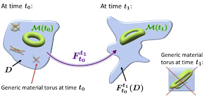
Figure 1: Schematic of an elliptic LCS $\text{$\mathcal{M}$}(t)$, obtained as a toroidal surface $\text{$\mathcal{M}$}(t_{0})$ in the flow domain $D$ at time $t_{0}$. Up to rotations and translations, the time-$t_{1}$ image, $\text{$\mathcal{M}$}(t_{1})$, is only moderately deformed relative to $\text{$\mathcal{M}$}(t_{0})$ and does not display additional features, such as filaments. (In the context of fluid dynamics, such an LCS could capture a coherently evolving vortex ring in a three-dimensional unsteady flow.) Generic tori in $D$, on the other hand, are expected to evolve incoherently under the flow $F_{t_{0}}^{t_{1}}$ and thus do not yield LCSs.

III Review of variational approaches to Lagrangian coherent structures in 3D

Within the general class of three-dimensional flows with arbitrary time dependence (1), several types of material surfaces can be viewed as coherently evolving. Each of them defines a distinct type of LCS. Three LCS types have so far been identified: hyperbolic repelling and attracting LCSs (generalized stable and unstable manifolds) (Blazevski2014, ), and elliptic LCSs (generalized invariant tori or invariant tubes) (Blazevski2014, ; Oettinger2016, ).

Hyperbolic LCSs are locally most repelling or attracting material surfaces (Blazevski2014, ). To express this property mathematically, we introduce the normal repulsion $\rho$ of a material surface $\text{$\mathcal{M}$}(t)$ between times $t_{0}$ and $t_{1}$ (cf. Fig. 2).

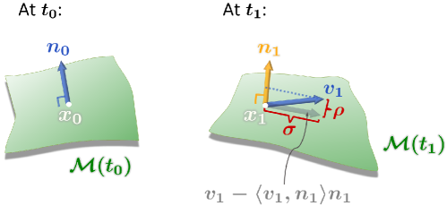
Figure 2: Definitions of normal repulsion $\rho$, cf. (3), and the tangential shear $\sigma$, cf. (4).

Specifically, at an arbitrary point $x_{0}$ in $\text{$\mathcal{M}$}(t_{0})$, we consider a unit surface normal $n_{0}(x_{0})$: Mapping $n_{0}(x_{0})$ under the linearized flow $DF_{t_{0}}^{t_{1}}(x_{0})$ from $t_{0}$ to $t_{1}$ yields a vector $v_{1}(x_{1})=DF_{t_{0}}^{t_{1}}(x_{0})n_{0}(x_{0})$, where $x_{1}=F_{t_{0}}^{t_{1}}(x_{0})$ is a point in $\text{$\mathcal{M}$}(t_{1})$. The vector $v_{1}(x_{1})$ will generally neither be of unit length nor perpendicular to the surface $\text{$\mathcal{M}$}(t_{1})$. Denoting the unit normal of $\text{$\mathcal{M}$}(t_{1})$ at $x_{1}$ by $n_{1}(x_{1})$, we introduce the normal repulsion $\rho$ as

$$\rho=||\left\langle v_{1},n_{1}\right\rangle n_{1}||=\left\langle v_{1},n_{1}\right\rangle,$$ (3)

where $\left\langle.,.\right\rangle$ is the Euclidean scalar product, and $||.||$ is the Euclidean norm. A large value of $\rho$ means that the component of $v_{1}(x_{1})$ normal to the surface $\text{$\mathcal{M}$}(t_{1})$ is large and, thus, material elements that were initially aligned with $n_{0}(x_{0})$ appear repelled from $\text{$\mathcal{M}$}(t_{1})$. Similarly, if the normal component of $v_{1}(x_{1})$ is small, then the components of $v_{1}(x_{1})$ tangent to $\text{$\mathcal{M}$}(t_{1})$ must be large, corresponding to attraction of material elements aligned with $n_{0}(x_{0})$ to the surface $\text{$\mathcal{M}$}(t_{1})$. Formally, we consider the normal repulsion as a function of the initial position $x_{0}$ and the surface normal $n_{0}(x_{0})$, i.e., $\rho=\rho(x_{0},n_{0})$. With this convention, $\text{$\mathcal{M}$}(t_{0})$ determines $\rho$. We now use $\rho$ to define hyperbolic LCSs as most repelling or attracting material surfaces:

Definition 2 (Repelling and attracting hyperbolic LCS (Blazevski2014, )).

A smooth material surface $\mathcal{M}(t)$ is a repelling (or attracting) hyperbolic LCS if the unit normals $n_{0}(.)$ of $\mathcal{M}(t_{0})$ maximize (or minimize) the normal repulsion function $\rho$ among all perturbations $n_{0}(.)\mapsto\tilde{n}_{0}(.)$, with $\tilde{n}_{0}:\mathcal{M}(t_{0})\rightarrow S^{2}$ denoting an arbitrary unit vector field.

We additionally require $\rho>1$ ($\rho<1$) for repelling (attracting) hyperbolic LCSs, which is automatically satisfied for incompressible flows.

Motivated by KAM tori and coherent vortex rings in fluid flows, we require elliptic LCSs to be tubular surfaces in the phase space. By a tubular surface, we mean a smooth surface that is diffeomorphic to a torus, cylinder, sphere or paraboloid. In order to capture the most influential tubular surfaces, Fig. 2 suggests considering elliptic LCSs as surfaces maximizing the tangential shear $\sigma$ under perturbations to the surface normal (Blazevski2014, ). This Lagrangian shear $\sigma$ is defined as

$$\sigma=||v_{1}-\left\langle v_{1},n_{1}\right\rangle n_{1}||=||v_{1}-\rho\,n_{1}||$$ (4)

(cf. Fig. 2). We consider the tangential shear $\sigma$ as a function of the initial position $x_{0}$ and the surface normal $n_{0}(x_{0})$, i.e., we write $\sigma=\sigma(x_{0},n_{0})$.

Definition 3 (Shear-maximizing elliptic LCS (Blazevski2014, )).

A tubular material surface $\mathcal{M}(t)$ is an elliptic LCS if the unit normals $n_{0}(.)$ of $\mathcal{M}(t_{0})$ maximize the tangential shear function $\sigma$ among all perturbations $n_{0}(.)\mapsto\tilde{n}_{0}(.)$, with $\tilde{n}_{0}:\mathcal{M}(t_{0})\rightarrow S^{2}$ denoting an arbitrary unit vector field.

As pointed out in (Oettinger2016, ), due to ever-present numerical inaccuracies, it is difficult to construct entire tubular surfaces that satisfy the strict requirement of pointwise maximal shear. A less restrictive definition of elliptic LCSs has been obtained recently by considering material surfaces $\mathcal{M}(t)$ that stretch nearly uniformly under the flow (Oettinger2016, ). Considering any point $x_{0}$ in $\text{$\mathcal{M}$}(t_{0})$, the linearized flow $DF_{t_{0}}^{t_{1}}$ maps any vector $e_{0}(x_{0})$ from the tangent space $\text{$T_{x_{0}}\mathcal{M}$}(t_{0})$ to a vector $e_{1}(x_{1})$ in $T_{x_{1}}\text{$\mathcal{M}$}(t_{1})$, where $x_{1}=F_{t_{0}}^{t_{1}}(x_{0})$. We define $\mathcal{M}(t)$ as nearly uniformly stretching at $x_{0}$ if all tangent vectors $e_{0}(x_{0})$ satisfy

$$||e_{1}(x_{1})||=\lambda(x_{0})\cdot||e_{0}(x_{0})||\text{\quad with\quad\ }\lambda(x_{0})\in[\sigma_{2}(x_{0})\cdot(1-\Delta),\sigma_{2}(x_{0})\cdot(1+\Delta)],$$ (5)

where $\sigma_{2}(x_{0})$ is the intermediate singular value of $DF_{t_{0}}^{t_{1}}(x_{0})$ (introduced below, cf. (6)); and $\Delta$ is a small stretching deviation ($0\leq\Delta\ll 1$). As shown in (Oettinger2016, ), setting $\lambda(x_{0})=\sigma_{2}(x_{0})$ (i.e., $\Delta=0$) is the only way to obtain a material surface that is exactly uniformly stretching at $x_{0}$ (cf. Fig. 3).

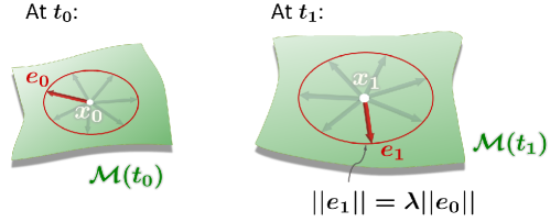
Figure 3: Local deformation of a pointwise uniformly stretching surface (cf. (5)): All tangent vectors based at $x_{0}$ stretch exactly by the same factor of $\lambda(x_{0})$ between times $t_{0}$ and $t_{1}$.

Definition 4 (Near-uniformly stretching elliptic LCS (Oettinger2016, )).

A tubular material surface $\mathcal{M}(t)$ is an elliptic LCS if it is nearly uniformly stretching at any point in $\text{$\mathcal{M}$}(t_{0})$.

Remark 1.

In (Oettinger2016, ), the stretching deviation $\Delta$ is chosen to be constant on $\text{$\mathcal{M}$}(t_{0})$. We could, however, let $\Delta$ vary on $\text{$\mathcal{M}$}(t_{0})$ and still obtain valid elliptic LCSs (as long as $0\leq\Delta\ll 1$). Requiring exact uniform stretching ($\Delta=0$) would be similarly restrictive as requiring maximal tangential shear (cf. Definition 3).

Remark 2.

Since $\sigma_{2}(x_{0})$ is given by the problem and generally not a constant function, the factor $\lambda=\lambda(x_{0})$ varies within the surface $\text{$\mathcal{M}$}(t_{0})$ even when $\Delta=0$. In two dimensions, however, it is possible to construct elliptic LCSs that stretch by a factor $\lambda$ that is constant on $\text{$\mathcal{M}$}(t_{0})$ (Haller2013, ).

Remark 3.

Other types of distinguished material surfaces revealing elliptic LCSs are level sets of the polar rotation angle (farazmand2015polar, ) and level sets of the Lagrangian-averaged vorticity (haller2015defining, ). These approaches are based on the notion of rotational coherence rather than stretching, and are hence not directly related to the variational approaches we review here.

From the linearization of the flow map $F_{t_{0}}^{t_{1}}$, we can derive explicit geometric conditions for both hyperbolic and elliptic LCSs (Definitions 2–4). These conditions are expressible in terms of eigenvectors and eigenvalues of the left and right Cauchy-Green strain tensors (cf. Remark 4 below). A fully equivalent, yet simpler picture is provided by the singular-value decomposition (SVD) of the the linearized flow map $DF_{t_{0}}^{t_{1}}(x_{0})$: The linearized flow map $DF_{t_{0}}^{t_{1}}(x_{0})$ (also called deformation gradient) maps vectors from the tangent space at $x_{0}$ onto their time-$t_{1}$ images in the tangent space at the point $x_{1}=F_{t_{0}}^{t_{1}}(x_{0})$. (Since the flow domain $U$ is in the Euclidean space $\mathbb{R}^{3}$, each of these tangent spaces is simply $\mathbb{R}^{3}$ as well.) In particular, $DF_{t_{0}}^{t_{1}}(x_{0})$ maps its three right-singular vectors $\xi_{1,2,3}(x_{0})$ onto its three left-singular vectors $\eta_{1,2,3}(x_{1})$, i.e.,

$$DF_{t_{0}}^{t_{1}}(x_{0})\xi_{i}(x_{0})=\sigma_{i}(x_{0})\cdot\eta_{i}(x_{1}),\qquad i=1,2,3,$$ (6)

see Fig. 4 and (TrefethenBauSpecific, ).

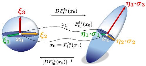
Figure 4: The deformation gradient $DF_{t_{0}}^{t_{1}}$ mapping its right-singular vectors $\xi_{1,2,3}$ onto its left-singular vectors $\eta_{1,2,3}$.

The singular vectors $\xi_{1,2,3}(x_{0})$ and the $\eta_{1,2,3}(x_{1})$ are unit vectors. Both the $\xi_{1,2,3}(x_{0})$ and the $\eta_{1,2,3}(x_{1})$ define an orthonormal basis of $\mathbb{R}^{3}$. The stretch factors $\sigma_{1,2,3}(x_{0})$ in (6) are the singular values of $DF_{t_{0}}^{t_{1}}(x_{0})$, which we assume to be distinct and ordered so that

$$0<\sigma_{1}(x_{0})<\sigma_{2}(x_{0})<\sigma_{3}(x_{0}).$$ (7)

The available LCS definitions (Blazevski2014, ; Oettinger2016, ) do not consider points where two singular values are equal.

We illustrate the kinematic role of the right-singular vectors $\xi_{1,2,3}(x_{0})$ by considering the stretch factor of a vector $v(x_{0})$, defined as

$$\Lambda_{t_{0}}^{t_{1}}(x_{0},v(x_{0}))=\frac{\left\|DF_{t_{0}}^{t_{1}}(x_{0})\,v(x_{0})\right\|}{||v(x_{0})||}.$$ (8)

Since $\sigma_{1}(x_{0})<\sigma_{2}(x_{0})<\sigma_{3}(x_{0})$, any vector $v(x_{0})$ parallel to $\xi_{3}(x_{0})$ maximizes the stretch factor $\Lambda_{t_{0}}^{t_{1}}(x_{0},.)$ among all vectors from $\mathbb{R}^{3}$. The direction $\xi_{1}(x_{0})$, on the other hand, minimizes $\Lambda_{t_{0}}^{t_{1}}(x_{0},.)$. We thus refer to the (right-) singular vector $\xi_{2}(x_{0})$ as the intermediate (right-) singular vector of $DF_{t_{0}}^{t_{1}}(x_{0})$. In many applications, the flow $F_{t_{0}}^{t_{1}}$ is volume-preserving (incompressible). Incompressibility means that $\sigma_{1}\sigma_{2}\sigma_{3}=1$ holds everywhere. Together with $0<\sigma_{1}<\sigma_{2}<\sigma_{3}$, this implies that $\sigma_{2}$ is the singular value closest to unity (cf. Appendix A). Accordingly, $\xi_{2}$ is the singular vector closest to unit stretching (i.e., $\Lambda_{t_{0}}^{t_{1}}=1$).

The backward-time flow map $F_{t_{1}}^{t_{0}}$ yields a similar interpretation for the left-singular vectors $\eta_{1,2,3}(x_{1})$: The backward-time deformation gradient, $DF_{t_{1}}^{t_{0}}(x_{1})$, satisfies $DF_{t_{1}}^{t_{0}}(x_{1})=\left[DF_{t_{0}}^{t_{1}}(x_{0})\right]^{-1}$. The right-singular vectors of $DF_{t_{1}}^{t_{0}}(x_{1})$ are, therefore, precisely the vectors $\eta_{1,2,3}(x_{1})$; the left-singular vectors of $DF_{t_{1}}^{t_{0}}(x_{1})$ are the $\xi_{1,2,3}(x_{0})$. In backward time, the $\eta_{1,2,3}(x_{1})$ hence play a similar role to $\xi_{1,2,3}(x_{0})$ in forward time. With the singular values of $DF_{t_{1}}^{t_{0}}(x_{1})$ being $[\sigma_{1,2,3}(x_{0})]^{-1}$, it is, however, the vector $\eta_{1}(x_{1})$ that maximizes $\Lambda_{t_{1}}^{t_{0}}.$ This means, the direction of largest stretching in backward time is $\eta_{1}(x_{1})$. Similarly, the vector $\eta_{3}(x_{1})$ coincides with the direction of least stretching in backward time; and $\eta_{2}(x_{1})$ is the intermediate (right-) singular vector of $DF_{t_{1}}^{t_{0}}(x_{1})$.

Remark 4.

By introducing the right Cauchy-Green strain tensor

$$C_{t_{0}}^{t_{1}}(x_{0})=\left[DF_{t_{0}}^{t_{1}}(x_{0})\right]^{T}DF_{t_{0}}^{t_{1}}(x_{0})\,,$$ (9)

where the $T$-superscript indicates transposition, we recover the singular vectors $\xi_{1,2,3}(x_{0})$ as eigenvectors of $C_{t_{0}}^{t_{1}}(x_{0})$. The associated eigenvalues of $C_{t_{0}}^{t_{1}}(x_{0})$ are $\lambda_{1,2,3}(x_{0})=[\sigma_{1,2,3}(x_{0})]^{2}.$ Similarly, introducing the left Cauchy-Green strain tensor (marsdenhughes1994specific, ) as

$$B_{t_{0}}^{t_{1}}(x_{1})=DF_{t_{0}}^{t_{1}}(x_{0})\left[DF_{t_{0}}^{t_{1}}(x_{0})\right]^{T},$$ (10)

where $x_{0}=F_{t_{1}}^{t_{0}}(x_{1})$, the left-singular vectors $\eta_{1,2,3}(x_{1})$ are the eigenvectors of $B_{t_{0}}^{t_{1}}(x_{1})$. The use of $C_{t_{0}}^{t_{1}}$ and $B_{t_{0}}^{t_{1}}$ is a common approach in the LCS literature (Haller2015, ; HallerSapsis2011, ). As it is, however, numerically advantageous to use SVD instead of eigendecomposition (Watkins2005NoEIGButSVD, ; karrasch2015attracting, ), we will not use the Cauchy-Green strain tensors here.

From the above it follows that the hyperbolic LCSs introduced in Definition 2 can be specified in terms of the vectors $\xi_{1}(x_{0})$, $\xi_{3}(x_{0})$ (or $\text{$\eta$}_{1}(x_{1})$, $\text{$\eta$}_{3}(x_{1})$). (For a proof, see (Blazevski2014, ), Appendix C.)

Proposition 1.

A smooth material surface is a repelling hyperbolic LCS if its time-$t_{0}$ position is everywhere normal to the direction $\xi_{3}$ of largest stretching in forward time; or, if its time-$t_{1}$ position is everywhere normal to the direction $\eta_{3}$ of least stretching in backward time.

Proposition 2.

A smooth material surface is an attracting hyperbolic LCS if its time-$t_{0}$ position is everywhere normal to the direction $\xi_{1}$ of least stretching in forward time; or, if its time-$t_{1}$ position is everywhere normal to the direction $\eta_{1}$ of largest stretching in backward time.

Elliptic LCSs (cf. Definitions 3, 4) can be constructed similarly in terms of the $\xi_{1,2,3}(x_{0})$ (or $\text{$\eta$}_{1,2,3}(x_{1}))$ and the $\sigma_{1,2,3}(x_{0})$:

Proposition 3.

A smooth material surface is pointwise shear-maximizing if its time-$t_{0}$ position is everywhere normal to one of the two directions

$$\tilde{n}{}^{\pm}=\tilde{\alpha}(\sigma_{1},\sigma_{2},\sigma_{3})\,\xi_{1}\pm\tilde{\gamma}(\sigma_{1},\sigma_{2},\sigma_{3})\,\xi_{3}.$$ (11)

Here $\tilde{\alpha},\,\tilde{\gamma}$ are positive functions of the singular values $\sigma_{1,2,3}$. (See (Blazevski2014, ) for the specific expressions for $\tilde{\alpha}$ and $\tilde{\gamma}$.)

Proof.

See (Blazevski2014, ), Theorem 1. ∎

Proposition 4.

A smooth material surface is nearly uniformly stretching if its time-$t_{0}$ position is everywhere normal to one of the two directions

$$n_{\lambda}^{\pm}=\alpha(\sigma_{1},\sigma_{2},\sigma_{3},\lambda)\,\xi_{1}\pm\gamma(\sigma_{1},\sigma_{2},\sigma_{3},\lambda)\,\xi_{3}.$$ (12)

Here $\alpha,\,\gamma$ are positive functions of the singular values $\sigma_{1,2,3}$, and $\lambda\in[\sigma_{2}(1-\Delta),\sigma_{2}(1+\Delta)]$ with $0\leq\Delta\ll 1$. (See (Oettinger2016, ) for the specific expressions for $\alpha$ and $\gamma$.)

Proof.

See (Oettinger2016, ), Proposition 1. ∎

IV Main result: An autonomous dynamical system for all Lagrangian coherent structures in 3D

As reviewed in Sec. III, all known LCSs in three dimensions are geometrically constrained by the singular vectors of the deformation gradient: Repelling hyperbolic LCSs are normal to the largest singular vector $\xi_{3}$ (Proposition 1); attracting hyperbolic LCSs normal to the smallest singular vector $\xi_{1}$ (Proposition 2); elliptic LCSs can be obtained as surfaces normal to certain linear combinations of $\xi_{1}$ and $\xi_{3}$ (Propositions 3, 4). All these definitions, therefore, pick out material surfaces $\mathcal{M}(t)$ which, at the initial time $t_{0}$, are perpendicular to a normal field $n$ of the general form

$$n=a\xi_{1}+c\xi_{3},$$ (13)

with real functions $a$ and $c$. In other words, any initial LCS surface $\mathcal{M}(t_{0})$ is normal to a linear combination of the smallest and largest singular vector of $DF_{t_{0}}^{t_{1}}$. Consequently, the intermediate singular vector $\xi_{2}$ must always lie in the surface $\mathcal{M}(t_{0})$. This means, $\mathcal{M}(t_{0})$ is necessarily tangent to the $\xi_{2}$-direction field. An integral curve of the $\xi_{2}$-direction field launched from an arbitrary point of the surface $\mathcal{M}(t_{0})$ will, therefore, remain confined to $\mathcal{M}(t_{0})$ upon further integration. In the language of dynamical systems theory, we summarize this observation as follows (cf. Fig. 5):

Theorem 1.

The initial position $\mathcal{M}(t_{0})$ of any hyperbolic LCS (Definition 2) or any elliptic LCS (Definitions 3, 4) is an invariant manifold of the autonomous dynamical system

$$x_{0}^{\prime}=\xi_{2}(x_{0}).$$ (14)

Similarly, final positions $\mathcal{M}(t_{1})$ of hyperbolic and elliptic LCSs are invariant manifolds of the autonomous dynamical system

$$x_{1}^{\prime}=\eta_{2}(x_{1}).$$ (15)

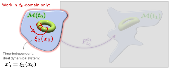
Figure 5: Schematic of an elliptic LCS $\text{$\mathcal{M}$}(t)$, revealed as a toroidal invariant manifold $\text{$\mathcal{M}$}(t_{0})$ of the autonomous dual dynamical system (14), cf. Theorem 1.

We refer to the autonomous systems (14)–(15) as the dual dynamical systems associated with the original, non-autonomous system (1) over the time interval $[t_{0},t_{1}]$. The dynamics of these dual systems are not equivalent to the non-autonomous dynamical system (1). Rather, the dual systems allow locating the LCSs associated with (1) using classical methods for autonomous dynamical systems (e.g., Poincaré maps).

Since we usually identify LCS surfaces at the initial time $t_{0}$ (cf. Sec. II), we will mostly discuss the $\xi_{2}$-system (14). Analogous results hold for the $\eta_{2}$-system (15).

Remark 5.

We refer to the right-hand side of (14) as the $\xi_{2}$-field, to its integral curves as $\xi_{2}$-lines, and to its invariant manifolds as $\xi_{2}$-invariant manifolds. Calling (14) a dual dynamical system guides our intuition, but requires some clarification: For (14) to be well-defined, we need to locally assign an orientation to the $\xi_{2}$-direction field. Along integral curves, once we assign an initial orientation, this can always be done in a smooth fashion (cf. Appendix C). With this prescription, the orientation of trajectories in the $\xi_{2}$-system is defined unambiguously. (Since the $\xi_{2}$-vectors in (14) are unit vectors, here, the evolutionary variable is arclength.)

Theorem 1 enables locating unknown LCSs of all types using only one equation: Any two-dimensional invariant manifold $\mathcal{S}(t_{0})$ of the $\xi_{2}$-system (14) is a surface that fulfills a necessary condition (i.e., tangency to $\xi_{2}$) required for the initial positions $\mathcal{M}(t_{0})$ of both hyperbolic and elliptic LCSs. Since invariant manifolds of (14) are already exceptional objects by themselves, any $\xi_{2}$-invariant manifold $\mathcal{S}(t_{0})$ that we obtain for a given dynamical system (1) is a relevant candidate for an LCS surface $\mathcal{M}(t_{0})$.

Since the LCS normals from Propositions 1–4 do not encompass all linear combinations of $\xi_{1}$ and $\xi_{3}$, the converse of Theorem 1 does not hold. In other words, a $\xi_{2}$-invariant manifold $\mathcal{S}(t_{0})$ does not necessarily correspond to an LCS $\mathcal{M}(t_{0})$. To fully determine whether $\mathcal{S}(t_{0})$ does satisfy one of the Definitions 2–4, therefore, one has to verify tangency to a second vector field (cf. Appendix D). In applications, however, it is enough to categorize an LCS candidate qualitatively as either elliptic, hyperbolic repelling or attracting. As seen in the examples below (cf. Sec. V), we can then omit the procedure in Appendix D and examine both the topology of an LCS candidate $\mathcal{S}(t_{0})$ and its image under the flow map, $\mathcal{S}(t_{1})$, to assess if the material surface $\mathcal{S}(t)$ belongs to any of the three general LCS types: Any tubular surface $\mathcal{S}(t_{0})$ is a candidate for an elliptic LCS, any sheet-like surface $\mathcal{S}(t_{0})$ is a candidate for a hyperbolic LCSs. Mapping $\mathcal{S}(t_{0})$ under the flow map reveals if $\mathcal{S}(t)$ indeed holds up as an elliptic or hyperbolic LCS.

As outlined in Sec. I, previous approaches (Blazevski2014, ; Oettinger2016, ) locate LCSs of all the types in three dimensions (Definitions 2–4) using the expressions for their surface normals from Propositions 1–4. Specifically, these methods sample the flow domain using extended families of two-dimensional reference planes. Taking the cross product between the LCS normal and the normal of each reference plane then defines two-dimensional direction fields to which the unknown LCS surfaces need to be tangent. These two-dimensional fields depend on the type of LCS; in particular, for the near-uniformly stretching LCSs, by (12), there are two parametric families of normal fields $n_{\lambda}^{\pm}$, which need to be sampled using a dense set of $\lambda$-parameters. Overall, therefore, one has to perform integrations of a large number of two-dimensional direction fields. (E.g., (Oettinger2016, ) obtained elliptic LCSs in the steady Arnold-Beltrami-Childress from integral curves of 1600 distinct direction fields.) Accordingly, this procedure typically produces a large collection of possible intersection curves between reference planes and LCSs. As a second step, these approaches require identification of curves from this collection that can be interpolated into LCS surfaces. Despite these efforts, the previous approaches (Blazevski2014, ; Oettinger2016, ) do not enforce Theorem 1 and hence cannot guarantee more accurate LCS results than the present approach. An advantage is, however, that these approaches (Blazevski2014, ; Oettinger2016, ) inherently distinguish between the specific normal fields given in Propositions 1–4 and hence do not require further analysis to determine the LCS type.

Clearly, opposed to the previous methods (Blazevski2014, ; Oettinger2016, ) described above, analyzing the $\xi_{2}$-system (14) is a conceptually simpler approach to obtaining LCSs in three dimensions: First, the $\xi_{2}$-field is a single direction field suitable for all types of LCSs. Secondly, as opposed to considering a large number of independent two-dimensional equations, the $\xi_{2}$-system (14) is defined on a three-dimensional domain. In comparison to the methods in (Blazevski2014, ; Oettinger2016, ), this eliminates the effort of handling large amounts of unutilized data and eliminates possible issues with the placement of reference planes. A full determination of the LCS types, however, requires verifying tangency to a second vector field (cf. Appendix D).

In two dimensions, initial positions of LCSs can be viewed as invariant manifolds of differential equations similar to (14). There, however, the available LCS types (hyperbolic, parabolic and elliptic LCSs (Haller2011a, ; Farazmand2014a, ; Haller2013, )) do not satisfy a single common differential equation: With only two right-singular vectors $\tilde{\xi}{}_{1,2}$ in two dimensions (and no counterpart to the intermediate eigenvector $\xi_{2}$ in three dimensions), the initial positions of hyperbolic and parabolic LCSs are defined by integral curves of either $\tilde{\xi}_{1}$ or $\tilde{\xi}_{2}$ (Haller2011a, ; Farazmand2014a, ). Similarly, elliptic LCSs are limit cycles of direction fields belonging to a parametric family of linear combinations of $\tilde{\xi}_{1}$ and $\tilde{\xi}_{2}$ (Haller2013, ). Therefore, there cannot be a counterpart to Theorem 1 in two dimensions. Locating the LCSs in two dimensions requires analyzing all these differential equations separately.

In four dimensions and higher, there are no suitable extensions to the LCS definitions from Sec. III, and hence there is no counterpart to Theorem 1 either (cf. Appendix B).

V Examples

In this section, we consider several (steady and time-aperiodic) flows and locate their LCSs by finding invariant manifolds of their associated $\xi_{2}$-fields. Our approach is to run long $\xi_{2}$-trajectories which may asymptotically accumulate on normally attracting invariant manifolds of the $\xi_{2}$-field (for numerical details, see Appendix C). By Theorem 1, such invariant manifolds are candidates for time $t_{0}$-positions of LCSs. Obtaining the LCSs as attractors in the $\xi_{2}$-system ensures their robustness, whereas this property does not generally hold for them in the original non-autonomous system. (For incompressible flows, such as the examples in this section, there are no attractors at all.)

For a generally applicable numerical algorithm, a more refined method for obtaining two-dimensional invariant manifolds in three-dimensional, autonomous dynamical systems needs to be combined with the ideas presented here (cf. Sec. VI). We postpone these additional steps to future work.

We first consider steady examples where transport barriers are known from other approaches, and hence the results obtained from the $\xi_{2}$-system are readily verified. We then move on to an example with a temporally aperiodic velocity field.

V.1 Cat’s eye flow

In Cartesian coordinates $(x,y,z)$, consider a vector field

$$u(x,y,z)=\left(\begin{array}[]{c}-\partial_{y}\psi(x,y)\\ \partial_{x}\psi(x,y)\\ W\circ\psi(x,y)\end{array}\right),$$ (16)

where $W$, $\psi$ are smooth, real-valued functions, and $\psi$ is a stream function, i.e., $\Delta\psi=F(\psi)$ for some smooth function $F$. Any velocity field $u$ satisfying (16) is a solution of the Euler equations of fluid motion in three dimensions (majda2002xi2dual, ). We consider the two-and-a-half-dimensional Cat’s eye flow (majda2002xi2dual, ), given by (16) with $W(\psi)=\exp(\psi)$ and

$$\psi(x,y)=-\log[c\,\cosh(y)+\sqrt{c^{2}-1}\cos(x)],\quad c=2.$$ (17)

We assume that $u=u(x,y,z)$ is defined on the cylinder $S^{1}\times\mathbb{R}^{2}$, with $x\in\left[0,2\text{$\pi$}\right)$. Because $u$ only depends on the $x,y$-coordinates here, i.e., $u=u(x,y)$, any flow generated by a velocity field $u$ as in (16) is called two-and-a-half-dimensional.

Denoting the trajectory passing through $(x_{0},y_{0},z_{0})$ at time $t_{0}$ by $(x(t),y(t),z(t))$, the flow map takes the form $F_{t_{0}}^{t_{1}}(x_{0},y_{0},z_{0})=(x_{0},y_{0},z_{0})^{T}+\int_{t_{0}}^{t_{1}}u(x(s),y(s))ds$. Thus, the flow map $F_{t_{0}}^{t_{1}}$ is linear in $z_{0}$. Consequently, the deformation gradient $DF_{t_{0}}^{t_{1}}$, its singular values $\sigma_{1,2,3}$, and singular vectors $\xi_{1,2,3}$ do not depend on $z_{0}$.

Identifying the coordinates of the domain $D$ of initial positions $(x_{0},y_{0},z_{0})$ with $(x,y,z)$, we we cannot expect, however, that any of the $\xi_{1,2,3}$-fields will have a vanishing $z$-component, i.e., be effectively two-dimensional.

For the numerical integrations of the $\xi_{2}$-field (14), we choose 20 representative initial conditions $p_{0}$ in the plane $z=0$ and, imposing the initial orientation such that the $z$-component of $\xi_{2}(p_{0})$ is positive, we compute $\xi_{2}$-lines up to arclength $s=500$. As the time-interval, we consider $[t_{0},t_{1}]=[0,100]$. We show the results in Fig. 6, together with level sets of $\psi$ that correspond to the values $\psi(p_{0})$.

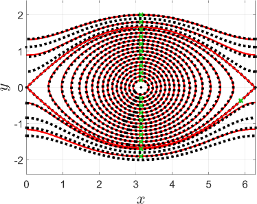
Figure 6: Cat’s eye flow: Comparison between $x,y$-projections of $\xi_{2}$-lines, displayed for arclength $s\in[0,500]$, (solid red curves) and level sets of the stream function $\psi$ (dotted black curves). The $\xi_{2}$-lines have nonzero $z$-components and are confined to generalized cylinders. The initial conditions of the $\xi_{2}$-lines, $p_{0}$, are marked by green crosses.

Each level set of $\psi$ defines a two-dimensional invariant manifold of the Cat’s eye flow. The $\xi_{2}$-lines are well-aligned with the corresponding level sets of $\psi$, including the separatrix, showing consistency between the possible locations of LCSs and the invariant manifolds of the Cat’s eye velocity field. (We note that full alignment would require sampling the infinite-time dynamics of the Cat’s eye flow, i.e., letting $t_{1}\rightarrow\infty$ (Haller2015, ).) We observe that the $x,y$-projection of each $\xi_{2}$-line is a periodic orbit, and thus, each $\xi_{2}$-line is confined to a generalized (two-dimensional) cylinder.

V.2 Steady ABC flow

Our second steady example is a fully three-dimensional solution of the Euler equations, the steady Arnold-Beltrami-Childress (ABC) flow

$$u(x,y,z)=\left(\begin{array}[]{c}A\sin(z)+C\cos(y)\\ B\sin(x)+A\cos(z)\\ C\sin(y)+B\cos(x)\end{array}\right),$$ (18)

with $A=\sqrt{3},\,B=\sqrt{2},\,C=1$. The coordinates in (18) are Cartesian, with $(x,y,z)\in[0,2\pi]^{3}$ and periodic boundary conditions imposed in $x$, $y$ and $z$.

Using the plane $z=0$ as a Poincaré section, and placing in it a square grid of $20\times 20$ initial positions (cf. Fig. 7a), we integrate trajectories of (18) from time 0 to time $2\cdot 10^{4}$. Retaining only their long-time behavior from the time interval $[10^{4},2\cdot 10^{4}]$, we obtain a large number of iterations of the Poincaré map (cf. Fig. 7b). The plot reveals 5 vortical regions surrounded by a chaotic sea. Each of the vortical regions contains a family of invariant tori that act as transport barriers.

Here we want to obtain both elliptic and hyperbolic LCSs using the dual $\xi_{2}$-system (14) for $[t_{0},t_{1}]=[0,10]$. The phase space of the $\xi_{2}$-system coincides with the domain of (18). In contrast to trajectories of $u$, independently of the time interval $[t_{0},t_{1}]$, we can run $\xi_{2}$-lines as long as we need. Choosing the same Poincaré section and the same grid of initial conditions as above (cf. Fig. 7a), we integrate $\xi_{2}$-lines (initially aligned with $(0,0,1)$) up to arclength $5\cdot 10^{4}$. Retaining segments from the arclength interval $[4\cdot 10^{4},5\cdot 10^{4}]$, and intersecting these segments with the $z=0$ plane, we obtain iterations of a dual Poincaré map (cf. Fig. 7c).

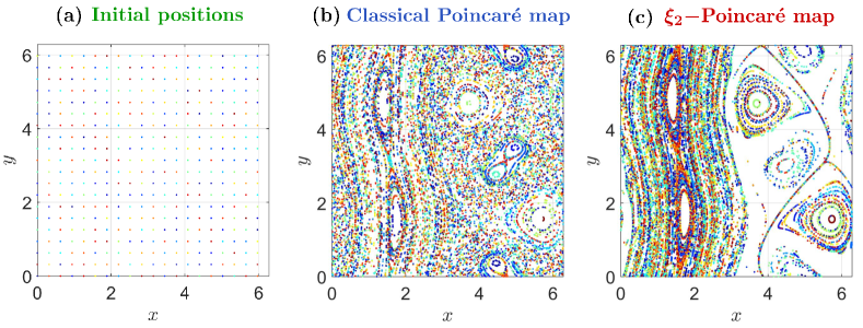
(a)

(b)

(c)

Figure 7: Steady ABC flow: Comparison of Poincaré maps at $z=0$. (a) Grid of 20$\times$20 initial positions in the $z=0$-plane. (b) Poincaré map of (18) obtained from trajectories over $[10^{4},2\cdot 10^{4}]$, indicating invariant manifolds of the ABC flow; (c) Poincaré map of the $\xi_{2}$-field, obtained from $\xi_{2}$-lines over the arclength interval $[4\cdot 10^{4},5\cdot 10^{4}]$, indicating initial positions of LCSs.

This Poincaré map indicates invariant manifolds of the dual $\xi_{2}$-system. Specifically, the principal vortices of the ABC flow correspond to families of invariant tori of the $\xi_{2}$-field (cf. Fig. 7c), which are candidates for initial positions of elliptic LCSs. The tori of the $\xi_{2}$-system are similar to the invariant tori obtained from the classical Poincaré map (cf. Fig. 7b). In the region corresponding to the chaotic sea, however, the $\xi_{2}$-field is strongly dissipative and thus reveals a candidate for a transport barrier in the ABC flow that has no counterpart in the classical Poincaré map obtained from the asymptotic dynamics of the incompressible system (18): We see a structure that has a large basin of attraction in the dual dynamics of the $\xi_{2}$-system and, secondly, spans the entire domain. In Sec. V.3, we will examine a slightly perturbed version of this structure in detail, finding that it is a hyperbolic repelling LCS.

We note that computing Poincaré maps for the $\xi_{2}$-system does not imply applying the flow map $F_{t_{0}}^{t_{1}}$ repetitively. Iterating a $\xi_{2}$-based Poincaré map simply serves to refine our understanding of the LCSs associated with $F_{t_{0}}^{t_{1}}$. Indeed, the iterated Poincaré map highlights intersections of fixed LCSs with a given plane of the $\xi_{2}$-system in more and more detail.

V.3 Time-aperiodic ABC-type flow

We next use the dual $\xi_{2}$-system (14) to analyze a time-aperiodic modification of the ABC flow, given by (18) with the replacements

$$B\mapsto\tilde{B}(t) = B+B\cdot k_{0}\tanh(k_{1}t)\cos[(k_{2}t)^{2}],$$ (19)

$$C\mapsto\tilde{C}(t) = C+C\cdot k_{0}\tanh(k_{1}t)\sin[(k_{3}t)^{2}].$$

Neither a classical Poincaré map nor any other method requiring long trajectories are options here, due to the temporal aperiodicity of the system. In (19), we choose $k_{0}=0.3$, $k_{1}=0.5$, $k_{2}=1.5$ and $k_{3}=1.8$. We show the functions $\tilde{B}(t)-B$, $\tilde{C}(t)-C$ in Fig. 8.

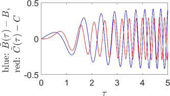
Figure 8: Time dependence of the coefficient functions $\tilde{B}(t)$, $\tilde{C}(t)$ in (19).

Elliptic LCSs in similar time-aperiodic ABC-type flows have been obtained in (Blazevski2014, ; Oettinger2016, ); hyperbolic repelling LCSs in (Blazevski2014, ), although only of small extent in the $z$-direction.

Considering the $\xi_{2}$-system for the time interval $[t_{0},t_{1}]=[0,5]$, we compute the dual Poincaré map (cf. Fig. 9a). The algorithm and numerical settings are the same as in Sec. V.2.

(a)

(b)

Figure 9: Time-aperiodic ABC-type flow: Arc segments of $\xi_{2}$-lines (corresponding to arclength $s\in[4\cdot 10^{4},5\cdot 10^{4}]$) reveal locations of elliptic and hyperbolic LCSs. (a) Dual Poincaré map, showing intersections between the Poincaré section $z=0$ and possible time-$t_{0}$ locations of elliptic and hyperbolic LCSs. (b) Possible time-$t_{0}$ locations of elliptic and hyperbolic LCSs: The structure in green (indicating a hyperbolic LCS) consists of segments from several $\xi_{2}$-lines. The tubular surfaces (indicating elliptic LCSs) are fitted from point data of individual $\xi_{2}$-lines. Here we use the periodicity of the phase space to extend the domain slightly beyond $[0,2\pi]^{3}$.

Compared to Fig. 7c, there are a few structures that persist under the time-aperiodic perturbation (19) to the velocity field (18): The large (presumably hyperbolic) structure spanning the flow domain is still present and barely changed. In Fig. 9b, we show $\xi_{2}$-lines corresponding to this hyperbolic LCS candidate (green). The $\xi_{2}$-lines indicate a complicated surface which they, however, do not cover densely. Regarding elliptic structures, instead of entire families of $\xi_{2}$-invariant tori, we are left with three large elliptic structures, each with a sizable domain of attraction (cf. Fig. 9a). The $\xi_{2}$-lines corresponding to these elliptic structures yield tori, which we show as tubular surfaces in Fig. 9b (red, blue, yellow). The dual Poincaré map (Fig. 9a) also shows that, inside two of these tori, there are additional, smaller elliptic structures. By plotting the $\xi_{2}$-lines corresponding to these smaller objects (not shown), we find that the surfaces they indicate are not tori and thus ignore them in our search for LCS candidates.

In Fig. 10a, we represent the yellow tubular surface from Fig. 9b in toroidal coordinates

$$\bar{x} = (x-x_{c}(z)+R_{1})\cos(z),$$ (20)

$$\bar{y} = (x-x_{c}(z)+R_{1})\sin(z),$$

$$\bar{z} = R_{2}(y-y_{c}(z)),$$

with $R_{1}=2,\,R_{2}=1$.

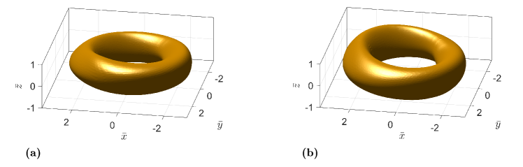
(a)

(b)

Figure 10: Time-aperiodic ABC-type flow: Mapping one of the tubular surfaces obtained from the $\xi_{2}$-lines (cf. Fig. 9b, yellow) under the flow map $F_{0}^{5}$, we confirm that this surface is a useful elliptic LCS. (a) Elliptic LCS surface at time $t_{0}=0$. (b) Elliptic LCS surface at time $t_{1}=5$.

In (20), the functions $x_{c}(z),\,y_{c}(z)$ are the $x,$ $y$ coordinates of the (approximate) vortex center. (For evaluating $x_{c}(z)$ and $y_{c}(z)$, we use our numerical values from previous work (Oettinger2016, ).) Mapping the resulting torus under the flow map $F_{0}^{5}$, we see that it does advect coherently over the interval $[t_{0},t_{1}]=[0,5]$ (cf. Fig. 10b). Therefore, even though this surface was just obtained from tangency to $\xi_{2}$ (a necessary condition for Definition 4), it renders a full-blown elliptic LCS.

We next examine locally whether the complicated green structure from Fig. 9b indeed corresponds to a hyperbolic LCS (Definition 2): In Fig. 11a, we take an illustrative part of the domain and interpolate a surface from the $\xi_{2}$-lines (green). Centered around a point in the surface, we additionally place a sphere of tracers (purple). Mapping the two objects forward in time under the flow map $F_{0}^{1}$, we see that the tracers deform into an ellipsoid that is most elongated in the direction normal to the advected surface (cf. Fig. 11b).

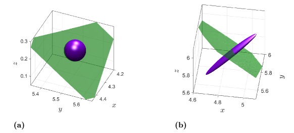
(a)

(b)

Figure 11: Time-aperiodic ABC-type flow: Local impact of the hyperbolic repelling LCS surface (interpolated from $\xi_{2}$-lines). (a) Zoom-in on the hyperbolic repelling LCS surface at time $t_{0}=0$ (green), shown together with a sphere formed by tracers (purple). (b) Time-1 positions of the hyperbolic repelling LCS surface and the deformed tracer sphere (obtained under $F_{0}^{1}$).

Considering Proposition 1 and Fig. 4, we thus classify this structure as a repelling hyperbolic LCS. (For an approach to confirming this globally, see Appendix D.) Considering Fig. 9b, we see that this structure is much larger than the hyperbolic LCS obtained for a similar time-aperiodic ABC-type flow in previous work (cf. (Blazevski2014, ), Fig. 15).

By Theorem 1, we can also take the direction field $\eta_{2}$ and repeat the above analysis. Using the same algorithm and numerical parameters as for the previous $\xi_{2}$-Poincaré map (cf. Fig. 9a), except that we now take the backward-time flow map $F_{5}^{0}$ instead of $F_{0}^{5}$, we obtain a Poincaré map for the dual dynamical system $x_{1}^{\prime}=\eta_{2}(x_{1})$ (cf. Fig. 12).

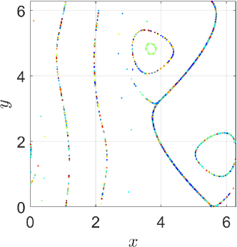
Figure 12: Dual Poincaré map obtained from $x_{1}^{\prime}=\eta_{2}(x_{1})$, showing intersections between the Poincaré section $z=0$ and possible time-$t_{1}$ locations of elliptic and hyperbolic LCSs.

This Poincaré map reveals possible time-$t_{1}$ positions of LCSs. The result is similar to the $\xi_{2}$-Poincaré map (cf. Fig. 9a), showing again a large hyperbolic structure, and the time-$t_{1}$ positions of the tori obtained earlier (cf. Fig. 9b).

We perform a local deformation analysis for the large hyperbolic structure indicated by Fig. 12: From a sample part of the $\eta_{2}$-lines corresponding to this structure, we fit a surface (cf. Fig. 13b, colored green) and map it backward in time under $F_{5}^{4}$, obtaining a surface at time $t=4$ (cf. Fig. 13a, green).

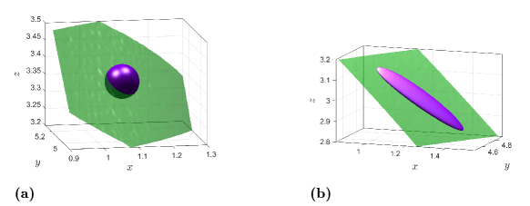
(a)

(b)

Figure 13: Time-aperiodic ABC-type flow: Local impact of the hyperbolic attracting LCS surface (fitted from $\eta_{2}$-lines). (a) Zoom-in on the hyperbolic attracting LCS surface at time $t=4$ (green), shown together with a sphere formed by tracers (purple). (b) Time-$t_{1}$ positions of the hyperbolic attracting LCS surface and the deformed tracer sphere (obtained under $F_{4}^{5}$).

Then we place a small tracer sphere (purple) in this part of the surface. Mapping both the time-4 surface and the tracer sphere forward in time under $F_{4}^{5}$, we find that the tracers fully align with the surface (cf. Fig. 13b). By Proposition 2 and Fig. 4, this suggests that the large hyperbolic structure from Fig. 12 belongs to the time-$t_{1}$ position of an attracting hyperbolic LCS. (For confirming this globally, see Appendix D.)

Remark 6.

With the present approach, for incompressible flows, it is generally easier to obtain attracting hyperbolic LCSs $\mathcal{M}(t_{1})$ at time $t_{1}$, rather than at time $t_{0}$: An attracting LCS at time $t_{0}$ is a surface $\mathcal{M}(t_{0})$ parallel to $\xi_{2}$ and $\xi_{3}$ (cf. Proposition 2). Mapping $\mathcal{M}(t_{0})$ to $\mathcal{M}(t_{1})$, the area element changes by a factor of $\sigma_{2}\sigma_{3}$. Due to incompressibility ($\sigma_{1}\sigma_{2}\sigma_{3}=1$), any attracting LCS is guaranteed to stretch in forward-time ($\sigma_{2}\sigma_{3}>1$). Since separation can, e.g., grow exponentially in time ($\sigma_{3}\propto\exp(t_{1}-t_{0})$), we generally expect the stretching of an attracting LCS to be substantial ($\sigma_{2}\sigma_{3}\gg 1$). At the final time $t_{1}$, we thus expect that any attracting LCS of global impact, $\mathcal{M}(t_{1})$, traverses a significant portion of the phase space. At time $t_{0}$, on the other hand, the surface $\mathcal{M}(t_{0})$ can still be very small. In this sense, seeking LCSs as invariant manifolds of the $\eta_{2}$-field is generally easier than using the $\xi_{2}$-field. For repelling LCSs, which shrink between times $t_{0}$ and $t_{1}$, the converse holds. (In two dimensions, the challenges of computing repelling and attracting hyperbolic LCSs at different times $t$* are similar (Farazmand2013, ; Karrasch201583, ).)

In summary, compared to previous methods of identifying LCSs from various two-dimensional direction fields (Blazevski2014, ; Oettinger2016, ), the advantage of the present approach is that it reveals both hyperbolic and elliptic LCSs from integrations of a single direction field. Instead of using multiple one-dimensional Poincaré sections (Blazevski2014, ; Oettinger2016, ), we can therefore search LCSs globally by using two-dimensional Poincaré sections (cf. Figs. 7c, 9a, 12). Finally, as opposed to classical Poincaré maps that require autonomous or time-periodic systems, the dual Poincaré map is well-defined for any non-autonomous system. We in fact treat autonomous, time-periodic and time-aperiodic dynamical systems on the same footing, while still benefiting from the advantages that a classical Poincaré map offers.

VI Conclusions

We have presented a unified approach to obtaining elliptic and hyperbolic LCSs in three-dimensional unsteady flows. In contrast to prior methods based on different direction fields for different types of LCSs (Blazevski2014, ; Oettinger2016, ), we obtain a common direction field, the intermediate eigenvector field, $\xi_{2}(x_{0})$, of the right Cauchy-Green strain tensor. Initial positions of all variational LCSs in three dimensions are necessarily invariant manifolds of this autonomous direction field. Equivalently, LCS final positions are invariant manifolds of the intermediate eigenvector field, $\eta_{2}(x_{1})$, of the left Cauchy-Green strain tensor. We can thus identify LCS surfaces globally by classic methods for autonomous dynamical systems. While the $\xi_{2}$- and $\eta_{2}$-systems by themselves do not discriminate between LCS types, the procedure from Appendix D outlines how to numerically assess the LCS type if needed.

Overall, the present approach is significantly simpler than previous numerical methods (Blazevski2014, ; Oettinger2016, ), and reveals larger hyperbolic LCSs in the time-aperiodic ABC-type flow than seen in a comparable example from previous work (Blazevski2014, ). An important advantage of our approach is that LCSs are attractors of the generally dissipative $\xi_{2}$-system, which is not the case in the original, typically incompressible system. Obtaining the LCSs as attractors of the dual $\xi_{2}$-system also guarantees their structural stability, implying that these structures will persist under small perturbations to the underlying flow. Our approach is restricted to three-dimensional systems, which is, however, highly relevant for fluid mechanical applications.

With the examples of Sec. V, we have illustrated the ability of the $\xi_{2}$-system to reveal LCSs. For a broadly applicable numerical method, further development is required. Computing two-dimensional invariant manifolds of the $\xi_{2}$-field by simply running long integral curves is not always efficient. General approaches for growing global stable and unstable manifolds of autonomous, three-dimensional vector fields are, however, available in the literature (cf. (krauskopf2005survey, ) for a review). We expect that a general computational method for obtaining LCSs from the $\xi_{2}$-system (14) can be most easily developed by transferring one of these available approaches to computing invariant manifolds from the setting of vector fields to direction fields. For a given dynamical system, one would first compute the $\xi_{2}$-field on a grid, and then apply the most suitable method for growing invariant manifolds to construct LCSs globally in the dual $\xi_{2}$-system.

Appendix A For incompressible flows, $\sigma_{2}$ is the singular value of $DF_{t_{0}}^{t_{1}}$ closest to unity

We clarify our statement that $0<\sigma_{1}<\sigma_{2}<\sigma_{3}$ and incompressibility (i.e., $\sigma_{1}\sigma_{2}\sigma_{3}=1$) imply that $\sigma_{2}$ is the singular value of $DF_{t_{0}}^{t_{1}}$ closest to unity. We first note that $\sigma_{1}=\sqrt[3]{\sigma_{1}^{3}}<\sqrt[3]{\sigma_{1}\sigma_{2}\sigma_{3}}=1$, and, similarly, $\sigma_{3}>1$. In general, it is unclear whether $\sigma_{2}<1$, $\sigma_{2}=1$, or $\sigma_{2}>1$. Due to the inequalities

$$\sigma_{1}<\min\left\{\sigma_{2},\frac{1}{\sigma_{2}}\right\}\leq 1\leq\max\left\{\sigma_{2},\frac{1}{\sigma_{2}}\right\}<\sigma_{3},$$ (21)

however, we consider $\sigma_{2}$ as the singular value closest to unity. Eq. 21 follows from a more general statement:

Lemma 1.

Given any three real numbers $a,$ $b,$ and c satisfying $0<a<b<c$, denoting their geometric mean by

$$m=\sqrt[3]{abc},$$ (22)

we have

$$\frac{a}{m}<\min\left\{\frac{b}{m},\frac{m}{b}\right\}\leq 1\leq\max\left\{\frac{b}{m},\frac{m}{b}\right\}<\frac{c}{m}.$$ (23)

Proof.

Denoting the natural logarithm by $\log$, we introduce $M=\log(m)$, $A=\log(a),$ $B=\log(b),$ and $C=\log(c)$. Taking the logarithm of (22), we then obtain

$$3M=A+B+C.$$ (24)

Furthermore, since $a=\sqrt[3]{a^{3}}<\sqrt[3]{abc}=m,$ we have

$$M-A>0,$$ (25)

and, similarly,

$$C-M>0.$$ (26)

1. For the first inequality in (23), we show that $a/m<m/b$. By strict monotonicity of the logarithm, this is equivalent to $\log\left(\tfrac{a}{m}\right)<\log\left(\tfrac{m}{b}\right),$ which we verify as follows:

   $$\log\left(\tfrac{a}{m}\right)=A-M\stackrel{{\scriptstyle\text{(\ref{eq:log_abc_inequalities})}}}{{=}}3M-B-C-M=(M-B)-(C-M)\stackrel{{\scriptstyle\text{(\ref{eq:CgtrM})}}}{{<}}M-B=\log\left(\tfrac{m}{b}\right).$$

   For the last inequality in (23), we can similarly show that $m/b<c/m$ (using (25) instead of (26)).

2. We show that $\min\left\{\log\left(\frac{b}{m}\right),\log\left(\frac{m}{b}\right)\right\}\leq 0$, which is equivalent to $\min\left\{\frac{b}{m},\frac{m}{b}\right\}\leq 1$. To verify the former inequality, we use that the minimum of any two real numbers $r_{1}$ and $r_{2}$ satisfies $\min\{r_{1},r_{2}\}=\tfrac{r_{1}+r_{2}}{2}-\tfrac{\left|r_{1}-r_{2}\right|}{2}.$ We obtain

   $$\min\left\{\log\left(\tfrac{b}{m}\right),\log\left(\tfrac{m}{b}\right)\right\}=\tfrac{1}{2}\left[(B-M)+(M-B)\right]-\tfrac{1}{2}\left|(B-M)-(M-B)\right|,$$

   and, thus,

   $$\min\left\{\log\left(\tfrac{b}{m}\right),\log\left(\tfrac{m}{b}\right)\right\}=-\left|B-M\right|\leq 0.$$

   Similarly, we can use $\max\{r_{1},r_{2}\}=\tfrac{r_{1}+r_{2}}{2}+\tfrac{\left|r_{1}-r_{2}\right|}{2}$ and show that $1\leq\max\left\{\frac{b}{m},\frac{m}{b}\right\}.$

∎

Setting $a=\sigma_{1}$, $b=\sigma_{2},$ $c=\sigma_{3}$ and $m=1$, Lemma 1 implies (21).

Appendix B Theorem 1 and higher dimensions

We discuss the possibility of a counterpart to our main result, Theorem 1, in higher dimensions. We start with four dimensions, where there are four singular vectors $\xi_{1,2,3,4}$. As in Sec. III, we label them such that the corresponding singular values $\sigma_{1,2,3,4}$ are in ascending order.

Example.

As a prerequisite, we would need to extend, e.g., the notion of a hyperbolic repelling LCS (cf. Definition 2) from three to four dimensions. As in Proposition 1, we would need a three-dimensional hypersurface $\mathcal{M}(t_{0})$ in $\mathbb{R}^{4}$ which is normal to $\xi_{4}$ and hence tangent to $\xi_{1,2,3}$ everywhere. It is not a priori obvious whether such a geometry is possible or not.

Consider a small open ball $B\subset\mathbb{R}^{4}$ where the singular values $\sigma_{1,2,3,4}$ are distinct. Within $B$, we may assume that the $\xi_{1,2,3,4}$-fields are smooth vector fields. We denote the Lie bracket between two such vector fields $v$ and $w$ by $[v,w]$.

We want to construct a three-dimensional hypersurface $\mathcal{M}(t_{0})$ such that $\mathcal{M}(t_{0})\cap B$ is normal to $\xi_{4}$. This is possible only if the fields $\xi_{1,2,3}$ satisfy

$$[\xi_{1},\xi_{2}],[\xi_{1},\xi_{3}],[\xi_{2},\xi_{3}]\in\text{span}\{\xi_{1},\xi_{2},\xi_{3}\}$$ (27)

for all points in $\mathcal{M}(t_{0})\cap B$ (cf., e.g., (Lee2012involutive, )). Conditions (27) are equivalent to the Frobenius conditions

$$\left\langle[\xi_{1},\xi_{2}],\xi_{4}\right\rangle=0,\,\left\langle[\xi_{1},\xi_{3}],\xi_{4}\right\rangle=0,\,\left\langle[\xi_{2},\xi_{3}],\xi_{4}\right\rangle=0.$$ (28)

(In the context of LCSs, such conditions have already been considered in (Blazevski2014, ).) Unless 0 is a critical value, by the Preimage Theorem (guillemin1974differential, ), each of the three conditions in (28) defines a codimension-one submanifold in $B$. Now there are two main possibilities:

Case 1: We suppose that 0 is a regular value for all conditions in (28). Since the conditions (28) are generally independent from each other, the subset $S$ of $B$ where all three conditions are satisfied simultaneously is codimension-three, i.e., a line. For $\mathcal{M}(t_{0})$ to be a well-defined repelling LCS, we need $\mathcal{M}(t_{0})\cap B$ to be a subset of $S.$ By our assumption, however, $\mathcal{M}(t_{0})\cap B$ is a three-dimensional hypersurface. Since $S$ is only one-dimensional, we have reached a contradiction.

Case 2: The remaining possibility is that 0 is a critical value for at least one of the conditions in (28). Then there is no general restriction on the geometry of the corresponding zero-level sets from (28). In particular, if 0 is critical value for at least two of the three conditions in (28), then the subset $S$ of $B$ where all three conditions are satisfied simultaneously can be a three- or four-dimensional manifold. In this case, $S$ can contain a three-dimensional surface $\mathcal{M}(t_{0})\cap B$ and, thus, locally allow for a repelling LCS $\mathcal{M}(t_{0})$. The catch is, however, that the set of critical values for each of the conditions in (28) has measure zero in $\mathbb{R}$. (This is due to Sard’s Theorem (guillemin1974differential, ).) Because of inevitable numerical inaccuracies and imprecisions, with probability 1, the collection of practically available $\xi_{1,2,3,4}$-fields will hence produce a regular value for each of the Frobenius conditions in (28). This brings us back to Case 1.

We conclude that only Case 1 is relevant in practice. (Unless, of course, a special symmetry of the flow map $F_{t_{0}}^{t_{1}}$ implies that the Frobenius conditions (28) are not independent to begin with.) Straightforwardly extending Definition 2 and, therefore, seeking hyperbolic repelling LCSs as surfaces normal to $\xi_{4}$ is not a useful approach for general dynamical systems $\dot{x}=u(x,t)$ in four dimensions.

The above discussion holds in any dimension $N\in\left\{4,5,...\right\}$ and for any LCS type: From a collection of $N-1$ vector fields, we can pick $f=\binom{N-1}{2}$ pairs, yielding precisely $f$ Frobenius conditions (cf. (28)). For useful and general LCS definitions in the spirit of Sec. III, we would generally need $f=1$, but this is only achieved for $N=3$. This precludes straightforward extensions of Theorem 1 from three to higher dimensions.

Appendix C Numerical details for the examples

Here we describe the details of our numerical approach. These apply to all the examples in Sec. V.

In order to evaluate $\xi_{2}$, we need to compute both the flow map $F_{t_{0}}^{t_{1}}$ and its derivative $DF_{t_{0}}^{t_{1}}$. Here we do not use finite differentiating in order to obtain $DF_{t_{0}}^{t_{1}}$ from $F_{t_{0}}^{t_{1}}$(cf., e.g., (Haller2015, )), but we explicitly solve for $DF_{t_{0}}^{t_{1}}$. Since the flow map $F_{t_{0}}^{t}$ satisfies

$$\frac{d}{dt}F_{t_{0}}^{t}(x_{0})=u(F_{t_{0}}^{t}(x_{0}),t),$$ (29)

we differentiate (29) with respect to $x_{0}$, and conclude that $DF_{t_{0}}^{t}(x_{0})$ evolves according to the well-known equation of variations

$$\frac{d}{dt}DF_{t_{0}}^{t}(x_{0})=Du\left(F_{t_{0}}^{t}(x_{0}),t\right)DF_{t_{0}}^{t}(x_{0}).$$ (30)

Written out in coordinates, (30) is a system of nine equations that is coupled to the three equations in (29) and, therefore, both (29) and (30) need to be solved simultaneously as a system of 12 variables. We can thus obtain $DF_{t_{0}}^{t_{1}}$ and $\xi_{2}$ to very high accuracy, which we need for running long integral curves of (14).

Once $DF_{t_{0}}^{t_{1}}$ is available, rather than using the Cauchy-Green strain tensor (Haller2015, ), we obtain $\xi_{2}$ by SVD (cf. Remark 4 and (Watkins2005NoEIGButSVD, )). (For $\eta_{2}$, we use the backward-time deformation gradient $DF_{t_{1}}^{t_{0}}$.)

We do not compute the $\xi_{2}$-field on a spatial grid, but just along the $\xi_{2}$-lines that we integrate. This ensures that we can locate both small and highly-modulated LCSs, instead of risking to accidentally undersample unknown structures. At each point of the curve, we assign the orientation of $\xi_{2}$ to be the same as it was at the previous point on the curve. For the initial point, one has to make a manual choice; e.g., in Cartesian coordinates $(x,y,z)$, impose alignment with the $(0,0,1$)-direction.

We perform all the integrations using a Runge-Kutta (4,5) method (Dormand1980, ), with an adaptive stepper at absolute and relative error tolerances of $Tol=10^{-8}$.

Finally, we obtain all the Poincaré maps from trajectories (of either $u$, $\xi_{2}$, or $\eta_{2}$) by plotting the $(x,y)$-point data corresponding to $z$-values from $[0,\text{$\epsilon$}]\cup[2\pi-\epsilon,2\pi]$, with $\epsilon=2\cdot 10^{-3}$.

For the steady ABC flow (cf. Sec. V.2), we evaluate how the equation of variations (30) improves the results for $\xi_{2}$ compared to finite differencing of $F_{t_{0}}^{t_{1}}$ (cf. (Haller2015, )). We define a uniform rectangular grid of 500$\times$500 initial conditions $x_{0}$ in the plane given by {$(x,y,0):$ $x,y\in[0,2\pi]$}, for which we evaluate $DF_{t_{0}}^{t_{1}}$ and thus $\xi_{2}$ using these two methods. We perform finite differencing as described in (Haller2015, ), Eq. 9, with $\delta_{1,2,3}=10^{-5}e_{1,2,3}$ and $e_{1,2,3}$ denoting the unit vectors in the $x,y,z$ coordinate directions.

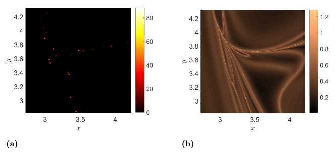
(a)

(b)

Figure 14: Steady ABC flow: Error due to finite differencing. (a) Angle in degrees between $\xi_{2}$ obtained from finite differencing of $F_{t_{0}}^{t_{1}}$ (cf. (Haller2015, )) and $\xi_{2}$ obtained using the equation of variations (30). (b) FTLE $(t_{1}-t_{0})^{-1}\log\sigma_{3}$ obtained using the equation of variations (30).

In Fig. 14a, we show the angle between $\xi_{2}$ obtained using (30) and $\xi_{2}$ obtained from finite differencing of $F_{t_{0}}^{t_{1}}$. The former method can be considered practically exact here, with the only numerical parameter being $Tol=10^{-8}$ (checked for convergence). The largest error we find in Fig. 14a is approximately $88.35{{}^{\circ}}$. Since $\xi_{2}$ is only defined up to orientation, the largest possible error would be $90{{}^{\circ}}$. Hence we conclude from Fig. 14a that finite differencing can cause arbitrarily large errors in $\xi_{2}$. Even though errors are confined to locations of exceptionally large separation, as indicated by the finite-time Lyapunov exponent (FTLE) field (cf. Fig. 14b), these locations belong to ridges of the FTLE field, a widely used indicator of hyperbolic LCSs (Haller2015, ). Since we want to globally detect hyperbolic LCSs by integrating the $\xi_{2}$-field, we use (30) to determine $\xi_{2}$.

We note that even when the velocity field (1) is only available through data from experiments and simulations, the equation of variations (30) has been used to obtain numerically accurate results for the flow map and its gradient (Miron20126419, ).

Appendix D Perturbations to the $\xi_{2}$-field

In Figs. 11a, 11b, we place a tracer sphere in an LCS candidate surface, finding that it stretches most in the direction normal to the surface. Based on this local property, in Sec. V.3, we conclude that the entire surface should be a repelling LCS. Even though we expect any hyperbolic LCS obtained from a forward-time computation to be repelling (cf. Remark 6), it is desirable to have a global approach to assessing the LCS type of a candidate surface.

If we consider, e.g., a repelling LCS $\mathcal{M}(t_{0})$, at any point $x_{0}\in\mathcal{M}(t_{0})$, the tangent space $T_{x_{0}}\mathcal{M}(t_{0})$ is the subspace of $\mathbb{R}^{3}$ spanned by $\xi_{2}(x_{0})$ and $\xi_{1}(x_{0})$ (cf. Proposition 1). By repeating the reasoning that leads to Theorem 1, we conclude that any repelling LCS $\mathcal{M}(t_{0})$ must be an invariant manifold of any dynamical system of the form

$$x_{0}^{\prime}=p\,\xi_{2}(x_{0})+(1-p)\xi_{1}(x_{0}),\quad p\in[0,1].$$

By Propositions 2–4, we can make similar observations for the remaining LCS types. In summary:

Proposition 5.

For any parameter value $p\in[0,1]$, the initial position $\mathcal{M}(t_{0})$ of any hyperbolic or elliptic LCS (Definitions 2–4) is an invariant manifold of the autonomous dual dynamical system

$$x_{0}^{\prime}=p\,\xi_{2}(x_{0})+(1-p)\tilde{\xi}(x_{0})\,,$$ (31)

with $\mbox{$\tilde{\xi}$=$\xi$}_{3}$ for attracting hyperbolic LCSs; $\tilde{\xi}=\xi_{1}$ for repelling hyperbolic LCSs; and $\tilde{\xi}=\mp\tilde{\gamma}\xi_{1}+\tilde{\alpha}\xi_{3}$ or $\tilde{\xi}=\mp\gamma\xi_{1}+\alpha\xi_{3}$ for elliptic LCSs (cf. (11), (12)).

Remark 7.

Replacing the $\xi_{1,2,3}$ by $\sigma_{1,2,3}\cdot\eta_{1,2,3}$, Proposition 5 applies verbatim to final LCS positions $\mathcal{M}(t_{1})$.

This means that for each LCS type, there is a specific family of dual dynamical systems that yields the respective LCS initial positions as invariant manifolds. The dual dynamical system associated with $\xi_{2}$ remains exceptional though, because this is the only dual dynamical system shared by all LCS types (cf. Proposition 5).

We now demonstrate how these observations help to determine the LCS type of a candidate surface: For the hyperbolic LCS candidate in the time-aperiodic ABC-type flow (cf. Sec. V.3), it turns out that only a single long $\xi_{2}$-line is enough to indicate the surface (cf. Fig. 15a). Specifically, among the $\xi_{2}$-lines that get attracted to the hyperbolic LCS candidate surface in the dual Poincaré map (cf. Fig. 9a), we have randomly picked the $\xi_{2}$-line with initial condition approximately equal to $(5.03,3.14,0.00)$. Other choices of $\xi_{2}$-lines yield similar results.

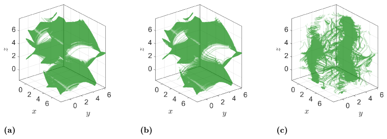
(a)

(b)

(c)

Figure 15: Time-aperiodic ABC-type flow: Arc segments of integral curves of three $\xi_{2}+\epsilon\tilde{\xi}$ fields. (Each curve is shown for arclength parameter $s\in[4\cdot 10^{4},5\cdot 10^{4}]$). The initial condition is approximately $(5.03,3.14,0.00)$ for all three integral curves. Here we use the periodicity of the phase space to extend the domain slightly beyond $[0,2\pi]^{3}$. (a) A $\xi_{2}$-line ($\epsilon=0$) indicates the hyperbolic candidate surface obtained from the dual Poincaré map (cf. Fig. 9a). (b) An integral curve of $\xi_{2}+\epsilon\xi_{1}$ ($\epsilon=0.01$) reproduces the hyperbolic candidate surface obtained from the corresponding $\xi_{2}$-line (cf. Fig. 15a). (c) An integral curve of $\xi_{2}+\epsilon\xi_{3}$ ($\epsilon=0.01$) does not reproduce the hyperbolic candidate surface obtained from the corresponding $\xi_{2}$-line (cf. Fig. 15a).

We next add a small perturbation to the $\xi_{2}$-field, i.e., consider the dual dynamical system

$$x_{0}^{\prime}=\xi_{2}(x_{0})+\epsilon\xi_{1}(x_{0}),$$ (32)

with $\epsilon=0.01$. Using the same initial condition and numerical settings as above, we compute an integral curve of (32). The result indicates virtually the same surface as obtained from the $\xi_{2}$-field (cf. Fig. 15b). This suggests that this surface is invariant for the entire family of direction fields $p\xi_{2}+(1-p)\xi_{1}$. By Proposition 5, the entire structure should hence be a repelling LCS.

If we, on the other hand, repeat the above computation for the dual dynamical system

$$x_{0}^{\prime}=\xi_{2}(x_{0})+\epsilon\xi_{3}(x_{0}),$$ (33)

where $\epsilon=0.01$, then the entire structure disappears, and the attractor for this initial condition remains unclear (cf. Fig. 15c). Even though the perturbation $\epsilon\xi_{3}$ is small, the dynamics of (33) is completely different than for (32). This is consistent with our conclusion that the structure from Figs. 15a, 15b is a repelling hyperbolic LCS.

References

- [1] V. I. Arnold. Mathematical Methods of Classical Mechanics, pages 271–300. Springer, 1989. (Second edition).
- [2] D. Blazevski and G. Haller. Hyperbolic and elliptic transport barriers in three-dimensional unsteady flows. Physica D, 273-274:46 – 62, 2014.
- [3] J. R. Dormand and P. J. Prince. A family of embedded Runge-Kutta formulae. J. Comput. Appl. Math., 6(1):19–26, 1980.
- [4] M. Farazmand, D. Blazevski, and G. Haller. Shearless transport barriers in unsteady two-dimensional flows and maps. Physica D, 278-279:44–57, Jun 2014.
- [5] M. Farazmand and G. Haller. Attracting and repelling Lagrangian coherent structures from a single computation. Chaos, 23(2):023101, 2013.
- [6] M. Farazmand and G. Haller. Polar rotation angle identifies elliptic islands in unsteady dynamical systems. Physica D, 315:1–12, 2016.
- [7] V. Guillemin and A. Pollack. Differential topology. Prentice-Hall, 1974.
- [8] G. Haller. A variational theory of hyperbolic Lagrangian Coherent Structures. Physica D, 240(7):574–598, Mar 2011.
- [9] G. Haller. Lagrangian Coherent Structures. Annual Review of Fluid Mechanics, 47(1):137–162, 2015.
- [10] G. Haller and F. J. Beron-Vera. Coherent Lagrangian vortices: the black holes of turbulence. J. Fluid Mech., 731:R4 (10 pages), Sep 2013.
- [11] G. Haller, A. Hadjighasem, M. Farazmand, and F. Huhn. Defining coherent vortices objectively from the vorticity. In press, J. Fluid Mech., 2016.
- [12] G. Haller and T. Sapsis. Lagrangian coherent structures and the smallest finite-time Lyapunov exponent. Chaos, 21(2):023115, 2011.
- [13] D. Karrasch. Attracting Lagrangian Coherent Structures on Riemannian Manifolds. Chaos, 25(8):087411, 2015.
- [14] D. Karrasch, M. Farazmand, and G. Haller. Attraction-based computation of hyperbolic Lagrangian coherent structures. Journal of Computational Dynamics, 2(1):83–93, 2015.
- [15] B. Krauskopf, H. M. Osinga, E. J. Doedel, M. E. Henderson, J. Guckenheimer, A. Vladimirsky, M. Dellnitz, and O. Junge. A survey of methods for computing (un) stable manifolds of vector fields. IJBC, 15(03):763–791, 2005.
- [16] J. M. Lee. Introduction to Smooth Manifolds, pages 491–493. Springer, 2012.
- [17] A. J. Majda and A. L. Bertozzi. Vorticity and incompressible flow, pages 54–59. Cambridge University Press, 2002.
- [18] J. E. Marsden and T. J. R. Hughes. Mathematical Foundations of Elasticity, page 50. Dover, 1994.
- [19] P. Miron, J. Vétel, A. Garon, M. Delfour, and M. E. Hassan. Anisotropic mesh adaptation on Lagrangian Coherent Structures. J. Comput. Phys, 231(19):6419 – 6437, 2012.
- [20] D. Oettinger, D. Blazevski, and G. Haller. Global variational approach to elliptic transport barriers in three dimensions. Chaos, 26(3):033114, 2016.
- [21] L. N. Trefethen and D. Bau III. Numerical Linear Algebra, volume 50, pages 25–37. SIAM, 1997.
- [22] D. S. Watkins. Product eigenvalue problems. SIAM Review, 47(1):3–40, 2005.