Scattering and bound states of a spin–1/2 neutral particle in the cosmic string spacetime

Abstract

In this paper the relativistic quantum dynamics of a spin-1/2 neutral particle with a magnetic moment $\mu$ in the cosmic string spacetime is reexamined by applying the von Neumann theory of self–adjoint extensions. Contrary to previous studies where the interaction between the spin and the line of charge is neglected, here we consider its effects. This interaction gives rise to a point interaction: $\boldsymbol{\nabla}\cdot\mathbf{E}=(2\lambda/\alpha)\delta(r)/r$. Due to the presence of the Dirac delta function, by applying an appropriated boundary condition provided by the theory of self–adjoint extensions, irregular solutions for the Hamiltonian are allowed. We address the scattering problem obtaining the phase shift, S-matrix and the scattering amplitude. The scattering amplitude obtained shows a dependency with energy which stems from the fact that the helicity is not conserved in this system. Examining the poles of the S-matrix we obtain an expression for the bound states. The presence of bound states for this system has not been discussed before in the literature.

I Introduction

Theory of topological defects is a natural framework for studying properties of physical systems. In cosmology, the origin of defects can be understood as a sequence of phase transitions in the early universe. These processes occur with critical temperatures which are related to the corresponding symmetry spontaneously breaking scales Dolan and Jackiw (1974); Weinberg (1974); Linde (1979). These phase transitions can give rise to topologically stable defects, for example, domain walls, strings and monopoles Kibble (1976). Topological defects are also found in condensed matter systems. In these systems, they appears as vortices in superconductors, domain wall in magnetic materials, dislocations of crystalline substances, among others. An important property that can be verified in topological defects is that they are described by a spacetime metric with a Riemann–Christoffel curvature tensor which is null everywhere except on the defects. Here, we look for a cosmic string, which is a linear topological defect with a conical singularity at the origin. The interest in this subject has contributed to the understanding and advancement of other physical phenomena occurring in the universe and also in the context of non-relativistic physics. For example, in the galaxy formation Silk and Vilenkin (1984); Turok and Brandenberger (1986), to study vortex solutions in non-abelian gauge theories with spontaneous symmetry breaking Manías et al. (1986) and to study the gravitational analogue of the Aharonov–Bohm effect Dowker (1967); Ford and Vilenkin (1981); Stachel (1982); Bezerra (1987); Aliev and Gal’tsov (1989). In recent developments, cosmic strings have been considered to analyze solutions in de Sitter and anti-de Sitter spacetimes de Pádua Santos and Bezerra de Mello (2016), to study the thermodynamic properties of a neutral particle in a magnetic cosmic string background by using an approach based on the partition function method Hassanabadi and Hosseinpour (2016), to compute the vacuum polarization energy of string configurations in models similar to the standard model of particle physics Weigel et al. (2016), to find the deflection angle in the weak limit approximation by a spinning cosmic string in the context of the Einstein–Cartan theory of gravity Jusufi (2016), to analyze numerically the behavior of the solutions corresponding to an Abelian string in the framework of the Starobinsky model Graça (2016), to study solutions of black holes Vieira et al. (2015), to investigate the average rate of change of energy for a static atom immersed in a thermal bath of electromagnetic radiation Cai et al. (2015), to study Hawking radiation of massless and massive charged particles Jusufi (2015), to study the non-Abelian Higgs model coupled with gravity de Pádua Santos and Bezerra de Mello (2015), in the quantum dynamics of scalar bosons Castro (2015), hydrodynamics Beresnyak (2015), to study the non-relativistic motion of a quantum particle subjected to magnetic field Hassanabadi et al. (2015), to investigate dynamical solutions in the context of super–critical tensions Niedermann and Schneider (2015), Higgs condensate Mota and Hindmarsh (2015), to analyze the effects on spin current and Hall electric field Wang et al. (2013); Chowdhury and Basu (2014), to investigate the dynamics of the Dirac oscillator Carvalho et al. (2011); Andrade and Silva (2014), to study non-inertial effects on the ground state energy of a massive scalar field Mota and Bakke (2014), Landau quantization Muniz et al. (2014) and to investigate the quantum vacuum interaction energy M. Muñoz Castañeda and Bordag (2014).

In the present work, we study the quantum dynamics of a spin–1/2 neutral particle in the presence of an electric field due to an infinitely long, infinitesimally thin line of charge along the $z$–axis of the cosmic string, with constant charge density on it. This model have been studied in Ref. Bezerra de Mello (2004) in the non-relativistic regime and, for this particular case, only the scattering problem was considered. The present system is an adaptation of the usual Aharonov-Casher problem Aharonov and Casher (1984) (which is dual to the Aharonov-Bohm problem Aharonov and Bohm (1959)), where now effects of localized curvature are included in the model. We reexamine this problem by using the von Neumann theory of self–adjoint extensions Bulla and Gesztesy (1985); Albeverio et al. (2004). We address the relativistic case and investigate some questions that were not considered in the previous studies, as for example, the existence of bound states. For this, we solve the scattering problem and derive the $S$ matrix in order to obtain such bound states.

The plan of this work is the following. In Section II, we derive the Dirac-Pauli equation in the cosmic string spacetime without neglecting the term which depends explicitly on the spin. Arguments based on the theory of self–adjoint extension are given in order to make clear the reasons why we should consider the spin effects in the dynamics of the system. In Section III, we study the Dirac–Pauli Hamiltonian via the von Neumann theory of self–adjoint extension. We address the scattering scenario within the framework of Dirac–Pauli equation. Expressions for the phase shift, S-matrix, and bound states are derived. We also make an investigation on the helicity conservation problem in the present framework. A brief conclusion is outlined in Section IV.

II The relativistic equation of motion

The model that we address here consists of a spin–1/2 neutral particle with mass $M$ and magnetic moment $\mu$, moving in an external electromagnetic field $F_{\mu\nu}$ in the cosmic string spacetime, described by the line element in cylindrical coordinates,

$$ds^{2}=c^{2}dt^{2}-dr^{2}-\alpha^{2}r^{2}d\varphi^{2}-dz^{2},$$ (1)

with $-\infty<(t,z)<\infty$, $r\geq 0$, $0\leq\varphi\leq 2\pi$ and $\alpha$ is given in terms of the linear mass density $\tilde{m}$ of the cosmic string by $\alpha=1-4\tilde{m}/c^{2}$. This metric has a cone-like singularity at $r=0$ Sokolov and Starobinski (1977). In this system, the fermion particle is described by a four–component spinorial wave function $\Psi$ obeying the generalized Dirac–Pauli equation in a non flat spacetime, which should include the spin connection in the differential operator. Moreover, in order to make the Dirac–Pauli equation valid in curved spacetime, we must rewrite the standard Dirac matrices, which are written in terms of the local coordinates in the Minkowski spacetime, in terms of global coordinates. This can be accomplished by using the inverse vierbeins $e_{\bar{a}}^{\mu}$ through the relation $\gamma^{\mu}=e_{\bar{a}}^{\mu}\gamma^{\bar{a}}$ $(\mu,\bar{a}=0,1,2,3)$, with $\gamma^{\bar{a}}=\left(\gamma^{\bar{0}},\gamma^{\bar{i}}\right)$ being the standard gamma matrices. The equation of motion governing the dynamics of this system is the modified Dirac–Pauli equation in the curved space

$$\left[i\hbar\gamma^{\mu}\left(\partial_{\mu}+\Gamma_{\mu}\right)-\frac{\mu}{2c}\sigma^{\mu\nu}F_{\mu\nu}-Mc\right]\Psi=0,$$ (2)

with $\sigma^{\mu\nu}={}i[\gamma^{\mu},\gamma^{\nu}]/2$, $\left(F_{0i},F_{ij}\right)={}\left(E^{i},\epsilon_{ijk}B^{k}\right)$, $\left(\sigma^{0j},\sigma^{ij}\right)={}\left(i\alpha^{j},-\epsilon_{ijk}\Sigma^{k}\right)$, where $E^{i}$ and $B^{k}$ are the electric and magnetic field strengths and $\Sigma^{k}$ is the spin operator. Here, we use the same vierbein of the Ref. Bakke et al. (2008), where the spinorial affine connection $\Gamma_{\mu}$ has been calculated in detail. Moreover, in this work, we are only interested on the planar dynamics of a spin–1/2 neutral particle under the action of a radial electric field. In this manner we require that $p_{z}=z=0$ and $B^{k}=0$ for $k=1,2,3$. Furthermore, according to the tetrad postulated Lawrie (2012), the matrices $\gamma^{\bar{a}}$ can be any set of constant Dirac matrices in a such way that we are free to choose a representation for them. We choose to work in a representation in which the Dirac matrices are given in terms of the Pauli matrices, namely Brandenberger et al. (1988); Alford et al. (1989)

$$\beta=\gamma^{\bar{0}}=\sigma^{3},\qquad\gamma^{\bar{1}}=i\sigma^{2},\qquad\gamma^{\bar{2}}=-is\sigma^{1},$$ (3)

where $(\sigma^{1},\sigma^{2},\sigma^{3})$ are the Pauli matrices and $s$ is twice the spin value, with $s=+1$ for spin “up” and $s=-1$ for spin “down”. In this representation, the only non-vanishing component of the spinorial affine connection $\Gamma_{\mu}$ is found to be

$$\Gamma_{\varphi}=-i\frac{\left(1-\alpha\right)}{2}s\sigma^{z}.$$ (4)

For the field configuration, we consider the electric field due to a linear charge distribution, superposed to the cosmic string. The expression for this field is seem to be

$$E_{r}=\frac{2\lambda}{\alpha r}.$$ (5)

Therefore, the second order equation associated with Eq. (2) reads

$$\hat{H}\Phi=k^{2}\Phi,$$ (6)

with

$$\hat{H}={} -\nabla_{\alpha}^{2}-\frac{(1-\alpha)s\sigma^{z}}{i\alpha^{2}r^{2}}\partial_{\varphi}+\frac{(1-\alpha)^{2}}{4\alpha^{2}r^{2}}+\frac{2\mu s}{\hbar c}\frac{E_{r}}{i\alpha r}\partial_{\varphi}$$

$$+\frac{\mu}{\hbar c}(\partial_{r}E_{r})\sigma^{z}-\frac{\mu}{\hbar c}\frac{(1-\alpha)E_{r}}{\alpha r}\sigma^{z}+\frac{\mu^{2}}{\hbar^{2}c^{2}}E_{r}^{2},$$ (7)

where $\nabla_{\alpha}^{2}=\partial_{r}^{2}+(1/r)\partial_{r}+(1/\alpha^{2}r^{2})\partial_{\varphi}^{2}$ is the Laplace-Beltrami operator in the conical space and $k^{2}=\left(\mathcal{E}^{2}-M^{2}c^{4}\right)/\hbar^{2}c^{2}$. As the angular momentum $\hat{J}=-i\partial_{\varphi}+(s/2)\sigma^{z}$, commutes with the $\hat{H}$, it is possible to decompose the fermion field as

$$\Phi=\begin{pmatrix}\psi\\ \chi\end{pmatrix}=\begin{pmatrix}\sum_{m}f_{m}(r)\,e^{im\varphi}\\ \sum_{m}g_{m}(r)\,e^{i\left(m+s\right)\varphi}\end{pmatrix},$$ (8)

where $m=0,\pm 1,\pm 2,\pm 3,\ldots$ is the angular momentum quantum number. In this manner, the radial equation for $f_{m}(r)$ is

$$hf_{m}(r)=k^{2}f_{m}(r),$$ (9)

with

$$h=h_{0}+\frac{\eta}{\alpha}\frac{\delta(r)}{r},$$ (10)

and

$$h_{0}=-\frac{d^{2}}{dr^{2}}-\frac{1}{r}\frac{d}{dr}+\frac{j^{2}}{r^{2}},$$ (11)

where

$$j=\frac{m+s\eta}{\alpha}-\frac{s(1-\alpha)}{2\alpha},$$ (12)

is the effective angular momentum and

$$\eta=\frac{\phi}{\phi_{0}}.$$ (13)

Here, $\phi=4\pi\lambda$ is the electric flux of the electric field and $\phi_{0}=hc/\mu$ is the quantum of electric flux.

As far as we know, only the scattering problem for the Hamiltonian in Eq. (10) has been studied in Ref. Bezerra de Mello (2004). However, there, the spin effect was not taken into account once the author imposed the regularity of the wave function at the origin. The inclusion of spin gives rise to the Dirac delta function potential, which comes from the interaction between the spin and the line of charge, and its inclusion has effects on the scattering phase shift, giving rise to an additional scattering phase shift Hagen (1990a). Thus, the main aim of this work is to show that there are bound states due to the presence of the Dirac delta function. The approach adopted here is that of the self–adjoint extensions Albeverio et al. (2004), which has been used to deal with singular Hamiltonians, for instance, in the study of spin 1/2 Aharonov-Bohm system and cosmic strings Khalilov (2014); de Sousa Gerbert (1989), in the Aharonov-Bohm-Coulomb problem Khalilov (2013); Khalilov and Mamsurov (2009); Park and Oh (1994); Park (1995), and in the equivalence between the self–adjoint extension and normalization Jackiw (1995).

III Scattering and bound states analysis

In this section, we obtain the S-matrix and from its poles an expression for the bound states is obtained. Before we solve Eq. (9), let us first analyze the Hamiltonian $h_{0}$.

In the von Neumann theory of self–adjoint extensions, a Hermitian operator $\hat{O}$ ($\hat{O}=\hat{O}^{\dagger}$) defined in a dense subset of a Hilbert space has deficiency indices $(n_{+},n_{-})$, which are the sizes of the deficiency sub-spaces spanned by the solutions for

$$\hat{O}\chi_{\pm}=\pm i\chi_{\pm}.$$ (14)

When the dimension of the deficiency subspace are zero, the operator is self–adjoint and it has no additional self–adjoint extension. When the dimension of the deficiency spaces are not zero the operator is not self–adjoint. If $n_{+}=n_{-}=n$ the operator admits a self–adjoint extension parametrized by a $n\times n$ unitary matrix. However, if the deficiency indices are not equal, the operator has no self–adjoint extensions. By standard results, it is well-known that the Hamiltonian $h_{0}$ has deficiency indices $(1,1)$ and it is self–adjoint for $|j|\geq 1$, whereas for $|j|<1$ it is not self–adjoint, and admits an one-parameter family of self–adjoint extensions Reed and Simon (1975). Actually, $h$ can be interpreted as a self–adjoint extension of $h_{0}$ Gesztesy et al. (1987). All the self–adjoint extension of $h_{0}$, $h_{0,\nu}$, are accomplished by requiring the boundary condition at the origin Bulla and Gesztesy (1985)

$$\nu f_{0,j}=f_{1,j},$$ (15)

where $-\infty<\nu\leq\infty$ and $-1<j<1$. The boundary values are

$$f_{0,j}={} \lim_{r\to 0^{+}}r^{|j|}f_{m}(r),$$

$$f_{1,j}={} \lim_{r\to 0^{+}}\frac{1}{r^{|j|}}\left[f_{m}(r)-f_{0,j}\frac{1}{r^{|j|}}\right].$$

In Eq. (15) $\nu$ is the self–adjoint extension parameter. It turns out that $1/\nu$ represents the scattering length of $h_{0,\nu}$ Albeverio et al. (2004). For $\nu=\infty$ (the Friedrichs extension of $h_{0}$), one has the free Hamiltonian (without spin) with regular wave functions at the origin ($f_{m}(0)=0$). This situation is equivalent to impose the Dirichlet boundary condition on the wave function. On the other hand, if $|\nu|<\infty$, $h_{0,\nu}$ describes a point interaction at the origin. In this latter case the boundary condition permits a $r^{-|j|}$ singularity in the wave functions at the origin Hagen (2008).

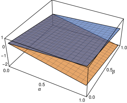
Figure 1: In this figure we plot the planes $\pi_{-}(\alpha,\beta)$ (orange, bottom) and $\pi_{+}(\alpha,\beta)$ (blue, top) for $N=0$ and $s=+1$. The region between the two planes is that in which the operator $h_{0}$ is not self–adjoint.

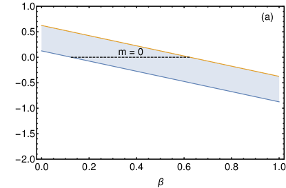
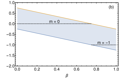
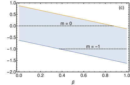
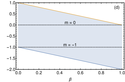
Figure 2: Cross sections of Fig. 1 for different values of the deficit angle: (a) $\alpha=0.25$, (b) $\alpha=0.50$, (c) $\alpha=0.75$ and (d) $\alpha=1.00$. The shaded area schematically represents that area in which the operator $h_{0}$ is not self–adjoint. The dashed lines represent the values of angular moment quantum number.

Let us now discuss for which values of the angular moment quantum number $m$, the operator $h_{0}$ is not self–adjoint. In fact, these values depending on the variables $\alpha$ and $\eta$. As discussed in Bezerra de Mello (2004), $0<\alpha<1$ represents a positive curvature and a planar deficit angle, corresponding to a conical spacetime. On the other hand, $\alpha>1$ represents a negative curvature and an excess of planar angle, corresponding to an anti-conical spacetime. Finally, $\alpha=1$ corresponds to a flat space. Then, we focus on a conical spacetime. For the electric flux $\eta$ let us adopt the decomposition defined by Hagen (1990b)

$$\eta=N+\beta,$$ (16)

being $N$ an integer and

$$0\leq\beta<1.$$ (17)

The inequality $|j|<1$ then reads

$$\pi_{-}(\alpha,\beta)<m<\pi_{+}(\alpha,\beta),$$ (18)

with $\pi_{\pm}(\alpha,\beta)=\pm\alpha-[(2\beta+\alpha-1)s/2-sN]$. In Fig. 1 we plot the planes $\pi_{\pm}(\alpha,\beta)$ for $N=0$ and $s=+1$. The region between these two planes is that in which the operator $h_{0}$ is not self–adjoint. In Fig. 2 we show cross sections of this region for some particular values of the deficit angle $\alpha$. We can observe in Fig. 2(a) that, for $\alpha=0.25$, only for $m=0$ the operator $h_{0}$ is not self adjoint, whereas for $\alpha=0.50$ (Fig. 2(b)) the operator $h_{0}$ is not self adjoint for $m=0$ and $m=-1$, but not for both values of $m$ at same time for the whole range of $\beta$ values. Indeed, a necessary condition for the operator $h_{0}$ not being self–adjoint for the state with $m=-1$ is $\alpha>1-2\beta/3$. In fact, this condition is also valid for $N\neq 0$ and, in this latter case, the $m$ values for which the $h_{0}$ is not self–adjoint are shifted to the values $sN$ and $sN-1$. For $\alpha=0.75$ (Fig. 2(c)) we can observe that there is a range the values of $\beta$ in which, for both values of $m=0$ and $m=-1$, the operator $h_{0}$ is not self–adjoint. And last but not least, $\alpha=1.0$ (see Fig 2 (d)) is the only situation in which the operator $h_{0}$ is not self–adjoint for the both values of angular momentum quantum number for the whole range of $\beta$ (the unique exception is $\beta=0$).

Now, let us comeback to the solution of Eq. (9). As a matter of fact, it is the Bessel differential equation. Thus, the general solution for $r\neq 0$ is seen to be

$$f_{m}(r)=a_{m}J_{|j|}(kr)+b_{m}J_{-|j|}(kr),$$ (19)

where $J_{\nu}(z)$ is the Bessel function of fractional order. The coefficients $a_{m}$ and $b_{m}$ represent the contributions of the regular and irregular solutions at the origin, respectively. Thus making use of the boundary condition in Eq. (15) in the subspace $|j|<1$, a relation between the coefficients is obtained, namely,

$$b_{m}=-\mu_{\nu}a_{m},$$ (20)

where the term $\mu_{\nu}$ is given by

$$\mu_{\nu}=\frac{k^{2|j|}\Gamma(1-|j|)\sin(|j|\pi)}{4^{|j|}\Gamma(1+|j|)\nu+k^{2|j|}\Gamma(1-|j|)\cos(|j|\pi)},$$ (21)

where $\Gamma(z)$ is the gamma function. Therefore, in this subspace the solution reads

$$f_{m}(r)=a_{m}\left[J_{|j|}(kr)-\mu_{\nu}J_{-|j|}(kr)\right].$$ (22)

The above equation shows that the self–adjoint extension parameter $\nu$ controls the contribution of the irregular solution $J_{-|j|}$ for the wave function. As a result, for $\nu=\infty$, we have $\mu_{\infty}=0$, and there is no contribution of the irregular solution at the origin for the wave function. Consequently, the total wave function reads

$$\psi=\sum_{m=-\infty}^{\infty}a_{m}J_{|j|}(kr)e^{im\varphi}.$$ (23)

It is well-known that the coefficient $a_{m}$ must be chosen in a such way that $\psi$ represents a plane wave that is incident from the right. In this manner, we obtain the result

$$a_{m}=e^{-i|j|\pi/2}.$$ (24)

The scattering phase shift can be obtained from the asymptotic behavior of Eq. (23). This leads to

$$\delta_{m}=\frac{\pi}{2}(|m|-|j|).$$ (25)

This is the scattering phase shift of the Aharonov-Casher effect in the cosmic string background. It is worthwhile to note that, for $\alpha=1$, it reduces to the phase shift for the usual Aharonov-Casher effect in flat space $\delta_{m}=\pi(|m|-|m+s\eta|)/2$ Aharonov and Casher (1984).

On the other hand, for $|\nu|<\infty$, the contribution of the irregular solution modifies the scattering phase shift to

$$\delta_{m}^{\nu}=\delta_{m}+\arctan(\mu_{\nu}).$$ (26)

Thus one obtains

$$S_{m}^{\nu}=e^{2i\delta_{m}^{\nu}}=e^{2i\delta_{m}}\left(\frac{1+i\mu_{\nu}}{1-i\mu_{\nu}}\right),$$ (27)

which is the expression for the S-matrix in terms of the phase shift. As a result, one observes that in this latter case there is an additional scattering for any value of the self–adjoint extension parameter $\nu$. When $\nu=\infty$, we have the S-matrix for the Aharonov-Casher effect on the cosmic string background, as it should be.

The S-matrix or scattering matrix relates incoming and outgoing wave functions of a physical system undergoing a scattering process. Bound states are identified as the poles of the S-matrix in the upper half in the complex $k$ plane. In this manner, the poles are determined at the zeros of the denominator in Eq. (27) with the replacement $k\rightarrow i\kappa$ with $\kappa=\sqrt{-\left(\mathcal{E}^{2}-M^{2}c^{4}\right)/\hbar^{2}c^{2}}$. Therefore, for $\nu<0$, one can determine that the present system has a bound state with energy given

$$\mathcal{E}=\pm\sqrt{M^{2}c^{4}-4\hbar^{2}c^{2}\left[-\nu\frac{\Gamma(1+|j|)}{\Gamma(1-|j|)}\right]^{1/|j|}}.$$ (28)

and the normalized radial bound state wave function is

$$\begin{pmatrix}f_{m}(r)\\ g_{m}(r)\end{pmatrix}={} \sqrt{\frac{2\alpha\kappa^{2}/\pi}{|j|\alpha\csc(|j|\pi)+|j^{\prime}|\csc(|j^{\prime}|\pi)}}$$

$$\times\begin{pmatrix}K_{|j|}(\kappa r)\\ K_{|j^{\prime}|}(\kappa r)\end{pmatrix},$$ (29)

where $j^{\prime}=j+(s/\alpha)(2-\alpha)$ and $K_{\nu}(z)$ is the modified Bessel function of the second kind. So, there are bound states when the self–adjoint extension parameter is negative. In the non-relativistic limit and for $\alpha=1$, Eq. (28) coincides with the bound state energy found in Ref. Silva et al. (2013) for the Aharonov-Casher effect in the flat space.

As a result, it is possible to express the S-matrix in terms of the bound state energy. The result is seem to be

$$S_{m}^{\nu}=e^{2i\delta_{m}}\left[\frac{e^{2i\pi|j|}-(\kappa/k)^{2|j|}}{1-(\kappa/k)^{2|j|}}\right].$$ (30)

Once we have obtained the S-matrix, it is possible to write down the scattering amplitude $f(k,\varphi)$. The result is

$$f(k,\varphi)={} \frac{1}{\sqrt{2\pi ik}}\sum_{m=-\infty}^{\infty}\left(S_{m}^{\nu}-1\right)e^{im\varphi}$$

$$={} \frac{1}{\sqrt{2\pi ik}}\Bigg{\{}\sum_{m\in\{|j|\geq 1\}}\left(e^{2i\delta_{m}}-1\right)e^{im\varphi}$$

$$+\sum_{m\in\{|j|<1\}}\left[e^{2i\delta_{m}}\left(\frac{1+i\mu_{\nu}}{1-i\mu_{\nu}}\right)-1\right]e^{im\varphi}\Bigg{\}}.$$ (31)

In scattering problems the length scale is set by $1/k$, thus the scattering amplitude $f(k,\varphi)$ would be a function of angle alone, multiplied by $1/k$ Goldhaber (1977). However, we observe that $f(k,\varphi)$ has a dependence on $\mu_{\nu}$, which in its turn has explicit dependence on $k$ (see Eq. (21)). This behavior is associated with the failure of helicity conservation. The helicity operator, defined by

$$\hat{h}=\boldsymbol{\Sigma}\cdot(-i\boldsymbol{\nabla}_{\alpha}-e\mathbf{A}),$$ (32)

obeys the equation

$$\frac{d\hat{h}}{dt}=e\boldsymbol{\Sigma}\cdot\mathbf{E},$$ (33)

whit $\boldsymbol{\Sigma}$ is the spin operator and in Eq. (32) $\mathbf{A}$ is the potential vector, which is absent in the present problem. Therefore, due to the presence of electric field the helicity is not conserved.

IV Conclusions

In this work, we reexamined the relativistic quantum dynamics of a spin–1/2 neutral particle in the cosmic string spacetime. This problem has been studied in Ref. Bezerra de Mello (2004) in the non-relativistic scenario. However only the scattering solutions were studied and without taking into account the possibility of bound states. Here, we have showed that the inclusion of electron spin, which gives rise to a point interaction, changes the scattering phase shift and consequently the S-matrix. The results were obtained by imposing the boundary condition in Eq. (15), which comes from the von Neumann theory of the self–adjoint extensions. Our results are dependent on the self–adjoint extension parameter $\nu$. For the special value of $\nu=\infty$ we recover the results of Ref. Bezerra de Mello (2004). Our expression for the scattering amplitude has an energy dependency. So, the helicity is not conserved in the scattering process. Last but not least, examining the poles of the S-matrix, an expression for the bound state energy was determined. The presence of bound states has not been discussed before.

Conflict of interest

The authors declare that there is no conflict of interests regarding the publication of this paper.

References

- Dolan and Jackiw (1974) L. Dolan and R. Jackiw, Phys. Rev. D 9, 3320 (1974).
- Weinberg (1974) S. Weinberg, Phys. Rev. D 9, 3357 (1974).
- Linde (1979) A. D. Linde, Rep. Prog. Phys. 42, 389 (1979).
- Kibble (1976) T. W. B. Kibble, J. Phys. A: Math. Gen. 9, 1387 (1976).
- Silk and Vilenkin (1984) J. Silk and A. Vilenkin, Phys. Rev. Lett. 53, 1700 (1984).
- Turok and Brandenberger (1986) N. Turok and R. H. Brandenberger, Phys. Rev. D 33, 2175 (1986).
- Manías et al. (1986) M. Manías, C. Naón, F. Schaposnik, and M. Trobo, Phys. Lett. B 171, 199 (1986).
- Dowker (1967) J. S. Dowker, Il Nuovo Cimento B Series 10 52, 129 (1967).
- Ford and Vilenkin (1981) L. H. Ford and A. Vilenkin, J.Phys. A: Math. Gen. 14, 2353 (1981).
- Stachel (1982) J. Stachel, Phys. Rev. D 26, 1281 (1982).
- Bezerra (1987) V. B. Bezerra, Phys. Rev. D 35, 2031 (1987).
- Aliev and Gal’tsov (1989) A. Aliev and D. Gal’tsov, Ann. Phys. 193, 142 (1989).
- de Pádua Santos and Bezerra de Mello (2016) A. de Pádua Santos and E. R. Bezerra de Mello, Phys. Rev. D 94, 063524 (2016).
- Hassanabadi and Hosseinpour (2016) H. Hassanabadi and M. Hosseinpour, The European Physical Journal C 76, 553 (2016).
- Weigel et al. (2016) H. Weigel, M. Quandt, and N. Graham, Phys. Rev. D 94, 045015 (2016).
- Jusufi (2016) K. Jusufi, The European Physical Journal C 76, 332 (2016).
- Graça (2016) J. P. M. Graça, Classical and Quantum Gravity 33, 055004 (2016).
- Vieira et al. (2015) H. Vieira, V. Bezerra, and G. Silva, Ann. Phys. 362, 576 (2015).
- Cai et al. (2015) H. Cai, H. Yu, and W. Zhou, Phys. Rev. D 92, 084062 (2015).
- Jusufi (2015) K. Jusufi, Gen. Relativ. Gravitation 47, 1 (2015).
- de Pádua Santos and Bezerra de Mello (2015) A. de Pádua Santos and E. R. Bezerra de Mello, Class. Quantum Grav. 32, 155001 (2015).
- Castro (2015) L. B. Castro, Eur. Phys. J. C 75, 287 (2015).
- Beresnyak (2015) A. Beresnyak, The Astrophysical Journal 804, 121 (2015).
- Hassanabadi et al. (2015) H. Hassanabadi, A. Afshardoost, and S. Zarrinkamar, Ann. Phys. 356, 346 (2015).
- Niedermann and Schneider (2015) F. Niedermann and R. Schneider, Phys. Rev. D 91, 064010 (2015).
- Mota and Hindmarsh (2015) H. F. S. Mota and M. Hindmarsh, Phys. Rev. D 91, 043001 (2015).
- Wang et al. (2013) J.-h. Wang, K. Ma, and K. Li, Phys. Rev. A 87, 032107 (2013).
- Chowdhury and Basu (2014) D. Chowdhury and B. Basu, Phys. Rev. D 90, 125014 (2014).
- Carvalho et al. (2011) J. Carvalho, C. Furtado, and F. Moraes, Phys. Rev. A 84, 032109 (2011).
- Andrade and Silva (2014) F. M. Andrade and E. O. Silva, Eur. Phys. J. C 74, 3187 (2014), 1403.4113 .
- Mota and Bakke (2014) H. F. Mota and K. Bakke, Phys. Rev. D 89, 027702 (2014).
- Muniz et al. (2014) C. Muniz, V. Bezerra, and M. Cunha, Ann. Phys. 350, 105 (2014).
- M. Muñoz Castañeda and Bordag (2014) J. M. M. Muñoz Castañeda and M. Bordag, Phys. Rev. D 89, 065034 (2014).
- Bezerra de Mello (2004) E. R. Bezerra de Mello, J. High Energy Phys. 2004, 016 (2004).
- Aharonov and Casher (1984) Y. Aharonov and A. Casher, Phys. Rev. Lett. 53, 319 (1984).
- Aharonov and Bohm (1959) Y. Aharonov and D. Bohm, Phys. Rev. 115, 485 (1959).
- Bulla and Gesztesy (1985) W. Bulla and F. Gesztesy, J. Math. Phys. 26, 2520 (1985).
- Albeverio et al. (2004) S. Albeverio, F. Gesztesy, R. Hoegh-Krohn, and H. Holden, Solvable Models in Quantum Mechanics, 2nd ed. (AMS Chelsea Publishing, Providence, RI, 2004).
- Sokolov and Starobinski (1977) D. D. Sokolov and A. A. Starobinski, Sov. Phys. Dokl. 22, 312 (1977).
- Bakke et al. (2008) K. Bakke, J. R. Nascimento, and C. Furtado, Phys. Rev. D 78, 064012 (2008).
- Lawrie (2012) I. Lawrie, A Unified Grand Tour of Theoretical Physics, Third Edition (Taylor & Francis, 2012).
- Brandenberger et al. (1988) R. H. Brandenberger, A.-C. Davis, and A. M. Matheson, Nucl. Phys. B 307, 909 (1988).
- Alford et al. (1989) M. Alford, J. March-Russell, and F. Wilczek, Nucl. Phys. B 328, 140 (1989).
- Hagen (1990a) C. R. Hagen, Phys. Rev. Lett. 64, 503 (1990a).
- Khalilov (2014) V. Khalilov, Eur. Phys. J. C 74, 1 (2014).
- de Sousa Gerbert (1989) P. de Sousa Gerbert, Phys. Rev. D 40, 1346 (1989).
- Khalilov (2013) V. Khalilov, Eur. Phys. J. C 73, 1 (2013).
- Khalilov and Mamsurov (2009) V. Khalilov and I. Mamsurov, Theor. Math. Phys. 161, 1503 (2009).
- Park and Oh (1994) D. K. Park and J. G. Oh, Phys. Rev. D 50, 7715 (1994).
- Park (1995) D. K. Park, J. Math. Phys. 36, 5453 (1995).
- Jackiw (1995) R. Jackiw, Diverse topics in theoretical and mathematical physics, Advanced Series in Mathematical Physics (World Scientific, Singapore, 1995).
- Reed and Simon (1975) M. Reed and B. Simon, Methods of Modern Mathematical Physics. II. Fourier Analysis, Self-Adjointness. (Academic Press, New York - London, 1975).
- Gesztesy et al. (1987) F. Gesztesy, S. Albeverio, R. Hoegh-Krohn, and H. Holden, Journal für die reine und angewandte Mathematik (Crelles Journal), J. Reine Angew. Math. 380, 87 (1987).
- Hagen (2008) C. R. Hagen, Phys. Rev. A 77, 036101 (2008).
- Hagen (1990b) C. R. Hagen, Phys. Rev. D 41, 2015 (1990b).
- Silva et al. (2013) E. O. Silva, F. M. Andrade, C. Filgueiras, and H. Belich, Eur. Phys. J. C 73, 2402 (2013).
- Goldhaber (1977) A. S. Goldhaber, Phys. Rev. D 16, 1815 (1977).