Stern-Gerlach effect of multi-component ultraslow optical solitons via electromagnetically induced transparency

Abstract

We propose a scheme to exhibit a Stern-Gerlach effect of $n$-component ($n>2$) high-dimensional ultraslow optical solitons in a coherent atomic system with $(n+1)$-pod level configuration via electromagnetically induced transparency (EIT). Based on Maxwell-Bloch equations, we derive coupled (3+1)-dimensional nonlinear Schrödinger equations governing the spatial-temporal evolution of $n$ probe-field envelopes. We show that under EIT condition significant deflections of the $n$ components of coupled ultraslow optical solitons can be achieved by using a Stern-Gerlach gradient magnetic field. The stability of the ultraslow optical solitons can be realized by an optical lattice potential contributed from a far-detuned laser field.

I Introduction

In past two decades, (3+1)-dimensional spatiotemporal optical solitons, alias light bullets (LBs) Silberberg , i.e. wave packets localized in three spatial and one time dimensions during propagation, have been intensively investigated due to their rich nonlinear physics and important applications kiv . However, LBs studied up to now are usually produced in passive optical media, in which far-off resonance excitation schemes are used to avoid optical absorption. Such LBs have several disadvantages in applications. For instances, the generation power of LBs in passive optical media is very high, and it is very hard to realize an active manipulation and control on them. In addition, due to off-resonance character the propagating velocity of such LBs is close to $c$ (i.e. the light speed in vacuum).

However, the disadvantages mentioned above can be overcome by using an active excitation scheme with electromagnetically induced transparency (EIT) Imamoglu2005 . The basic principle of EIT is the use of the quantum interference effect induced by a control laser field to significantly eliminate the absorption of a probe laser field in a resonant atomic system. By using EIT, one can also realize ultraslow group velocity and giant enhancement of Kerr nonlinearity. Based on these intriguing properties, ultraslow LBs have been recently predicted in highly resonant atomic systems via EIT LHJ .

Particles with nonzero magnetic moments will deflect along different trajectories when passing through a gradient magnetic field. Such phenomenon, called Stern-Gerlach (SG) effect, was first discovered in the early period of quantum mechanics. As one of canonical experiments in modern physics Ha , SG effect is not only important for illustrating the basic concepts of quantization, spin, quantum entanglement and measurement Sakurai ; nil , but also becomes a powerful experimental techniques in the study of molecular radicals Kue ; Ged ; LBS , metal clusters Kni ; Pok ; Xu ; Pay , and nanoparticles Per , etc.

In a remarkable experiment carried out by Karpa and Weitz Weitz , a SG deflection of a probe laser beam was observed in a $\Lambda$-type three level atomic system via EIT. But the deflection obtained in this experiment can not be simply explained as a standard SG effect since only one “spin” component is involved. In addition, diffraction and dispersion inherent in the resonant atomic system also bring a noticeable distortion of the deflected probe beam. In a recent work Hang , a double EIT scheme with M-type level configuration was proposed to demonstrate a SG effect of vector optical solitons, which has two polarization components (i.e. a quasispin) and allows a stable propagation of probe pulses.

However, the result in Ref. Hang can not be analogous to general case of SG effect in atomic physics, where space quantization of magnetic moments may result in three- and even multi-component deflection of atomic trajectories if angular-momentum quantum number of the atoms $J\neq 1/2$ Her . Such “SG deflection spectrum” has been widely observed in experiments and nowadays taken to study many physical properties such as magnetic moments and spin relaxation, etc Kue ; Ged ; Kni ; Pok ; Xu ; Pay ; Per .

In this article, we propose a scheme to exhibit a SG effect of $n$-component ($n>2$) ultraslow LBs in a coherent atomic system with $(n+1)$-pod level configuration via EIT. Based on Maxwell-Bloch (MB) equations, we derive coupled (3+1)-dimensional nonlinear Schrödinger (NLS) equations, which govern the spatial-temporal evolution of $n$ probe-field envelopes. We show that under EIT condition a significant deflection of the $n$ components of the ultraslow LBs can be achieved by using a SG gradient magnetic field. The stability of the ultraslow LBs can be realized by an optical lattice potential contributed from a far-detuned laser field. The results presented here may have potential applications in the study of optical magnetometery, light and quantum information processing, and so on.

The rest of the article is arranged as follows. The next section describes our model and derives the Maxwell-Bloch equations. In Sec. III, we derive nonlinear envelope equations of three (i.e. $n=3$) probe pulses using a method of multiple scales, and obtain ultraslow LB solutions. In Sec. IV, the SG effect of the ultraslow LBs is studied. In Sec. V, we investigate SG effect of $n$ component ultraslow LBs. The last section contains a summary of our main results.

II Theoretical model

We consider a resonant atomic system with ($n+2$) levels interacting with $(n+1)$ laser fields. The excitation scheme constitutes a $(n+1)$-pod configuration, where $\Omega_{pj}$ is the half Rabi frequency of the $j$th weak, pulsed probe field ${\textbf{E}}_{pj}={\textbf{e}}_{pj}{\cal E}_{pj}({\textbf{r}},t)e^{i({\textbf{k}}_{pj}\cdot{\textbf{r}}-\omega_{pj}t)}+\textrm{c.c.}$, $\Omega_{c}$ is the half Rabi frequency of a strong continuous-wave control field ${\textbf{E}}_{c}={\textbf{e}}_{c}{\cal E}_{c}e^{i({\textbf{k}}_{c}\cdot{\textbf{r}}-\omega_{c}t)}+\textrm{c.c.}$, with ${\textbf{e}}_{pj}$ and ${\textbf{e}}_{c}$ (${\cal E}_{pj}$ and ${\cal E}_{c}$) are respectively the unit polarization vectors (envelope functions) of the $j$th probe field and the control field, and $\Delta_{j}$ is the detuning of the $j$th level; see Fig. 1(a).

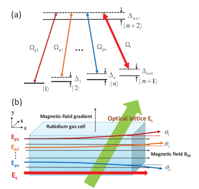
Figure 1: (Color online). (a): Atomic levels and excitation scheme. All quantities have been defined in the text. (b): A possible arrangement of experiment for observing the SG effect, where a SG gradient magnetic field $\textbf{B}_{\rm SG}(y)=\hat{\textbf{z}}(B_{0}+B_{1}y)$ is applied to the system. $\theta_{1},\theta_{2},\ldots,\theta_{n}$ are deflection angles of $n$ probe fields, respectively. The (green) thick arrow denotes the far-detuned optical lattice field $\textbf{E}_{\rm L}(x,t)=\hat{\textbf{y}}E_{0}\cos(x/R_{\perp})\cos(\omega_{\rm L}t)$ used to stabilize LBs. $\hat{\textbf{y}}$ and $\hat{\textbf{z}}$ are unit vectors along $y$ and $z$ directions, respectively. The probe and control fields are co-propagating laser beams to avoid Doppler shifts.

We assume that initially the atomic population is prepared in the ground states $|1\rangle$, $|2\rangle$,$\ldots$,$|n\rangle$, and cooled to a ultracold temperature in order to eliminate Doppler broadening and collisions. Fig. 1(b) is a possible arrangement of experimental apparatus. The aim of the co-propagating configuration of probe and control fields is also to avoid Doppler shifts.

We further assume a static SG gradient magnetic field

$$\textbf{B}_{\rm SG}(y)=\hat{\textbf{z}}B(y)=\hat{\textbf{z}}(B_{0}+B_{1}y)$$ (1)

is applied to the medium with $B_{1}\ll B_{0}$. Here $B_{0}$ contributes to a Zeeman level shift $\Delta E_{j,\textrm{Zeeman}}=\mu_{B}g_{F}^{j}m_{F}^{j}B_{0}$ for level $E_{j}$; $\mu_{B}$, $g_{F}^{j}$ and $m_{F}^{j}$ are Bohr magneton, gyromagnetic factor, and magnetic quantum number of the level $|j\rangle$, respectively; $B_{1}$ is the transverse gradient of the SG magnetic field, which will lead to SG deflection of the probe fields.

Additionally, we assume a small, far-detuned optical lattice field

$$\textbf{E}_{\rm L}(x,t)=\hat{\textbf{y}}E_{0}\cos(x/R_{\perp})\cos(\omega_{\rm L}t)$$ (2)

is also applied into the system, where $E_{0}$ , $R_{\perp}$ , and $\omega_{\rm L}$ are field amplitude, beam radius, and angular frequency, respectively note10 . Because of the existence of $\textbf{E}_{\rm L}(x,t)$, Stark level shift $\Delta E_{j,\textrm{Stark}}=-\alpha_{j}\langle E_{\rm L}^{2}(x,t)\rangle_{t}/2=-\alpha_{j}E_{\rm L}^{2}(x)/2$ occurs. Here $\alpha_{j}$ is the scalar polarizability of the level $|j\rangle$, $\langle Q(x,t)\rangle_{t}$ represents the time average in an oscillation cycle for the quantity $Q(x,t)$, and therefore we have $E_{\rm L}(x)=(E_{0}/\sqrt{2})\cos(x/R_{\perp})$. The aim of introducing the far-detuned optical field is to stabilize the LBs Hang ; Salerno .

Under electric-dipole and rotation wave approximations, the Hamiltonian of the atomic system in interaction picture is given by

$$\hat{H}_{\textrm{int}}= -\sum_{j=1}^{n+2}\hbar\Delta_{j}|j\rangle\langle j|-\hbar\left[\Omega_{p1}|n+2\rangle\langle 1|+\Omega_{p2}|n+2\rangle\langle 2|+\ldots+\Omega_{pn}|n+2\rangle\langle n|\right.$$ (3)

$$+\left.\Omega_{c}|n+2\rangle\langle n+1|+\textrm{H.c.}\right].$$

Here $\Omega_{pj}=({\textbf{e}}_{pj}\cdot{\textbf{p}}_{j,n+2}){\cal E}_{pj}/\hbar$ and $\Omega_{c}=({\textbf{e}}_{c}\cdot{\textbf{p}}_{n+1,n+2}){\cal E}_{c}/\hbar$ are Rabi frequencies of the $j$th probe and control fields, respectively, with ${\textbf{p}}_{jl}$ being the electric-dipole matrix element related to the states $|j\rangle$ and $|l\rangle$. The control field is so strong that it can be considered to be undepleted during the propagation of probe fields.

The equation of motion for the density matrix elements in interaction picture reads boyd

$$\frac{\partial\sigma}{\partial t}=-\frac{i}{\hbar}[H_{\rm int},\sigma]-\Gamma(\sigma),$$ (4)

where $\Gamma(\sigma)$ is a relaxation matrix denoting spontaneous emission and dephasing. The explicit form of Eq. (4) for $n=3$ is given in Appendix A.

The equation of motion for probe-field Rabi frequency $\Omega_{pj}$ can be derived by the Maxwell equation under slowly varying envelope approximation, given by Hua

$$i\left(\frac{\partial}{\partial z}+\frac{1}{c}\frac{\partial}{\partial t}\right)\Omega_{pj}+\frac{c}{2\omega_{pj}}\left(\frac{\partial^{2}}{\partial x^{2}}+\frac{\partial^{2}}{\partial y^{2}}\right)\Omega_{pj}+\kappa_{j,n+2}\sigma_{n+2,j}=0,$$ (5)

where $\kappa_{j,n+2}={\cal N}_{a}\omega_{pj}|\textbf{p}_{j,n+2}\cdot\textbf{e}_{pj}|^{2}/(2\epsilon_{0}c\hbar)$ $(j=1,2,\ldots,n)$, with ${\cal N}_{a}$ being the atomic concentration.

III Nonlinear envelope equations and light bullet solutions

III.1 Nonlinear envelope equations

One of our main aim is to get a stable propagation of all probe fields. On the one hand, the probe fields may suffer serious distortion due to the dispersion and diffraction of the system. On the other hand, EIT may result in a giant enhancement of Kerr effect. It is natural to use the enhanced Kerr effect to balance the dispersion and diffraction for obtaining solitonlike pulses that are shape-preserved during propagation.

To this end, we use the method of multiple scales Hua to derive nonlinear envelop equations of the probe fields. For simplicity, we consider the case of $n=3$ (The case for general $n$ will be taken into account in Sec. V). Taking the asymptotic expansion $\sigma_{ml}=\sum_{\alpha=0}^{\infty}\epsilon^{\alpha}\sigma_{ml}^{(\alpha)}$ ($m,\,l$=1-5), $\Omega_{pj}=\sum_{\alpha=1}^{\infty}\epsilon^{\alpha}\Omega_{pj}^{(\alpha)}$. Here $\sigma_{jj}^{(0)}$ is the population distribution prepared in the state $|j\rangle$ initially, which is assumed as $1/3$ ($j=1,2,3$) for simplicity; $\epsilon$ is a dimensionless small parameter characterizing the typical amplitude of the probe fields. All quantities on the right hand side of the expansions are considered as functions of the multi-scale variables $x_{1}=\epsilon x$, $y_{1}=\epsilon y$, $z_{\alpha}=\epsilon^{\alpha}z$ and $t_{\alpha}=\epsilon^{\alpha}t$ ($\alpha=0,2$). The SG gradient magnetic field and the far-detuned optical lattice field are assumed to be $B_{\rm SG}(y_{1})=B_{0}+\epsilon^{2}B_{1}y_{1}$ and $E_{\rm L}(x_{1})=\epsilon(E_{0}/\sqrt{2})\cos(x_{1}/R_{\perp})$. Thus, $\Delta_{j}$ can be expanded as $\Delta_{j}=\Delta_{j}^{(0)}+\epsilon^{2}\Delta_{j}^{(2)}$, where $\Delta_{2}^{(0)}=\omega_{p1}-\omega_{p2}-\omega_{21}-\mu_{21}B_{0}$, $\Delta_{3}^{(0)}=\omega_{p1}-\omega_{c}-\omega_{31}-\mu_{31}B_{0}$, $\Delta_{4}^{(0)}=\omega_{p1}-\omega_{41}-\mu_{41}B_{0}$, $\Delta_{5}^{(0)}=\omega_{p1}+\omega_{p2}-\omega_{c}-\omega_{51}-\mu_{51}B_{0}$, $\Delta_{2}^{(2)}=-\mu_{21}B_{1}y_{1}+\alpha_{21}E_{0}^{2}\cos^{2}(x_{1}/R_{\perp})/4$, $\Delta_{3}^{(2)}=-\mu_{31}B_{1}y_{1}+\alpha_{31}E_{0}^{2}\cos^{2}(x_{1}/R_{\perp})/4$, $\Delta_{4}^{(2)}=-\mu_{41}B_{1}y_{1}+\alpha_{41}E_{0}^{2}\cos^{2}(x_{1}/R_{\perp})/4$, and $\Delta_{5}^{(2)}=-\mu_{51}B_{1}y_{1}+\alpha_{51}E_{0}^{2}\cos^{2}(x_{1}/R_{\perp})/4$. Hence we have the form $d_{jl}=d_{jl}^{(0)}+\epsilon^{2}d_{jl}^{(2)}$, with $d_{jl}^{(0)}=\Delta_{j}^{(0)}-\Delta_{l}^{(0)}+i\gamma_{jl}$ and $d_{jl}^{(2)}=\Delta_{j}^{(2)}-\Delta_{l}^{(2)}$ [$\equiv-\mu_{jl}B_{1}y_{1}+\alpha_{jl}E_{0}^{2}\cos^{2}(x_{1}/R_{\perp})/4$].

At $\alpha=1$ order, we obtain the solution in linear level

$$\Omega_{pj}^{(1)}=F_{j}e^{i\theta_{j}},$$ (6a)

$$\sigma_{4j}^{(1)}=-\frac{\Omega_{c}^{\ast}\sigma_{jj}^{(0)}}{D_{j}}F_{j}e^{i\theta_{j}},$$ (6b)

$$\sigma_{5j}^{(1)}=\frac{(\omega+d_{4j}^{(0)})\sigma_{jj}^{(0)}}{D_{j}}F_{j}e^{i\theta_{j}}$$ (6c)

($j=1,\,2,\,3$). Here $D_{j}=|\Omega_{c}|^{2}-(\omega+d_{4j}^{(0)})(\omega+d_{5j}^{(0)})$, $\theta_{j}=K_{j}(\omega)z_{0}-\omega t_{0}$, with $F_{j}$ being envelope functions depending on slow variables $x_{1}$, $y_{1}$, $z_{2}$ and $t_{2}$ and $K_{j}(\omega)$ being the linear dispersion relations given by

$$K_{j}(\omega)=\frac{\omega}{c}+\frac{\kappa_{j5}\sigma_{jj}^{(0)}(\omega+d_{4j}^{(0)})}{D_{j}}.$$ (7)

In most cases $K_{j}(\omega)$ can be Taylor expanded around $\omega_{pj}$ (which corresponds to $\omega=0$) note1 , i.e. $K_{j}(\omega)=K_{j0}+K_{j1}\omega+\frac{1}{2}K_{j2}\omega^{2}+\cdots$, with $K_{jl}=[\partial^{l}K_{j}(\omega)/\partial\omega^{l}]|_{\omega=0}$ ($l=0$, 1, 2, $\cdots$). The coefficients $K_{jl}$ have rather clear physical interpretation, i.e. $K_{j0}={\rm Re}(K_{j0})+i{\rm Im}(K_{j0})$ gives the phase shift per unit length and absorption coefficient; $K_{j1}$ determines the group velocity given by $K_{j1}=1/V_{\textrm{g}j}=1/c+\kappa_{j5}\sigma_{jj}^{(0)}(|\Omega_{c}|^{2}+(\omega+d_{4j}^{(0)})^{2})/D_{j}^{2}$; and $K_{j2}=2\kappa_{j5}\sigma_{jj}^{(0)}(|\Omega_{c}|^{2}(3\omega+2d_{4j}^{(0)}+d_{5j}^{(0)})+(\omega+d_{4j}^{(0)})^{3})/D_{j}^{3}$ represent the group velocity dispersion which resulting in spreading and attenuation of the probe pulses.

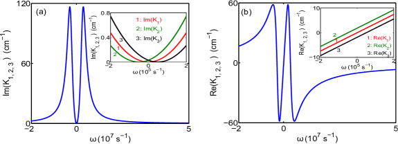
Figure 2: (Color online) Linear dispersion relations of the three probe fields. (a) $\textrm{Im}(K_{j})$ and (b) $\textrm{Re}(K_{j})$ ($j=1,2,3$) as functions of $\omega$. Each (blue) solid curve consists in fact of three curves, which can not be resolved since they nearly coincide each other due to the symmetry of the system. The inset in both panels show the absorption and dispersion curves near $\omega=0$. The curves 1, 2, 3 in the inset of panel (a) (panel (b)) are for Im$(K_{1})$, Im$(K_{2})$, Im$(K_{3})$ (Re$(K_{1})$, Re$(K_{2})$, Re$(K_{3})$), respectively. The parameters used for plotting the figure have been given in the text.

From Eq. (7) we see that the linear dispersion relation of the system has three branches. Fig. 2(a) and Fig. 2(b) show the absorption $\textrm{Im}(K_{j})$ and dispersion $\textrm{Re}(K_{j})$ $(j=1,\,2,\,3)$ of the three probe fields as functions of $\omega$, respectively. The parameters are chosen from a laser-cooled ⁸⁷Rb atomic gas with D₁ line transitions $5^{2}S_{1/2}\rightarrow 5^{2}P_{1/2}$ with atomic states assigned as $|1\rangle=|5^{2}S_{1/2},F=2,m_{F}=2\rangle$, $|2\rangle=|5^{2}S_{1/2},F=1,m_{F}=0\rangle$, $|3\rangle=|5^{2}S_{1/2},F=1,m_{F}=1\rangle$, $|4\rangle=|5^{2}S_{1/2},F=2,m_{F}=1\rangle$, and $|5\rangle=|5^{2}P_{1/2},F=2,m_{F}=1\rangle$ Steck . The decay rates are $\gamma_{41}\approx\gamma_{42}\approx\gamma_{43}=1$ kHz, and $\Gamma_{5}=5.75$ MHz. The other parameters are taken as $\kappa_{15}\approx\kappa_{25}\approx\kappa_{35}=1.0\times 10^{9}$ cm${}^{-1}\cdot$ s^-1, $\Delta_{2}=-5.0\times 10^{4}$ s^-1, $\Delta_{3}=5.0\times 10^{4}$ s^-1, $\Delta_{4}=\Delta_{5}=0$ s^-1, and $\Omega_{c}=3\times 10^{6}$ s^-1. We see that transparency windows are opened in the absorption curves Im$(K_{j})$ near $\omega=0$ ($j=1,2,3$), a typical character of EIT contributed by the control field-induced quantum interference effect. In fact, in linear regime the excitation scheme for $n=3$ (i.e. 4-pod configuration) consists of three independent $\Lambda$-type three-level systems and hence possesses three dark states, each of them displays EIT character. Note that the (blue) solid curve in both panels is a overlapping of three curves, which can not be resolved since they nearly coincide each other due to the symmetry of the system. The advantage of such symmetry is very useful for obtaining matching group velocities of different probe fields (i.e. ${\rm Re}(K_{11})\approx{\rm Re}(K_{21})\approx{\rm Re}(K_{31})$; Fig. 2(b)), which is very essential to obtain significant SG deflection of the probe fields.

At $\alpha=2$ order, we obtain solvability conditions $i[\partial F_{j}/\partial z_{1}+(\partial K_{j}/\partial\omega)\partial F_{j}/\partial t_{1}]=0$ ($j=1,\,2,\,3$), which indicate that the envelope function $F_{j}$ travels with complex group velocity $V_{{\rm g}j}\equiv(\partial K_{j}/\partial\omega)^{-1}$. Explicit expressions of the solution at this order have been presented in Appendix B.

At $\alpha=3$ order, the giant enhancement of Kerr effect of the system generated by EIT plays an important role. We obtain the coupled NLS equations governing the evolution of $F_{j}$:

$$i\left(\frac{\partial}{\partial z_{2}}+\frac{1}{V_{\textrm{g}j}}\frac{\partial}{\partial t_{2}}\right)F_{j}+\frac{c}{2\omega_{pj}}\left(\frac{\partial^{2}}{\partial x_{1}^{2}}+\frac{\partial^{2}}{\partial y_{1}^{2}}\right)F_{j}$$

$$-\sum_{l=1}^{3}W_{jl}|F_{l}|^{2}F_{j}e^{-2\bar{a}_{l}z_{2}}+[M_{j}B_{1}y_{1}+N_{j}E_{0}^{2}\cos^{2}(x_{1}/R_{\perp})]F_{j}=0,$$ (8)

($j=1,\,2,\,3$). Here $\bar{a}_{l}=\epsilon^{-2}\textrm{Im}(K_{l0})$; $W_{jl}$ result from the Kerr nonlinearity, which contribute to self-phase modulation (when $j=l$) and cross-phase modulation (when $j\neq l$), with explicit expressions given in Appendix C; $M_{j}$ and $N_{j}$ have the form

$$M_{j}=-\kappa_{j5}\frac{(\omega+d_{4j}^{(0)})^{2}\mu_{5j}+|\Omega_{c}|^{2}\mu_{4j}}{3D_{j}^{2}},$$ (9a)

$$N_{j}=\kappa_{j5}\frac{(\omega+d_{4j}^{(0)})^{2}\alpha_{5j}+|\Omega_{c}|^{2}\alpha_{4j}}{12D_{j}^{2}},$$ (9b)

characterizing the contributions of the SG gradient magnetic field and far-detunned optical lattice field, respectively.

III.2 Light bullet solutions

For convenience, we introduce the dimensionless variables $s=z/L_{\textrm{Diff}}$, $\tau=t/\tau_{0}$, $v_{\textrm{g}j}=V_{\textrm{g}j}\tau_{0}/L_{\textrm{Diff}}$, and $u_{j}=(\Omega_{pj}/U_{0})\exp[-i\textrm{Re}(K_{j0})z]$. Here $L_{\textrm{Diff}}=\omega_{p}R_{\perp}^{2}/c$, $\tau_{0}$, and $U_{0}$ are typical diffraction length, probe-field pulse duration, and half Rabi frequency, respectively. Then Eq. (III.1) can be written into the dimensionless form

$$\left[i\left(\frac{\partial}{\partial s}+\frac{1}{v_{\textrm{g}j}}\frac{\partial}{\partial\tau}\right)+\frac{1}{2}\left(\frac{\partial^{2}}{\partial\xi^{2}}+\frac{\partial^{2}}{\partial\eta^{2}}\right)\right]u_{j}-\sum_{l=1}^{3}\textrm{g}_{jl}|u_{l}|^{2}u_{j}+V_{j}(\xi,\eta)u_{j}=-iA_{j}u_{j},$$ (10)

where $\textrm{g}_{jl}=W_{jl}/|W_{12}|$ characterize nonlinear effect; and $A_{j}=\textrm{Im}(K_{j0})L_{\textrm{Diff}}$ ($j=$1, 2, 3) are absorption coefficients. The potential functions in Eq. (10) read

$$V_{j}(\xi,\eta)=\mathcal{M}_{j}\eta+\mathcal{N}_{j}\cos^{2}(\xi),$$ (11)

with $\mathcal{M}_{j}=L_{\textrm{Diff}}M_{j}R_{\perp}B_{1}$ and $\mathcal{N}_{j}=L_{\textrm{Diff}}N_{j}E_{0}^{2}$ ($j=1,\,2,\,3$). Note that in the derivation of Eq. (10) we have assumed $\tau_{0}$ is large so that group-velocity dispersion term (i.e., the term proportional to $\partial^{2}u_{j}/\partial\tau^{2}$) can be neglected, which can be easily realized experimentally. Furthermore, the absorption can also be negligible by choosing suitable system parameters under the condition of EIT. In fact, when we take $\tau_{0}=9.0\times 10^{-7}$ s, $U_{0}=3.38\times 10^{6}\,$s^-1, $\Delta_{2}=1.2\times 10^{4}\,$s^-1, $\Delta_{3}=1.5\times 10^{4}\,$s^-1, $\Delta_{4}=2.0\times 10^{5}\,$s^-1, $\Delta_{5}=9.0\times 10^{6}\,$s^-1, $\Omega_{c}=2.0\times 10^{7}$s^-1, and $R_{\perp}=36\,\mu$m with other parameters the same as in Fig. 2, we obtain the typical diffraction length $L_{\textrm{Diff}}=1.0$ cm, which is approximately equal to the typical nonlinearity length $L_{\textrm{N}}[\equiv 1/(U_{0}^{2}|W_{12}|)]$. However, the typical linear absorption length $L_{\textrm{A}\,j}=1/\textrm{Im}(K_{j0})$ is around $924.0$ cm and typical second-order dispersion length $L_{\textrm{Disp}\,j}=\tau_{0}^{2}/{\textrm{Re}}(K_{j2})$ ($j=1,2,3$) is $20.5$ cm, both of them are much larger than $L_{\textrm{Diff}}$ and $L_{\textrm{N}}$. Base on the results, we thus have the ratio coefficients $d_{j}=L_{\textrm{Diff}}/L_{\textrm{Disp}j}\approx 0.0495$, and $A_{j}=L_{\textrm{Diff}}/L_{\textrm{A}\,j}\approx 0.0011$, which describe the significance of the various characteristic interaction lengths relative to the diffraction effect. Therefore we can safely neglect the corresponding terms because they are much smaller than 1.

With the above parameters we obtain group velocities of three probe field envelopes (i.e. $\tilde{V}_{\textrm{g}j}={\rm Re}(\partial K_{j}/\partial\omega)^{-1}$ )

$$\tilde{V}_{\textrm{g}1}=3.964\times 10^{-5}\,c,$$ (12)

$$\tilde{V}_{\textrm{g}2}=3.966\times 10^{-5}\,c,$$ (13)

$$\tilde{V}_{\textrm{g}3}=3.967\times 10^{-5}\,c.$$ (14)

We see that three group velocities of probe field envelopes are very small comparing with $c$ ($c$ is light speed in vacuum), and nearly matched each other. The ultraslow and matched group velocities are essential to obtain significant SG deflection of the probe fields, as will be shown below.

We now seek approximated analytical solutions of the Eq. (10) with the form guo $u_{j}(\rho_{j},\tau,\xi,\eta)=f_{j}(\rho_{j})v_{j}(\tau,\xi,\eta)$, where $f_{j}(\rho_{j})$ are normalized Gaussian functions, that is, $f_{j}=[1/(\rho_{0}\sqrt{\pi})]^{1/2}\exp[-\rho_{j}^{2}/(2\rho_{0}^{2})]$ with $\rho_{j}=s-v_{gj}\tau$ and $\rho_{0}$ a constant. Integrating out the variable $\rho_{j}$, Eq. (10) becomes

$$\left[\frac{i}{v_{\textrm{g}j}}\frac{\partial}{\partial\tau}+\frac{1}{2}\left(\frac{\partial^{2}}{\partial\xi^{2}}+\frac{\partial^{2}}{\partial\eta^{2}}\right)\right]v_{j}-\frac{1}{\sqrt{2\pi}\rho_{0}}\sum_{l=1}^{3}\textrm{g}_{jl}|v_{l}|^{2}v_{j}+V_{j}(\xi,\eta)v_{j}=0.$$ (15)

To obtain the LB solutions of Eq. (15), we consider several reasonable approximations: (i)In the presence of the SG gradient magnetic field, the three probe-field envelopes will separate each other after propagating some distance. In such situation, the interaction between different envelopes becomes weak and hence the cross-phase-modulation terms can be neglected; (ii)The potential wells of the optical lattice are assumed to be deep enough, so that the probe-field envelopes are almost trapped in the wells in $x$ direction. Hence $V_{j}(\xi,\eta)$ given in Eq. (11) can be approximated by $\mathcal{M}_{j}\eta+\mathcal{N}_{j}-\mathcal{N}_{j}\xi^{2}$. Thus Eq. (15) can be approximated as

$$\left[\frac{i}{v_{\textrm{g}j}}\frac{\partial}{\partial\tau}+\frac{1}{2}\left(\frac{\partial^{2}}{\partial\xi^{2}}+\frac{\partial^{2}}{\partial\eta^{2}}\right)\right]v_{j}-\frac{1}{\sqrt{2\pi}\rho_{0}}\textrm{g}_{jj}|v_{j}|^{2}v_{j}+(\mathcal{M}_{j}\eta+\mathcal{N}_{j}-\mathcal{N}_{j}\xi^{2})v_{j}=0.$$ (16)

Assuming $v_{j}({\tau,\xi,\eta})=w_{j}(\tau,\eta)\phi_{j}(\xi)\exp(i\mathcal{N}_{j}v_{\textrm{g}j}\tau)$, where $\phi_{j}(\xi)$ is a normalized ground state solution satisfying the eigenvalue problem $(\partial^{2}/\partial\xi^{2}-2\mathcal{N}_{j}\xi^{2})\phi_{j}=2E_{\xi}\phi_{j}$ with $E_{\xi}=-\sqrt{\mathcal{N}_{j}/2}$, and integrating over the variable $\xi$, one obtains

$$\left(\frac{i}{v_{\textrm{g}j}}\frac{\partial}{\partial\tau}+\frac{1}{2}\frac{\partial^{2}}{\partial\eta^{2}}\right)w_{j}-\frac{\mathcal{N}_{j}^{1/4}}{2^{3/4}\pi\rho_{0}}\textrm{g}_{jj}|w_{j}|^{2}w_{j}+\left(\mathcal{M}_{j}\eta-\sqrt{\frac{\mathcal{N}_{j}}{2}}\right)w_{j}=0.$$ (17)

Eq. (17) is a (1+1)-dimensional NLS equation with a linear potential, which admits the exact single-soliton solutions Yan

$$w_{j}=\mathcal{A}_{j}e^{i\varphi_{j}}{\textrm{sech}}\Theta_{j},$$ (18)

where $\mathcal{A}_{j}=(2^{5/4}\mathcal{N}_{j}^{1/4}\pi\rho_{0}/|{\textrm{g}_{jj}}|)^{1/2}$, $\varphi_{j}=\mathcal{M}_{j}v_{{\textrm{g}}j}\tau(\eta-\mathcal{M}_{j}v_{{\textrm{g}}j}^{2}\tau^{2}/6)$, and $\Theta_{j}=(2\mathcal{N}_{j})^{1/4}(\eta-\mathcal{M}_{j}v_{{\textrm{g}}j}^{2}\tau^{2}/2)$. Finally, we obtain the solution of Eq. (15)

$$u_{j}=\mathcal{A}_{j}[1/(\rho_{0}\sqrt{\pi})]^{1/2}(\sqrt{2\mathcal{N}_{j}}/\pi)^{1/4}e^{i\varphi_{j}}e^{-(s-v_{{\textrm{g}}j}\tau)^{2}/(2\rho_{0}^{2})}e^{-\sqrt{\mathcal{N}_{j}}\xi^{2}/\sqrt{2}}{\textrm{sech}}\Theta_{j},$$ (19)

which is a nonlinear solution localized in three space and one time dimensions, i.e. the (3+1)-dimensional LB solution of the system.

IV Stern-Gerlach deflection of 3-component ultraslow light bullets

When returning to original variables, the LB solution (19) has the form

$$\Omega_{pj}= U_{0}\mathcal{A}_{j}\left(\frac{1}{\rho_{0}\sqrt{\pi}}\right)^{1/2}\left(\frac{\sqrt{2\mathcal{N}_{j}}}{\pi}\right)^{1/4}e^{i\varphi_{j}}e^{-\sqrt{\mathcal{N}_{j}}x^{2}/(\sqrt{2}R_{\perp}^{2})}e^{-(z-\tilde{V}_{gj}t)^{2}/(2L_{\rm Diff}^{2}\rho_{0}^{2})}$$ (20)

$$\times{\rm sech}\left\{\frac{(2\mathcal{N}_{j})^{1/4}}{R_{\perp}}\left(y-\frac{\mathcal{M}_{j}R_{\perp}\tilde{V}_{gj}^{2}}{2L_{\rm Diff}^{2}}t^{2}\right)\right\}.$$

We see that the LB travels in $z$ direction with ultraslow group velocity $\tilde{V}_{gj}$. In addition, it has an acceleration $\mathcal{M}_{j}R_{\perp}\tilde{V}_{gj}^{2}/L_{\rm Diff}^{2}$ in $y$ direction, which results in the SG deflection. Note that $\mathcal{M}_{j}$ is proportional to the parameter $B_{1}$, i.e. the deflection comes from the SG gradient magnetic field given by Eq. (1).

Shown in Fig. 3

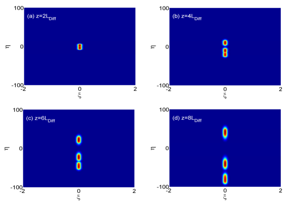
Figure 3: (Color online) The SG deflection spectrum of the 3-component ultraslow LB. (a), (b), (c) and (d) are deflections of the LB when propagating to $z=2L_{\rm Diff}$, $z=4L_{\rm Diff}$, $z=6L_{\rm Diff}$, and $z=8L_{\rm Diff}$, respectively. The bright spots from top to bottom are distributions of $|\mathcal{E}_{p1}|^{2}$, $|\mathcal{E}_{p2}|^{2}$, and $|\mathcal{E}_{p3}|^{2}$ in $x$-$y$ plane, respectively.

is the result of the SG deflection spectrum of the 3-component LB by numerically simulating Eq. (16) with $B_{1}\neq 0$. Panels (a), (b), (c), and (d) give the light intensity of the LB when propagating respectively to $z=2L_{\rm Diff}$, $z=4L_{\rm Diff}$, $z=6L_{\rm Diff}$, and $z=8L_{\rm Diff}$ for $B_{1}=1.2\,$mG/mm and $E_{0}=5.0\times 10^{4}\,$V/m. The bright spots from top to bottom in each panel are distributions of $|\mathcal{E}_{p1}|^{2}$, $|\mathcal{E}_{p2}|^{2}$, and $|\mathcal{E}_{p3}|^{2}$ in $x$-$y$ plane, respectively. Through the information of Fig. 3, we can see that an obvious deflection track of LBs occurs due to the SG gradient magnetic field existing. The phenomenon is similar to the SG deflection for atoms.

We now determine the SG deflection angles of each LB components. From the solution (20) we get the propagating velocity of the $j$th LB component at time $t$

$${\bf V}_{j}=\left(0,\frac{\mathcal{M}_{j}\tilde{V}_{{\rm g}j}^{2}R_{\perp}}{L_{\textrm{Diff}}^{2}}t,\tilde{V}_{{\rm g}j}\right).$$ (21)

Assume the medium length in the $z$ direction is $L$. The running time in $z$ direction is thus $L/\tilde{V}_{{\rm g}j}$. At the exit of the medium the velocity of the $j$th LB component will be ${\bf V}_{j}=(0,V_{yj},\tilde{V}_{{\rm g}j})$ with $V_{yj}=\mathcal{M}_{j}\tilde{V}_{{\rm g}j}R_{\perp}L/L_{\textrm{Diff}}^{2}$. As a result, we have the deflection angle after passing through the medium

$$\theta_{j}=\frac{V_{yj}}{\tilde{V}_{{\textrm{g}}j}}=\frac{L}{\tilde{V}_{{\textrm{g}}j}}\frac{\mu_{\textrm{sol}\,j}}{p_{j}}r^{2}B_{1},$$ (22)

where $r=R_{\perp}/L_{\textrm{Diff}}$, $p_{j}=\hbar k_{pj}$ is photon momentum, and $\mu_{\textrm{sol}\,j}=L_{\textrm{Diff}}M_{j}\tilde{V}_{{\textrm{g}}j}\hbar k_{pj}$ is effective magnetic moment note2 . With the data given in Fig. 3 we obtain $\mu_{\textrm{sol}\,1,\,2}=\pm 3.70\times 10^{-19}$ J/T and $\mu_{\textrm{sol}\,3}=-7.41\times 10^{-19}$ J/T. The center position of the $j$th probe envelope at the exit of the medium reads

$$(x_{j},y_{j},z_{j})=\left(0,\frac{\mathcal{M}_{j}L^{2}R_{\perp}}{2L_{\textrm{Diff}}^{2}},L\right).$$ (23)

From the formula (22) we see that the deflection angle $\theta_{j}$ is inversely proportional to $\tilde{V}_{{\rm g}j}$. So the ultraslow group velocity $\tilde{V}_{{\rm g}j}$ induced by the EIT effect can result in large SG deflection angles of the LB.

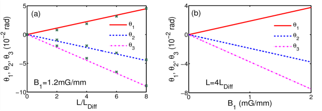
Figure 4: (Color online) (a): Deflection angles of the LB components as functions of medium length $L$ for magnetic field gradient $B_{1}=1.2\,$mG/mm. The solid, dashed and dashed-dotted lines denote deflection angles $\theta_{1}$, $\theta_{2}$ and $\theta_{3}$, respectively. Points labeled by $``\times"$ are center positions of the LBs components obtained numerically. (b): Deflection angles of the LB components as functions of $B_{1}$ for $L=4L_{\textrm{Diff}}$. The results of $\theta_{1}$, $\theta_{2}$ and $\theta_{3}$ are respectively labeled by solid, dashed and dashed-dotted lines.

Shown in Fig. 4(a) are deflection angles of the LB components as functions of medium length $L$ for magnetic field gradient $B_{1}=1.2\,$mG/mm. The solid, dashed and dashed-dotted lines denote respectively deflection angles $\theta_{1}$, $\theta_{2}$ and $\theta_{3}$ obtained by using the formula (22) for $\tilde{V}_{\rm g1}\simeq\tilde{V}_{\rm g2}\simeq\tilde{V}_{\rm g3}\approx 4.0\times 10^{-5}c$. Points labeled by $``\times"$ are numerical results of the center position of LBs components obtained in Fig. 3. From the figure, we obtain $(\theta_{1},\,\theta_{2},\,\theta_{3})=(2.25,\,-2.24,\,-4.49)\times 10^{-2}$ rad for $L=4L_{\textrm{Diff}}$, which is three orders of magnitude larger than that for linear polariton obtained in Weitz .

The SG effect of the LBs demonstrated above may show many intriguing applications. For instance, through measuring the deflection angles of LBs components, one can obtain the gradient magnetic field $B_{1}$. Fig. 4(b) shows the deflection angles as functions of $B_{1}$ for $L=4L_{\textrm{Diff}}$. The results of $\theta_{1}$, $\theta_{2}$ and $\theta_{3}$ are respectively labeled by solid, dashed and dashed-dotted lines. We see that the larger the magnetic field gradient, the larger the SG deflection angles. We expect that the significant SG deflection obtained here may have potential applications in optical magnetometery and quantum information processing, etc.

V SG effect of $n$-component ultraslow light bullets

We now investigate the SG deflection of multi-component ultraslow LBs in a $(n+2)$-level system via EIT. For the $(n+1)$-pod level configuration ($n>3$) shown in Fig. 1(a), the theoretical approach is a direct generation of that developed in last two sections. Using the weak nonlinear perturbation theory Hua , we can obtain the following coupled NLS equations

$$i\left(\frac{\partial}{\partial z_{2}}+\frac{1}{V_{\textrm{g}j}}\frac{\partial}{\partial t_{2}}\right)F_{j}+\frac{c}{2\omega_{pj}}\left(\frac{\partial^{2}}{\partial x_{1}^{2}}+\frac{\partial^{2}}{\partial y_{1}^{2}}\right)F_{j}$$

$$-\sum_{l=1}^{n}W_{jl}|F_{l}|^{2}e^{-2{\bar{a}}_{l}z_{2}}F_{j}+[M_{j}B_{1}y_{1}+N_{j}E_{0}^{2}\cos^{2}(x_{1}/R_{\perp})]F_{j}=0,$$ (24)

($j=1,2,\ldots,n$). Here $F_{j}$ is the envelope of the $j$th probe field; $W_{jl}$ are coefficients of self-phase (for $j=l$) and cross-phase (for $j\neq l$) modulations; $M_{j}$ ($N_{j}$) characterize the amplitude of the SG gradient magnetic field (the far-detuned optical lattice field). Explicit expressions of these coefficients are lengthy and omitted here.

A similar approach as in the last two sections can also be done. For SG deflection problem, what we want is the result in far-field approximation, i.e. the one for a larger propagation distance where different the LB components are separated away. Thus the cross-phase modulation terms in Eq. (V) can be neglected reasonably. By assuming a strong confinement from the far-detuned optical lattice potential, we can obtain an equation similar to (16), and LB solution with the same form of (20).

In this case, we also numerically simulate Eq. (16) with $B_{1}\neq 0$ to investigate the deflection of $n$-component LBs. Shown in Fig. 5 is the SG deflection spectrum of a $5$-component ultraslow LB. Panels (a), (b), (c) and (d) show the light intensity of the LB components when propagating to $z=2L_{\rm Diff}$, $z=4L_{\rm Diff}$, $z=6L_{\rm Diff}$, and $z=8L_{\rm Diff}$, respectively. We see that the LB is robust during propagation and its components separate away fast in $y$ direction. Such result can be taken as a satisfactory analog of general SG effect of atoms for angular-momentum quantum number $J>1/2$.

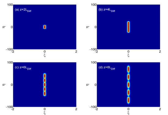
Figure 5: (Color online) The SG deflection spectrum of $5$-component ultraslow LB. (a), (b), (c) and (d) show the deflections of the LB components when propagating to $z=2L_{\rm Diff}$, $z=4L_{\rm Diff}$, $z=6L_{\rm Diff}$, and $z=8L_{\rm Diff}$, respectively.

VI Summary

We have suggested a scheme to exhibit a Stern-Gerlach effect of $n$-component ($n>2$) high-dimensional ultraslow optical solitons in a coherent atomic system with $(n+1)$-pod level configuration via EIT. Based on the MB equations, we have derived the coupled (3+1)-dimensional NLS equations governing the spatial-temporal evolution of the $n$ probe-field envelopes. We have demonstrated that under the EIT condition significant deflections of the $n$ components of the ultraslow LBs can be achieved by using a Stern-Gerlach gradient magnetic field. The stability of the ultraslow LBs can be realized by an optical lattice potential contributed from a far-detuned laser field. We expect that the results predicted here may have potential applications in the research fields of optical magnetometery, light information processing, and so on.

Appendix A Equations of motion of density matrix elements

The elements of density matrix for $n=3$ read

$$i\frac{\partial}{\partial t}\sigma_{11}-i\Gamma_{15}\sigma_{55}+\Omega_{p1}^{\ast}\sigma_{51}-\Omega_{p1}\sigma_{51}^{\ast}=0,$$ (25a)

$$i\frac{\partial}{\partial t}\sigma_{22}-i\Gamma_{25}\sigma_{55}+\Omega_{p2}^{\ast}\sigma_{52}-\Omega_{p2}\sigma_{52}^{\ast}=0,$$ (25b)

$$i\frac{\partial}{\partial t}\sigma_{33}-i\Gamma_{35}\sigma_{55}+\Omega_{p3}^{\ast}\sigma_{53}-\Omega_{p3}\sigma_{53}^{\ast}=0,$$ (25c)

$$i\frac{\partial}{\partial t}\sigma_{44}-i\Gamma_{45}\sigma_{55}+\Omega_{c}^{\ast}\sigma_{54}-\Omega_{c}\sigma_{54}^{\ast}=0,$$ (25d)

$$i(\frac{\partial}{\partial t}+\Gamma_{5})\sigma_{55}+\Omega_{p1}\sigma_{51}^{\ast}+\Omega_{p2}\sigma_{52}^{\ast}+\Omega_{p3}\sigma_{53}^{\ast}$$

$$+\Omega_{c}\sigma_{54}^{\ast}-\Omega_{p1}^{\ast}\sigma_{51}-\Omega_{p2}^{\ast}\sigma_{52}-\Omega_{p3}^{\ast}\sigma_{53}-\Omega_{c}^{\ast}\sigma_{54}=0,$$ (25e)

$$(i\frac{\partial}{\partial t}+d_{21})\sigma_{21}+\Omega_{p2}^{\ast}\sigma_{51}-\Omega_{p1}\sigma_{52}^{\ast}=0,$$ (25f)

$$(i\frac{\partial}{\partial t}+d_{31})\sigma_{31}+\Omega_{p3}^{\ast}\sigma_{51}-\Omega_{p1}\sigma_{53}^{\ast}=0,$$ (25g)

$$(i\frac{\partial}{\partial t}+d_{32})\sigma_{32}+\Omega_{p3}^{\ast}\sigma_{52}-\Omega_{p2}\sigma_{53}^{\ast}=0,$$ (25h)

$$(i\frac{\partial}{\partial t}+d_{41})\sigma_{41}+\Omega_{c}^{\ast}\sigma_{51}-\Omega_{p1}\sigma_{54}^{\ast}=0,$$ (25i)

$$(i\frac{\partial}{\partial t}+d_{42})\sigma_{42}+\Omega_{c}^{\ast}\sigma_{52}-\Omega_{p2}\sigma_{54}^{\ast}=0,$$ (25j)

$$(i\frac{\partial}{\partial t}+d_{43})\sigma_{43}+\Omega_{c}^{\ast}\sigma_{53}-\Omega_{p3}\sigma_{54}^{\ast}=0,$$ (25k)

$$(i\frac{\partial}{\partial t}+d_{51})\sigma_{51}+\Omega_{p1}(\sigma_{11}-\sigma_{55})+\Omega_{p2}\sigma_{21}+\Omega_{p3}\sigma_{31}+\Omega_{c}\sigma_{41}=0,$$ (25l)

$$(i\frac{\partial}{\partial t}+d_{52})\sigma_{52}+\Omega_{p2}(\sigma_{22}-\sigma_{55})+\Omega_{p1}\sigma_{21}^{\ast}+\Omega_{p3}\sigma_{32}+\Omega_{c}\sigma_{42}=0,$$ (25m)

$$(i\frac{\partial}{\partial t}+d_{53})\sigma_{53}+\Omega_{p3}(\sigma_{33}-\sigma_{55})+\Omega_{p1}\sigma_{31}^{\ast}+\Omega_{p2}\sigma_{32}^{\ast}+\Omega_{c}\sigma_{43}=0,$$ (25n)

$$(i\frac{\partial}{\partial t}+d_{54})\sigma_{54}+\Omega_{c}(\sigma_{44}-\sigma_{55})+\Omega_{p1}\sigma_{41}^{\ast}+\Omega_{p2}\sigma_{42}^{\ast}+\Omega_{p3}\sigma_{43}^{\ast}=0,$$ (25o)

with $d_{jl}=\Delta_{j}-\Delta_{l}+i\gamma_{jl}$. Here detunings are defined by $\Delta_{2}=\omega_{p1}-\omega_{p2}-\omega_{21}-\mu_{21}B(y)+\alpha_{21}E(x)^{2}/2$, $\Delta_{3}=\omega_{p1}-\omega_{p3}-\omega_{31}-\mu_{31}B(y)+\alpha_{31}E(x)^{2}/2$, $\Delta_{4}=\omega_{p1}-\omega_{c}-\omega_{41}-\mu_{41}B(y)+\alpha_{41}E(x)^{2}/2$, $\Delta_{5}=\omega_{p1}-\omega_{51}-\mu_{51}B(y)+\alpha_{51}E(x)^{2}/2$, with $\mu_{jl}=\mu_{B}(g_{F}^{j}m_{F}^{j}-g_{F}^{l}m_{F}^{l})/\hbar$, $\alpha_{jl}=(\alpha_{j}-\alpha_{l})/\hbar$, $\omega_{jl}=(E_{j}-E_{l})/\hbar$. Dephasing rates are $\gamma_{jl}=(\Gamma_{j}+\Gamma_{l})/2+\gamma_{jl}^{\rm col}$, with $\Gamma_{j}=\sum_{E_{i}<E_{j}}\Gamma_{ij}$ denoting the spontaneous emission rates of the state $|j\rangle$ and $\gamma_{jl}^{\rm col}$ denoting the dephasing rate reflecting the loss of phase coherence between $|j\rangle$ and $|l\rangle$, as might occur with elastic collisions.

Appendix B Explicit expressions of the second order solutions

The second-order solution for $n=3$ reads

$$\sigma_{21}^{(2)}=\frac{\Omega_{p1}^{(1)}\sigma_{52}^{\ast(1)}-\Omega_{p2}^{\ast(1)}\sigma_{51}^{(1)}}{\omega+d_{21}},$$ (26a)

$$\sigma_{31}^{(2)}=\frac{\Omega_{p1}^{(1)}\sigma_{53}^{\ast(1)}-\Omega_{p3}^{\ast(1)}\sigma_{51}^{(1)}}{\omega+d_{31}},$$ (26b)

$$\sigma_{32}^{(2)}=\frac{\Omega_{p2}^{(1)}\sigma_{53}^{\ast(1)}-\Omega_{p3}^{\ast(1)}\sigma_{52}^{(1)}}{\omega+d_{32}},$$ (26c)

$$\sigma_{4j}^{(2)}=\frac{1}{D_{j}}\left[(\omega+d_{5j})i\frac{\partial}{\partial t_{1}}\sigma_{4j}^{(1)}-\Omega_{c}^{\ast}i\frac{\partial}{\partial t_{1}}\sigma_{5j}^{(1)}\right],$$ (26d)

$$\sigma_{5j}^{(2)}=\frac{1}{D_{j}}\left[(\omega+d_{4j})i\frac{\partial}{\partial t_{1}}\sigma_{5j}^{(1)}-\Omega_{c}i\frac{\partial}{\partial t_{1}}\sigma_{4j}^{(1)}\right],$$ (26e)

$$\sigma_{54}^{(2)}=-\frac{\Omega_{p1}^{(1)}\sigma_{41}^{\ast(1)}+\Omega_{p2}^{(1)}\sigma_{42}^{\ast(1)}+\Omega_{p3}^{(1)}\sigma_{43}^{\ast(1)}}{\omega+d_{54}}$$ (26f)

($j=1,\,2,\,3$), where $\sigma_{41}^{(1)}$, $\sigma_{42}^{(1)}$, $\sigma_{43}^{(1)}$, $\sigma_{51}^{(1)}$, $\sigma_{52}^{(1)}$, and $\sigma_{53}^{(1)}$ are obtained at the first order approximation. $d_{21}=\Delta_{21}^{(0)}+i\gamma_{21}$, $d_{31}=\Delta_{31}^{(0)}+i\gamma_{31}$, $d_{32}=\Delta_{32}^{(0)}+i\gamma_{32}$, and $d_{54}=\Delta_{54}^{(0)}+i\gamma_{54}$. For simplicity, the superscript of $(0)$ in $d_{jl}^{(0)}$ has been omitted in Eq. (26).

Appendix C Explicit expressions of $W_{jl}$ in Eq. (III.1)

The Kerr coefficients $W_{jl}$ in Eq. (III.1) are given by

$$W_{jj}=-\frac{\kappa_{j5}|\Omega_{c}|^{2}}{3D_{j}^{2}(\omega+d_{54}^{\ast})},\,\,(j=1,\,2\,,3)$$ (27a)

$$W_{12}=-\frac{\kappa_{15}}{3D_{1}}\left[\frac{\omega+d_{41}}{\omega+d_{21}}\left(\frac{\omega+d_{42}^{\ast}}{D_{2}^{\ast}}-\frac{\omega+d_{41}}{D_{1}}\right)+\frac{|\Omega_{c}|^{2}}{D_{2}(\omega+d_{54}^{\ast})}\right],$$ (27b)

$$W_{13}=-\frac{\kappa_{15}}{3D_{1}}\left[\frac{\omega+d_{41}}{\omega+d_{31}}\left(\frac{\omega+d_{43}^{\ast}}{D_{3}^{\ast}}-\frac{\omega+d_{41}}{D_{1}}\right)+\frac{|\Omega_{c}|^{2}}{D_{3}(\omega+d_{54}^{\ast})}\right],$$ (27c)

$$W_{21}=-\frac{\kappa_{25}}{3D_{2}}\left[\frac{\omega+d_{42}}{\omega+d_{21}^{\ast}}\left(\frac{\omega+d_{42}}{D_{2}}-\frac{\omega+d_{41}^{\ast}}{D_{1}^{\ast}}\right)+\frac{|\Omega_{c}|^{2}}{D_{1}(\omega+d_{54}^{\ast})}\right],$$ (27d)

$$W_{23}=-\frac{\kappa_{25}}{3D_{2}}\left[\frac{\omega+d_{42}}{\omega+d_{32}}\left(\frac{\omega+d_{43}^{\ast}}{D_{3}^{\ast}}-\frac{\omega+d_{42}}{D_{2}}\right)+\frac{|\Omega_{c}|^{2}}{D_{3}(\omega+d_{54}^{\ast})}\right],$$ (27e)

$$W_{31}=-\frac{\kappa_{35}}{3D_{3}}\left[\frac{\omega+d_{43}}{\omega+d_{31}^{\ast}}\left(\frac{\omega+d_{43}}{D_{3}}-\frac{\omega+d_{41}^{\ast}}{D_{1}^{\ast}}\right)+\frac{|\Omega_{c}|^{2}}{D_{1}(\omega+d_{54}^{\ast})}\right],$$ (27f)

$$W_{32}=-\frac{\kappa_{35}}{3D_{3}}\left[\frac{\omega+d_{43}}{\omega+d_{32}^{\ast}}\left(\frac{\omega+d_{43}}{D_{3}}-\frac{\omega+d_{42}^{\ast}}{D_{2}^{\ast}}\right)+\frac{|\Omega_{c}|^{2}}{D_{2}(\omega+d_{54}^{\ast})}\right],$$ (27g)

where the superscript of $(0)$ in $d_{jl}^{(0)}$ has been omitted for simplicity in this equation.

References

• (1) Y. Silberberg, “Collapse of optical pulses,” Opt. Lett. 15, 1282-1284 (1990).
• (2) Y. S. Kivshar and G. P. Agrawal, Optical Solitons: From Fibers to Photonic Crystals (Academic, San Diego, 2003).
• (3) M. Fleischhauer, A. Imamoǧlu, and J. P. Marangos, “Electromagnetically induced transparency: optics in coherent media,” Rev. Mod. Phys. 77, 633-673 (2005).
• (4) H.-j. Li, Y.-p. Wu, and G. Huang, “Stable weak light ultraslow spatiotemporal solitons via atomic coherence,” Phys. Rev. A 84, 033816 (2011).
• (5) R. Harré, Great Scientific Experiments: 20 experiments that changed our view of the world (Phaidon, Oxford, 1981).
• (6) J. J. Sakurai, Modern Quantum Mechanics (revised edition) (Addison-Wesley, Boston, 1994).
• (7) M. A. Nielsen and I. L. Chang, Quantum Computation and Quantum Information (Cambridge, UK, 2000).
• (8) N. A. Kuebler, M. B. Robin, J. J. Yang, and A. Gedanken, “Fully resolved Zeeman pattern in the Stern-Gerlach deflection spectrum of O2 (${}^{3}\Sigma_{g}^{-}$, $K=1$),” Phys. Rev. A 38, 737-749 (1988).
• (9) A. Gedanken, N. A. Kuebler, M. B. Robin, and D. R. Herrick, “Stern-Gerlach deflection spectra of nitrogen oxide radicals,” J. Chem. Phys. 90, 3981-3993 (1989).
• (10) Y. Li, C. Bruder, and C. P. Sun, “Generalized Stern-Gerlach effect for chiral molecules,” Phys. Rev. Lett. 99, 130403 (2007).
• (11) W. D. Knight, R. Monot, E. R. Dietz, and A. R. George, “Stern-Gerlach deflection of metallic-cluster beams,” Phys. Rev. Lett. 40, 1324-1326 (1978).
• (12) S. Pokrant, “Evidence for adiabatic magnetization of cold DyN clusters,” Phys. Rev. A, 62, 051201(R) (2000).
• (13) X. Xu, S. Yin, R. Moro, and W. A. de Heer, “Magnetic moments and adiabatic magnetization of free cobalt clusters,” Phys. Rev. Lett., 95, 237209 (2005).
• (14) F. W. Payne, W. Jiang, J. W. Emmert, J. Deng, and L. A. Bloomfield, “Magnetic structure of free cobalt clusters studied with Stern-Gerlach deflection experiments,” Phys. Rev. B, 75, 094431 (2007).
• (15) S. Peredkov, M. Neeb, W. Eberhardt, J. Meyer, M. Tombers, H. Kampschulte, and G. Niedner-Schatteburg, “Spin and orbital magnetic moments of free nanoparticles,” Phys. Rev. Lett. 107, 233401 (2011).
• (16) L. Karpa and M. Weitz, “A Stern-Gerlach experiment for slow light,” Nat. Phys. 2, 332-335 (2006).
• (17) C. Hang and G. Huang, “Stern-Gerlach effect of weak-light ultraslow vector solitons,” Phys. Rev. A, 86, 043809 (2012).
• (18) Generaly, an atomic beam will split into $2J+1$ different beams when passing through a SG magnetic field. See, e.g., G. Herzberg, Atomic Spectra and Atomic Structure (Dover, New York, 1944).
• (19) The far-detuned optical field (2) will generates a magnetic field ${\bf B}_{m}(x,t)=\hat{\bf z}(E_{0}/c)\sin(x/R_{\perp})\sin(\omega_{L}t)$. In our model, we choose $\omega_{L}\sim 10^{13}$ Hz, which is far from any resonance in atoms. It is easy to show that the magnitude of the effective magnetic field resulted from ${\bf B}_{m}(x,t)$ is proportional to $E_{0}^{2}/(4c^{2}B_{0})$, which is around $6.94\times 10^{-4}$ Gauss when taking $E_{0}\sim 5\times 10^{4}$ V/m and $B_{0}=1.0\times 10^{3}$ Gauss. Because the second term of the SG magnetic field $|B_{1}y|\leq|B_{1}L_{y}|\sim 4.32\times 10^{-3}$ Gauss for $L_{y}\sim 100R_{\perp}$ ($L_{y}$ is the deflection distance in the $y$ direction used below), the magnetic field ${\bf B}_{m}$ generated by the far-detuned optical field (2) can be safely neglected for the SG deflection considered here.
• (20) B. B. Baizakov, B. A Malomed, and M. Salerno, “Multidimensional solitons in a low-dimensional periodic potential,” Phys. Rev. A 70, 053613 (2004).
• (21) R. W. Boyd, Nonlinear Optics (3rd edition) (Academic, Elsevier, 2008).
• (22) G. Huang, L. Deng, and M. G. Payne,“Dynamics of ultraslow optical solitons in a cold three-state atomic system,” Phys. Rev. E 72, 016617 (2005).
• (23) In the atomic medium, the frequency and wave number of the $j$th probe field are given by $\omega_{pj}+\omega$ and $k_{pj}+K_{j}(\omega)$, respectively. Thus $\omega=0$ corresponds to the center frequency of all probe fields.
• (24) D. A. Steck, Rubidium 87 D Line Data [http://steck.us/alkalidata/].
• (25) Y. Guo, L. Zhou, L.-M. Kuang, and C. P. Sun, “Magneto-optical Stern-Gerlach effect in an atomic ensemble,” Phys. Rev. A 78, 013833 (2008).
• (26) J. Yan, G. Zhou, and J. You, “Nonpropagating soliton and kink soliton in a mildly sloping channel,” Phys. Fluids A 4, 690-694 (1992).
• (27) Photons in vacuum have no magnetic momemt, and hence experience no force and have no trajectroy deflection when passing through an inhomogeneous magnetic field. However, photons may acquire effective magnetic moments in atomic media, thus experience a magnetic force and display the SG effect.