Cage–jump motion reveals universal dynamics and non–universal structural features in glass forming liquids

The sluggish and heterogeneous dynamics of glass forming liquids is frequently associated to the transient coexistence of two phases of particles, respectively with an high and low mobility. In the absence of a dynamical order parameter that acquires a transient bimodal shape, these phases are commonly identified empirically, which makes difficult investigating their relation with the structural properties of the system. Here we show that the distribution of single particle diffusivities can be accessed within a Continuous Time Random Walk description of the intermittent motion, and that this distribution acquires a transient bimodal shape in the deeply supercooled regime, thus allowing for a clear identification of the two coexisting phase. In a simple two-dimensional glass forming model, the dynamic phase coexistence is accompanied by a striking structural counterpart: the distribution of the crystalline-like order parameter becomes also bimodal on cooling, with increasing overlap between ordered and immobile particles. This simple structural signature is absent in other models, such as the three-dimesional Kob-Andersen Lennard-Jones mixture, where more sophisticated order parameter might be relevant. In this perspective, the identification of the two dynamical coexisting phases opens the way to deeper investigations of structure-dynamics correlations.

Keywords: Slow relaxation and glassy dynamics, Structural glasses (Theory), Dynamical heterogeneities (Theory).

1 Introduction

Probably the main paradox of structural glasses is the apparent mismatch between dynamics and structure: the dynamics dramatically slows down on cooling, as highlighted by the huge grow of the relaxation time. By contrast, the structure remains seemingly unchanged, insomuch as it is not possible to distinguish a glass from a simple liquids simply focussing on pair correlation functions, such as the structure factor or the radial distribution function^{1; 2; 3}. However, recent results suggested that structural fingerprints of glasses can be found in higher order geometrical motifs, known as locally preferred structures (LPS), or more sophisticated order parameter, such as the local configurational entropy⁴, or introducing an external perturbation, such as particle pinning^{5; 6} or static shear⁷.

A key to investigate the interplay between structure and dynamics arises from the observation of the temporary clustering of particles with similar mobility, known as Dynamic Heterogeneities (DHs) ⁸. This inspired a picture of glassy dynamics as the transient coexistence of a ”slow” and of a ”fast” phase, that only mix on the timescale of the relaxation time ^{9; 10; 11}. Relevant insights in this direction arise from systems driven out of equilibrium by external fields coupled to the particle mobility^{12; 13}, where a true dynamical phase transition and a bimodaly distributed order parameter have been found. Interestingly, a similar result has been obtained when a chemical potential is coupled to certain LPS, suggesting that the dynamical phase transition may have a structural origin¹⁴. Conversely, in equilibrium systems the definition of dynamic phase coexistence is much more problematic, being not supported by the identification of a dynamic order parameter that takes two different values in the two phases; for instance, the van-Hove distribution, often used to identify DHs has long tails, not a bimodal shape (with distinct maxima), so that the two phases are usually empirically defined by fixing an arbitrary threshold on the particle displacements ¹⁵. In addition, correlations of local order and particle mobility have been proved to be highly system dependent and the existence of a causal link between structure and dynamics is still far to be proved, at least to a general extent^{16; 17; 18}.

Investigation of the single particle motion is promising to shed new light on these issues, because of its well known intermittent character. Indeed, particles in a glass formers spend most of their time confined within the cages formed by their neighbors, seldom making a jump to different cages ^{19; 20; 21; 22; 23; 24; 25}. From the one hand, the ability of a particle to perform a jump is expected to be directly affected by the local structure. From the other hand, these single particle jumps can be thought as the building block of the macroscopic relaxation. We have recently investigated the cage-jump motion in molecular dynamic simulations^{26; 27; 28} and experiments on colloidal glasses²⁹ using a parameter-free algorithm to segment the trajectory of each particle in cages and jumps. We found that jumps identified in this way are short-lasting irreversible events, thus suggesting to describe the glassy dynamics in terms of these elementary relaxation events. In this paper, we demonstrate that this leads to a very general and robust description of the macroscopic dynamics of glass forming liquids and to properly define the transient phase coexistence.

Here we show, via molecular dynamics simulations of a 2D binary mixture of soft disks, that the dynamics is well described within a continuous time random walk approach (CTRW) ³⁰, where each step coincides with a jump. In this framework, the diffusivity of each particle at a given time is proportional to the number of jumps it has done. This allows to investigate the distribution of diffusivities focusing on the distribution of the number of jumps per particle. In the deeply supercooled regime, this distribution temporarily acquires a bimodal shape, and thus allows for the clear identification of two phases of mobile and immobile particles, confirming previous results for a prototypic 3D model of glass forming liquids ²⁷. In the present 2D model, the dynamic phase coexistence is accompanied by a striking structural counterpart: the distribution of a simple crystalline-like order parameter is also bimodal, the more the lower the temperature, and the overlap between the most ordered and the slowest particles increases on cooling. Such a simple and clear structural signature is not a universal feature of glass formers, and more sophisticated structures, if any, might be relevant in other cases. In this respect, the possibility to identify two dynamical particle populations, without introducing any arbitrary threshold, has the general consequence to facilitate further investigations of structure-dynamics relationships.

2 Methods

We have performed NVT molecular dynamics simulations ³¹ of a 50:50 binary mixture of $N=10^{3}$ of particles interacting via an Harmonic potential, $V(r_{ij})=\epsilon\left((\sigma_{ij}-r_{ij})/\sigma_{L}\right)^{2}\Theta(\sigma_{ij}-r_{ij})$, in two dimensions. Here $r_{ij}$ is the interparticle separation and $\sigma_{ij}$ the average diameter of the interacting particles. We consider a mixture of particles with a diameter ratio $\sigma_{L}/\sigma_{S}=1.4$, known to inhibit crystallization, at a fixed area fraction $\phi=1$. Units are reduced so that $\sigma_{L}=m=\epsilon=k_{B}=1$, where $m$ is the mass of both particle species and $k_{B}$ the Boltzmann’s constant. The two species behave in a qualitatively analogous way, and all data we have presented refer to the smallest component, but for those of Fig. 6 that consider both species. The trajectory of each particle is segmented in a series of cages interrupted by jumps using the algorithm of Ref. ²⁶: we associate to each particle, at each time $t$, the fluctuations $S^{2}(t)$ of its position computed over the interval $[t-10t_{b}:t+10t_{b}]$, with $t_{b}$ ballistic time. At time $t$, a particle is considered in a cage if $S^{2}(t)<\langle u^{2}\rangle$, as jumping otherwise. Here $\langle u^{2}\rangle$ is the temperature dependent Debye–Waller factor, we determine from the mean square displacement as in Ref. ³². We note that in this approach jumps are finite lasting events, as the time at which each jump (or cage) starts and ends is identified by monitoring when $S^{2}$ equals $\langle u^{2}\rangle$. Accordingly, we have access to the time, $t_{p}$, a particle persists in its cage before making the first after an an arbitrary time origin $t=0$. (persistence time), to the waiting time between subsequent jumps of the same particle $t_{w}$ (cage duration), and to the duration $\Delta t_{J}$ and the length $\Delta r_{J}$ of each jump.

3 Results

3.1 Dynamics

Investigating the same model considered here ²⁶, as well as the 3D Kob-Andersen Lennard-Jones (3D KA-LJ) binary mixture ²⁷ and experimental colloidal glass ²⁹ we have previously shown that the jumps identified using the algorithm described in Sec.2 are truly elementary relaxation events, at least in the investigated regimes. On the one side, jumps have a small average duration $\langle\Delta t_{J}\rangle$, essentially constant on cooling, despite the relaxation time increasing by order of magnitudes. On the other side, jumps are irreversible events, as the mean square displacement increases linearly with the number of jumps per particle $n_{J}$, $\langle r^{2}(n_{J})\rangle\propto n_{J}$. These outstanding jumps properties allow to describe the glassy dynamics of atomistic systems as a continuous time random walk (CTRW), extending an approach successfully used for idealized lattice models^{33; 34}. In the following of this section, first we illustrate the basic cage-jump properties needed to a CTRW description, then we show that this approach quantitatively describes the macroscopic dynamics and allows to access the time dependent distribution of single particle diffusivities.

3.1.1 From cage-jumps to CTRW

The CTRW model and its wide range of applications have been largely described in literature ³⁵. Briefly, particle perform a stationary and isotropic random walk, but the lag time and the the step size fluctuate according to given distributions. In our description, each step corresponds to a jump and, accordingly, the temporal features of this process are fixed by the distribution $P(t_{w})$ of the waiting time between jumps, or equivalently, by the distribution $F(t_{p})$ of the persistence time $t_{p}$. Indeed, in the CTRW framework these distributions are related through the relation ^{36; 37}:

$$F(t_{p})=\langle t_{w}\rangle^{-1}\int_{t_{p}}^{\infty}P(t_{w})dt_{w}.$$ (1)

This equation also predicts that the averages, $\langle t_{w}\rangle$ and $\langle t_{p}\rangle$, coincide, $\langle t_{w}\rangle=\langle t_{p}\rangle$, if $P(t_{w})$ is exponential.

Figure 1 shows $P(t_{w})$ and $F(t_{p})$ for different temperatures. The top panel clarifies that, at high temperature, the decay of $P(t_{w})$ is compatible with an exponential, as it occurs when jumps originate from a Poissonian process. At low temperature, instead, the distribution becomes clearly non-exponential, evidencing the growth of temporal correlations. As reported in Ref.^{26; 38}, other functions, such as power laws with exponential cutoff or stretched exponentials, provide reliable fits to $P(t_{w})$ over the whole range of investigated temperature. The bottom panel compares $F(t_{p})$ with the prediction from Eq.1, demonstrating a very good agreement.

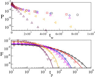
Figure 1: Top panel: probability distribution of the waiting time between subsequent jumps of the same particle, $P(t_{w})$. The lin-log plot clarifies that the distribution is exponential at high temperature and progressively deviates from this behaviour on cooling. Bottom panel: probability distribution of the time particles persist in their cages before making their first jump, $F(t_{p})$ (points), and prediction obtained from the CTRW model (lines), as in Eq. 1. The prediction has been obtained numerically integrating the data for $P(t_{w})$ in the top panel. In both panels the temperature is $T=2.5$, $2.2$, $2.0$, $1.9$, $1.8$, and $1.7\times 10^{-3}$, from left to right.

Figure 2 (main panel) shows the the fundamental timescales of the CTRW approach, $\langle t_{w}\rangle$ and $\langle t_{p}\rangle$, as a function of the temperature. As predicted by Eq. 1, $\langle t_{w}\rangle=\langle t_{p}\rangle$ at high temperature, where the waiting time distribution is indeed nearly exponential. Upon cooling, instead, the growth of temporal correlations leads to a decoupling between the two timescales. In particular, we find that $\langle t_{w}\rangle$ grows à la Arrhenius, while $\langle t_{p}(T)\rangle$ increases with a faster super–Arrhenius behavior. This can be understood considering that the waiting times from particles performing subsequent rapid jumps have a major weight on $\langle t_{w}\rangle$ but none on $\langle t_{p}\rangle$. Indeed this latter takes contributions only by the first jump of each particle and is therefore more affected by rare but very long waiting times.

A comparison with experimental results suggests that $\langle t_{w}\rangle$ and $\langle t_{p}\rangle$ correspond respectively to the $\beta$ and to the $\alpha$ relaxation time scales of structural glasses ^{1; 33; 45}, as we better motivate later on. Furthermore, the temperature $T_{x}\simeq 0.002$ where $\langle t_{w}\rangle$ and $\langle t_{p}\rangle$ firstly decouples marks the beginning of the Stokes-Einstein (SE) breakdown at the wavelength of the jump length²⁸, and, is akin of the onset temperature ³⁹.

Finally, the spatial features of the CTRW approach are fixed by the mean square jump length, $\langle\Delta r_{J}\rangle$ which decreases on cooling as illustrated in Fig.2 Inset.

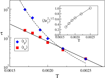
Figure 2: Temperature dependence of the average time particles persist in a cage before making the first jump, $\langle t_{p}\rangle$, and of the average cage duration, $\langle t_{w}\rangle$. $\langle t_{w}\rangle$ is well described by an Arrhenius $\langle t_{w}\rangle\propto\exp\left(A/T\right)$ (full line). $\langle t_{p}\rangle$ grows á super–Arrhenius law. The dashed line is a fit to $\langle t_{p}\rangle\propto\exp\left(A/T^{2}\right)$ but other functional forms, including the Vogel–Fulcher one, also describe the data. The inset illustrates the temperature dependence of the average jump length. The line is a guide to the eye.

3.1.2 CTRW predictions of macroscopic dynamics

We start showing that the macroscopic relaxation can be related to the statistical features of cage–jump motion focusing on the persistence correlation function, we define as the fraction $p$ of particles that has not jumped up to time $t$ ^{41; 42; 43; 44}.

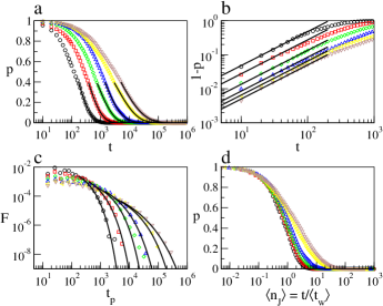
Figure 3: Panel a shows the decay of the persistence, together with stretched exponential fits of its long time behavior. Panel b illustrates the early time decay of the persistence. Lines correspond to $1-p(t)=t/\langle t_{w}\rangle$. Panel c compares $F(t_{p})$ with full lines derived from the stretched exponential fit to the persistence, see text. Panel d illustrates the dependence of the persistence on the average number of jumps per particle. In all panels the temperature is $T=2.5$, $2.2$, $2.0$, $1.9$, $1.8$, and $1.7\times 10^{-3}$, from left to right.

According to the CTRW framework, the persistence can be related to the distribution of the time $t_{p}$ particles persist in their cages before making the first jump, $p(t)=1-\int_{t_{p}=0}^{t}{F(t_{p})dt_{p}}$  ^{33; 45; 34}. The relation between $p$ and $F$ is illustrated in Fig. 3. At short times all jumps contribute to the decay of the persistence; consistently, we find $p(t)=1-t/\langle t_{w}\rangle$, as $\langle t_{w}\rangle^{-1}$ is the rate at which particles jump, and $F=-dp(t)/dt=\langle t_{w}\rangle^{-1}$. At long times we observe the persistence to decay with a stretched exponential, $p(t)\propto\exp\left(-(t/\tau)^{\beta}\right)$, and therefore expect $F(t_{p})=-dp(t)/dt\propto\tau^{-\beta}t^{\beta-1}\exp\left(-(t/\tau)^{\beta}\right)$, as verified in Fig. 3c. As usual in structural glasses, the stretched exponential exponent $\beta(T)$ decreases on cooling from its high temperature value, $\beta=1$. This decrement causes changes in the macroscopic dynamics, which can be highlighted considering the decay of the persistence as a function of the average number of jumps per particle, $\langle n_{J}(t)\rangle=t/\langle t_{w}\rangle$, as in Fig. 3d. The different curves collapse at small $\langle n_{J}\rangle$, as the short time dynamics is controlled by $\langle t_{w}\rangle$. Conversely, at a given average large number of jumps per particle, the lower the temperature the higher the value of the persistence, indicating the presence of growing temporal correlations between the jumps, with particles that have already jumped being more likely to perform subsequent jumps. In this respect, it is worth noticing that the CTRW approach neglects spatial correlations but encodes the presence of temporal heterogeneities in the form of the waiting time distributions.

The diffusion coefficient and the relaxation time of the self intermediate scattering functions (ISSF), which are commonly measured in experiments, can be also related to the statistical features of the cage–jump motion. For the diffusion constant $D$, the CTRW approach predicts $D=\langle\Delta r_{J}^{2}\rangle/\langle t_{w}\rangle$, as illustrated in Fig. 4(inset). The ISSF relaxation time $\tau_{\lambda}$ at a generic wavelength $\lambda$ (wavevector $2\pi/\lambda$), is expected to equals the average time a particle needs to move a distance $\lambda$, as in the CTRW approach this is simply the time particles need to perform, on average, $m_{\lambda}(T)=\lambda^{2}/\langle\Delta r^{2}_{J}(T)\rangle$ jumps. Accordingly, this time is fixed by the average first jump waiting time, $\langle t_{p}\rangle$, by the average cage duration, $\langle t_{w}\rangle$, and, by the average jump duration, $\langle\Delta t_{J}\rangle$,

$$\tau_{\lambda}\propto\langle t_{p}\rangle+(m_{\lambda}-1)\langle t_{w}\rangle+m_{\lambda}\langle\Delta t_{J}\rangle.$$ (2)

The last term is actually negligible at low temperatures, where $\langle t_{w}\rangle\gg\langle\Delta t_{J}\rangle$ ²⁶. Fig. 4 shows that this prediction agrees very well with the measured data in the investigated range of $\lambda$, with a coefficient of proportionality of the order of $1$. We remark that we have explored values of $\lambda$ ranging from $1$ to $4$ diameters of the largest component, corresponding to a relaxation time varying more than three decades.

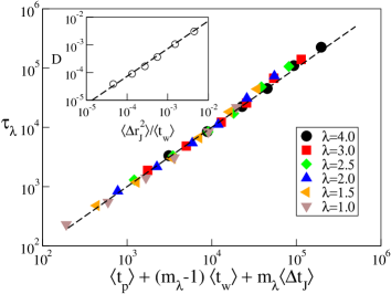
Figure 4: The relaxation time $\tau_{\lambda}$ at length scale $\lambda$ is directly related to the cage–jump properties, as in Eq. 2. $\lambda$ is measured in unit of the diameter of the largest particles. For each value of $\lambda$ we compare values of $\tau_{\lambda}$ measured at six different values of the temperature. The inset illustrates the diffusivity versus its prediction in terms of the cage jump properties.

Exploiting the dependence of the diffusivity and of the relaxation time on the jump properties, the breakdown of the Stokes–Einstein relation $\tau_{\lambda}\propto D^{-1}$ appears to be mainly controlled by the ratio of $\langle t_{p}(T)\rangle$ and $\langle t_{w}(T)\rangle$, but it is also affected by the temperature dependent jump length, differently to lattice models, where the step size is fixed. As a consequence, by equating the first two terms of the r.h.s. of Eq. 2, the length scale below which the breakdown of the SE relation occurs  ³³, $l\simeq\langle\Delta r^{2}_{J}\rangle^{1/2}(\langle t_{p}\rangle/\langle t_{w}\rangle)^{1/2},$ also depends on the jump length.

The relation of $\langle t_{p}(T)\rangle$ and $\langle t_{w}(T)\rangle$ with the macroscopic dynamics, supports their correspondence with the $\beta$ ($\langle t_{w}\rangle$) and the $\alpha$ ($\langle t_{p}\rangle$) relaxation timescales of structural glasses, as mentioned above.

3.1.3 Distribution of single-particle diffusivities

It is not possible to identify the dynamical phases from the van-Hove (vH) distribution of particle displacements (i.e. the probability that a particle has moved of a distance $r$ along a fixed direction) without introducing some empirical criteria, for instance by considering as ‘fast’ $5\%$ particles with the largest displacement¹⁵. This is because, if a fraction of the particles has a given diffusivity, then their vH distribution is a Gaussian distribution centered in zero, with variance proportional to the diffusivity. In the presence of two groups of particles with different diffusivities, the overall vH distribution is the weighted sum of two Gaussians with zero average, and it displays a single one maximum in zero, not the two ones required to a clear identification of the two phases. This clarifies that, in order to investigate whereas two or more dynamical phases coexist, one should investigate the diffusivity distribution, not the vH distribution. However, direct measurements of the diffusivity distribution are difficult. Furthermore, a direct inversion of the vH distribution can only be adopted^{46; 47}, if the diffusivity distribution is assumed to be time independent, as in systems with a unique and sharply defined timescale. Unfortunately this is not the case of glasses and different approaches are needed to tackle this problem.

In the CTRW approximation, the diffusivity of particles that have performed $n_{J}$ jumps at time $t$ is $d(n_{J},t)=n_{J}(t)\langle\Delta r^{2}_{J}\rangle/t$. The diffusivity is therefore simply proportional to the number of jumps per unit time, which can be easily monitored using our algorithm. Indeed, Fig.s 5 illustrates several features of the distribution of the number of jumps per particle rescaled by the average number of jumps $\langle n_{J}(t)\rangle=t/\langle t_{w}\rangle$, which coincides with the distribution of the single particle diffusion coefficient normalized by the average diffusion coefficient, $\langle d\rangle=D$. In Fig.s 5a and b we show these distributions at different times, respectively at the highest and lowest temperature we have considered.

At $t=0$, $P(n_{J};0)=\delta(n_{J})$ ($P(d;0)=\delta(d)$), as particles have not jumped; conversely, in the infinite time limit the distributions have a Gaussian shape with average value $\langle n_{J}(t)\rangle$ ($d=\langle d\rangle$). At high temperature, the distribution gradually broadens in time, and its maximum moves from $n_{J}\simeq 0$ to $n_{J}\simeq\langle n_{J}\rangle$. At low temperature, conversely, the distribution becomes bimodal, before reaching its asymptotic shape. This signals the coexistence of an immobile or low-diffusivity phase with particles having performed few or no jumps at all, and of a mobile or high-diffusivity phase, with particles having performed many jumps. We rationalize the appearance of a bimodal shaped distribution considering that $P(n_{J};t)$ is affected by the two timescales, $\langle t_{p}\rangle$ and $\langle t_{w}\rangle$. The slow timescale, $\langle t_{p}\rangle$, controls the value of the peak at $n_{J}=0$, that equals the persistence correlation function, $P(n_{J}=0;t)=p(t)$. The fast timescale, $\langle t_{w}\rangle$, controls the average value of the distribution, as the position of the second maximum asymptotically occurs at $n_{J}=t/\langle t_{w}\rangle$.

Figure 5c shows that the variance to mean ratio $\sigma^{2}_{n}/\langle n_{J}\rangle$ of $P(n_{J};t)$ approaches a plateau value at long time. We found that this time scales as $\langle t_{p}\rangle^{a}$, with $a\simeq 1.3$ (in general, $a\geq 1$ and it is model dependent)²⁷. The plateau value $g$ also grows on cooling. This is an other consequence of the growing temporal correlations controlled by the decoupling between $\langle t_{p}\rangle$ and $\langle t_{w}\rangle$. Indeed, the CTRW approach predicts that asimptotically $g\propto\langle t_{p}\rangle/\langle t_{w}\rangle$, consistently with our data (see Fig. 5d) .

It is worth noticing that a distribution with the long–time features of $P(n_{J};t)$, i.e. a Gaussian distribution with variance $\sigma^{2}_{n}=\langle n_{J}\rangle g$, is obtained by randomly assigning the jumps to the particles, in group of $g$ elements. Consistently, at the highest temperature, where correlations are negligible, $g=1$ and $P(n_{J};t)$ corresponds to that obtained by randomly assigning each jump to the particles, i.e. a Poisson distribution. The increase of $g$ on cooling indicates that at low temperature one might observe, in the same time interval, some particles to perform $g$ jumps, and other particles to perform no jumps at all, which illuminates the relation $g\propto\langle t_{p}\rangle/\langle t_{w}\rangle$. We remark that $g$ is a stationary quantity, as it holds constant in the infinite time limit.

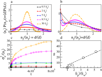
Figure 5: Panels a and b show the probability distribution of the number of jumps per particle rescaled by the average number of jumps, at $T=2.5\times 10^{-3}$ and at $T=1.7\times 10^{-3}$, respectively, and different times, as indicated. This distribution equals that of the single particle diffusion coefficient at different time, rescaled by the average diffusivity, as reported on the axes. Panel c illustrates the time evolution of the variance to mean ratio of this distribution. Different curves refer to different temperatures, as in Fig. 3, from bottom to top. Panel d is a plot of the asymptotic value of the variance to mean ratio, $g$, as a function of $\langle t_{p}\rangle/\langle t_{w}\rangle$. The dashed line is a guide to the eyes, $g\propto\langle t_{p}\rangle/\langle t_{w}\rangle$

3.2 Structure-dynamics correlations

We now show that, in the investigated system, the dynamical phase coexistence is accompanied by clear structural changes on cooling. These structural changes has been investigated focusing on the hexatic order parameter ⁴⁸, as the hexatic order is that expected to be relevant in our two dimensional system. The hexatic order parameter of particle $j$, $\psi_{6}^{j}$, is defined as:

$$\psi_{6}^{j}=\frac{1}{z_{j}}\sum_{m=0}^{z_{j}}e^{i6\theta^{j}_{m}},$$ (3)

where the sum runs over the $z_{j}$ neighbours of the particle $j$. We define two particles $m$ and $j$ to be neighbours if in contact, $|r_{mj}|<\sigma_{mj}$, where $\sigma_{mj}$ is their average diameter. $\theta_{m}$ is the angle between ${\bf r}_{mj}$ and a fixed direction (e.g. the $x$-axis). $|\psi_{6}^{j}(t)|$ has its maximum, $|\psi_{6}^{j}|=1$, if the neighbours of the particle $j$ are in a hexagonal order at time $t$, while $|\psi_{6}^{j}|=0$ for a random arrangement. We also associate to each particle its averaged order parameter, $\langle|\psi_{6}^{j}|\rangle_{t}$, where the average is computed in the time interval $[0:t]$. Note that we have considered the hexatic order parameter to identify structural heterogeneities, as this is the ordered characterizing two dimensional assemblies of soft disks. In different dimensionalities and for different potentials other order parameters, or the excess entropy, might be more appropriate ⁴⁸.

As illustrated in Fig. 6a, the single–particle hexatic order parameter has a bimodal distribution, that becomes more apparent on cooling. This signals the presence of a small fraction of highly ordered particles, and suggests that ordered and persistent particles might be related.

We show that this is actually the case investigating an overlap function $Q$ between ordered and persistent particles. In particular, we investigate the correlations between the set containing the $m=5\%$ most persistent particles and that containing the $m=5\%$ most ordered particles. The persistent particles set contains all the particles that have not jumped up to a time $t$, so that $p(t)=m$. The most ordered particles are those with the highest value of averaged order parameter $\langle|\psi_{6}^{j}|\rangle_{t}$. For the persistent particles, $n_{p}^{i}=1$. Similarly, we introduce a scalar $w_{\psi}^{i}$ to distinguish between the particles that are among the most ordered, $w_{p}^{i}=1$, and those that are not, $w_{\psi}^{i}=0$. The overlap between ordered and persistent particles is therefore defined as

$$Q(T)=\frac{(1/N)\sum_{i=0}^{N}n_{p}^{i}w_{\psi}^{i}-m^{2}}{m-m^{2}},$$ (4)

This function equals $Q=1$ when the two populations coincide, and $Q=0$ when they are uncorrelated. Fig. 6b shows that $\langle Q(T)\rangle$ increases on cooling, and thus demonstrates the existence of strong correlations between statics and dynamics ⁴⁸. Snapshots of the system in Fig.s 6c,d illustrate the meaning of $Q$, confirm that ordered and persistent particles largely overlap at low temperature, and also show that they form clusters. Since particles belonging to the core of these clusters can only jump after those of the periphery, the relaxation of these clusters is highly cooperative. At the level of the single particle cage–jump motion, this k–core ⁴⁹ like mechanism appears the one responsible for the decoupling of the two timescales, and for the emergence of dynamical heterogeneities. It is worth noticing that these highly ordered clusters look like micro-crystals, which are indeed likely to form in this systems, although full scale crystallization is suppressed.

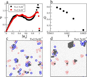
Figure 6: (a) Probability distribution of the hexatic order parameter, $P(|\psi_{6}|)$. (b) Temperature dependence of the average overlap between persistent and ordered particles. (c,d) Snapshots of a portion of the system at different temperatures, as indicated, and at times $t$ such that $p(t)=5\%$. The $5\%$ particles that have not yet jumped (thin red circles), and the $5\%$ with the highest averaged (from $0$ to $t$) hexatic order parameter (thick blue circles) are shown. Particles being simultaneously ordered and persistent are highlighted (filled circles).

4 Discussion

The CTRW approach completely neglects the presence of spatial correlations between jumps of different particles. Indeed, we recently showed that, for the model considered here, jumps actually occur in group of few particles²⁸. Moreover, for a correct CTRW description it is crucial to fairly identify elementary irreversible events. In the deeply supercooled regime this could become problematic, as subsequent jumps of a same particle are expected to become increasingly anti-correlated, in the form of back and forward moves. In that case, alternative definitions of local relaxation events or more sophisticated methods to distinguish irreversible jumps are needeed to properly describe the dynamics within a CTRW approach. For the system considered here, our algorithm successfully identifies irreversible jumps, at least in the temperature range allowed by simulations. Indeed, we have shown that the CTRW framework describes surprisingly well the dynamics of this atomistic glass-formers down to the lowest investigated temperature. In the 3D KA-LJ, small deviations from the CTRW predictions are only found at the lowest investigated temperature ²⁷.

Differences between glassy dynamics in two and three dimensions, whether fundamental or apparent, has been debated in very recent works ^{50; 51}, pointing out that dimensionality and system size lead to quantitative change in the cage-jumps properties. Despite of these differences, we have shown that our approach provides the same dynamical scenario in 2-D and 3-D systems, and a robust framework to connect the microscopic and the macroscopic dynamics.

The main success of this approach is the identification of two dynamical phases trough the bimodal shape of the diffusivity distribution. In the investigated 2D system, the dynamical phase coexistence is accompanied by a striking ”structural bimodal” of the hexatic order parameter, that is probably related to the presence of micro-crystals. The same clear structural signature is not observed in other standard glass formers, where local crystallization is completely suppressed. This can raise the suspect that the ”dynamic bimodal” distribution of diffusivities is directly triggered by that of the hexatic order, and thus it is a peculiar property of this systems as well. By contrast, we can claim that the temporary bimodal shape of the diffusivity distribution is a general property of glass formers, as for the standard 3D KA-LJ models we do observe a dynamical bimodality but not a structural bimodality²⁷, at least when the structure is investigated via crystalline-like order parameters. This demonstrates that the dynamical phase coexistence is not necessarily related to local crystallization, but does not exclude that correlations with different structural properties could exist. In general, it remains an open question whether the dynamical phase coexistence has a structural counterpart, or whether the reported structure-dynamics correlations must be considered as a by-product of particular models.

Acknowledgments
We acknowledge financial support from MIUR-FIRB RBFR081IUK, from the SPIN SEED 2014 project Charge separation and charge transport in hybrid solar cells, and from the CNR–NTU joint laboratory Amorphous materials for energy harvesting applications.

References

- 1 Debenedetti P G and Stillinger F H 2001 Nature 410 259
- 2 Berthier L and Biroli G 2011 Rev. Mod. Phys. 83 587
- 3 Cavagna A 2009 Phys. Rep. 476 51
- 4 Royall C P and Williams S R 2015 Phys. Rep. 560 1
- 5 Biroli G, Bouchaud J-P, Cavagna A, Grigera T S and Verrocchio P 2008 Nature Phys. 4 771
- 6 Biroli G, Cammarota C, Tarjus G and Tarzia M 2014 Phys. Rev. Lett. 112 175701
- 7 Mosayebi M, Del Gado E, Ilg P and Ottinger H G 2010 Phys. Rev. Lett. 104 205704
- 8 Berthier L, Biroli G, Bouchaud J-P, Cipeletti L, and van Saarloos W. 2011 Dynamical Heterogeneities in Glasses, Colloids, and Granular Media (Oxford: Oxford University Press)
- 9 Schmidt–Rohr K and Spiess H W 1991 Phys. Rev. Lett. 66 3020
- 10 Glotzer S C 2000 J. Non–Cryst. Solids 274 342
- 11 Ediger M D 2000 Annu. Rev. Phys. Chem. 51 99
- 12 Hedges L O, Jack R L, Garrahan J P and Chandler D 2009 Science 323 1309
- 13 Cammarota C, Cavagna A, Giardina I, Gradenigo G, Grigera T S, Parisi G and Verrocchio P. 2010 Phys. Rev. Lett. 105 055703
- 14 Speck T, Malins A and Royall C P 2012 Phys. Rev. Lett. 109 195703
- 15 Weeks E R, Crocker J C, Levitt A C, Schofield A and Weitz D A 2000 Science 287 627
- 16 Widmer-Cooper A, Harrowell P and Fynewever H 2004 Phys. Rev. Lett. 93 135701
- 17 Widmer–Cooper A and Harrowell P 2006 J. Non-Cryst. Solids 352 5098
- 18 Hocky G M, Coslovich D, Ikeda A and Reichman D R 2014 Phys. Rev. Lett. 113 157801
- 19 Appignanesi G A, Fris J A R, Montani R A and Kob W 2006 Phys. Rev. Lett. 96 057801
- 20 Vogel M, Doliwa B, Heuer A and Glotzer S C 2004 J. Chem. Phys. 120 4404
- 21 Carmi S, Havlin S, Song C, Wang K and Makse H A 2009 J. Phys. A: Math. Theor. 42 105101
- 22 Vollmayr-Lee K 2004 J. Chem. Phys. 121 4781
- 23 Helfferich J, Ziebert F, Frey S, Meyer H, Farago J, Blumen A and Baschnagel J 2014 Phys. Rev. E. 89 042603
- 24 Helfferich J, Ziebert F, Frey S, Meyer H, Farago J, Blumen A and Baschnagel J 2014 Phys. Rev. E. 89 042604
- 25 Pica Ciamarra M, Pastore R and Coniglio A 2016 Soft Matter DOI: 10.1039/C5SM01568E
- 26 Pastore R, Coniglio A and Pica Ciamarra M 2014 Soft Matter 10 5724
- 27 Pastore R, Coniglio A and Pica Ciamarra M 2015 Sci. Rep. 5, 11770
- 28 Pastore R, Coniglio A and Pica Ciamarra M 2015 Soft Matter 11 7214
- 29 Pastore R, Pesce G, Sasso A and Pica Ciamarra M 2015 Soft Matter 11 622
- 30 Montroll E W and Weoss G H 1965 J. Math. Phys. 6 167
- 31 Plimpton S J. Comp. Phys. 1995 117 1
- 32 Larini L, Ottochian A, De Michele C and Leporini D 2007 Nature Phys. 4 42
- 33 Berthier L, Chandler D and Garrahan J P Europhys. Lett. 2005 69 320
- 34 Jung Y, Garrahan J P and Chandler D 2004 Phys. Rev. E 69 061205
- 35 Feller W 1971 An Introduction to Probability Theory and its Applications Vol. 2, 2nd (New York: Wiley)
- 36 Tunaley J K E 1974 Phys. Rev. Lett. 33 1037
- 37 Lax M and Scher H 1977 Phys. Rev. Lett. 39 781
- 38 De Michele C and Leporini D 2001 Phys. Rev. E 63 036701
- 39 Keys A S, Hedges L O, Garrahan J P, Glotzer S C and Chandler D 2011 Phys. Rev. X 1 021013
- 40 Candelier R, Dauchot O and Biroli G 2009 Phys. Rev. Lett. 102 088001
- 41 Chandler D, Garrahan J P, Jack R L, Maibaum L and Pan A C 2006 Phys. Rev. E 74, 051501
- 42 Pastore R, Pica Ciamarra M, de Candia A and Coniglio A 2011 Phys. Rev. Lett. 107 065703
- 43 Pastore R, Pica Ciamarra A and Coniglio A 2013 Fractals 21 1350021
- 44 Chaudhuri P, Sastry S and Kob W 2008 Phys. Rev. Lett. 101 190601
- 45 Hedges L O, Maibaum L, Chandler D and Garrahan J P J. Chem. Phys. 2007 127 211101
- 46 Wang B, Kuo J, Bae S C and Granick S 2012 Nature Mat. 11 481
- 47 Sengupta S and Karmakar S 2014 J. Chem. Phys. 140 224505
- 48 Tanaka H, Kawasaki T, Shintani H and Watanabe K 2010 Nature Mat. 9 324
- 49 Bollobas B 1984 Graph Theory and Combinatorics: Proc. of the Cambridge Combinatorial Conf. in honour of Paul Erdos p. 35 (New York: Academic Press)
- 50 Flenner E and Szamel G 2015 Nature Comm. 6 7392
- 51 Shiba H, Kawasaki T and Kim K 2015 arXiv:1510.02546