Classical and quantum dynamics of a perfect fluid scalar-energy dependent metric cosmology

Abstract

Inspired from the idea of minimally coupling of a real scalar field to geometry, we investigate the classical and quantum models of a flat energy-dependent FRW cosmology coupled to a perfect fluid in the framework of the scalar-rainbow metric gravity. We use the standard Schutz’ representation for the perfect fluid and show that under a particular energy-dependent gauge fixing, it may lead to the identification of a time parameter for the corresponding dynamical system. It is shown that, under some circumstances on the minisuperspace prob energy, the classical evolution of the of the universe represents a late time expansion coming from a bounce instead of the big-bang singularity. Then we go forward by showing that this formalism gives rise to a Schrödinger-Wheeler-DeWitt (SWD) equation for the quantum-mechanical description of the model under consideration, the eigenfunctions of which can be used to construct the wave function of the universe. We use the resulting wave function in order to investigate the possibility of the avoidance of classical singularities due to quantum effects by means of the many-worlds and Bohmian interpretation of quantum cosmology.
PACS numbers: 98.80.Qc, 04.60.-m, 04.50.Kd
Keywords: Rainbow Cosmology, Quantum Cosmology, DSR theories

1 Introduction

One of the most important questions in cosmology is that of the initial conditions from which our present universe has began its evolution. As is well known, any answer to this question according to the standard model of cosmology based on the classical general relativity (GR), suffers from the existences of an initial singularity, the so-called big-bang singularity. Therefore, removing this initial singularity from the cosmological solutions of the Einstein’s equations is one of the most important challenges of GR and any hope to dealing with this issue would be in development of a quantum theory of gravity and consequently quantum cosmology (QC). In QC a common process to remove the big-bang is to replace it with a bounce in the sense that instead of initial singular ”bang”, the universe contracts until a minimal size (usually of the order of the Planck size $l_{Pl}$), bounces from this minimal size and then re-expands in such a way its late time behavior is given by classical cosmology. However, if one accepts that such a minimal size might be a fundamental quantity, with an eye to special relativity, this question may be arise: how is it possible to have a basic minimal length in nature which all inertia observers agree on its value. One may seek the answer to this question in one of the main motivations for the formation of an effective approach to QG knows as “Doubly Special Relativity” (DSR) [1, 2]. In DSR, in addition of the speed of light in standard SR, the non-linear representation of Lorentz transformations in momentum space gives an other global constant as Planck energy [3, 4, 5, 6, 7]. Concretely speaking, by fixing the natural cutoffs as planck length (or energy) DSR plays the role of a flat space-time limit of QG [8]. As a result, in the presence of the non-linear Lorentz symmetry, standard dispersion relations may be modified up to the leading order of Planck length [9, 10, 11, 12, 13]. A natural extension of DSR is when gravity (the curvature of space-time) comes into the play by which we are led to “ Doubly General Relativity” (DGR) or “gravity’s rainbow” which is based on two principles: the correspondence principle and the deformed equivalence principle [14]. The most important feature of this proposal which lead to breakdown of standard GR is that from the perspective of the particle(s) which is (are) exploring the space-time, the single classical geometry does not exist. This is a direct consequence of the disruption of the system under the measurement (here the geometry of space-time) by means of the measuring tools (here prob particle(s)). More technically, in the framework of the gravity’s rainbow, the geometry of space-time is described by a rainbow metric which itself is composed of one parameter family of the metrics which are functions of the energy of the prob particle(s). In the recent years, this semi-classical formalism of QG has attracted much attentions as far as various aspects of its cosmological implication has been studied, see [15]-[27].

In this paper we are going to extend a previously studied work on the perfect fluid scalar-metric cosmology [28], and investigate the classical and quantum dynamical evolution of a flat energy-dependent FRW cosmology with a perfect fluid matter source and a non-linear self-coupling scalar field minimally coupled to gravity’s rainbow. To express clear, in this work we would like to derive cosmological results in the presence of a naturally cutoff as Planck energy for FRW space-time metric. For the matter source of gravity, we consider a perfect fluid in Schutz’ formalism [29, 30]. The advantage of using this formalism is that after a canonical transformation the conjugate momentum associated to one of the variables of the fluid appears linearly in the Hamiltonian and so, in a natural way, it can offer a time parameter in terms of dynamical variables of the perfect fluid. Therefore, canonical quantization results in a Schrödinger-Wheeler-DeWitt (SWD) equation, in which this matter variable plays the role of time [31]-[34]. The paper has the following structure. In section 2, we present a brief review about the construction process of the rainbow geometry so that in the end we introduce the energy-dependent isotropic and homogeneous FRW space-time metric. In section 3, in terms of the Schutz’ time parameter, we shall obtain the classical dynamical behavior of the rainbow cosmic scale factor and the scalar field. We deal with the quantization of the model in section 4, and by computing the expectation values of the scale factor and the scalar field and also their Bohmian (ontological) counterparts in section 5, we show that the evolution of the universe according to the quantum picture is free of classical singularities. Section 6 is devoted to the summary and conclusions.

2 Rainbow geometry construction

As mentioned above, the main idea of DGR is based on the correspondence principle and the deformed equivalence principle. Therefore to construct the geometric structure corresponding to the rainbow scenario, checking these two principles is absolutely necessary. According to the correspondence principle, in the limit of low energy scales compared with $E_{Pl}$, the standard GR should be recovered. This means that

$$\lim_{\frac{E}{E_{Pl}}\rightarrow 0}g_{\mu\nu}(E)=g_{\mu\nu}~{}.$$ (1)

It should be noted that the dependence of the space-time metric on the energy may be interpreted as the energy scale in which the geometry of space-time is explored by means of test particle(s). Deformed equivalence principle, on the other hand, can be explained as: consider free falling observers in a region of space-time with a radius of curvature $R\gg l_{Pl}$, which measure physical objects such as particles and fields with energy $E$, the laws of physics are the same, provided that

$$R^{-1}\ll E\ll E_{Pl}~{}.$$ (2)

The above condition guarantees that based on DGR scenario, in the absence of the gravity (locally) DSR is recovered but not the standard SR. In summary, the deformed equivalence principle implies that in a region of the size $l_{Pl}$ around a given point of space-time, it is always possible to find a coordinate system in which the effects of gravity are negligible. Such a coordinate system is called “local deformed Lorentz frame”. By considering the above mentioned free falling observers as inertial observers in a rainbow flat space-time, we offer a family of local energy dependent orthonormal frame fields as

$$e_{0}=f_{1}^{-1}(\frac{E}{E_{Pl}})\tilde{e}_{0},~{}~{}~{}~{}~{}~{}e_{i}=f_{2}^{-1}(\frac{E}{E_{Pl}})\tilde{e}_{i},~{}~{}~{}(i=1,2,3)~{},$$ (3)

in which $\tilde{e}_{\mu}$ are the standard GR counterparts of $e_{\mu}$. Therefore, one gets the following flat metric for all inertial observers with various energies $E$

$$g(E)=\eta^{\mu\nu}e_{\mu}\otimes e_{\nu}~{}.$$ (4)

Here, $f_{1}$ and $f_{2}$ are two unknown energy dependent functions known as “rainbow functions” which according to the correspondence principle satisfy the limiting relations: $\lim_{\frac{E}{E_{Pl}}\rightarrow 0}f_{1,2}(\frac{E}{E_{Pl}})\rightarrow 1$. This means that in the low energy limit we have $e_{\mu}\rightarrow\tilde{e}_{\mu}$ which it seems to be quite reasonable. It is important to note that due to freedom in choosing the functions $f_{1,2}(\frac{E}{E_{Pl}})$, it is always possible to have functions with a strong damping as gaussian for example. This means that although we have introduced the interval (2) as an restriction on the energy of the probing particles, there is no reason to restrict the investigation with a cut-off at the Planck scale. Indeed, we may relax such a restriction and look for the rainbow particles with trans-Planckian energies [35]. Particulary, a gaussian profile for the rainbow functions can have physical implications, see for instance [35], in which by using of a variational viewpoint based on gaussian trial functionals, it is shown that some typical divergences can be controlled.

Metric (4) is known as flat DSR space-time or deformed Minkowski space-time and in terms of its components may be written as

$$dS^{2}=\frac{(dx^{0})^{2}}{f_{1}^{2}(\frac{E}{E_{Pl}})}-\frac{(dx^{i})^{2}}{f_{2}^{2}(\frac{E}{E_{Pl}})},$$ (5)

which $x^{0}$ and $x^{i}$ denote the time and spatial coordinates respectively.

Now, let us extend this issue to the cases in which the space-time metric has a dynamical behavior. By such an extension to a homogeneous and isotropic cosmological model, we may introduce the following energy-dependent (rainbow) FRW metric

$$dS^{2}=\frac{N^{2}(t)}{f_{1}^{2}(\varepsilon)}dt^{2}-\frac{a^{2}(t)}{f_{2}^{2}(\varepsilon)}\left[\frac{dr^{2}}{1-kr^{2}}+r^{2}d\vartheta^{2}+r^{2}\sin^{2}\vartheta d\varphi^{2}\right],$$ (6)

where, as usual, $N(t)$ is the lapse function, $a(t)$ the scale factor and $k=-1,0,1$ corresponds to the open, flat and closed universe respectively. Also, the the dimensionless parameter $0<\varepsilon<1$ is defined as $\varepsilon=\frac{E}{E_{Pl}}$.
In what follows, we will study the classical and quantum evolution of a FRW universe in its radiation dominate period in the context of rainbow gravity. To do this, due to the statistical nature of the very early universe, we take an ensemble of massless particles (like photons or gravitons) as prob particles of the space-time. In fact, we want to consider the average effect of these particles (which are moving on the space-time geometry) during a given measuring process. We will see that the average energy of the prob photons may vary or may be constant with the time evolution of universe. In the following sections, the implications of the both possibilities will be considered.

3 The classical cosmological model

Let us start with a FRW cosmological model whose metric is coupled with a scalar field. Also, the matter role of our model is played with a perfect fluid. The action of such a structure may be written as (we work in units where $c=\hbar=16\pi G=1$)

$${\cal S}=\int_{M}d^{4}x\sqrt{-g}\left[R-F(\phi)g^{\mu\nu}\phi_{,\mu}\phi_{,\nu}\right]+2\int_{\partial M}d^{3}x\sqrt{h}h_{ab}K^{ab}+\int_{M}d^{4}x\sqrt{-g}p,$$ (7)

where $R$ is the Ricci scalar and $F(\phi)$ is an arbitrary function of the scalar field $\phi$. Also, $K^{ab}$ and $h_{ab}$ are the extrinsic curvature and induced metric on the three-dimensional spatial hypersurfaces, respectively. The boundary term in (7) will be canceled by the variation of $\int_{M}d^{4}x\sqrt{-g}R$ . This is the reason for including a boundary term in the action of a gravitational theory. That such a boundary term is needed is due to the fact that $R$, the gravitational Lagrangian density contains second derivatives of the metric tensor, a nontypical feature of field theories. The third term of (7) represents the matter contribution to the total action where $p$ is the pressure of the fluid which together with its energy density $\rho$ obey the following equation of state

$$p=\omega\rho.$$ (8)

A more familiar expression for the action of a perfect fluid is the Hawking-Ellis action $S_{P.F.}=-\int d^{4}x\sqrt{-g}\zeta(1+\upsilon)$, in which $\zeta$ and $\upsilon$ are the fluid’s density and elastic potential (or internal energy) respectively [36]. By definition of the fluid’s energy density and pressure as $\rho=\zeta(1+\upsilon)$ and $p=\zeta^{2}\frac{d\upsilon}{d\zeta}$, it is shown in [36] that the variation of this action with respect to the metric yields the standard expression $T^{\mu\nu}=(\rho+p)U^{\mu}U^{\nu}+pg^{\mu\nu}$, for the energy-momentum tensor of a perfect fluid. However, according to what is shown in [29, 30], the same result may be obtained if one varies the action $\int d^{4}x\sqrt{-g}p$ with respect to the metric. In this respect, the matter part of the action as is written in terms of pressure in (7) is equivalent to the usual Hawking-Ellis formalism for the perfect fluid.

In this work we consider the equation of state parameter $\omega$ as a constant whose values vary between $-1\leq\omega\leq 1$. According to the Schutz’s formalism the fluid’s four-velocity can be expressed in terms of some thermodynamical potentials as [29, 30]

$$U_{\nu}=\frac{1}{\mu}(\epsilon_{,\nu}+\theta S_{,\nu}),$$ (9)

where $\mu$ and $S$ indicate the specific enthalpy and the specific entropy, respectively. Also, the variables $\epsilon$ and $\theta$ have no clear physical interpretation in this formalism. Note that the fluid’s four velocity should satisfy the normalization condition $U_{\nu}U^{\nu}=-1$. Now, considering the above action as a dynamical system in which the scale factor $a$, scalar field $\phi$ and fluid’s potentials are considered as independent dynamical variables, we can rewrite the gravitational part of the action (7) as

$${\cal S}_{g} = \int dt{\cal L}_{g}=\int dt\frac{Na^{3}}{f_{1}f_{2}^{3}}dt\left\{\bigg{(}R-\frac{f_{1}^{2}}{N^{2}}\dot{\phi}^{2}F(\phi)\bigg{)}\right.$$ (10)

$$\left.-\lambda\left[R-\frac{6}{N^{2}}\left(\frac{\ddot{a}}{a}+\frac{f_{1}^{2}\dot{a}^{2}}{a^{2}}+\frac{kf_{2}^{2}}{a^{2}}-\frac{\dot{N}\dot{a}}{Na}\right)\right]\right\}~{},$$

in which we have used the definition of the Ricci scalar in terms of the metric functions and their derivatives as a constraint. In this procedure the Lagrange multiplier $\lambda$ can be obtained by variation with respect to $R$, with the result $\lambda=\frac{Na^{3}}{f_{1}f_{2}^{3}}$. Thus, one obtains the following point-like Lagrangian for the gravitational part of the model

$${\cal L}_{g}=\frac{f_{1}}{f_{2}^{3}}\frac{6a\dot{a}^{2}}{N}+\frac{6kNa}{f_{1}f_{2}}-\frac{f_{1}}{Nf_{2}^{3}}F(\phi)\dot{\phi}^{2}a^{3}~{}.$$ (11)

Now, let us return to the matter part of the action (7) from which the Lagrangian density of the fluid takes the form

$${\cal L}_{m}=\frac{Na^{3}}{f_{1}f_{2}^{3}}p~{}.$$ (12)

By using of the first law of thermodynamics and following the standard Schutz’s description of the perfect fluid it can be shown that the fluid’s equation of state is of the form (see [28] for details)

$$p=\frac{\omega}{(\omega+1)^{\frac{\omega+1}{\omega}}}\mu^{\frac{\omega+1}{\omega}}e^{-\frac{S}{\omega}}~{}.$$ (13)

On the other hand if we use the expression $U_{\nu}=(\frac{N}{f_{1}(\varepsilon)},0,0,0)$ as the fluid’s four-velocity in the normalization condition $U_{\nu}U^{\nu}=-1$, we get

$$\mu=\frac{(\dot{\epsilon}+\theta\dot{S})}{N}f_{1}(\varepsilon)~{}.$$ (14)

Finally, using the above constraints and thermodynamical considerations for the fluid we find the Lagrangian density of the matter as

$${\cal L}_{m}=\frac{f_{1}^{\frac{1}{\omega}}}{f_{2}^{3}}N^{-\frac{1}{\omega}}a^{3}\frac{\omega}{(\omega+1)^{1+\frac{1}{\omega}}}\left(\dot{\epsilon}+\theta\dot{S}\right)^{1+1/\omega}e^{-\frac{S}{\omega}}~{}.$$ (15)

We are now in a situation to construct the Hamiltonian for the model. In terms of the conjugate momenta the Hamiltonian is given by

$$H=\dot{a}P_{a}+\dot{\phi}P_{\phi}+\dot{\epsilon}P_{\epsilon}+\dot{S}P_{S}-{\cal L}~{},$$ (16)

where $H=H_{g}+H_{m}$ and ${\cal L}={\cal L}_{g}+{\cal L}_{m}$. The momenta conjugate to each of the above variables can be obtained from the definition $P_{q}=\frac{\partial{\cal L}}{\partial\dot{q}}$ with the result

$$\left\{\begin{array}[]{ll}P_{a}=\frac{12f_{1}(\varepsilon)}{f_{2}^{3}(\varepsilon)}\frac{\dot{a}}{N}~{},\\ \\ P_{\phi}=-\frac{12f_{1}(\varepsilon)}{f_{2}^{3}(\varepsilon)}F(\phi)\dot{\phi}a^{3}~{},\\ \\ P_{\epsilon}=\frac{f_{1}^{\frac{1}{\omega}}(\varepsilon)}{f_{2}^{3}(\varepsilon)}N^{-\frac{1}{\omega}}a^{3}\frac{\omega(1+\frac{1}{\omega})}{(\omega+1)^{1+\frac{1}{\omega}}}\left(\dot{\epsilon}+\theta\dot{S}\right)^{\frac{1}{\omega}}e^{-\frac{S}{\omega}}~{},\\ \\ P_{S}=\frac{f_{1}^{\frac{1}{\omega}}(\varepsilon)}{f_{2}^{3}(\varepsilon)}N^{-\frac{1}{\omega}}a^{3}\frac{\omega(1+\frac{1}{\omega})\theta}{(\omega+1)^{1+\frac{1}{\omega}}}\left(\dot{\epsilon}+\theta\dot{S}\right)^{\frac{1}{\omega}}e^{-\frac{S}{\omega}}~{}.\end{array}\right.$$ (24)

With the help of these relations and also applying the canonical transformation [37]

$$T=-P_{S}e^{-S}P_{\epsilon}^{-(\omega+1)}~{},~{}~{}~{}~{}~{}~{}~{}P_{T}=P_{\epsilon}^{\omega+1}e^{S}~{},$$ (25)

expression (16) leads to

$$H=N{\cal H}=\frac{N}{f_{1}(\varepsilon)}\left[-\frac{f_{2}^{3}(\varepsilon)}{24a}p_{a}^{2}-\frac{6ka}{f_{2}(\varepsilon)}+\frac{f_{2}^{3}(\varepsilon)}{4F(\phi)a^{3}}P_{\phi}^{2}+\frac{f_{2}^{3\omega}(\varepsilon)}{a^{3\omega}}P_{T}\right]~{}.$$ (26)

The momentum $P_{T}$, which in comparison with the other momenta in the Hamiltonian function appears linearly, is the only remaining canonical variable associated with the matter.

The classical equations of motion are governed in the Hamiltonian formalism as

$$\left\{\begin{array}[]{ll}\dot{a}=\{a,H\}=-\frac{N}{12}\frac{P_{a}}{a}~{}\frac{f_{2}^{3}(\varepsilon)}{f_{1}(\varepsilon)}~{},\\ \\ \dot{P_{a}}=\{P_{a},H\}=N\left[-\frac{1}{24}\frac{P_{a}^{2}}{a^{2}f_{1}(\varepsilon)}+\frac{3f_{2}^{3}(\varepsilon)}{4F(\phi)a^{4}f_{1}(\varepsilon)}P_{\phi}^{2}+\frac{6k}{f_{1}(\varepsilon)f_{2}(\varepsilon)}+3\omega\frac{f_{2}^{3\omega}(\varepsilon)}{f_{1}(\varepsilon)}a^{-3\omega-1}P_{T}\right]~{},\\ \\ \dot{\phi}=\{\phi,H\}=\frac{Nf_{2}^{3}(\varepsilon)}{2F(\phi)a^{3}f_{1}(\varepsilon)}P_{\phi}~{},\\ \\ \dot{P_{\phi}}=\{P_{\phi},H\}=N\frac{f_{2}^{3}(\varepsilon)P_{\phi}^{2}}{4a^{3}f_{1}(\varepsilon)}\frac{F^{\prime}(\phi)}{F(\phi)^{2}}~{},\\ \\ \dot{T}=\{T,H\}=\frac{N}{a^{3\omega}}~{}\frac{f_{2}^{3\omega}(\varepsilon)}{f_{1}(\varepsilon)}~{},\\ \\ \dot{P_{T}}=\{P_{T},H\}=0~{}.\end{array}\right.$$ (38)

We also have the Hamiltonian constraint ${\cal H}=0$. Up to now, the cosmological setting, in view of the concerning issue of time, has been of course under-determined. Before dealing with the solutions of these equations we must decide on a choice of time parameter which at the classical level may be resolved by using the gauge freedom via fixing the gauge. A glance at the above equations shows that by choosing the gauge $N=\frac{f_{1}(\varepsilon)}{f_{2}^{3\omega}(\varepsilon)}a^{3\omega}$, we have $T=t$, which means that variable $T$ may play the role of time. Now, let us rewrite the equations of motion in the gauge $N=\frac{f_{1}(\varepsilon)}{f_{2}^{3\omega}(\varepsilon)}a^{3\omega}$ as

$$\left\{\begin{array}[]{ll}\dot{a}=-\frac{a^{3\omega-1}}{12}f_{2}^{3-3\omega}(\varepsilon)P_{a}~{},\\ \\ \dot{P_{a}}=-\frac{a^{3\omega-2}}{24}f_{2}^{-3\omega}(\varepsilon)P_{a}^{2}+\frac{3f_{2}^{3-3\omega}(\varepsilon)a^{3-3\omega}}{4F(\phi)a^{4}f_{1}(\varepsilon)}P_{\phi}^{2}+6ka^{3\omega}f_{2}^{-3\omega-1}(\varepsilon)+3\omega a^{-1}P_{0}~{},\\ \\ \dot{\phi}=\frac{a^{3\omega-3}f_{2}^{-3+3\omega}(\varepsilon)}{2F(\phi)}P_{\phi}~{},\\ \\ \dot{P_{\phi}}=\frac{F^{\prime}(\phi)}{4F}a^{3\omega-3}f_{2}^{3-3\omega}(\varepsilon)P(\phi)^{2}~{}.\end{array}\right.$$ (46)

Here, we take $P_{T}=P_{0}$=const. By eliminating $P_{\phi}$ from the two last equations of the above system we obtain

$$\frac{\ddot{\phi}}{\dot{\phi}}+\frac{1}{2}\frac{F^{\prime}(\phi)}{F(\phi)}\dot{\phi}+3(1-\omega)\left(\frac{\dot{f}_{2}(\varepsilon)}{f_{2}(\varepsilon)}+\frac{\dot{a}}{a}\right)=0~{},$$ (47)

which can easily be integrated to yield

$$\dot{\phi}^{2}F(\phi)=Ca^{6\omega-6}f_{2}^{6\omega-6}(\varepsilon)~{},$$ (48)

where $C$ is an integration constant. Also, if we remove the momenta from the system (46) we arrive at the differential form of the Hamiltonian constraint as

$$-6a^{1-3\omega}f_{2}^{3\omega-3}(\varepsilon)\dot{a}^{2}+\dot{\phi}^{2}F(\phi)f_{2}^{3\omega-3}(\varepsilon)a^{3-3\omega}-6kf_{2}^{-3\omega-1}(\varepsilon)a^{1+3\omega}+P_{0}=0~{}.$$ (49)

With the help of (48) this equation, for the flat case $k=0$, can be put into the form

$$\frac{da}{dt}=\sqrt{\frac{C}{6}f_{2}^{6\omega-6}(\varepsilon)a^{6\omega-4}+\frac{P_{0}}{6}f_{2}^{3-3\omega}(\varepsilon)a^{3\omega-1}}~{}.$$ (50)

Before integration of this equation we have to choose the functional form of the rainbow function $f_{2}(\varepsilon)$ in terms of scale factor $a$. However, rainbow functions are usually a function of the energy of the prob particles moving on the geometry of space-time. In [38], by considering the early universe as a thermodynamical system filled with prob photons at thermal equilibrium, the relation between the average energy $\bar{E}$ of the ensemble of prob photons and energy density $\rho$ of the universe is obtained as $\bar{E}=\frac{4{\cal C}}{3}\rho^{\frac{1}{4}}$ (${\cal C}$ is a constant). Therefore, with the rainbow function of the form $f_{2}(\varepsilon)=(1-\frac{E}{E_{Pl}})^{-1}$ offered in [6], we find

$$f(\rho)=\big{(}1-\frac{4{\cal C}}{3E_{Pl}}\rho^{\frac{1}{4}}\big{)}^{-1}~{}.$$ (51)

Finally, by replacing the the relation $\rho=\rho_{0}a^{-3(1+\omega)}$ equation (50) takes the form

$$\frac{da}{dt}=\sqrt{\frac{C}{6}a^{6\omega-4}+\frac{P_{0}}{6}a^{3\omega-1}+C\eta(1-\omega)a^{\frac{21}{4}\omega-\frac{19}{4}}+\frac{P_{0}\eta}{2}(\omega-1)a^{\frac{9}{4}\omega-\frac{7}{4}}}~{}.$$ (52)

Here, $\eta=\frac{4{\cal C}\rho_{0}^{\frac{1}{4}}}{3E_{Pl}}$ is a small constant. It is seen that this equation can not be solved analytically. In figure 1 (left), employing numerical methods, we have shown the approximate behavior of the scale factor $a(t)$ for typical values of the parameters. We see that the evolution of the universe begins with a big-bang singularity at $t=0$ and follows an expansion phase at late time of cosmic evolution. To understand the relation between the big-bang singularity of the scale factor $a\rightarrow 0$, and possible singularities of the scalar field like the blow up singularity $\phi\rightarrow\pm\infty$, let us find the classical trajectory in configuration space $(a,\phi)$, where the time parameter $t$ is eliminated.

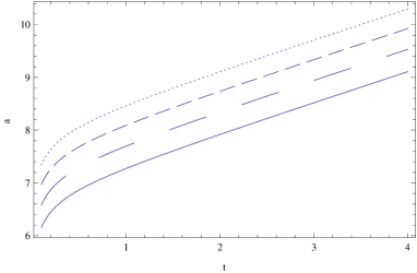
Figure 1: Left: The figure shows the time-behavior of the classical rainbow scale factor extracted from (52). The figure is plotted for the numerical values $\eta=0.001$, $\eta=0.0012$, $\eta=0.0014$ and $\eta=0.0016$ from down to up. Right: The classical trajectory in the plane $\phi-a$ for $\eta=0.001$, $\eta=0.002$, $\eta=0.003$ and $\eta=0.004$ from up to down. We set the numerical values $P_{0}=1$, $C=2$, with the EOS parameters $\omega=\frac{1}{3}$ for the period of the radiation dominate.

From (48), (49) one has

$$\frac{\sqrt{F(\phi)}d\phi}{da}=\frac{\sqrt{C}a^{3\omega-3}f_{2}^{3\omega-3}(\varepsilon)}{\sqrt{\frac{C}{6}f_{2}^{6\omega-6}(\varepsilon)a^{6\omega-4}+\frac{P_{0}}{6}f_{2}^{3-3\omega}(\frac{E}{E_{Pl}})a^{3\omega-1}}}~{}.$$ (53)

In the following, we shall consider the case of a power law coupling function in the form $F(\phi)=\lambda\phi^{n}$. With this choice for the function $F(\phi)$, equation (53) can be rewritten as

$$\frac{d\phi}{da}\phi^{n/2}=\frac{\sqrt{\frac{C}{\lambda}}a^{3\omega-3}+\sqrt{\frac{9C}{\lambda}}\eta(\omega-1)a^{\frac{9\omega-15}{4}}}{\sqrt{\frac{C}{6}a^{6\omega-4}+\frac{P_{0}}{6}a^{3\omega-1}+C\eta(1-\omega)a^{\frac{21\omega-19}{4}}+\frac{P_{0}\eta}{2}(\omega-1)a^{\frac{9\omega-7}{4}}}}~{}.$$ (54)

Again, due to the lack of an analytical solution, we have restricted ourself to a numerical solution which is plotted in figure 1 (right). As is clear from this figure the scalar field blows up when $a\rightarrow 0$ and tends to a constant value when $a\rightarrow\infty$.

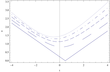
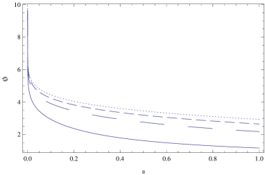
Figure 2: Left: The figure shows the classical scale factor (55) versus cosmic time for some values of $\varepsilon$: $\varepsilon=0.2$, $\varepsilon=0.4$, $\varepsilon=0.6$, $\varepsilon=0.8$ and $\varepsilon=1$ from down to up. Right: The classical trajectory (56) in the plane $\phi-a$ for the some values of $\varepsilon$: $\varepsilon=0.4$, $\varepsilon=0.6$, $\varepsilon=0.8$ and $\varepsilon=1$ from down to up. We set numerical values $P_{0}=1$, $C=2$, $\lambda=1$, $n=2$ with the EOS parameters $\omega=\frac{1}{3}$ for the period of the radiation dominate.

Now, let us consider an alternative case in which the average energy of prob photons remain constant. This assumption leads to the following solutions to the equations (50) and (53)

$$a=\sqrt{\frac{P_{0}}{6}(1+2\varepsilon)(t-\delta)^{2}-\frac{C}{P_{0}}~{}\left(\frac{1-4\varepsilon}{1+2\varepsilon}\right)},~{}~{}~{}~{}~{}\delta=\frac{\sqrt{6C}}{P_{0}}~{}\left(\frac{1-2\varepsilon}{1+2\varepsilon}\right)~{},$$ (55)

and

$$\phi=\left\{\sqrt{\frac{3}{2\lambda}}(n+2)\ln\left(\frac{\sqrt{\frac{C}{P_{0}}}(1-3\varepsilon)+\sqrt{\frac{C}{P_{0}}(1-3\varepsilon)^{2}+a^{2}}}{a}\right)\right\}^{\frac{2}{n+2}}~{},$$ (56)

where their behavior are plotted in figure 2. Note that for the low-energy test particles i.e. $E\ll E_{Pl}$, we have $f_{2}(\varepsilon)\rightarrow 1$ and $\eta\rightarrow 0$ and so from equations (48) and (52) we recover their standard counterparts as

$$\dot{\phi}^{2}F(\phi)=Ca^{6\omega-6}~{},$$ (57)

and

$$\frac{da}{dt}=\sqrt{\frac{C}{6}a^{6\omega-4}+\frac{P_{0}}{6}a^{3\omega-1}}~{},$$ (58)

which with the $\omega=\frac{1}{3}$ their solutions read as

$$a(t)=\sqrt{\frac{P_{0}}{6}(t-\delta)^{2}-\frac{C}{P_{0}}},\hskip 14.22636pt\delta=\frac{\sqrt{6C}}{P_{0}}~{},$$ (59)

and

$$\phi(a)=\left\{\sqrt{\frac{3}{2\lambda}}(n+2)\ln\left(\frac{\sqrt{\frac{C}{P_{0}}}+\sqrt{\frac{C}{P_{0}}+a^{2}}}{a}\right)\right\}^{\frac{2}{n+2}}~{}.$$ (60)

These solutions also exhibit similar singularities as we have already discussed when we were dealing with more general cases in figures 1 and 2. In the next sections we will see how this picture may be modified if one takes into account the quantum mechanical considerations in the problem at hand.

4 Quantization of the model

Let us now focus attention on the quantization of the model described above. The starting point will be the Wheeler-DeWitt (WDW) equation extracted from the super Hamiltonian (26). Since the lapse function plays the role of a Lagrange multiplier, so we have the classical constraint equation ${\cal H}=0$. In order to quantization of the minisuperspace we use the operator version of this constraint applying on the wave function $\Psi(a,\phi,T)$. For a flat FRW model this procedure yields

$${\cal H}\Psi(a,\phi,T)=\left[-\frac{1}{24}\frac{P_{a}^{2}}{a}+\frac{1}{4F(\phi)a^{3}}P_{\phi}^{2}+f_{2}^{3\omega-3}(\varepsilon)\frac{P_{T}}{a^{3\omega}}\right]\Psi(a,\phi,T)=0~{}.$$ (61)

A look at this relation shows that the ordering $a^{-1}P_{a}^{2}=P_{a}a^{-1}P_{a}$ and $F(\phi)^{-1}P_{\phi}^{2}=P_{\phi}F(\phi)^{-1}P_{\phi}$ makes the Hamiltonian Hermitian. So, by using of the standard representation $(P_{a},P_{\phi},P_{T})\rightarrow-i(\frac{\partial}{\partial a},\frac{\partial}{\partial\phi},\frac{\partial}{\partial T})$, we arrive at the Schrödinger-Wheeler-deWitt (SWD) equation as

$$\frac{1}{a}\frac{\partial^{2}\Psi(a,\phi,T)}{\partial a^{2}}-\frac{1}{a^{2}}\frac{\partial\Psi(a,\phi,T)}{\partial a}-\frac{6}{a^{3}F(\phi)}\frac{\partial^{2}\Psi(a,\phi,T)}{\partial\phi^{2}}+$$

$$\frac{6}{a^{3}}\frac{F^{\prime}(\phi)}{F(\phi)^{2}}\frac{\partial\Psi(a,\phi,T)}{\partial\phi}-\frac{24i}{a^{3\omega}}f_{2}^{3\omega-3}(\varepsilon)\frac{\partial\Psi(a,\phi,T)}{\partial T}=0~{}.$$ (62)

We separate the variables in this equation as

$$\Psi(a,\phi,T)=e^{iET}\chi(a,\phi)~{},$$ (63)

by which, equation (4) becomes

$$\frac{\partial^{2}\chi(a,\phi)}{\partial a^{2}}-\frac{1}{a}\frac{\partial\chi(a,\phi)}{\partial a}-\frac{6}{a^{2}F(\phi)}\frac{\partial^{2}\chi(a,\phi)}{\partial\phi^{2}}+$$

$$\frac{6}{a^{2}}\frac{F^{\prime}(\phi)}{F(\phi)^{2}}\frac{\partial\chi(a,\phi)}{\partial\phi}-24Ea^{3-3\omega}f_{2}^{3\omega-3}(\varepsilon)\chi(a,\phi)=0~{}.$$ (64)

Note that here $E$ is a separation constant which due to the assumption of constant average energy for the prob particles can be interpreted as the scale at which the minisuperspace is searching. The solutions of the above differential equation are separable and may be written in the form $\psi(a,\phi)=U(a)W(\phi)$ which yields

$$a^{2}\frac{d^{2}U(a)}{da^{2}}-a\frac{dU(a)}{da}+\bigg{(}24Ef_{2}^{3\omega-3}(\varepsilon)a^{3-3\omega}+m^{2}\bigg{)}U(a)=0~{},$$ (65)

and

$$\frac{6}{F(\phi)}\frac{d^{2}W(\phi)}{d\phi^{2}}-\frac{6F^{\prime}(\phi)}{F(\phi)^{2}}\frac{dW(\phi)}{d\phi}+m^{2}W(\phi)=0~{},$$ (66)

where $m$ is another constant of separation. It is seen that the scalar field part of the wave function is not affected by the rainbow function. On the other hand, by choosing the rainbow function $f_{2}(\varepsilon)=(1-\frac{E}{E_{Pl}})^{-1}$, the differential equation (65) can be rewritten as

$$a^{2}\frac{d^{2}U(a)}{da^{2}}-a\frac{dU(a)}{da}+\bigg{[}\bigg{(}24E-\frac{48E^{2}}{E_{Pl}}\bigg{)}a^{2}+m^{2}\bigg{]}U(a)=0,$$ (67)

whose general solution may be given in terms of the Bessel functions as

$$U(a)=a\left[c_{1}J_{\sqrt{1-m^{2}}}\left(\sqrt{24E-\frac{48E^{2}}{E_{Pl}}}a\right)+c_{2}Y_{\sqrt{1-m^{2}}}\left(\sqrt{24E+\frac{48E^{2}}{E_{Pl}}}a\right)\right].$$ (68)

Also, with $F(\phi)=\lambda\phi^{n}$, equation (66) has exact solution as

$$W(\phi)=\phi^{\frac{n+1}{2}}\left[c_{3}J_{\frac{n+1}{n+2}}\left(\frac{m\sqrt{6\lambda}}{3(n+2)}\phi^{\frac{n+2}{2}}\right)+c_{4}Y_{\frac{n+1}{n+2}}\left(\frac{m\sqrt{6\lambda}}{3(n+2)}\phi^{\frac{n+2}{2}}\right)\right]~{}.$$ (69)

Since the Bessel function $Y_{\nu}(z)$ has not a well-defined behavior near $z\approx 0$, we may set $c_{2}=c_{4}=0$. Therefore, the eigenfunctions of the SWD equation will be

$$\Psi_{mE}(a,\phi,T)=e^{iET}a\phi^{\frac{n+1}{2}}J_{\sqrt{1-m^{2}}}\left(\sqrt{24E-\frac{48E^{2}}{E_{Pl}}}a\right)J_{\frac{n+1}{n+2}}\left(\frac{m\sqrt{6\lambda}}{3(n+2)}\phi^{\frac{n+2}{2}}\right)~{}.$$ (70)

We note that if we restricted ourselves to the real values of the Bessel function’s argument, i.e. $24E-\frac{48E^{2}}{E_{Pl}}\geq 0$, an energy cut-off appears as $E\leq\frac{E_{Pl}}{2}$. Now, the general solution to the SWD equation may be written as a superposition of its eigenfunctions, that is

$$\Psi(x,y,T)=\int_{E=0}^{\infty}\int_{m=0}^{1}B(E)C(m)\Psi_{mE}(x,y,T)dEdm~{},$$ (71)

where $B(E)$ and $C(m)$ are suitable weight functions to construct the wave packets. To consider the effects of the energy’s cut-off on the above wave function, we re-scale the energy as $dE\rightarrow(1-\frac{E}{E_{Pl}})^{-1}dE$, so that the relation (71) takes the form

$$\Psi(x,y,T)=\int_{m=0}^{1}(I_{1}+I_{2})C(m)dm~{},$$ (72)

in which

$$I_{1}=\int_{E=0}^{\infty}B(E)\Psi_{mE}(x,y,T)dE,~{}~{}~{}~{}~{}~{}I_{2}=\frac{1}{E_{Pl}}\int_{E=0}^{\infty}EB(E)\Psi_{mE}(x,y,T)dE~{}.$$ (73)

The above integrals may be evaluated to find analytical expression if we choose the function $B(E)$ to be a quasi-Gaussian weight factor

$$B(E)=12\left(\sqrt{24E(1-\frac{2}{E_{Pl}})}\right)^{\sqrt{1-m^{2}}}\exp\left(-24E(1-\frac{2}{E_{Pl}})\right)~{},$$ (74)

in which we also have used the approximation $24E-\frac{48E^{2}}{E_{Pl}}\approx 24E(1-\frac{2}{E_{Pl}})$. By using the equalities [39]

$$\int_{0}^{\infty}e^{-az^{2}}z^{\nu+1}J_{\nu}(bz)dz=\frac{b^{\nu}}{(2a)^{\nu+1}}e^{-\frac{b^{2}}{4a}}~{},~{}~{}~{}~{}\int_{0}^{\infty}e^{-az^{2}}z^{\nu+3}J_{\nu}(bz)dz=\frac{b^{\nu}\left[-b^{2}+4a(1+\nu)\right]}{(2a)^{\nu+3}}e^{-\frac{b^{2}}{4a}}~{},$$ (75)

the result is

$$I_{1} = (1+\frac{2}{E_{Pl}})a\phi^{\frac{n+1}{2}}J_{\frac{n+1}{n+2}}\left(\frac{m\sqrt{6\lambda}}{3(n+2)}\phi^{\frac{n+2}{2}}\right)\left[a^{\sqrt{1-m^{2}}}\left(2-\frac{iT}{12}-\frac{iT}{6E_{Pl}}\right)^{-1-\sqrt{1-m^{2}}}\right.$$ (76)

$$\left.\exp\left(-\frac{a^{2}}{\left(4-\frac{iT}{6}-\frac{iT}{3E_{Pl}}\right)}\right)\right]~{},$$

and

$$I_{2} = \frac{1}{24E_{Pl}}a\phi^{\frac{n+1}{2}}J_{\frac{n+1}{n+2}}\left(\frac{m\sqrt{6\lambda}}{3(n+2)}\phi^{\frac{n+2}{2}}\right)\left[a^{\sqrt{1-m^{2}}}\left(2-\frac{iT}{12}-\frac{iT}{6E_{Pl}}\right)^{-3-\sqrt{1-m^{2}}}\right.$$ (77)

$$\left.\exp\left(-\frac{a^{2}}{\left(4-\frac{iT}{6}-\frac{iT}{3E_{Pl}}\right)}\right)\left(a^{2}+(1+\sqrt{1-m^{2}})\left(4-\frac{iT}{6}-\frac{iT}{3E_{Pl}}\right)\right)\right]~{}.$$

By means of these relations in (72), we have

$$\Psi(a,\phi,T) = \left\{(1+\frac{2}{E_{Pl}})\left(2-\frac{iT}{12}-\frac{iT}{6E_{Pl}}\right)^{-1-\gamma}+\frac{1}{24E_{Pl}}\left(2-\frac{iT}{12}-\frac{iT}{6E_{Pl}}\right)^{-3-\gamma}\right.$$ (78)

$$\left.\left(-a^{2}+(1+\gamma)\left(4-\frac{iT}{6}-\frac{iT}{3E_{Pl}}\right)\right)\right\}a^{1+\gamma}\exp\left(-\frac{a^{2}}{\left(4-\frac{iT}{6}-\frac{iT}{3E_{Pl}}\right)}\right)$$

$$\times\phi^{\frac{n+2}{2}}\int_{0}^{1}C(m)J_{\frac{n+1}{n+2}}\left(\frac{m\sqrt{6\lambda}}{3(n+2)}\right)dm~{}.$$

To obtain an analytical closed expression for the wave function, what remains is evaluation of the integral over $m$. At this step we assume that the above superposition is taken over such values of $m$ for which one can use the approximation $\sqrt{1-m^{2}}=\gamma$. Now, by choosing the weight function

$$C(m)=m^{\frac{2n+3}{n+2}}~{},$$ (79)

where $n$ is an arbitrary constant, and using the equality [39]

$$\int_{0}^{1}m^{r+1}J_{r}(zm)dm=\frac{J_{r+1}(z)}{z}~{},$$ (80)

we are led to the following expression for the (radiation dominated) wave function

$$\Psi(a,\phi,T) = 2\left(\frac{\sqrt{6\lambda}}{3(n+1)}\right)^{-1}\phi^{-\frac{1}{2}}a^{1+\gamma}\exp\left(-\frac{a^{2}}{\left(4-\frac{iT}{6}-\frac{iT}{3E_{Pl}}\right)}\right)$$ (81)

$$\times J_{\frac{2n+3}{n+2}}\left(\frac{m\sqrt{6\lambda}}{3(n+2)}\phi^{\frac{n+2}{2}}\right)\left\{(1+\frac{2}{E_{Pl}})\left(2-\frac{iT}{12}-\frac{iT}{6E_{Pl}}\right)^{-1-\gamma}\right.$$

$$\left.-\frac{a^{2}}{24E_{Pl}}\left(2-\frac{iT}{12}-\frac{iT}{6E_{Pl}}\right)^{-3-\gamma}\right\}~{}.$$

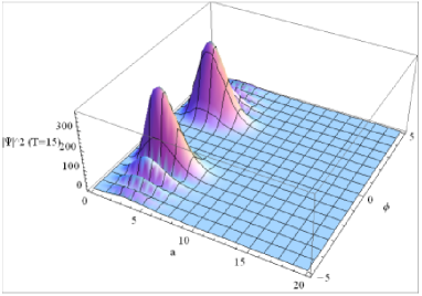
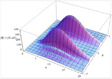
Figure 3: The probability density functions $|\Psi(a,\phi,T)|^{2}$ for the wave function (81) in four different time parameter $T=0,15,30,45$ with the numerical values $\gamma=0.25$, $n=2$, $\lambda=2$ and $E_{Pl}=1$.

In figure 3, we have plotted the probability densities correspond to the wave function (81) for typical numerical values of the parameters. As this figure shows, at $T=0$, the wave function has two dominant peaks in the vicinity of some non-zero values of scale factor and scalar field. This means that the wave function predicts the emergence of the universe from a quantum state corresponding to one of its dominant peaks. However, the emergence of several peaks in the wave packet may be interpreted as a representation of different quantum states that may communicate with each other through tunneling. In the other words, there are different possible states from which our present universe could have evolved and tunneled in the past, from one universe (state) to another. As time grows, the wave packet begins to propagate in the $a$-direction, its width becoming wider and its peaks moving with a group velocity towards the greater values of scale factor while the values of scalar field remain almost constant. The wave packet disperses as time passes, the minimum width being attained at $T=0$. As in the case of the free particle in quantum mechanics, the more localized the initial state at $T=0$, the more rapidly the wave packet disperses. Therefore, the quantum effects make themselves important only for small enough $T$ corresponding to small $a$, as expected and the wave function predicts that the universe will undergo into the states with larger $a$ and an almost constant $\phi$ in its late time evolution. If we turn off the rainbow’s effects in the wave function (see figure 1 of [28]), after examining the same numerical process, we verify that while the general behavior of the wave function is repeated, the rainbow model will go into its classical regime faster than the ordinary FRW model. This may be a consequence of the existence of a natural cutoff as $E_{Pl}$, in the metric.

Up to now, from our starting point to separate the variables in (63), we assumed that the parameter $E$ is a constant interpreted as the constat average energy of the ensemble of photons. In other words, here the source of $E$ comes from perfect fluid composed of photons with constant average energy and thus one can interpret it as the scale at which the minisuperspace is measuring. Now, we may relax this assumption and let such an energy scale can be changed. If so, we are not allowed to identity the separation constant (the oscillatory exponential term in equation (63)) with the energy scale by which the minisuperspace is probing. To handle this issue, let us do a slight change in notation and show the separation constant appeared in (63) with $\tilde{E}$ which from now on should be distinguished from the energy of the probing photons. So, by putting the rainbow function into (4), equation (65) can be rewritten as

$$a^{2}\frac{d^{2}U(a)}{da^{2}}-a\frac{dU(a)}{da}+\bigg{(}24\tilde{E}a^{2}+48\eta\tilde{E}a+m^{2}\bigg{)}U(a)=0~{}.$$ (82)

Note that, only the scale factor part of $\chi(a,\phi)$ is affected by the above assumption. The general solution of the differential equation (82) may be written as

$$U(a)=a^{\delta}\exp\left(\sqrt{-96\tilde{E}}a\right){\cal J}\left(-\frac{1}{2}+\delta-\eta\sqrt{-6\tilde{E}},~{}2\delta-1;~{}\frac{a}{2\sqrt{-96\tilde{E}}}\right),$$ (83)

where $\delta=1\pm\sqrt{1-m^{2}}$ and ${\cal J}(\alpha,\beta;z)$ is a degenerate hypergeometric function. For negative values of $\tilde{E}$, $\tilde{E}<0$, this expression has not a well-defined asymptotic behavior for large values of the variable $a$. Thus we consider $\tilde{E}>0$, for which with assumption $\eta\ll 1$, we have

$$U(a)=a^{\delta}\exp\left(i\sqrt{96\tilde{E}}a\right){\cal J}\left(-\frac{1}{2}+\delta,~{}2\delta-1;~{}\frac{-ia}{2\sqrt{96\tilde{E}}}\right).$$ (84)

By using of the following representations of the Bessel function $J_{\nu}(z)$ in terms of the degenerate hypergeometric functions [39]

$$J_{\nu}(z)=\frac{1}{\Gamma(\nu+1)}(z/2)^{\nu}\exp(-iz){\cal J}\left(\nu+\frac{1}{2},~{}2\nu+1;~{}2iz\right),$$ (85)

the solution (84) reads as

$$U(a)=\Gamma(\delta)a\left(-\frac{1}{8\sqrt{96\tilde{E}}}\right)^{1-\delta}\exp\left(i\sqrt{96\tilde{E}}a\right)\exp\left(\frac{-ia}{4\sqrt{96\tilde{E}}}\right)J_{\delta-1}\left(-\frac{a}{4\sqrt{96\tilde{E}}}\right)~{}.$$ (86)

Therefore, the eigenfunctions of the SWD equation are given by

$$\Psi_{m\tilde{E}}(a,\phi,T) = e^{i\tilde{E}T}a\phi^{\frac{n+1}{2}}\Gamma(1\pm\sqrt{1-m^{2}})\left(-\frac{1}{4\sqrt{96\tilde{E}}}\right)^{\mp\sqrt{1-m^{2}}}\exp\left(i\sqrt{96\tilde{E}}a\right)$$ (87)

$$\times\exp\left(\frac{-ia}{4\sqrt{96\tilde{E}}}\right)J_{\pm\sqrt{1-m^{2}}}\left(-\frac{a}{4\sqrt{96\tilde{E}}}\right)J_{\frac{n+1}{n+2}}\left(\frac{m\sqrt{6\lambda}}{3(n+2)}\phi^{\frac{n+2}{2}}\right)~{}.$$

As before, a superposition over the parameters $\tilde{E}$ and $m$ is needed to construct the wave function, that is

$$\Psi(a,\phi,T)=\int_{\tilde{E}=0}^{\infty}\int_{m=0}^{1}B(\tilde{E})C(m)\Psi_{m\tilde{E}}(a,\phi,T).$$ (88)

To evaluate the integral over $\tilde{E}$ and get an analytic expression we do it under approximations $T\tilde{E}\ll 1$ and $a\sqrt{96\tilde{E}}\ll 1$ which result in $e^{i\tilde{E}T}\approx 1+i\tilde{E}T$ and $e^{i\sqrt{96\tilde{E}}a}\approx 1$. By such approximations we may offer the weight function $B(\tilde{E})$ as

$$B(z)=768a^{\mu}\exp(-\frac{a}{4})\exp\left(-a(z+\frac{i}{2})^{2}\right)z^{6\pm 2\sqrt{1-m^{2}}},~{}~{}~{}~{}z=-\frac{1}{4\sqrt{96\tilde{E}}},$$ (89)

where $\mu$ is a positive constant. Under this condition we are led to the final form for the wave function as

$$\Psi(a,\phi,T) = \Gamma(1+\gamma)\phi^{-\frac{1}{2}}\left(\frac{\sqrt{6\lambda}}{3(n+1)}\right)^{-1}\exp(-\frac{a}{2})\left\{\left(\frac{1+\gamma}{2}\right)a^{\mu-1}+\left(\frac{iT}{3072}-4\right)a^{\mu}\right\}$$ (90)

$$\times J_{\frac{2n+3}{n+2}}\left(\frac{m\sqrt{6\lambda}}{3(n+2)}\phi^{\frac{n+2}{2}}\right),$$

in which we have taken again the integral over $m$ by approximation $\sqrt{1-m^{2}}=\gamma$ and with the weight function (79). A qualitative investigation of the wave function (90) shows that it has the same behavior as the figure 3, but with different (smaller) spreading rate.

Now, having the above wave functions let us see how the classical solutions may be recovered. In quantum cosmology, one usually constructs a coherent wave packet with good asymptotic behavior in the minisuperspace, peaking in the vicinity of the classical trajectory. So, to show the correlations between classical and quantum pattern, following the many-worlds interpretation of quantum mechanics [40], one may calculate the time dependence of the expectation value of the scale factor as

$$<a>_{T}=\frac{\int_{a=0}^{\infty}\int_{\phi=-\infty}^{\infty}\Psi^{*}a\Psi dad\phi}{\int_{a=0}^{\infty}\int_{\phi=-\infty}^{\infty}\Psi^{*}\Psi dad\phi}~{},$$ (91)

which yields

$$<a>_{T}=\frac{A_{1}\bigg{(}16+\frac{T}{36}+\frac{T}{9E_{Pl}}\bigg{)}-A_{2}\bigg{(}16+\frac{T}{36}+\frac{T}{9E_{Pl}}\bigg{)}^{2}}{A_{3}\bigg{(}16+\frac{T}{36}+\frac{T}{9E_{Pl}}\bigg{)}^{1/2}-A_{4}\bigg{(}16+\frac{T}{36}+\frac{T}{9E_{Pl}}\bigg{)}^{-5/2}}~{},$$ (92)

with

$$A_{1}=\bigg{(}\frac{3}{2}+\frac{3}{8E_{Pl}}\bigg{)},~{}~{}~{}A_{2}=\frac{1}{32E_{Pl}},~{}~{}~{}A_{3}=\sqrt{\frac{9\pi}{2}}A_{1},~{}~{}~{}A_{4}=\frac{2}{17}A_{2}~{},$$ (93)

for the wave function (81) with $\gamma=1$, and

$$<a>_{T}=\frac{(\frac{1+\gamma}{2})^{2}+\left(\frac{T^{2}}{1572864}+96\right)-8(1+\gamma)}{(\frac{1+\gamma}{2})^{2}+\left(\frac{T^{2}}{4718592}+32\right)-4(1+\gamma)}~{},$$ (94)

for the wave function (90). In view of the existence of singularities, these expectation values never vanish, showing that the corresponding quantum states are nonsingular. Indeed, the expression (92) and (94) represent a bouncing universe with no singularity where its late time behavior is almost the same as classical solution shown in figure 1. Also, the expectation value of the scalar field reads as

$$<\phi>_{T}=\frac{\int_{a=0}^{\infty}\int_{\phi=-\infty}^{\infty}\Psi^{*}\phi\Psi dad\phi}{\int_{a=0}^{\infty}\int_{\phi=-\infty}^{\infty}\Psi^{*}\Psi dad\phi},$$ (95)

with the result

$$<\phi>_{T} = \frac{\int_{-\infty}^{+\infty}z^{-\frac{n}{n+2}}J_{\frac{2n+3}{n+2}}^{{}^{\star}}\left(\frac{\sqrt{6\lambda}}{3(n+2)}z\right)\times J_{\frac{2n+3}{n+2}}\left(\frac{\sqrt{6\lambda}}{3(n+2)}z\right)dz}{\int_{-\infty}^{+\infty}z^{-1}J_{\frac{2n+3}{n+2}}^{{}^{\star}}\left(\frac{\sqrt{6\lambda}}{3(n+2)}z\right)\times J_{\frac{2n+3}{n+2}}\left(\frac{\sqrt{6\lambda}}{3(n+2)}z\right)dz}=$$ (96)

$$\frac{\Gamma(\frac{n}{n+1})\Gamma(\frac{3n+5}{n+2})\Gamma(2n+4)}{2^{\frac{n}{n+2}}\left(\Gamma(\frac{n+1}{n+2})\right)^{2}\Gamma(\frac{2n+3}{n+2})\Gamma(\frac{3n+4}{n+2})}\left(\frac{\sqrt{6\lambda}}{3(n+2)}\right),$$

where $z=\phi^{\frac{n+2}{2}}$. We see that the expectation value of $\phi$ is a time independent constant which is just the behavior predicted by the wave function of the SWD equation in figure 3.

5 Bohmian interpretation of quantum cosmological model

In this section we are going to study the classical behavior of the dynamical variables $a$ and $\phi$ in the framework of Bohmian quantum mechanics, according which the general form of the wave function may be written as

$$\Psi(a,\phi,T)=\Omega(a,\phi,T)e^{iS(a,\phi,T)},$$ (97)

where $\Omega$ and $S$ are some real function. Substitution of this expression into the SWD equation (4) leads to the continuity equation

$$2a^{2}\frac{\partial\Omega}{\partial a}\frac{\partial S}{\partial a}+a^{2}\Omega\frac{\partial^{2}S}{\partial a^{2}}+a\Omega\frac{\partial S}{\partial a}-\frac{12}{F(\phi)}\frac{\partial\Omega}{\partial\phi}\frac{\partial S}{\partial\phi}-\frac{6}{F(\phi)}\Omega\frac{\partial^{2}S}{\partial\phi^{2}}+6\frac{F^{\prime}(\phi)}{F(\phi)^{2}}\Omega\frac{\partial S}{\partial\phi}-24a^{2}\frac{\partial\Omega}{\partial T}=0,$$ (98)

and the modified Hamilton-Jacobi equation

$$-\frac{1}{24}\frac{1}{a}\left(\frac{\partial S}{\partial a}\right)^{2}+\frac{1}{4F(\phi)a^{3}}\left(\frac{\partial S}{\partial\phi}\right)^{2}+\frac{1}{a}\left(\frac{\partial S}{\partial T}\right)+{\cal Q}=0,$$ (99)

in which the quantum potential ${\cal Q}$ is defined as

$${\cal Q}=\frac{1}{24a\Omega}\frac{\partial^{2}\Omega}{\partial a^{2}}+\frac{1}{24a^{2}\Omega}\frac{\partial\Omega}{\partial a}-\frac{1}{4a^{3}F(\phi)\Omega}\frac{\partial^{2}\Omega}{\partial\phi^{2}}+\frac{F^{\prime}(\phi)}{4a^{3}F(\phi)^{2}\Omega}\frac{\partial\Omega}{\partial\phi}.$$ (100)

In order to determine of the functions $\Omega$ and $S$ let us rewrite the wave function (81) in the form

$$\Psi(a,\phi,T) = 2\left(\frac{\sqrt{6\lambda}}{3(n+1)}\right)^{-1}\phi^{-\frac{1}{2}}a^{2}\exp\left(-\frac{4a^{2}}{\bigg{(}16+\frac{T^{2}}{36}(1+\frac{2}{E_{Pl}})^{2}\bigg{)}}\right)\exp\bigg{(}-\frac{\frac{iT}{6}(1+\frac{2}{E_{Pl}})a^{2}}{\bigg{(}16+\frac{T^{2}}{36}(1+\frac{2}{E_{Pl}})^{2}\bigg{)}}\bigg{)}$$ (101)

$$\times J_{\frac{2n+3}{n+2}}\left(\frac{m\sqrt{6\lambda}}{3(n+2)}\phi^{\frac{n+2}{2}}\right)\left\{\frac{(1+\frac{2}{E_{Pl}})}{\bigg{(}4+\frac{T^{2}}{144}(1+\frac{2}{E_{Pl}})^{2}\bigg{)}}e^{2i\theta}\right.$$

$$\left.+\frac{1}{12E_{Pl}}.~{}\frac{e^{5i\theta}}{\bigg{(}16+\frac{T^{2}}{36}(1+\frac{2}{E_{Pl}})^{2}\bigg{)}^{2}\bigg{(}4+\frac{T^{2}}{144}(1+\frac{2}{E_{Pl}})^{2}\bigg{)}^{1/2}}\right.$$

$$\left.-\frac{1}{24E_{Pl}}.~{}\frac{a^{2}e^{4i\theta}}{\bigg{(}4+\frac{T^{2}}{144}(1+\frac{2}{E_{Pl}})^{2}\bigg{)}^{2}}\right\},$$

where $\theta=\tan^{-1}\bigg{(}\frac{T}{24}(1+\frac{2}{E_{Pl}})\bigg{)}$ and also we fixed $\gamma=1$. The above expression seems to be too complicated that can be decomposed into the form (97). However, for the small values of the the parameter $T$, we may use the approximation $e^{2i\theta}\approx e^{4i\theta}\approx e^{5i\theta}$, by means of which we obtain

$$\Omega = 2\left(\frac{\sqrt{6\lambda}}{3(n+1)}\right)^{-1}\phi^{-\frac{1}{2}}a^{2}\exp\left(-\frac{4a^{2}}{\bigg{(}16+\frac{T^{2}}{36}(1+\frac{2}{E_{Pl}})^{2}\bigg{)}}\right)J_{\frac{2n+3}{n+2}}\left(\frac{m\sqrt{6\lambda}}{3(n+2)}\phi^{\frac{n+2}{2}}\right)$$ (102)

$$\times\left\{\frac{(1+\frac{2}{E_{Pl}})}{\bigg{(}4+\frac{T^{2}}{144}(1+\frac{2}{E_{Pl}})^{2}\bigg{)}}\right.\left.+\frac{1}{12E_{Pl}}.~{}\frac{1}{\bigg{(}16+\frac{T^{2}}{36}(1+\frac{2}{E_{Pl}})^{2}\bigg{)}^{2}\bigg{(}4+\frac{T^{2}}{144}(1+\frac{2}{E_{Pl}})^{2}\bigg{)}^{\frac{1}{2}}}\right.$$

$$\left.-\frac{1}{24E_{Pl}}.~{}\frac{a^{2}}{\bigg{(}4+\frac{T^{2}}{144}(1+\frac{2}{E_{Pl}})^{2}\bigg{)}^{2}}\right\}~{},$$

and

$$S=-\frac{\frac{T}{6}(1+\frac{2}{E_{Pl}})a^{2}}{\bigg{(}16+\frac{T^{2}}{36}(1+\frac{2}{E_{Pl}})^{2}\bigg{)}}+2\theta~{}.$$ (103)

In this interpretation the classical trajectories, which determine the behavior of the scale factor and scalar field are given by

$$P_{a}=\frac{\partial S}{\partial a}=-\frac{\frac{T}{3}(1+\frac{2}{E_{Pl}})a}{\bigg{(}16+\frac{T^{2}}{36}(1+\frac{2}{E_{Pl}})^{2}\bigg{)}},~{}~{}~{}~{}~{}P_{\phi}=\frac{\partial S}{\partial\phi}=0.$$ (104)

Using the expressions for $P_{a}$ and $P_{\phi}$ in (46) and the rainbow function $f_{2}=(1-\frac{E}{E_{Pl}})^{-1}$, after integration and up to the order of $\frac{1}{E_{Pl}^{2}}$, we arrive at the following expressions

$$a(T)=a_{0}\left[16+(\frac{1}{36}+\frac{1}{9E_{pl}})T^{2}\right]^{\left(\frac{1}{2}+\frac{2}{E_{Pl}}+\frac{E}{E_{Pl}}\right)},~{}~{}~{}~{}~{}\phi(T)=\mbox{const.},$$ (105)

where $a_{0}$ is an integration constant. It is clear that these solutions have the same behavior as the expectation values computed in (92), (94) and (96) and like those are free of singularity. The origin of the singularity avoidance in Bohmian interpretation may be understood by the existence of the quantum potential which corrects the classical behavior near the classical singularity.

Recall that scale factor (105) is devoted to period of radiation dominated full of the prob photons which during the exploring the minisuperspace, their average energy remain nearly constant. Finally, by combining the expressions (105) and (102), we have drawn the behavior of $\Omega^{2}$ in terms of scale factor $a$ for given values of numerical parameters.

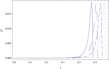
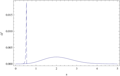
Figure 4: Left: The probability density function $\Omega^{2}$ in (102) versus scale factor $a$. The figure is plotted for different values of the minisuperspace prob energy $E=0.25$, $E=0.5$, $E=0.75$ and $E=1$ from left to right. Right: The comparison of $\Omega^{2}-a$ for two difference cases: FRW metric (solid curve) and rainbow metric (small dashed curve). We also set the numerical values $n=2$, $\lambda=10$, $\phi=5$ and $E_{Pl}=1$.

Figure 4 (left) reflects the fact that in the context of Bohmian quantum mechanics it is possible for our current universe (with initial rainbow FRW metric) to appear from a non-zero value of scale factor. This figure shows that as the energy of prob particles (in particular photons) increases, the peak of $\Omega^{2}$ moves towards greater scale factor. Noting that in limit $E_{Pl}\rightarrow\infty$ the rainbow FRW metric is converted to standard FRW metric, a comparison of these two cases is also plotted in figure 4 (right) from which we see that the peak of $\Omega^{2}$ in FRW background emerges in a larger scale factor in comparison with its rainbow counterpart. However, in rainbow background the probability of the emergence of the universe from a non-zero value scale factor is greater and its corresponding $\Omega^{2}$ is sharper and more localized.

6 Summary and conclusions

In this paper we have investigated the classical and quantum dynamics of a scalar-rainbow metric cosmological model coupled to a perfect fluid in the context of the Schutz’ representation. By means of the Schutz’ formalism for perfect fluid we are able to introduce the only remaining matter degree of freedom as a time parameter in the model. Due to the rainbow FRW background this result has released via a particular energy-dependent gauge fixing. In terms of this time parameter, and in the framework of the Hamiltonian formalism, we have obtained the corresponding classical cosmology by evaluating the dynamical behavior of the cosmic scale factor and the scalar field. We have seen that the classical evolution of the universe, with the rainbow geometry background, represents a late time expansion coming from a big-bang singularity. This is while that if the average prob energy of minisuperspace remains almost constant, there may be possibility of an early bounce (rather than big-bang) from a non-zero value of scale factor. This outcome is interesting from the cosmological standpoint in the sense that based on a classical picture a late time expansion does not come from an initial singularity. We then dealt with the quantization of the model in which we saw that the classical singular behavior will be modified. In the quantum model, we showed that the SWD equation in the presence of rainbow FRW metric can be separated and its eigenfunctions can be obtained in terms of analytical functions. In this regards, the wave functions (81) and (90) are achieved based on two different assumptions on minisuperspace prob energy. Generally, both the wave functions display patterns in which there are two possible quantum states from which our current universe could have evolved and tunneled in the past from one state to another. The wave function (81) has been derived with the assumption that the average prob energy of minisuperspace remains almost constant. Time evolution pattern of this wave function in figure 3 demonstrated that it moves along the larger $a$-direction whereas the scalar field $\phi$ remains constant and does not change its shape. As time passes, our results indicated that the wave packets disperse and the minimum width being attained at $T=0$, which means that the quantum effects are important for small enough $T$, corresponding to small $a$. The wave function (90), on the other hand, has been obtained with this idea that the minisuperspace prob energy does not stays constant. The avoidance of classical singularities due to quantum effects, and the recovery of the classical dynamics of the universe are another important topics of our quantum presentation of the model from which the time evolution of the expectation values of scale factor and scalar field along with their Bohmian counterparts have been assessed. We verified that a bouncing singularity-free universe is obtained in both cases. Finally, by analyzing the probability density function $\Omega^{2}$ versus scale factor $a$ we found that in the rainbow geometric background the probability of the emergence of the universe from a non-zero scale factor is greater than its FRW metric counterpart.

References

- [1] G. Amelino-Camelia, Phys. Lett. B 510, 255 (2001).
- [2] G. Amelino-Camelia, Int. J. Mod. Phys. D 11, 35 (2002).
- [3] G. Amelino-Camelia, J. Kowalski-Glikman, G. Mandanici and A. Procaccini,Int. J. Mod. Phys. A 20, 6007 (2005).
- [4] G. Amelino-Camelia, [arXiv:0309054 [gr-qc]] (2003).
- [5] J. Kowalski-Glikman, Lect. Notes Phys. 669, 131, (2005).
- [6] J. Magueijo and L. Smolin, Phys. Rev. Lett. 88, 190403 (2002).
- [7] J. Magueijo and L. Smolin, Phys. Rev. D 67, 044017 (2003).
- [8] J. Hackett, Class. Quant. Grav. 23, 3833 (2006).
- [9] R. C. Myers and M. Pospelov, Phys. Rev. Lett. 90, 211601 (2003).
- [10] T. Jacobson, S. Liberati and D. Mattingly, Phys. Rev. D 66, 081302 (2002).
- [11] G. Amelino-Camelia and T. Piran, Phys. Rev. D 64, 036005 (2001).
- [12] S. R. Coleman and S. L. Glashow, Phys. Rev. D 59, 116008 (1999).
- [13] N. Hayashida, K. Honda, N. Inoue et. al. Astrophys. J. 522, 255 (1999).
- [14] J. Magueijo and L. Smolin, Class. Quant. Grav. 21, 1725 (2004).
- [15] R. Garattini and E. N. Saridakis, Eur. Phys. J. C 75, 7 343 (2015).
- [16] A. Farag Ali, M. Faizal, M. M. Khalil, Nucl. Phys. B 894, 341 (2015).
- [17] M. Khodadi, Y. Heydarzade, K. Nozari, F. Darabi, Eur. Phys. J. C 75, 12 590 (2015).
- [18] S. H. Hendi, M. Faizal, Phys. Rev. D 92 4, 044027 (2015).
- [19] Y. Gim, W. Kim, JCAP, 10, 003 (2014).
- [20] A. F. Ali, Phys. Rev. D 89, 104040 (2014).
- [21] J. D. Barrow, J. Magueijo, Phys. Rev. D 88, 10 103525 (2013).
- [22] G. Amelino-Camelia, M. Arzano, G. Gubitosi, J. Magueijo, Phys. Rev. D 88, 041303, (2013).
- [23] R. Garattini, JCAP 1306, 017 (2013).
- [24] A. Awad, A. F. Ali, B. Majumder, JCAP 10, 052 (2013).
- [25] Y. Ling, Q. Wu, Phys. Lett. B 687, 103 (2010).
- [26] S. H. Hendi, S. Panahiyan, B. Eslam Panah and M. Momennia, Eur. Phys. J. C 76, 150 (2016).
- [27] Y. Ling, JCAP 0708, 017 (2007).
- [28] B. Vakili, Phys. Lett. B 688, 129 (2010).
- [29] B. F. Schutz, Phys. Rev. D 2, 2762 (1970).
- [30] B. F. Schutz, Phys. Rev. D 4, 3559 (1971).
- [31] B. Majumder, Int. J. Mod. Phys. D, 22, 1350079 (2013).
- [32] F. G. Alvarenga, J. C. Fabris, N. A. Lemos and G. A. Monerat, Gen. Rel. Grav. 34, 651 (2002).
- [33] M. Khodadi, K. Nozari, H. R. Sepangi, [arXiv:1602.02921 [gr-qc]] (2016).
- [34] F. G. Alvarenga , A. B. Batista, J. C. Fabris and S. V. B. Goncalves, Gen. Rel. Grav. 35, 1659 (2003).
- [35] R. Garattini and G. Mandanici, Phys. Rev. D 83, 084021 (2011).
- [36] S. W. Hawking and G. F. R. Ellis, The Large Strucure of Space-Time, Cambridge University Press, 1973
- [37] V. G. Lapchinski and V. A. Rubakov, Theor. Math. Phys. 33, 1076 (1977).
- [38] A. Awad, Phys. Rev. D 87, 103001 (2013).
- [39] M. Abramowitz and I. A. Stegun, Handbook of Mathematical Functions, New York: Dover (1972).
- [40] F. J. Tipler, Phys. Rep. 137, 231 (1986).