Learning Global Features for Coreference Resolution

Abstract

There is compelling evidence that coreference prediction would benefit from modeling global information about entity-clusters. Yet, state-of-the-art performance can be achieved with systems treating each mention prediction independently, which we attribute to the inherent difficulty of crafting informative cluster-level features. We instead propose to use recurrent neural networks (RNNs) to learn latent, global representations of entity clusters directly from their mentions. We show that such representations are especially useful for the prediction of pronominal mentions, and can be incorporated into an end-to-end coreference system that outperforms the state of the art without requiring any additional search.

1 Introduction

While structured, non-local coreference models would seem to hold promise for avoiding many common coreference errors (as discussed further in Section 3), the results of employing such models in practice are decidedly mixed, and state-of-the-art results can be obtained using a completely local, mention-ranking system.

In this work, we posit that global context is indeed necessary for further improvements in coreference resolution, but argue that informative cluster, rather than mention, level features are very difficult to devise, limiting their effectiveness. Accordingly, we instead propose to learn representations of mention clusters by embedding them sequentially using a recurrent neural network (shown in Section 4). Our model has no manually defined cluster features, but instead learns a global representation from the individual mentions present in each cluster. We incorporate these representations into a mention-ranking style coreference system.

The entire model, including the recurrent neural network and the mention-ranking sub-system, is trained end-to-end on the coreference task. We train the model as a local classifier with fixed context (that is, as a history-based model). As such, unlike several recent approaches, which may require complicated inference during training, we are able to train our model in much the same way as a vanilla mention-ranking model.

Experiments compare the use of learned global features to several strong baseline systems for coreference resolution. We demonstrate that the learned global representations capture important underlying information that can help resolve difficult pronominal mentions, which remain a persistent source of errors for modern coreference systems [Durrett and Klein (2013, Kummerfeld and Klein (2013, Wiseman et al. (2015, Martschat and Strube (2015]. Our final system improves over 0.8 points in CoNLL score over the current state of the art, and the improvement is statistically significant on all three CoNLL metrics.

2 Background and Notation

Coreference resolution is fundamentally a clustering task. Given a sequence $(x_{n})_{n=1}^{N}$ of (intra-document) mentions – that is, syntactic units that can refer or be referred to – coreference resolution involves partitioning $(x_{n})$ into a sequence of clusters $(X^{(m)})_{m=1}^{M}$ such that all the mentions in any particular cluster $X^{(m)}$ refer to the same underlying entity. Since the mentions within a particular cluster may be ordered linearly by their appearance in the document, we will use the notation $X_{j}^{(m)}$ to refer to the $j$’th mention in the $m$’th cluster.

A valid clustering places each mention in exactly one cluster, and so we may represent a clustering with a vector $\boldsymbol{z}\,{\in}\,\{1,\ldots,M\}^{N}$, where $z_{n}\,{=}\,m$ iff $x_{n}$ is a member of $X^{(m)}$. Coreference systems attempt to find the best clustering $\boldsymbol{z}^{*}\in\mathcal{Z}$ under some scoring function, with $\mathcal{Z}$ the set of valid clusterings.

One strategy to avoid the computational intractability associated with predicting an entire clustering $\boldsymbol{z}$ is to instead predict a single antecedent for each mention $x_{n}$; because $x_{n}$ may not be anaphoric (and therefore have no antecedents), a “dummy” antecedent $\epsilon$ may also be predicted. The aforementioned strategy is adopted by “mention-ranking” systems [Denis and Baldridge (2008, Rahman and Ng (2009, Durrett and Klein (2013], which, formally, predict an antecedent $\hat{y}\,{\in}\,\mathcal{Y}(x_{n})$ for each mention $x_{n}$, where $\mathcal{Y}(x_{n})\,{=}\,\{1,\ldots,n-1,\epsilon\}$. Through transitivity, these decisions induce a clustering over the document.

Mention-ranking systems make their antecedent predictions with a local scoring function $f(x_{n},y)$ defined for any mention $x_{n}$ and any antecedent $y\,{\in}\,\mathcal{Y}(x_{n})$. While such a scoring function clearly ignores much structural information, the mention-ranking approach has been attractive for at least two reasons. First, inference is relatively simple and efficient, requiring only a left-to-right pass through a document’s mentions during which a mention’s antecedents (as well as $\epsilon$) are scored and the highest scoring antecedent is predicted. Second, from a linguistic modeling perspective, mention-ranking models learn a scoring function that requires a mention $x_{n}$ to be compatible with only one of its coreferent antecedents. This contrasts with mention-pair models (e.g., ?)), which score all pairs of mentions in a cluster, as well as with certain cluster-based models (see discussion in ?)). Modeling each mention as having a single antecedent is particularly advantageous for pronominal mentions, which we might like to model as linking to a single nominal or proper antecedent, for example, but not necessarily to all other coreferent mentions.

Accordingly, in this paper we attempt to maintain the inferential simplicity and modeling benefits of mention ranking, while allowing the model to utilize global, structural information relating to $\boldsymbol{z}$ in making its predictions. We therefore investigate objective functions of the form

$$\operatornamewithlimits{arg\,max}_{y_{1},\ldots,y_{N}}\sum_{n=1}^{N}f(x_{n},y_{n})+g(x_{n},y_{n},\boldsymbol{z}_{1:n-1}){\makebox[0.0pt][l]{\qquad\rm{,}}}$$

where $g$ is a global function that, in making predictions for $x_{n}$, may examine (features of) the clustering $\boldsymbol{z}_{1:n-1}$ induced by the antecedent predictions made through $y_{n-1}$.

3 The Role of Global Features

Here we motivate the use of global features for coreference resolution by focusing on the issues that may arise when resolving pronominal mentions in a purely local way. See ?) and ?) for more general motivation for using global models.

3.1 Pronoun Problems

Recent empirical work has shown that the resolution of pronominal mentions accounts for a substantial percentage of the total errors made by modern mention-ranking systems. ?) show that on the CoNLL 2012 English development set, almost 59% of mention-ranking precision errors and almost 24% of recall errors involve pronominal mentions. ?) found a similar pattern in their comparison of mention-ranking, mention-pair, and latent-tree models.

To see why pronouns can be so problematic, consider the following passage from the “Broadcast Conversation” portion of the CoNLL development set (bc/msnbc/0000/018); below, we enclose mentions in brackets and give the same subscript to co-clustered mentions. (This example is also shown in Figure 2.)

DA: um and [I]₁ think that is what’s - Go ahead [Linda]₂.

LW: Well and uh thanks goes to [you]₁ and to [the media]₃ to help [us]₄…So [our]₄ hat is off to all of [you]₅ as well.

This example is typical of Broadcast Conversation, and it is difficult because local systems learn to myopically link pronouns such as [you]₅ to other instances of the same pronoun that are close by, such as [you]₁. While this is often a reasonable strategy, in this case predicting [you]₁ to be an antecedent of [you]₅ would result in the prediction of an incoherent cluster, since [you]₁ is coreferent with the singular [I]₁, and [you]₅, as part of the phrase “all of you,” is evidently plural. Thus, while there is enough information in the text to correctly predict [you]₅, doing so crucially depends on having access to the history of predictions made so far, and it is precisely this access to history that local models lack.

More empirically, there are non-local statistical regularities involving pronouns we might hope models could exploit. For instance, in the CoNLL training data over 70% of pleonastic “it” instances and over 74% of pleonastic “you” instances follow (respectively) previous pleonastic “it” and “you” instances. Similarly, over 78% of referential “I” instances and over 68% of referential “he” instances corefer with previous “I” and “he” instances, respectively.

Accordingly, we might expect non-local models with access to global features to perform significantly better. However, models incorporating non-local features have a rather mixed track record. For instance, ?) found that cluster-level features improved their results, whereas ?) found that they did not. ?) found that incorporating cluster-level features beyond those involving the pre-computed mention-pair and mention-ranking probabilities that form the basis of their agglomerative clustering coreference system did not improve performance. Furthermore, among recent, state-of-the-art systems, mention-ranking systems (which are completely local) perform at least as well as their more structured counterparts [Durrett and Klein (2014, Clark and Manning (2015, Wiseman et al. (2015, Peng et al. (2015].

3.2 Issues with Global Features

We believe a major reason for the relative ineffectiveness of global features in coreference problems is that, as noted by ?), cluster-level features can be hard to define. Specifically, it is difficult to define discrete, fixed-length features on clusters, which can be of variable size (or shape). As a result, global coreference features tend to be either too coarse or too sparse. Thus, early attempts at defining cluster-level features simply applied the coarse quantifier predicates all, none, most to the mention-level features defined on the mentions (or pairs of mentions) in a cluster [Culotta et al. (2007, Rahman and Ng (2011]. For example, a cluster would have the feature ‘most-female=true’ if more than half the mentions (or pairs of mentions) in the cluster have a ‘female=true’ feature.

On the other extreme, ?) define certain cluster-level features by concatenating the mention-level features of a cluster’s constituent mentions in order of the mentions’ appearance in the document. For example, if a cluster consists, in order, of the mentions (the president, he, he), they would define a cluster-level “type” feature ‘C-P-P=true’, which indicates that the cluster is composed, in order, of a common noun, a pronoun, and a pronoun. While very expressive, these concatenated features are often quite sparse, since clusters encountered during training can be of any size.

4 Learning Global Features

To circumvent the aforementioned issues with defining global features, we propose to learn cluster-level feature representations implicitly, by identifying the state of a (partial) cluster with the hidden state of an RNN that has consumed the sequence of mentions composing the (partial) cluster. Before providing technical details, we provide some preliminary evidence that such learned representations capture important contextual information by displaying in Figure 1 the learned final states of all clusters in the CoNLL development set, projected using T-SNE [van der Maaten and Hinton (2012]. Each point in the visualization represents the learned features for an entity cluster and the head words of mentions are shown for representative points. Note that the model learns to roughly separate clusters by simple distinctions such as predominant type (nominal, proper, pronominal) and number (it, they, etc), but also captures more subtle relationships such as grouping geographic terms and long strings of pronouns.

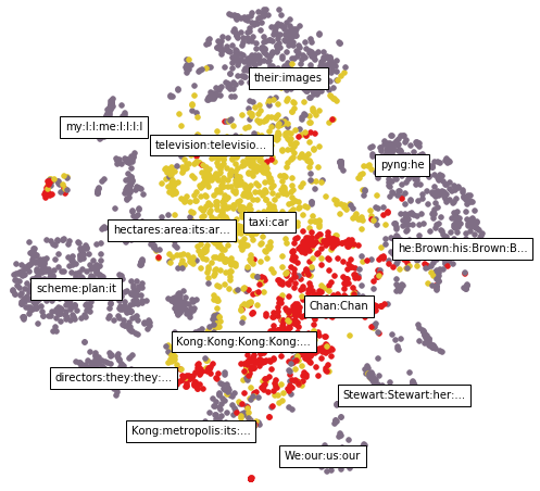
Figure 1: T-SNE visualization of learned entity representations on the CoNLL development set. Each point shows a gold cluster of size $>$ 1. Yellow, red, and purple points represent predominantly common noun, proper noun, and pronoun clusters, respectively. Captions show head words of representative clusters’ mentions.

4.1 Recurrent Neural Networks

A recurrent neural network is a parameterized non-linear function $\mathrm{\mathbf{RNN}}$ that recursively maps an input sequence of vectors to a sequence of hidden states. Let $(\boldsymbol{m}_{j})_{j=1}^{J}$ be a sequence of $J$ input vectors $\boldsymbol{m}_{j}\,{\in}\,\mathbb{R}^{D}$, and let $\boldsymbol{h}_{0}\,{=}\,\mathbf{0}$. Applying an RNN to any such sequence yields

$$\boldsymbol{h}_{j}\leftarrow\mathrm{\mathbf{RNN}}(\boldsymbol{m}_{j},\boldsymbol{h}_{j-1};\boldsymbol{\theta}){\makebox[0.0pt][l]{\qquad\rm{,}}}$$

where $\boldsymbol{\theta}$ is the set of parameters for the model, which are shared over time.

There are several varieties of RNN, but by far the most commonly used in natural-language processing is the Long Short-Term Memory network (LSTM) [Hochreiter and Schmidhuber (1997], particularly for language modeling (e.g., ?)) and machine translation (e.g., ?)), and we use LSTMs in all experiments.

DA: um and [I]₁ think that is what’s - Go ahead [Linda]₂.

LW: Well and thanks goes to [you]₁ and to [the media]₃ to help [us]₄…So [our]₄ hat is off to all of [you]₅…

Figure 2: Full RNN example for handling the mention $x_{n}=$ [you]. There are currently four entity clusters in scope $X^{(1)},X^{(2)},X^{(3)},X^{(4)}$ based on unseen previous decisions $(y)$. Each cluster has a corresponding RNN state, two of which ($\boldsymbol{h}^{(1)}$ and $\boldsymbol{h}^{(4)}$) have processed multiple mentions (with $X^{(1)}$ notably including a singular mention [I]). At the bottom, we show the complete mention-ranking process. Each previous mention is considered as an antecedent, and the global term considers the antecedent clusters’ current hidden state. Selecting $\epsilon$ is treated with a special case $\mathrm{NA}(x_{n})$.

4.2 RNNs for Cluster Features

Our main contribution will be to utilize RNNs to produce feature representations of entity clusters which will provide the basis of the global term $g$. Recall that we view a cluster $X^{(m)}$ as a sequence of mentions $(X^{(m)}_{j})_{j=1}^{J}$ (ordered in linear document order). We therefore propose to embed the state(s) of $X^{(m)}$ by running an RNN over the cluster in order.

In order to run an RNN over the mentions we need an embedding function $\boldsymbol{h}_{\mathrm{c}}$ to map a mention to a real vector. First, following ?) define $\boldsymbol{\phi}_{\mathrm{a}}(x_{n}):\mathcal{X}\rightarrow\{0,1\}^{F}$ as a standard set of local indicator features on a mention, such as its head word, its gender, and so on. (We elaborate on features below.) We then use a non-linear feature embedding $\boldsymbol{h}_{\mathrm{c}}$ to map a mention $x_{n}$ to a vector-space representation. In particular, we define

$$\boldsymbol{h}_{\mathrm{c}}(x_{n}) \triangleq\tanh(\boldsymbol{W}_{\mathrm{\mathrm{c}}}\,\boldsymbol{\phi}_{\mathrm{a}}(x_{n})+\boldsymbol{b}_{\mathrm{\mathrm{c}}}){\makebox[0.0pt][l]{\qquad\rm{,}}}$$

where $\boldsymbol{W}_{\mathrm{\mathrm{c}}}$ and $\boldsymbol{b}_{\mathrm{\mathrm{c}}}$ are parameters of the embedding.

We will refer to the $j$’th hidden state of the RNN corresponding to $X^{(m)}$ as $\boldsymbol{h}^{(m)}_{j}$, and we obtain it according to the following formula

$$\boldsymbol{h}^{(m)}_{j}\leftarrow\mathrm{\mathbf{RNN}}(\boldsymbol{h}_{\mathrm{c}}(X_{j}^{(m)}),\boldsymbol{h}^{(m)}_{j-1};\boldsymbol{\theta}){\makebox[0.0pt][l]{\qquad\rm{,}}}$$

again assuming that $\boldsymbol{h}^{(m)}_{0}\,{=}\,\boldsymbol{0}$. Thus, we will effectively run an RNN over each (sequence of mentions corresponding to a) cluster $X^{(m)}$ in the document, and thereby generate a hidden state $\boldsymbol{h}^{(m)}_{j}$ corresponding to each step of each cluster in the document. Concretely, this can be implemented by maintaining $M$ RNNs – one for each cluster – that all share the parameters $\boldsymbol{\theta}$. The process is illustrated in the top portion of Figure 2.

5 Coreference with Global Features

We now describe how the RNN defined above is used within an end-to-end coreference system.

5.1 Full Model and Training

Recall that our inference objective is to maximize the score of both a local mention ranking term as well as a global term based on the current clusters:

$$\operatornamewithlimits{arg\,max}_{y_{1},\ldots,y_{N}}\sum_{n=1}^{N}f(x_{n},y_{n})+g(x_{n},y_{n},\boldsymbol{z}_{1:n-1})$$

We begin by defining the local model $f(x_{n},y)$ with the two layer neural network of ?), which has a specialization for the non-anaphoric case, as follows:

$$f(x_{n},y) \triangleq\begin{cases}\boldsymbol{u}^{\mathsf{T}}\left[\begin{smallmatrix}\boldsymbol{h}_{\mathrm{a}}(x_{n})\\ \boldsymbol{h}_{\mathrm{p}}(x_{n},y)\end{smallmatrix}\right]+u_{0}&\mbox{if }y\neq\epsilon\\ \boldsymbol{v}^{\mathsf{T}}\boldsymbol{h}_{\mathrm{a}}(x_{n})+v_{0}&\mbox{if }y=\epsilon{\makebox[0.0pt][l]{\qquad\rm{.}}}\end{cases}$$

Above, $\boldsymbol{u}$ and $\boldsymbol{v}$ are the parameters of the model, and $\boldsymbol{h}_{\mathrm{a}}$ and $\boldsymbol{h}_{\mathrm{p}}$ are learned feature embeddings of the local mention context and the pairwise affinity between a mention and an antecedent, respectively. These feature embeddings are defined similarly to $\boldsymbol{h}_{\mathrm{c}}$, as

$$\boldsymbol{h}_{\mathrm{a}}(x_{n}) \triangleq\tanh(\boldsymbol{W}_{\mathrm{\mathrm{a}}}\,\boldsymbol{\phi}_{\mathrm{a}}(x_{n})+\boldsymbol{b}_{\mathrm{\mathrm{a}}})$$

$$\boldsymbol{h}_{\mathrm{p}}(x_{n},y) \triangleq\tanh(\boldsymbol{W}_{\mathrm{\mathrm{p}}}\,\boldsymbol{\phi}_{\mathrm{p}}(x_{n},y)+\boldsymbol{b}_{\mathrm{\mathrm{p}}}){\makebox[0.0pt][l]{\qquad\rm{,}}}$$

where $\boldsymbol{\phi}_{\mathrm{a}}$ (mentioned above) and $\boldsymbol{\phi}_{\mathrm{p}}$ are “raw” (that is, unconjoined) features on the context of $x_{n}$ and on the pairwise affinity between mentions $x_{n}$ and antecedent $y$, respectively [Wiseman et al. (2015]. Note that $\boldsymbol{h}_{\mathrm{a}}$ and $\boldsymbol{h}_{\mathrm{c}}$ use the same raw features; only their weights differ.

We now specify our global scoring function $g$ based on the history of previous decisions. Define $\boldsymbol{h}_{<n}^{(m)}$ as the hidden state of cluster $m$ before a decision is made for $x_{n}$ – that is, $\boldsymbol{h}_{<n}^{(m)}$ is the state of cluster $m$’s RNN after it has consumed all mentions in the cluster preceding $x_{n}$. We define $g$ as

$$g(x_{n},y, \boldsymbol{z}_{1:n-1}) \triangleq\begin{cases}\boldsymbol{h}_{\mathrm{c}}(x_{n})^{\mathsf{T}}\boldsymbol{h}^{(z_{y})}_{<n}&\mbox{if }y\neq\epsilon\\ \mathrm{NA}(x_{n})&\mbox{if }y=\epsilon{\makebox[0.0pt][l]{\qquad\rm{,}}}\end{cases}$$

where $\mathrm{NA}$ gives a score for assigning $\epsilon$ based on a non-linear function of all of the current hidden states:

$$\mathrm{NA}(x_{n})=\boldsymbol{q}^{\mathsf{T}}\tanh\left(\boldsymbol{W}_{s}\left[\begin{smallmatrix}\boldsymbol{\phi}_{\mathrm{a}}(x_{n})\\ \sum_{m=1}^{M}\boldsymbol{h}^{(m)}_{<n}\end{smallmatrix}\right]+\boldsymbol{b}_{s}\right).$$

See Figure 2 for a diagram. The intuition behind the first case in $g$ is that in considering whether $y$ is a good antecedent for $x_{n}$, we add a term to the score that examines how well $x_{n}$ matches with the mentions already in $X^{(z_{y})}$; this matching score is expressed via a dot-product. In the second case, when predicting that $x_{n}$ is non-anaphoric, we add the NA term to the score, which examines the (sum of) the current states $\boldsymbol{h}^{(m)}_{<n}$ of all clusters. This information is useful both because it allows the non-anaphoric score to incorporate information about potential antecedents, and because the occurrence of certain singleton-clusters often predicts the occurrence of future singleton-clusters, as noted in Section 3.

The whole system is trained end-to-end on coreference using backpropagation. For a given training document, let $\boldsymbol{z}^{(o)}$ be the oracle mapping from mention to cluster, which induces an oracle clustering. While at training time we do have oracle clusters, we do not have oracle antecedents $(y)_{n=1}^{N}$, so following past work we treat the oracle antecedent as latent [Yu and Joachims (2009, Fernandes et al. (2012, Chang et al. (2013, Durrett and Klein (2013]. We train with the following slack-rescaled, margin objective:

$$\sum_{n=1}^{N}\max_{\hat{y}\in\mathcal{Y}(x_{n})}\Delta(x_{n},\hat{y}) (1+f(x_{n},\hat{y})+g(x_{n},\hat{y},\boldsymbol{z}^{(o)})$$

$$-f(x_{n},y_{n}^{\ell})-g(x_{n},y_{n}^{\ell},\boldsymbol{z}^{(o)})),$$

where the latent antecedent $y_{n}^{\ell}$ is defined as

$$\small y_{n}^{\ell}\triangleq\operatornamewithlimits{arg\,max}_{y\in\mathcal{Y}(x_{n}):z^{(o)}_{y}=z^{(o)}_{n}}f(x_{n},y)+g(x_{n},y,\boldsymbol{z}^{(o)})$$

if $x_{n}$ is anaphoric, and is $\epsilon$ otherwise. The term $\Delta(x_{n},\hat{y})$ gives different weight to different error types. We use a $\Delta$ with 3 different weights $(\alpha_{1},\alpha_{2},\alpha_{3})$ for “false link” (fl), “false new” (fn), and “wrong link” (wl) mistakes [Durrett and Klein (2013], which correspond to predicting an antecedent when non-anaphoric, $\epsilon$ when anaphoric, and the wrong antecedent, respectively.

Note that in training we use the oracle clusters $\boldsymbol{z}^{(o)}$. Since these are known a priori, we can pre-compute all the hidden states $\boldsymbol{h}_{j}^{(m)}$ in a document, which makes training quite simple and efficient. This approach contrasts in particular with the work of ?) — who also incorporate global information in mention-ranking — in that they train against latent trees, which are not annotated and must be searched for during training. On the other hand, training on oracle clusters leads to a mismatch between training and test, which can hurt performance.

5.2 Search

When moving from a strictly local objective to one with global features, the test-time search problem becomes intractable. The local objective requires $O(n^{2})$ time, whereas the full clustering problem is NP-Hard. Past work with global features has used integer linear programming solvers for exact search [Chang et al. (2013, Peng et al. (2015], or beam search with (delayed) early update training for an approximate solution [Björkelund and Kuhn (2014]. In contrast, we simply use greedy search at test time, which also requires $O(n^{2})$ time. The full algorithm is shown in Algorithm 1. The greedy search algorithm is identical to a simple mention-ranking system, with the exception of line 11, which updates the current RNN representation based on the previous decision that was made, and line 4, which then uses this cluster representation as part of scoring.

1:procedure GreedyCluster($x_{1},\ldots,x_{N}$)

2:    Initialize clusters $X^{(1)}\ldots$ as empty lists, hidden states $\boldsymbol{h}^{(0)},\ldots$ as $\mathbf{0}$ vectors in $\mathbb{R}^{D}$, $\boldsymbol{z}$ as map from mention to cluster, and cluster counter $M\leftarrow 0$

3:    for $n=2\ldots N$  do

4:        $\displaystyle y^{*}\leftarrow\operatornamewithlimits{arg\,max}_{y\in\mathcal{Y}(x_{n})}f(x_{n},y)+g(x_{n},y,\boldsymbol{z}_{1:n-1})$

5:        $m\leftarrow z_{y^{*}}$

6:        if $y^{*}=\epsilon$ then

7:           $M\leftarrow M+1$

8:           $m\leftarrow M$         

9:        append $x_{n}$ to $X^{(m)}$

10:        $z_{n}\leftarrow m$

11:        $\boldsymbol{h}^{(m)}\leftarrow\mathrm{\mathbf{RNN}}(\boldsymbol{h}_{\mathrm{c}}(x_{n}),\boldsymbol{h}^{(m)})$     

12:    return $X^{(1)},\ldots,X^{(M)}$

Algorithm 1 Greedy search with global RNNs

6 Experiments

6.1 Methods

System	MUC			B3			CEAFe
	P	R	F1	P	R	F1	P	R	F1	CoNLL
B&K (2014)	74.30	67.46	70.72	62.71	54.96	58.58	59.40	52.27	55.61	61.63
M&S (2015)	76.72	68.13	72.17	66.12	54.22	59.58	59.47	52.33	55.67	62.47
C&M (2015)	76.12	69.38	72.59	65.64	56.01	60.44	59.44	52.98	56.02	63.02
Peng et al. (2015)	-	-	72.22	-	-	60.50	-	-	56.37	63.03
Wiseman et al. (2015)	76.23	69.31	72.60	66.07	55.83	60.52	59.41	54.88	57.05	63.39
This work	77.49	69.75	73.42	66.83	56.95	61.50	62.14	53.85	57.70	64.21

Table 1: Results on CoNLL 2012 English test set. We compare against recent state of the art systems, including (in order) Bjorkelund and Kuhn (2014), Martschat and Strube (2015), Clark and Manning (2015), Peng et al. (2015), and Wiseman et al. (2015). F₁ gains are significant ($p<0.05$ under the bootstrap resample test (Koehn, 2004)) compared with Wiseman et al. (2015) for all metrics.

We run experiments on the CoNLL 2012 English shared task [Pradhan et al. (2012]. The task uses the OntoNotes corpus [Hovy et al. (2006], consisting of 3,493 documents in various domains and formats. We use the experimental split provided in the shared task. For all experiments, we use the Berkeley Coreference System [Durrett and Klein (2013] for mention extraction and to compute features $\boldsymbol{\phi}_{\mathrm{a}}$ and $\boldsymbol{\phi}_{\mathrm{p}}$.

Features

We use the raw Basic+ feature sets described by ?), with the following modifications:

• We remove all features from $\boldsymbol{\phi}_{\mathrm{p}}$ that concatenate a feature of the antecedent with a feature of the current mention, such as bi-head features.

• We add true-cased head features, a current speaker indicator feature, and a 2-character genre (out of {bc,bn,mz,nw,pt,tc,wb}) indicator to $\boldsymbol{\phi}_{\mathrm{p}}$ and $\boldsymbol{\phi}_{\mathrm{a}}$.

• We add features indicating if a mention has a substring overlap with the current speaker ($\boldsymbol{\phi}_{\mathrm{p}}$ and $\boldsymbol{\phi}_{\mathrm{a}}$), and if an antecedent has a substring overlap with a speaker distinct from the current mention’s speaker ($\boldsymbol{\phi}_{\mathrm{p}}$).

• We add a single centered, rescaled document position feature to each mention when learning $\boldsymbol{h}_{\mathrm{c}}$. We calculate a mention $x_{n}$’s rescaled document position as $\frac{2n-N-1}{N-1}$.

These modifications result in there being approximately 14K distinct features in $\boldsymbol{\phi}_{\mathrm{a}}$ and approximately 28K distinct features in $\boldsymbol{\phi}_{\mathrm{p}}$, which is far fewer features than has been typical in past work.

For training, we use document-size minibatches, which allows for efficient pre-computation of RNN states, and we minimize the loss described in Section 5 with AdaGrad [Duchi et al. (2011] (after clipping LSTM gradients to lie (elementwise) in $(-10,10)$). We find that the initial learning rate chosen for AdaGrad has a significant impact on results, and we choose learning rates for each layer out of $\{0.1,0.02,0.01,0.002,0.001\}$.

In experiments, we set $\boldsymbol{h}_{\mathrm{a}}(x_{n})$, $\boldsymbol{h}_{\mathrm{c}}(x_{n})$, and $\boldsymbol{h}^{(m)}$ to be $\,{\in}\,\mathbb{R}^{200}$, and $\boldsymbol{h}_{\mathrm{p}}(x_{n},y)\,{\in}\,\mathbb{R}^{700}$. We use a single-layer LSTM (without “peep-hole” connections), as implemented in the element-rnn library [Léonard et al. (2015]. For regularization, we apply Dropout [Srivastava et al. (2014] with a rate of 0.4 before applying the linear weights $\boldsymbol{u}$, and we also apply Dropout with a rate of 0.3 to the LSTM states before forming the dot-product scores. Following ?) we use the cost-weights $\boldsymbol{\alpha}=\langle 0.5,1.2,1\rangle$ in defining $\Delta$, and we use their pre-training scheme as well. For final results, we train on both training and development portions of the CoNLL data. Scoring uses the official CoNLL 2012 script [Pradhan et al. (2014, Luo et al. (2014]. Code for our system is available at https://github.com/swiseman/nn_coref. The system makes use of a GPU for training, and trains in about two hours.

6.2 Results

	MUC	B3	CEAFe	CoNLL
MR	73.06	62.66	58.98	64.90
Avg, OH	73.30	63.06	58.85	65.07
RNN, GH	73.63	63.23	59.56	65.47
RNN, OH	74.26	63.89	59.54	65.90

Table 2: F₁ scores of models described in text on CoNLL 2012 development set. Rows in grey highlight models using oracle history.

	Non-Anaphoric (fl)
	Nom. HM	Nom. No HM	Pron.
MR	1061	1130	1075
Avg, OH	1983	1140	1011
RNN, GH	1914	1125	1893
RNN, OH	1913	1130	1842
# Mentions	9.0K	22.2K	3.1K
	Anaphoric (fn + wl)
Model	Nom. HM	Nom. No HM	Pron.
MR	665+326	666+56	533+796
Avg, OH	781+300	641+60	578+744
RNN, GH	767+303	648+57	664+727
RNN, OH	750+289	648+52	611+686
# Mentions	4.7K	1.0K	7.3K

Table 3: Number of “false link” (fl) errors on non-anaphoric mentions (top) and number of “false new” (fn) and “wrong link” (wl) errors on anaphoric mentions (bottom) on CoNLL 2012 development set. Mentions are categorized as nominal or proper with (previous) head match (Nom. HM), nominal or proper with no head match (Nom. No HM), and pronominal. Models are described in the text, and rows in grey highlight models using oracle history.

In Table 1 we present our main results on the CoNLL English test set, and compare with other recent state-of-the-art systems. We see a statistically significant improvement of over 0.8 CoNLL points over the previous state of the art, and the highest F₁ scores to date on all three CoNLL metrics.

We now consider in more detail the impact of global features and RNNs on performance. For these experiments, we report MUC, B³, and CEAF_e F₁-scores in Table 2 as well as errors broken down by mention type and by whether the mention is anaphoric or not in Table 3. Table 3 further partitions errors into fl, fn, and wl categories, which are defined in Section 5.1. We typically think of fl and wl as representing precision errors, and fn as representing recall errors.

Our experiments consider several different settings. First, we consider an oracle setting (“RNN, OH” in tables), in which the model receives $\boldsymbol{z}_{1:n-1}^{(o)}$, the oracle partial clustering of all mentions preceding $x_{n}$ in the document, and is therefore not forced to rely on its own past predictions when predicting $x_{n}$. This provides us with an upper bound on the performance achievable with our model. Next, we consider the performance of the model under a greedy inference strategy (RNN, GH), as in Algorithm 1. Finally, for baselines we consider the mention-ranking system (MR) of ?) using our updated feature-set, as well as a non-local baseline with oracle history (Avg, OH), which averages the representations $\boldsymbol{h}_{\mathrm{c}}(x_{j})$ for all $x_{j}\,{\in}\,X^{(m)}$, rather than feed them through an RNN; errors are still backpropagated through the $\boldsymbol{h}_{\mathrm{c}}$ representations during learning.

In Table 3 we see that the RNN improves performance overall, with the most dramatic improvements on non-anaphoric pronouns, though errors are also decreased significantly for non-anaphoric nominal and proper mentions that follow at least one mention with the same head. While wl errors also decrease for both these mention-categories under the RNN model, fn errors increase. Importantly, the RNN performance is significantly better than that of the Avg baseline, which barely improves over mention-ranking, even with oracle history. This suggests that modeling the sequence of mentions in a cluster is advantageous. We also note that while RNN performance degrades in both precision and recall when moving from the oracle history upper-bound to a greedy setting, we are still able to recover a significant portion of the possible performance improvement.

6.3 Qualitative Analysis

In this section we consider in detail the impact of the $g$ term in the RNN scoring function on the two error categories that improve most under the RNN model (as shown in Table 3), namely, pronominal wl errors and pronominal fl errors. We consider an example from the CoNLL development set in each category on which the baseline MR model makes an error but the greedy RNN model does not.

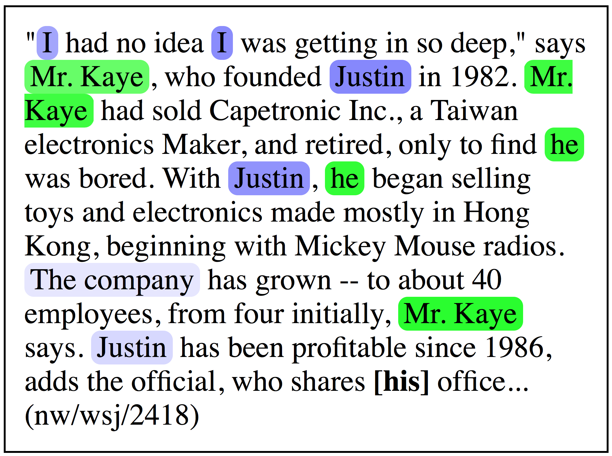
Figure 3: Cluster predictions of greedy RNN model; co-clustered mentions are of the same color, and intensity of mention $x_{j}$ corresponds to $\boldsymbol{h}_{c}(x_{n})^{\mathsf{T}}\boldsymbol{h}_{<k}^{(i)}$, where $k\,{=}\,j+1$, $i\in\{1,2\}$, and $x_{n}=$ “his.” See text for full description.

The example in Figure 3 involves the resolution of the ambiguous pronoun “his,” which is bracketed and in bold in the figure. Whereas the baseline MR model incorrectly predicts “his” to corefer with the closest gender-consistent antecedent “Justin” — thus making a wl error — the greedy RNN model correctly predicts “his” to corefer with “Mr. Kaye” in the previous sentence. (Note that “the official” also refers to Mr. Kaye). To get a sense of the greedy RNN model’s decision-making on this example, we color the mentions the greedy RNN model has predicted to corefer with “Mr. Kaye” in green, and the mentions it has predicted to corefer with “Justin” in blue. (Note that the model incorrectly predicts the initial “I” mentions to corefer with “Justin.”) Letting $X^{(1)}$ refer to the blue cluster, $X^{(2)}$ refer to the green cluster, and $x_{n}$ refer to the ambiguous mention “his,” we further shade each mention $x_{j}$ in $X^{(1)}$ so that its intensity corresponds to $\boldsymbol{h}_{c}(x_{n})^{\mathsf{T}}\boldsymbol{h}_{<k}^{(1)}$, where $k\,{=}\,j+1$; mentions in $X^{(2)}$ are shaded analogously. Thus, the shading shows how highly $g$ scores the compatibility between “his” and a cluster $X^{(i)}$ as each of $X^{(i)}$’s mentions is added. We see that when the initial “Justin” mentions are added to $X^{(1)}$ the $g$-score is relatively high. However, after “The company” is correctly predicted to corefer with “Justin,” the score of $X^{(1)}$ drops, since companies are generally not coreferent with pronouns like “his.”

Figure 4 shows an example (consisting of a telephone conversation between “A” and “B”) in which the bracketed pronoun “It’s” is being used pleonastically. Whereas the baseline MR model predicts “It’s” to corefer with a previous “it” — thus making a fl error — the greedy RNN model does not. In Figure 4 the final mention in three preceding clusters is shaded so its intensity corresponds to the magnitude of the gradient of the $\mathrm{NA}$ term in $g$ with respect to that mention. This visualization resembles the “saliency” technique of ?), and it attempts to gives a sense of the contribution of a (preceding) cluster in the calculation of the $\mathrm{NA}$ score.

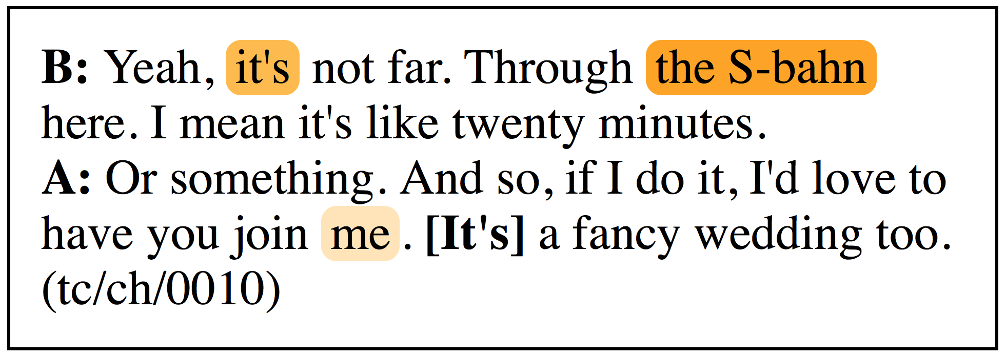
Figure 4: Magnitudes of gradients of $\mathrm{NA}$ score applied to bold “It’s” with respect to final mention in three preceding clusters. See text for full description.

We see that the potential antecedent “S-Bahn” has a large gradient, but also that the initial, obviously pleonastic use of “it’s” has a large gradient, which may suggest that earlier, easier predictions of pleonasm can inform subsequent predictions.

7 Related Work

In addition to the related work noted throughout, we add supplementary references here. Unstructured approaches to coreference typically divide into mention-pair models, which classify (nearly) every pair of mentions in a document as coreferent or not [Soon et al. (2001, Ng and Cardie (2002, Bengtson and Roth (2008], and mention-ranking models, which select a single antecedent for each anaphoric mention [Denis and Baldridge (2008, Rahman and Ng (2009, Durrett and Klein (2013, Chang et al. (2013, Wiseman et al. (2015]. Structured approaches typically divide between those that induce a clustering of mentions [McCallum and Wellner (2003, Culotta et al. (2007, Poon and Domingos (2008, Haghighi and Klein (2010, Stoyanov and Eisner (2012, Cai and Strube (2010], and, more recently, those that learn a latent tree of mentions [Fernandes et al. (2012, Björkelund and Kuhn (2014, Martschat and Strube (2015].

There have also been structured approaches that merge the mention-ranking and mention-pair ideas in some way. For instance, ?) rank clusters rather than mentions; ?) use the output of both mention-ranking and mention pair systems to learn a clustering.

The application of RNNs to modeling (the trajectory of) the state of a cluster is apparently novel, though it bears some similarity to the recent work of ?), who use LSTMs to embed the state of a transition based parser’s stack.

8 Conclusion

We have presented a simple, state of the art approach to incorporating global information in an end-to-end coreference system, which obviates the need to define global features, and moreover allows for simple (greedy) inference. Future work will examine improving recall, and more sophisticated approaches to global training.

References

- [Bengio et al. (2015] Samy Bengio, Oriol Vinyals, Navdeep Jaitly, and Noam Shazeer. 2015. Scheduled sampling for sequence prediction with recurrent neural networks. In Advances in Neural Information Processing Systems, pages 1171–1179.
- [Bengtson and Roth (2008] Eric Bengtson and Dan Roth. 2008. Understanding the Value of Features for Coreference Resolution. In Proceedings of the 2008 Conference on Empirical Methods in Natural Language Processing, pages 294–303. Association for Computational Linguistics.
- [Björkelund and Kuhn (2014] Anders Björkelund and Jonas Kuhn. 2014. Learning structured perceptrons for coreference Resolution with Latent Antecedents and Non-local Features. ACL, Baltimore, MD, USA, June.
- [Cai and Strube (2010] Jie Cai and Michael Strube. 2010. End-to-end coreference resolution via hypergraph partitioning. In 23rd International Conference on Computational Linguistics (COLING), pages 143–151.
- [Chang et al. (2013] Kai-Wei Chang, Rajhans Samdani, and Dan Roth. 2013. A Constrained Latent Variable Model for Coreference Resolution. In Proceedings of the 2013 Conference on Empirical Methods in Natural Language Processing, pages 601–612.
- [Clark and Manning (2015] Kevin Clark and Christopher D. Manning. 2015. Entity-centric coreference resolution with model stacking. In Proceedings of the 53rd Annual Meeting of the Association for Computational Linguistics (ACL), pages 1405–1415.
- [Culotta et al. (2007] Aron Culotta, Michael Wick, Robert Hall, and Andrew McCallum. 2007. First-order Probabilistic Models for Coreference Resolution. In Human Language Technology Conference of the North American Chapter of the Association of Computational Linguistics (NAACL HLT).
- [Daumé III et al. (2009] Hal Daumé III, John Langford, and Daniel Marcu. 2009. Search-based structured prediction. Machine Learning, 75(3):297–325.
- [Denis and Baldridge (2008] Pascal Denis and Jason Baldridge. 2008. Specialized Models and Ranking for Coreference Resolution. In Proceedings of the 2008 Conference on Empirical Methods in Natural Language Processing, pages 660–669. Association for Computational Linguistics.
- [Duchi et al. (2011] John Duchi, Elad Hazan, and Yoram Singer. 2011. Adaptive Subgradient Methods for Online Learning and Stochastic Optimization. The Journal of Machine Learning Research, 12:2121–2159.
- [Durrett and Klein (2013] Greg Durrett and Dan Klein. 2013. Easy Victories and Uphill Battles in Coreference Resolution. In Proceedings of the 2013 Conference on Empirical Methods in Natural Language Processing, pages 1971–1982.
- [Durrett and Klein (2014] Greg Durrett and Dan Klein. 2014. A Joint Model for Entity Analysis: Coreference, Typing, and Linking. Transactions of the Association for Computational Linguistics, 2:477–490.
- [Dyer et al. (2015] Chris Dyer, Miguel Ballesteros, Wang Ling, Austin Matthews, and Noah A. Smith. 2015. Transition-based dependency parsing with stack long short-term memory. In Proceedings of the 53rd Annual Meeting of the Association for Computational Linguistics (ACL), pages 334–343.
- [Fernandes et al. (2012] Eraldo Rezende Fernandes, Cícero Nogueira Dos Santos, and Ruy Luiz Milidiú. 2012. Latent Structure Perceptron with Feature Induction for Unrestricted Coreference Resolution. In Joint Conference on EMNLP and CoNLL-Shared Task, pages 41–48. Association for Computational Linguistics.
- [Haghighi and Klein (2010] Aria Haghighi and Dan Klein. 2010. Coreference Resolution in a Modular, Entity-centered Model. In The 2010 Annual Conference of the North American Chapter of the Association for Computational Linguistics, pages 385–393. Association for Computational Linguistics.
- [Hochreiter and Schmidhuber (1997] Sepp Hochreiter and Jürgen Schmidhuber. 1997. Long short-term memory. Neural Comput., 9:1735–1780.
- [Hovy et al. (2006] Eduard Hovy, Mitchell Marcus, Martha Palmer, Lance Ramshaw, and Ralph Weischedel. 2006. Ontonotes: the 90% Solution. In Proceedings of the human language technology conference of the NAACL, Companion Volume: Short Papers, pages 57–60. Association for Computational Linguistics.
- [Koehn (2004] Philipp Koehn. 2004. Statistical Significance Tests for Machine Translation Evaluation. In Proceedings of the 2004 Conference on Empirical Methods in Natural Language Processing, pages 388–395. Citeseer.
- [Kummerfeld and Klein (2013] Jonathan K. Kummerfeld and Dan Klein. 2013. Error-driven Analysis of Challenges in Coreference Resolution. In Proceedings of the 2013 Conference on Empirical Methods in Natural Language Processing, Seattle, WA, USA, October.
- [Léonard et al. (2015] Nicholas Léonard, Yand Waghmare, Sagar ad Wang, and Jin-Hwa Kim. 2015. rnn: Recurrent Library for Torch. arXiv preprint arXiv:1511.07889.
- [Li et al. (2016] Jiwei Li, Xinlei Chen, Eduard Hovy, and Dan Jurafsky. 2016. Visualizing and understanding neural models in nlp. In NAACL HLT.
- [Luo et al. (2014] Xiaoqiang Luo, Sameer Pradhan, Marta Recasens, and Eduard Hovy. 2014. An Extension of BLANC to System Mentions. Proceedings of ACL, Baltimore, Maryland, June.
- [Martschat and Strube (2015] Sebastian Martschat and Michael Strube. 2015. Latent structures for coreference resolution. TACL, 3:405–418.
- [Martschat et al. (2015] Sebastian Martschat, Thierry Göckel, and Michael Strube. 2015. Analyzing and visualizing coreference resolution errors. In NAACL HLT, pages 6–10.
- [McCallum and Wellner (2003] Andrew McCallum and Ben Wellner. 2003. Toward Conditional Models of Identity Uncertainty with Application to Proper Noun Coreference. Advances in Neural Information Processing Systems 17.
- [Ng and Cardie (2002] Vincent Ng and Claire Cardie. 2002. Identifying Anaphoric and Non-anaphoric Noun Phrases to Improve Coreference Resolution. In Proceedings of the 19th international conference on Computational linguistics-Volume 1, pages 1–7. Association for Computational Linguistics.
- [Peng et al. (2015] Haoruo Peng, Kai-Wei Chang, and Dan Roth. 2015. A joint framework for coreference resolution and mention head detection. In Proceedings of the 19th Conference on Computational Natural Language Learning (CoNLL), pages 12–21.
- [Poon and Domingos (2008] Hoifung Poon and Pedro M. Domingos. 2008. Joint unsupervised coreference resolution with markov logic. In 2008 Conference on Empirical Methods in Natural Language Processing (EMNLP), pages 650–659.
- [Pradhan et al. (2012] Sameer Pradhan, Alessandro Moschitti, Nianwen Xue, Olga Uryupina, and Yuchen Zhang. 2012. Conll-2012 Shared Task: Modeling Multilingual Unrestricted Coreference in OntoNotes. In Joint Conference on EMNLP and CoNLL-Shared Task, pages 1–40. Association for Computational Linguistics.
- [Pradhan et al. (2014] Sameer Pradhan, Xiaoqiang Luo, Marta Recasens, Eduard Hovy, Vincent Ng, and Michael Strube. 2014. Scoring Coreference Partitions of Predicted Mentions: A Reference Implementation. In Proceedings of the Association for Computational Linguistics.
- [Rahman and Ng (2009] Altaf Rahman and Vincent Ng. 2009. Supervised Models for Coreference Resolution. In Proceedings of the 2009 Conference on Empirical Methods in Natural Language Processing: Volume 2-Volume 2, pages 968–977. Association for Computational Linguistics.
- [Rahman and Ng (2011] Altaf Rahman and Vincent Ng. 2011. Narrowing the modeling gap: A cluster-ranking approach to coreference resolution. J. Artif. Intell. Res. (JAIR), 40:469–521.
- [Ross et al. (2011] Stéphane Ross, Geoffrey J. Gordon, and Drew Bagnell. 2011. A reduction of imitation learning and structured prediction to no-regret online learning. In Proceedings of the Fourteenth International Conference on Artificial Intelligence and Statistics, pages 627–635.
- [Soon et al. (2001] Wee Meng Soon, Hwee Tou Ng, and Daniel Chung Yong Lim. 2001. A Machine Learning Approach to Coreference Resolution of Noun Phrases. Computational Linguistics, 27(4):521–544.
- [Srivastava et al. (2014] Nitish Srivastava, Geoffrey Hinton, Alex Krizhevsky, Ilya Sutskever, and Ruslan Salakhutdinov. 2014. Dropout: A simple way to prevent neural networks from overfitting. The Journal of Machine Learning Research, 15(1):1929–1958.
- [Stoyanov and Eisner (2012] Veselin Stoyanov and Jason Eisner. 2012. Easy-first Coreference Resolution. In COLING, pages 2519–2534. Citeseer.
- [Sutskever et al. (2014] Ilya Sutskever, Oriol Vinyals, and Quoc VV Le. 2014. Sequence to sequence learning with neural networks. In Advances in Neural Information Processing Systems (NIPS), pages 3104–3112.
- [van der Maaten and Hinton (2012] Laurens van der Maaten and Geoffrey E. Hinton. 2012. Visualizing non-metric similarities in multiple maps. Machine Learning, 87(1):33–55.
- [Wiseman et al. (2015] Sam Wiseman, Alexander M. Rush, Stuart M. Shieber, and Jason Weston. 2015. Learning anaphoricity and antecedent ranking features for coreference resolution. In Proceedings of the 53rd Annual Meeting of the Association for Computational Linguistics (ACL), pages 1416–1426.
- [Yu and Joachims (2009] Chun-Nam John Yu and Thorsten Joachims. 2009. Learning Structural SVMs with Latent Variables. In Proceedings of the 26th Annual International Conference on Machine Learning, pages 1169–1176. ACM.
- [Zaremba et al. (2014] Wojciech Zaremba, Ilya Sutskever, and Oriol Vinyals. 2014. Recurrent neural network regularization. CoRR, abs/1409.2329.