AC susceptibility as a tool to probe the dipolar interaction in magnetic nanoparticles

Abstract

The dipolar interaction is known to substantially affect the properties of magnetic nanoparticles. This is particularly important when the particles are kept in a fluid suspension or packed inside nano-carriers. In addition to its usual long-range nature, in these cases the dipolar interaction may also induce the formation of clusters of particles, thereby strongly modifying their magnetic anisotropies. In this paper we show how AC susceptibility may be used to obtain important information regarding the influence of the dipolar interaction in a sample. We develop a model which includes both aspects of the dipolar interaction and may be fitted directly to the susceptibility data. The usual long-range nature of the interaction is implemented using a mean-field solution, whereas the particle-particle aggregation is modeled using a distribution of anisotropy constants. The model is then applied to two samples studied at different concentrations. One consists of spherical magnetite nanoparticles dispersed in oil and the other of cubic magnetite nanoparticles embedded on PLGA nanospheres. We also introduce a simple technique to access the importance of the dipolar interaction in a given sample, based on the height of the AC susceptibility peaks for different driving frequencies. Our results help illustrate the important effect that the dipolar interaction has in most nanoparticle samples.

I Introduction

Magnetic nanoparticles (MNPs) have been an active topic of research for over half a century. Initially, much of this interest was related to the magnetic recording industry, but in the past few decades there has been a shift toward biologically inclined applications.Krishnan (2010) Examples include the use of MNPs for drug delivery,Dobson (2006); Nobuto et al. (2004); Babincová et al. (2002) stem cell labeling,Lu et al. (2007); Bulte et al. (2001) water treatments,Yavuz et al. (2006) contrast agents for nuclear magnetic resonanceLarsen et al. (2008) and magnetic hyperthermia. Gilchrist et al. (1957); Hilger and Hergt (2005); Pankhurst et al. (2009); Lee et al. (2011); Branquinho et al. (2013); Andreu et al. (2015a, b); Rodrigues et al. (2013); Dennis et al. (2009); Maier-Hauff et al. (2011) The latter, in particular, is a cancer treatment technique that has already entered clinical trialsMaier-Hauff et al. (2011) and is now considered the most promising application of MNPs. Great progress has also been made in our theoretical understanding of MNPs, particularly through Brown’s Fokker-Planck equation,Brown (1963); *Brown1979a; Coffey et al. (2004) which has allowed us to make valuable predictions about many dynamic properties,Coffey et al. (1993); *Coffey2013; Shliomis and Stepanov (1993); García-Palacios and Lázaro (1998); *Garcia-Palacios2000; Kalmykov and Titov (1999); *Kalmykov2010; Usov and Grebenshchikov (2009a); *Usov2009a; Déjardin et al. (2010); Poperechny et al. (2010); Ouari et al. (2013); Landi (2012a); *Landi2012b; *Landi2012e therefore providing a microscopic platform to describe hyperthermia experiments.Carrey et al. (2011); Verde et al. (2012a); *Verde2012a; *Landi2012f

Most of our theoretical understanding about MNPs concerns non-interacting samples. However, due to their large magnetic moments, MNPs are also strongly influenced by the dipolar interaction. Shtrikman and Wohlfarth (1981); Chantrell and Wohlfarth (1983); Jonsson et al. (1995); Jönsson and García-Palacios (2001); Dormann et al. (1996); *Dormann1999; Andersson et al. (1997); Kechrakos and Trohidou (1998, 2002); Masunaga et al. (2009); *Masunaga2011b; Nadeem et al. (2011); Sung Lee et al. (2011); Déjardin (2011); Felderhof and Jones (2003); Jönsson et al. (2004); Dennis et al. (2008); Urtizberea et al. (2010); Haase and Nowak (2012); Landi (2013); *Landi2014; Ruta et al. (2015); Lyberatos and Chantrell (1993); Zhang and Fredkin (1999); *Zhang2000; Denisov et al. (2003); Titov et al. (2005); Mao et al. (2008); Serantes et al. (2010); Mehdaoui et al. (2013); *Tan2014 Indeed, recent papersLandi (2013); *Landi2014; Mehdaoui et al. (2013); *Tan2014; Ruta et al. (2015); Branquinho et al. (2013); Andreu et al. (2015a, b) have shown that the dipolar interaction has a strong influence in magnetic hyperthermia treatments. This means that the heating properties of particles diluted in a fluid will be very different from those of particles packed inside cells or nano-carriers, such as magnetoliposomes.De Cuyper and Joniau (1988); Di Corato et al. (2014); Andreu et al. (2015b); Cintra et al. (2009) Hence, when tailoring a sample for a specific treatment, one must also take into account the spatial arrangement of the nanoparticles. Recently, several theoretical models Shtrikman and Wohlfarth (1981); Branquinho et al. (2013); Landi (2013); *Landi2014; Ruta et al. (2015) and simulations methodsMehdaoui et al. (2013); *Tan2014 have been developed to deal with the dipolar interaction and aid in the design of samples for specific treatments.

However, in certain samples the dipolar interaction may also be responsible for an indirect effect, which is seldom taken into account when developing theoretical models. Namely, it induces the aggregation of clusters of MNPs (sometimes observed in the form of elongated chainsBakuzis et al. (2013); *Castro2008; *Eloi2010; Branquinho et al. (2013)). The strong interaction between particles within a cluster cause them to rotate in order to align their easy axes, therefore modifying (usually increasing) substantially their effective magnetic anisotropy.Jacobs and Bean (1955); Branquinho et al. (2013) This effect exists on top of the usual dipolar interaction, but may lead to quite distinct consequences. It is also extremely common for samples used in hyperthermia.

The modifications in the effective magnetic anisotropy of a given MNP will depend sensibly on the size and shape of the aggregate that it resides in, and also on the position of that MNP within the cluster. Thus, in any given sample, one may expect a broad and highly complex distribution of anisotropy constants, in addition to the distribution of volumes. Of course, a distribution of anisotropies will exist even for non-interacting samples due to the fluctuations in the crystallinity, shape and surface roughness of the particles. However, due to recent improvements in sample preparation methods, these intrinsic effects have been substantially minimized and therefore should be negligible in comparison with the fluctuations brought about by particle-particle aggregation.

Experimentally accessing and quantifying the degree of aggregation, however, is by no means trivial. This problem has generated much interest lately, with recent proposals involving the use of Lorentz microscopyCampanini et al. (2015) and small angle X ray scattering.Coral et al. (2016) The purpose of this paper is to show that AC susceptibility measurements, a technique which is easily accessible experimentally, can also yield important information concerning the state of aggregation in a sample.

Traditionally, AC susceptibility curves are analyzed by looking at the temperature $T_{\text{max}}$ where the imaginary part $\chi^{\prime\prime}$ is a maximum. An analysis of $T_{\text{max}}$ as a function of the frequency $f$ of the AC field is then used to extract information about the energy barrier distribution in the sample. This analysis, referred to as an Arrhenius plot, clearly underuses the data since from each $\chi^{\prime\prime}$ vs. $T$ dataset, just a single point is taken (the maximum). It also does not explicitly include the effects of the particle size distribution. A more satisfactory approach is that of Jonsson et. al.,Jonsson et al. (1997) which developed a model that can be fitted to the entire dataset, taking into account the size distribution.

In this paper we discuss how to expand on the model of Ref. Jonsson et al., 1997 to include both aspects of the dipolar interaction. First, the long-range effect is implemented using three known models: the Vogel-Fulcher approximationShtrikman and Wohlfarth (1981), a mean-field model developed recently by one of the authorsLandi (2013); *Landi2014 and the Dormann-Bessais-Fiorani (DBF) model.Dormann et al. (1999) Second, the effect of particle aggregation is taken into account by introducing a distribution of anisotropy constants. We show that it is possible to exploit the morphological information extracted from TEM to isolate in the AC susceptibility analysis the contribution of the anisotropy distribution induced by the the aggregation process. As a result, we are able to extract information which reflects the different levels of particle aggregation within the sample.

We also introduce a new very simple tool to access the qualitative importance of the dipolar interaction in a given sample. It is based on analyzing the maximum height $\chi_{\text{max}}^{\prime\prime}$ of the $\chi^{\prime\prime}$ vs. $T$ curves as a function of the frequency $f$. When the dipolar interaction is negligible in a sample, $\chi_{\text{max}}^{\prime\prime}$ never increases with $f$. Conversely, we show that the presence of a dipolar interaction causes $\chi_{\text{max}}^{\prime\prime}$ to increase with $f$. Hence, this serves as a signature of the dipolar interaction. Through a simple visual analysis of the imaginary AC susceptibility curves it is possible to see if the dipolar interaction is important in that given sample or not. We believe that this simple test may substantially help researchers in accessing the extent of the dipolar interaction in a sample.

We apply this model to two samples, a commercial magnetite-based ferrofluid dispersed in oil, and a sample containing PLGA nanospheres packed with cubic magnetite nanoparticles. For the commercial ferrofluid, we find that the distribution of energy barriers is bimodal, with the vast majority of particles living in large aggregates and a small fraction still in free suspension in the fluid. For the PLGA nanospheres, due to the tightly packed nature of the nanoparticles, we observe a much more complex energy barrier distribution containing at least 3 distinct aggregate configurations. Given the importance of AC susceptibility for many applications of MNPs,Herrera et al. (2010); Nutting et al. (2006); Fannin et al. (1986); *Fannin2003 we believe that the present paper may be of value to researchers working with MNPs and biomagnetism.

II Theory

II.1 AC susceptibility for ideal monodisperse samples

Consider a sample of single-domain magnetic nanoparticles, all having a volume $V$ and uniaxial anisotropy constant $K$. The relaxation time of the particles at a temperature $T$ is given approximately by the Néel formula:Néel (1949)^,

$$\tau\simeq\tau_{0}e^{\sigma}$$ (1)

where $\tau_{0}\sim 10^{-9}$ s and

$$\sigma=\frac{\theta}{T}=\frac{KV}{k_{B}T}$$ (2)

The quantity $\theta=KV/k_{B}$, which will be used throughout the text, represents the height of the energy barrier in temperature units.

In AC susceptibility experiments one measures the response of a sample to an alternating magnetic field $H(t)=H_{0}\cos\omega t$, of frequency $f=\omega/2\pi$ and very low amplitude $H_{0}$. In this case it is known from linear response theory (see Appendix A) that the component of the magnetic moment of the sample in the direction of the exciting field, $\mu(t)$, is described by:

$$\mu(t)=H_{0}(\chi^{\prime}\cos\omega t+\chi^{\prime\prime}\sin\omega t)$$ (3)

That is, $\mu(t)$ will try to follow $H(t)$, but will do so with a phase lag. In this equation,

$$\chi^{\prime}=\chi_{0}\frac{1}{1+(\omega\tau)^{2}}$$ (4)

is the real (in-phase) component of the dynamic susceptibility and

$$\chi^{\prime\prime}=\chi_{0}\frac{\omega\tau}{1+(\omega\tau)^{2}}$$ (5)

is the imaginary (out-of-phase) component. Moreover, $\chi_{0}$ is the static susceptibility.

Notice that in Eq. (3) we are describing the response in terms of magnetic moments $\mu$ and not magnetization $M=\mu/V$. The reason for this will be clarified in Sec. II.2. Due to this choice, the static susceptibility $\chi_{0}$ for randomly-oriented single-domain particles correspond to the Langevin susceptibility times the particle’s volume:

$$\chi_{0}=\frac{(M_{s}V)^{2}}{3k_{B}T}$$ (6)

In Fig. 1(a) we show examples of Eq. (5) for $\theta=400$ K, $\tau_{0}=10^{-9}$ s and different frequencies $f$. As can be seen, these curves do not resemble commonly encountered experimental data [cf. Figs. 5 and 10, or Refs. Nadeem et al., 2011; Urtizberea et al., 2010]. This is due to the fact that we are ignoring the size distribution of the MNPs and the magnetic dipolar interaction.

Experimental curves of $\chi^{\prime\prime}$ vs. $T$ are usually analyzed by looking at the temperature where $\chi^{\prime\prime}$ is a maximum. According to Eq. (5) this occurs at $\omega\tau=1$, which implies the equation

$$-\ln(2\pi f)=\ln(\tau_{0})+\frac{\theta}{T_{\text{max}}}$$ (7)

Hence, a plot of $-\ln(2\pi f)$ vs. $1/T_{\text{max}}$ should yield a straight line, from which it is possible to extract $\tau_{0}$ and $\theta$. This is usually referred to as an Arrhenius plot.

The Arrhenius plot clearly underuses the available information, since from the entire data set only a single point is used (the maximum). Moreover, it is also very sensitive to experimental uncertainties. A more robust approach, in which a model can be fitted to the entire data set, is that developed by Jonsson et. al. Jonsson et al. (1997), which will be described in the Sec. II.3. But before we do so, we must first generalize the above results to include the effects of a size distribution.

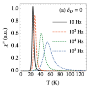
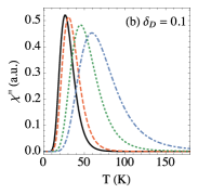
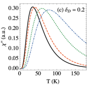
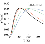
Figure 1: (Color Online) (a) Example curves of $\chi^{\prime\prime}$ vs. $T$ for ideal monodisperse samples computed from Eq. (5) with $\theta=400$ K, $\tau_{0}=10^{-9}$ s and different values of $f$. (b)-(d) Same, but for polidisperse samples, computed from the numerical solution of the integral in Eq. (14), with $\theta_{0}=400$ K and three different values of $\delta_{D}$.

II.2 Magnetic moment of samples with a size distribution

The case of ideal monodisperse samples, where all particles have the exact same volume, is highly improbable in practice. For example, in Ref. Park et al., 2005 a minimum standard deviation of 3% in the diameter was obtained, even though the synthetic method used is known from the literature to produce highly monodisperse MNPs. It is therefore essential to include in any analysis the effects of a size distribution.

If we randomly draw a particle from a sample and measure its diameter $D$, the result will be a random quantity described by a probability distribution $P(D)$. This distribution may be experimentally accessed from TEM measurements by directly counting the number of particles with a given diameter (cf. Figs. 4 and 9 below).

It is also customary to model $P(D)$ by a lognormal distribution

$$P(D)=\frac{1}{\sqrt{2\pi}\delta_{D}D}e^{-\frac{\ln^{2}(D/D_{0})}{2\delta_{D}^{2}}}$$ (8)

with parameters $D_{0}$ and $\delta_{D}$. The parameter $D_{0}$ in Eq. (8) is the median of $P(D)$ and not the average diameter, which reads $D_{0}e^{\delta_{D}^{2}/2}$. Moreover, $\delta_{D}$ is a dimensionless parameter related to the standard deviation (SD) by $\text{SD}=D_{0}e^{\delta_{D}^{2}/2}\sqrt{e^{\delta_{D}^{2}}-1}$. Defining the root-mean-square deviation as the ratio between the standard deviation and the mean diameter, we therefore get

$$\text{r.m.s.}=\sqrt{e^{\delta_{D}^{2}}-1}\simeq\delta_{D}$$ (9)

Hence, $\delta_{D}$ is a measure of the root-mean-square deviation. Samples with $\delta_{D}\lesssim 0.1$ (10%) are usually considered monodisperse in the MNP synthesis literature.

From the distribution of diameters $P(D)$, we may also look at the distribution of volumes $P(V)$. For this purpose, the lognormal distribution turns out to be quite useful since it satisfies the following very unique property: If $D$ is lognormal, then so will $aD^{k}$, with parameters $aD_{0}^{k}$ and $|k|\delta_{D}$. This means that the distribution of volumes $P(V)$ will also be given by a lognormal distribution, which for spherical particles will have parameters $V_{0}=\frac{\pi}{6}D_{0}^{3}$ and $\delta_{V}=3\delta_{D}$ (for non-spherical particles only $V_{0}$ must to be modified). That is, the dispersion parameter of the volume distribution is three times larger than the dispersion parameter of the diameter distribution. Note that this property is not satisfied by other distributions, such as the Gaussian or the Gamma distributions.

Assuming that the anisotropy constant $K$ is the same for all particles, the energy barrier $\theta=KV/k_{B}$ will, for the same reason, also be given by a lognormal distribution

$$P(\theta)=\frac{1}{\sqrt{2\pi}\theta\delta_{\theta}}e^{-\frac{\ln^{2}(\theta/\theta_{0})}{2\delta_{\theta}^{2}}}$$ (10)

with parameters

$$\theta_{0}=\frac{KV_{0}}{k_{B}},\qquad\delta_{\theta}=\delta_{V}=3\delta_{D}$$ (11)

The physical meaning of $P(\theta)$ is that, if you randomly draw a particle from your sample, the probability that it will have an energy barrier between $\theta$ and $\theta+\,\mathrm{d}\theta$ is $P(\theta)\,\mathrm{d}\theta$. All our calculations will be done using $P(\theta)$. The situation where $K$ is not constant will be discussed in Sec. II.6.

In order to model the magnetic properties of samples with a size distribution, we must average results such as Eq. (5), over $P(V)$ or $P(\theta)$. However, this procedure involves a subtle point which has caused considerable confusion in the past. It is related to the distinction between the number distribution of volumes, which is the quantity $P(V)$ obtained from TEM, and another distribution called the volume distribution of volumes. Although subtle, this point determines the form of the static susceptibility $\chi_{0}$ in Eq. (6). And, if one wishes, to compare AC susceptibility experiments with TEM data, it is essential that the correct form of $\chi_{0}$ be used. For a thorough discussion clarifying this point, see Ref. El-Hilo, 2012; *El-Hilo2012. We present here a complementary discussion, based on physical arguments.

The main idea is that in an actual experiment, the signal picked up by the magnetometer is always proportional to the magnetic moment of the particles, never the magnetization. Thus, even though it is customary to work with magnetization when developing theoretical models, the correct quantity to be averaged when considering a size distribution is always the magnetic moment.

Consider any type of experiment, static or dynamic, and let $\mu(V)$ be the magnetic moment of a particle whose volume is $V$ (by $\mu$ we mean the component of the magnetic moment vector being measured by the pick-up coil). Also, suppose that in our sample there are $N_{1}$ particles with volume $V_{1}$, $N_{2}$ particles with volume $V_{2}$, etc. Then the total signal measured by the magnetometer will be

$$\mu_{\text{tot}}=\sum\limits_{i}\mu(V_{i})N_{i}$$ (12)

We may also define

$$p_{i}=\frac{N_{i}}{N}$$

where $N=\sum_{i}N_{i}$ is the total number of particles in the sample. The $p_{i}$ represent the probabilities that a particle randomly drawn from the sample will have a volume $V_{i}$. Thus, they correspond exactly to the quantities measured from TEM. In terms of them, Eq. (12) becomes

$$\mu_{\text{tot}}=N\sum\limits_{i}\mu(V_{i})p_{i}$$

For the purpose of clarity, we have assumed that the distribution of volumes is discrete. In order to turn it into a continuous representation we simply replace the sum by an integral; viz.,

$$\mu_{\text{tot}}=N\int\mu(V)P(V)\,\mathrm{d}V$$ (13)

In conclusion, in order to average a certain property over $P(V)$ or $P(\theta)$, as obtained from TEM, it is always necessary to average the magnetic moment, and not the magnetization.

II.3 AC susceptibility for samples with a size distribution

We are now ready to average Eq. (5) over the size distribution, using Eq. (13). It is more convenient, however, to average over $P(\theta)$ in Eq. (10). Using the definitions $\theta=KV/k_{B}$ and $\theta_{0}=KV_{0}/k_{B}$ to write $V$ in terms of $\theta$ we find that

$$\chi^{\prime\prime}=N\frac{(M_{s}V_{0})^{2}}{3k_{B}T}\int\limits_{0}^{\infty}\frac{\theta^{2}}{\theta_{0}^{2}}\frac{\omega\tau(\theta/T)}{1+[\omega\tau(\theta/T)]^{2}}P(\theta)\,\mathrm{d}\theta$$ (14)

This result is plotted in Figs. 1(b)-(d) for several values of $\delta_{D}$ by numerically solving the integral. In these figures it is possible to see the gradual effect which an increasing size dispersion has on the general shape of the curves.

Eq. (14) is exact, but not very convenient to work with. An approximate formula may be obtained by noting that the function $\frac{\omega\tau}{1+(\omega\tau)^{2}}$ will be sharply peaked around

$$\sigma^{*}=-\ln(2\pi f\tau_{0})$$ (15)

We may therefore approximate $\frac{\omega\tau}{1+(\omega\tau)^{2}}\simeq\frac{\pi}{2}\delta(\sigma-\sigma^{*})$, which leads to

$$\chi^{\prime\prime}\simeq N\frac{\pi(M_{s}V_{0})^{2}}{6k_{B}}\frac{(\sigma^{*}T)^{2}}{\theta_{0}^{2}}P(\sigma^{*}T)$$ (16)

Note that for frequencies of usual interest in AC susceptibility we have $\sigma^{*}>2$, which is the requirement for the validity of Eq. (1).Coffey and Kalmykov (2012)^,64

Eq. (16) is valid for any distribution $P(\theta)$. Specializing to the case of the lognormal distribution, Eq. (10), and defining

$$\theta^{*}=\sigma^{*}T=-T\ln(2\pi f\tau_{0})$$ (17)

we finally arrive atJonsson et al. (1997)

$$\chi^{\prime\prime}=c\frac{\theta^{*}}{\theta_{0}^{2}}\exp{\Bigg{\{}-\frac{\ln^{2}(\theta^{*}/\theta_{0})}{2\delta_{\theta}^{2}}\Bigg{\}}}$$ (18)

where $c=\sqrt{\frac{\pi}{2}}N(M_{s}V_{0})^{2}/(6k_{B}\delta_{\theta})$ is a positive constant. The reason why $\theta_{0}^{2}$ was not included in $c$ is because it is the only term which depends on $K$ and below, in Sec. II.4, we will consider samples which have a distribution of $K$ values. In Figs. 2 we compare Eq. (14) with Eq. (18). It is found that the agreement is overall very good, even for samples with a low dispersion. Slight discrepancies are only observed for monodisperse samples ($\delta_{D}=0.1$) at high frequencies ($f=10$ kHz).

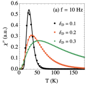
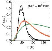
Figure 2: (Color Online) Comparison between the integral formula (14) and the approximate formula (16) for different values of $\delta_{D}$ and different frequencies. The other parameters are the same as in Fig. 1.

Differentiating Eq. (18) with respect to $\theta^{*}=\sigma^{*}T$ we find that the maximum of $\chi^{\prime\prime}$ occurs at $\theta_{0}e^{\delta_{\theta}^{2}}$. This implies the relation

$$-\ln(2\pi f)=\ln(\tau_{0})+\frac{\theta_{0}e^{\delta_{\theta}^{2}}}{T_{\text{max}}}$$ (19)

which shows that even for polidisperse samples an Arrhenius plot will still give a straight line. However, the slope of the line is given by $\theta_{0}e^{\delta_{\theta}^{2}}$. For typical samples we have $\delta_{D}\sim 0.25$, which leads to $\delta_{\theta}=3\delta_{D}\sim 0.75$ and thence $e^{\delta_{\theta}^{2}}\sim 1.75$. This shows that the Arrhenius plot overestimates the anisotropy constant $K$ by a factor which can be almost of the order of 2 in certain cases.

We finish this section by noting that, in general, $\chi^{\prime\prime}$ is a function of both $f$ and $T$. However, under the approximations that led to Eqs. (16) or (18), it turns out that $\chi^{\prime\prime}$ will only depend on the particular combination $\theta^{*}=\sigma^{*}T=-T\ln(2\pi f\tau_{0})$. This means that if we plot each $\chi^{\prime\prime}$ curve as a function of $\theta^{*}$ instead of $T$, the data for different frequencies should all collapse into a single curve, provided $\tau_{0}$ is correctly chosen. Hence, this method may be used to determine $\tau_{0}$ and, since it uses the entire $\chi^{\prime\prime}(f,T)$ data set, it turns out to be much more precise than the Arrhenius plot. Examples of this are given below for our data in Figs. 5 and 10 or, e.g., in Refs. Masunaga et al., 2009; *Masunaga2011b and Jonsson et al., 1997. The collapsed data will be described by Eq. (18), which depends only on $\delta_{\theta}$, $\theta_{0}$ and $c$. But $\delta_{\theta}=3\delta_{D}$ is already known from TEM, so that the only two fit parameters are $c$ and $\theta_{0}$. From Eq. (11), $\theta_{0}=KV_{0}/k_{B}$ and $V_{0}$ is also known from TEM, so that we may extract the anisotropy constant $K$.

II.4 Variation of $\chi_{\text{max}}^{\prime\prime}$ with frequency

The usual Arrhenius analysis of AC susceptibility data focuses on the temperature $T_{\text{max}}$ where $\chi^{\prime\prime}$ is a maximum. We now argue that valuable information concerning the dipolar interaction is contained in the height of these peaks. Let us denote the maximum of each $\chi^{\prime\prime}$ vs. $T$ curve as $\chi_{\text{max}}^{\prime\prime}$. In Fig. 1 we see two possible behaviors: For monodisperse samples, $\chi_{\text{max}}^{\prime\prime}$ decreases with $f$, whereas for polidisperse samples, $\chi_{\text{max}}^{\prime\prime}$ tends to become roughly constant, independent of $f$. These are the only two possibilities predicted by models of non-interacting particles, including the full Fokker-Planck description of the stochastic Landau-Lifshitz-Gilbert equation.Brown (1963); *Brown1979a; Coffey et al. (2004); Poperechny et al. (2010); Landi (2012a); *Landi2012b; *Landi2012e

However, in real samples it is also customary to find situations where $\chi_{\text{max}}^{\prime\prime}$ increases with $f$. We argue that this is a signature of a strong dipolar interaction. It therefore serves as a simple test to estimate the extent of this interaction in a given sample. If $\chi_{\text{max}}^{\prime\prime}$ increases with $f$, the dipolar contribution certainly has a significant effect. This requires no sophisticated analyses, just a simple glimpse at the $\chi^{\prime\prime}$ curves for different frequencies (this effect was briefly commented in Ref. Hansen et al., 2002). Please note that this rule is only valid for the imaginary part $\chi^{\prime\prime}$. It does not hold for the real part $\chi^{\prime}$.

Our claim is corroborated by extensive experimental evidence in the literature. The most clear examples are Refs. Masunaga et al., 2009; *Masunaga2011b; Jonsson et al., 1998a; Djurberg et al., 1997; Jönsson et al., 2000; Hansen et al., 2002, which study samples with different concentrations. In all cases the results are unambiguous: for diluted samples $\chi_{\text{max}}^{\prime\prime}$ is either constant or diminishes with $f$, whereas for concentrated samples $\chi_{\text{max}}^{\prime\prime}$ increases with $f$. Additional examples may also be found in Refs. Aslibeiki et al., 2010; Bittova et al., 2012; Goya et al., 2003; Jonsson et al., 1998b; Kleemann et al., 2001; Monson et al., 2013; Parker et al., 2008; Roca et al., 2012; Winkler et al., 2008; Zhang et al., 1996 and in Figs. 5 and 10.

The dipolar interaction creates a tendency for $\chi_{\text{max}}^{\prime\prime}$ to increase with $f$. But, if the sample is monodisperse, $\chi_{\text{max}}^{\prime\prime}$ naturally decreases with $f$. Hence, in these cases there is a competition between the two effects and care must be taken in analyzing the results. This is well illustrated in Figs. 7 and 8 of Ref. Berkov and Gorn, 2001, where the authors simulate the AC susceptibility response of interacting ideally monodisperse particles using the Stochastic Landau-Lifshitz equation. They find that, depending on the several parameters of the sample, $\chi_{\text{max}}^{\prime\prime}$ may either decrease or increase with $f$. In Table 1 we summarize the different possible behaviors of $\chi_{\text{max}}^{\prime\prime}$ with $f$.

Table 1: How the maximum of the imaginary part, $\chi_{\text{max}}^{\prime\prime}$, behaves with the frequency $f$.

	Monodisperse	Polidisperse
Non-interacting	Decreases	Constant
Interacting	Inconclusive	Increases

II.5 Formulas for the susceptibility including the dipolar interaction

We will now consider how Eq. (18) may be modified to include models of the dipolar interaction. We shall focus on three distinct models: the Vogel-Fulcher approximationShtrikman and Wohlfarth (1981), a mean-field variant of this law developed recently in Ref. Landi, 2013; *Landi2014 and the Dormann-Bessais-Fiorani (DBF) model.Dormann et al. (1999) This will provide us with a tool to include the dipolar effect in the susceptibility analysis and will also serve to further corroborate our claim on the dependence of $\chi_{\text{max}}^{\prime\prime}$ with $f$. It is important to clarify upfront, however, that due to the enormous complexity of the interaction, any model will always involve an enormous number of approximations and, inevitably, will only be able to capture a fraction of the real phenomenon.

The most popular model for the dipolar interaction is the Vogel-Fulcher law,Shtrikman and Wohlfarth (1981) whereby the energy barrier parameter $\sigma$ is modified to account for the dipolar interaction according to

$$\sigma_{\text{VF}}=\frac{\theta}{T-T_{\text{VF}}}$$ (20)

where $T_{\text{VF}}$ provides a measure of the strength of the dipolar interaction. To study how this modification affects the AC curves we insert Eq. (20) in Eq. (14) and compute the integral numerically. The results are shown in Fig. 3 for parameters similar to those in Fig. (1). It can be seen that the larger is $T_{\text{VF}}$, the stronger is the increase of $\chi_{\text{max}}^{\prime\prime}$ with $f$. The competition that occurs for monodisperse samples is also evident, particularly when Fig. 3(a) is compared with Fig. 1(b).

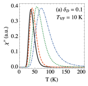
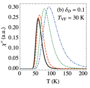
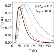
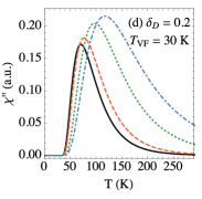
Figure 3: Effect of the Vogel-Fulcher modification, Eq. (20), in the AC susceptibility curves. The simulation parameters are shown in the caption of each figure. The other parameters are the same as in Fig. 1.

In Fig. 3 it can also be seen that for $T<T_{\text{VF}}$ the susceptibility is identically zero. However, such a zero susceptibility is never observed in real samples, showing an apparent inconsistency of the Vogel-Fulcher law. Namely that the value of $T_{\text{VF}}$, usually obtained from an Arrhenius plot, is not compatible with the original model from which it was derived. This, of course, is just a reflection of the fact that Eq. (20) is an approximate model to describe an extremely complex effect. It therefore can only contain a certain share of the real contribution from the dipolar interaction.

Recently, one of the authors of this paper has worked out a mean-field model to describe the dipolar interaction.Landi (2013); *Landi2014 The main result of this model is that, instead of Eq. (20), we should have for sufficiently weak dipolar coupling,

$$\sigma_{\text{MF}}=\frac{\theta}{T}+\gamma\left(\frac{\theta}{T}\right)^{2}$$ (21)

whereLandi (2013); *Landi2014

$$\gamma=\frac{N}{10}\left(\frac{\mu_{0}}{4\pi}\right)^{2}\left(\frac{\langle\mu^{2}\rangle}{KV_{0}}\right)^{2}\left\langle\frac{1}{R^{6}}\right\rangle\sim T_{\text{VF}}/\theta_{0}$$ (22)

is a dimensionless parameter representing the strength of the dipolar interaction. In this formula $N$ is the number of particles in the sample, $\mu_{0}$ is the vacuum permeability$,\langle\mu^{2}\rangle$ is the average magnetic moment squared in the sample and $R$ is the random variable representing the distance between particles in the sample. Eq. (21) gives results which are qualitatively similar to those of the Vogel-Fulcher model. However, it has the advantage that it does not predict a zero susceptibility below a certain temperature.

The mean-field approximation (21) is also more convenient than the Vogel-Fulcher model if one wishes to simplify the integral formula (14) as we did when deriving Eq. (18). We shall therefore now retrace these steps, using instead the modified $\sigma_{\text{MF}}$ of Eq. (21). First, the maximum of $\omega\tau/(1+(\omega\tau)^{2})$ will now occur at

$$\sigma_{\text{MF}}^{*}=\frac{1}{2\gamma}\Bigg{[}\sqrt{1-4\gamma\ln(2\pi f\tau_{0})}-1\Bigg{]}$$ (23)

Moreover, taking into account the relevant experimental ranges for the frequencies $f$, we may approximate

$$\frac{\omega\tau}{1+(\omega\tau)^{2}}\simeq\frac{\pi}{2}\frac{1}{\sqrt{1-4\gamma\ln(2\pi f\tau_{0})}}\delta(\sigma-\sigma^{*})$$

Let us define

$$\psi(f,\gamma)=\frac{1}{\sqrt{1-4\gamma\ln(2\pi f\tau_{0})}}$$ (24)

Then Eq. (14) may be approximated to

$$\chi^{\prime\prime}\simeq N\frac{\pi(M_{s}V_{0})^{2}}{6k_{B}}\psi(f,\gamma)\frac{(\sigma_{\text{MF}}^{*}T)^{2}}{\theta_{0}^{2}}P(\sigma_{\text{MF}}^{*}T)$$ (25)

Notice how the dependence of $\chi_{\text{max}}^{\prime\prime}$ with $f$ now appears explicitly through the function $\psi(f,\gamma)$. The mean-field model therefore predicts that $\chi_{\text{max}}^{\prime\prime}$ should increase roughly logarithmically (for small $\gamma$) with $f$. A numerical analysis shows a similar dependence for the Vogel-Fulcher approximation.

We may now finally write the modified version of Eq. (18), which includes the explicit assumption of a lognormal distribution:

$$\chi^{\prime\prime}=c\;\psi(f,\gamma)\frac{\theta^{*}}{\theta_{0}^{2}}\exp{\Bigg{\{}-\frac{\ln^{2}(\theta^{*}/\theta_{0})}{2\delta_{\theta}^{2}}\Bigg{\}}}$$ (26)

where, now

$$\theta^{*}=\sigma_{\text{MF}}^{*}T=\frac{T}{2\gamma}\Bigg{[}\sqrt{1-4\gamma\ln(2\pi f\tau_{0})}-1\Bigg{]}$$ (27)

According to these results, we see that in the weakly interacting case [which is where the mean-field approximation (21) applies] one should be able to perform a data collapse by plotting $\chi^{\prime\prime}/\psi$ vs. $\theta^{*}$.

Both previous models hold for weakly interacting systems. In the case of strong interactions, the DBF modelDormann et al. (1999) predicts instead that the relaxation time of the system should be modified according to

$$\tau=\tau_{0}e^{-n_{1}}\exp\bigg{\{}\sigma\left(1+\frac{n_{1}a_{1}M_{s}^{2}}{K}\right)\bigg{\}}$$ (28)

where $n_{1}$ is the number of nearest neighbors and $a_{1}$ is the volume concentration of particles in the sample. This model therefore predicts two results. First, that $\tau_{0}$ should be effectively reduced by a factor $e^{-n_{1}}$. This explains the unphysically low $\tau_{0}$ values which are sometimes obtained using Arrhenius plots. Second, it predicts an increase in the energy barrier $\sigma$ according to

$$\sigma_{\text{DBF}}=\sigma\left(1+\frac{n_{1}a_{1}M_{s}^{2}}{K}\right)$$

Notice that the $\sigma$ (or $V$) dependence is linear in this case and not non-linear as in Eqs. (20) and (21). Consequently, the DBF model would not predict a change in the height of the $\chi^{\prime\prime}$ vs. $T$ curves in the strongly interacting regime.

II.6 Distribution of anisotropy constants

As discussed in Sec. I, in addition to the usual contribution from the dipolar interaction, we must also consider the distribution of anisotropy constants caused by the formation of aggregates. The particles in a sample are either in free suspension in the fluid or reside in clusters of different sizes.Castro et al. (2008) And depending on the size of the cluster a particle resides and in the position of the particle within that cluster, it may experience a different modification to its anisotropy constant $K$.Jacobs and Bean (1955); Branquinho et al. (2013) We therefore see that, in addition to the distribution of volumes in a given sample, we should also expect to have a very complex distribution of $K$ values. This effect is likely much more significant than the intrinsic fluctuations due to the crystallinity, shape and surface roughness that exist in every sample.

To include this effect, we must perform a second average of Eq. (26) over a distribution of $K$. This distribution is certainly continuous, but we have no information about it to be able to propose an analytical formula. Hence, we will for simplicity assume that the distribution of anisotropy constants is discrete. That is, we will assume that in the sample there is a fraction $q_{1}$ of particles which have an anisotropy constant $K_{1}$, a fraction $q_{2}$ with constant $K_{2}$, etc. In order to obtain a tractable equation, we will also assume that $\gamma$ defined in Eq. (22) is the same for all $K$, an approximation which is justified due to the smallness of $\gamma$. We then obtain, instead of Eq. (26),

$$\chi^{\prime\prime}=c\;\psi(f,\gamma)\sum\limits_{i=1}^{n_{K}}q_{i}\frac{\theta^{*}}{\theta_{0,i}^{2}}\exp{\Bigg{\{}-\frac{\ln^{2}(\theta^{*}/\theta_{0,i})}{2\delta_{\theta}^{2}}\Bigg{\}}}$$ (29)

where $n_{K}$ is the total number of distinct $K$ values we wish to consider and

$$\theta_{0,i}=\frac{K_{i}V_{0}}{k_{B}}$$ (30)

with $V_{0}$ being known from TEM. Eq. (29) can be fitted to the collapsed data, with parameters $c$, $q_{i}$ and $\theta_{0,i}$ (the value of $\delta_{\theta}$ is fixed from TEM).

Each $K_{i}$ symbolically represents an environment in which the particle may reside and the $q_{i}$ represents the fraction of the total population of particles in that environment. By “environment” we mean, for instance, a cluster of a given size or the position of the particle within a cluster. Due to the enormous complexity of the spatial arrangement of the particles in a sample, it is not possible to make a quantitative definition of the type and number of environments. Instead, the purpose of this procedure, is to quantify the importance of the dipolar interaction in the sample and the complexity of the particle arrangements. If a given sample requires a large number of $K_{i}$ values to be adequately described by Eq. (29), then the dipolar interaction is likely producing a complex modification in the energy landscape of the particles. Moreover, by analyzing the different $K_{i}$ values obtained for each sample and comparing them with the expected $K_{i}$ values of a non-interacting ensemble, we may infer the types of modifications brought about by particle aggregation.

As a final technical comment, we should mention that in principle $\tau_{0}$ also depends on $K$, so we should use different $\tau_{0}$ values for each term in the sum (29). However, the influence of $\tau_{0}$ in the susceptibility is logarithmic and we have found that adding this additional complication produces no improvements whatsoever in the numerical analyzes. We have therefore opted to assume a fixed $\tau_{0}$ for all populations.

III Experiments

We now apply Eq. (29) to two distinct samples. In Sec. III.1 we study a commercial ferrofluid containing spherical magnetite nanoparticles of roughly 6.4 nm in diameter and in Sec. III.2 we study a sample of cubic magnetite nanoparticles with about 13 nm loaded on the surface of PLGA nanospheres. Both samples are studied under different dilutions. All non-linear fits to be presented below were performed using a combination of the Nelder-Mead and Differential Evolution methods. Each fit was repeated several times with different initial random seeds and the result which led to the smallest global merit function was used.

III.1 Spherical magnetite nanoparticles

We begin with the commercial ferrofluid EMG909 from Ferrotec Co, consisting of roughly spherical magnetite particles dispersed in oil. A typical TEM micrograph is shown in Fig. 4 together with the size distribution histogram and lognormal fit. The best fit parameters were $D_{0}=6.4$ nm and $\delta_{D}=0.26$. Thus, the mean diameter is 6.6 nm and the dispersion of the energy barrier distribution is $\delta_{\theta}=3\delta_{D}=0.78$.

We have performed AC susceptibility measurements for three dilutions with volume concentrations of magnetic material of 0.0054%, 0.54% and 3.6%. We shall henceforth refer to them as samples A, B and C respectively. The measurements were performed using a Tesla superconducting quantum interference device (SQUID) from Quantum Design under a field amplitude of 2.0 Oe (0.16 kA/m). The raw data for $\chi^{\prime\prime}$ is shown in Fig. 5(a)-(c). As can be seen, the maximum height $\chi_{\text{max}}^{\prime\prime}$ increases substantially with $f$, indicating the strong presence of the dipolar interaction, even in the most diluted sample. This is likely due to the formation of aggregates since the contribution from isolated monomers randomly distributed in the liquid would be very low. The degree of aggregation may be strongly influenced by several experimental parameters during the synthesis and stable suspension of the nanoparticles. For instance, an inadequate surface coating may decrease the steric and ionic repulsions, leading to a higher degree of aggregation. Another possibility is the aging of the MNPs, which may lead to a desorption mechanism of the coating molecules.Bakuzis et al. (2013); *Castro2008; *Eloi2010 The temperature where $\chi^{\prime\prime}$ is maximum also shifts to higher values as the sample concentration is increased.

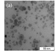
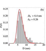
Figure 4: (a) TEM micrograph of the commercial ferrofluid EMG909 from Ferrotec Co. (b) Corresponding size distribution and lognormal fit. Best fit parameters are shown in the figure.

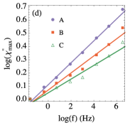
Figure 5: Raw AC susceptibility data for several frequencies for samples (a) A, (b) B and (c) C. The volume concentrations of magnetic material were 0.0054%, 0.54% and 3.6% respectively. Image (d) shows a log-log plot of the maximum of each $\chi^{\prime\prime}$ curve as a function of the frequency $f$ for the three samples. Each curve was normalized for visual purposes in order to start at the same point. The solid lines correspond to linear fits with exponents 0.083, 0.064 and 0.052 for samples A, B and C respectively.

In Fig. 5(d) we present a log-log plot of the maximum height, $\chi_{\text{max}}^{\prime\prime}$, of each $\chi^{\prime\prime}$ vs. $T$ curve as a function of the frequency $f$. The linearity of the data in a log-log plot shows that $\chi_{\text{max}}^{\prime\prime}$ depends on $f$ according a power law behavior

$$\chi_{\text{max}}^{\prime\prime}\sim f^{\alpha}$$ (31)

for some exponent $\alpha$. The values of $\alpha$ obtained from a linear fit were 0.083, 0.064 and 0.052 for samples A, B and C respectively. This behavior is quite different from that predicted by the mean-field model [Eq. (24)], whereby $\chi_{\text{max}}^{\prime\prime}$ should depend only logarithmically on $f$. This discrepancy, as already pointed out in Sec. II.5, is actually expected given that the mean-field model only holds for weakly-interacting particles.

We now attempt to perform a data collapse of the $\chi^{\prime\prime}$ data. To do so, we first normalize all curves to have the same height since this aspect has already been analyzed in Eq. (31). Next we must consider the choice of $\theta^{*}$ to be used. For non-interacting samples, we should use Eq. (17) and attempt to obtain a single $\tau_{0}$ value which adequately fits all three samples. Conversely, for interacting samples we could attempt to use Eq. (27), even though we already know from the height analysis that the latter should not be very precise. In this case we should try to obtain a $\tau_{0}$ value which is the same for all three samples, but different $\gamma$ values for each sample.

The results for both cases are visually identical and for simplicity we only present one, shown in Fig. 6. If Eq. (17) is used, we obtain $\tau_{0}=2\times 10^{-10}$ s, but if Eq. (27) is used we obtain $\tau_{0}=2\times 10^{-9}$ s and $\gamma=0.01$, 0.01 and 0.0115 for samples A, B and C respectively. We therefore see that by neglecting the dipolar interaction, we underestimate $\tau_{0}$ by one order of magnitude. This, as mentioned above, is a frequent problem in the analysis of interacting particles. According to Eq. (28) the presence of the dipolar interaction should modify $\tau_{0}$ by a factor $e^{-n_{1}}$, where $n_{1}$ is the average number of nearest neighbors. Thus, we may estimate this value by analyzing the ratio between our two estimates of $\tau_{0}$, the one with the dipolar interaction and the one without it. As a result we get $n_{1}\simeq 2.3$.

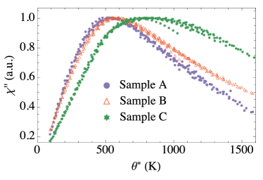
Figure 6: Data collapse for samples A, B and C, obtained by plotting $\chi^{\prime\prime}$ as a function of $\theta^{*}$, defined either in Eq. (17) or Eq. (27). The results are visually identical in both cases. If Eq. (17) is used, we obtain $\tau_{0}=2\times 10^{-10}$ s, but if Eq. (27) is used we obtain $\tau_{0}=2\times 10^{-9}$ s and $\gamma=0.01$, 0.01 and 0.0115 for samples A, B and C respectively.

Once we have obtained a collapsed set of data, the long-range manifestation of the dipolar interaction has been completely accounted for and we may proceed to use Eq. (29) in order to study the aggregation of particles within the sample. Thus, we shall now fit the collapsed data sets using Eq. (29). From TEM we already know that $\delta_{\theta}=3\delta_{D}=0.78$ so the only free parameters are $\theta_{0,i}$, $q_{i}$ and $c$. The results for $n_{K}=1$ are shown in the left panel of Fig. 7 and the best fit values of $\theta_{0}$ are presented in each image. A clear disagreement between the fitted curve and the experimental data can be observed. The situation is particularly worse at low temperatures, where the signal from smaller particles is expected to be stronger. Note also that this discrepancy is not related to the fact that we fixed $\delta_{\theta}$; leaving it as a free parameter would not improve the results.

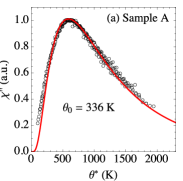
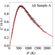
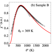
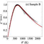
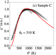
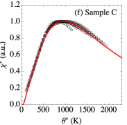
Figure 7: Fit of Eq. (29) to the AC susceptibility data of samples A, B and C. Left panel: $n_{K}=1$. Right panel: $n_{K}=2$. Best fit results for the left panel are shown in each image and for the right panel in Table 2.

Table 2: Best fit values of Eq. (29) for samples A, B and C when $n_{K}=2$.

Sample A			Sample B			Sample C
$\theta_{0,i}$ (K)	$q_{i}$		$\theta_{0,i}$ (K)	$q_{i}$		$\theta_{0,i}$ (K)	$q_{i}$
67	0.026		89	0.039		137	0.04
387	0.974		438	0.961		625	0.96

Motivated by this, we now attempt to fit Eq. (29) using two $K$ values ($n_{K}=2$). The results are shown in the right panel of Fig. 7 and the best fit parameters are presented in Table 2. As can be seen, in this case the agreement with the experimental data is remarkably good. From Table 2 we see that both $\theta_{0,1}$ and $\theta_{0,2}$ increase with concentration, indicating that the dipolar interaction shifts the energy barrier distribution of the particles to higher values. In Table 2 we also report the fractions $q_{i}$, showing that the majority of the particles have a high anisotropy. Notwithstanding, since Eq. (29) depends on $1/\theta_{0,i}^{2}$, the small fraction $q_{1}$ still gives a significant contribution to the AC susceptibility curve, specially at low temperatures.

For completeness, we present in Fig. 8 an Arrhenius plot [cf. Eq. (19)] for the three samples. The corresponding best-fit parameters are shown in the figure. As can be seen, the Arrhenius plot predicts distinct values of $\tau_{0}$ for each dilution, which fluctuate substantially. This is related to the strong sensitivity of the Arrhenius plot to experimental uncertainties. Moreover, the values of $\theta_{0}$ are somewhat similar to those obtained using $n_{K}=1$ in the left part of Fig. 7.

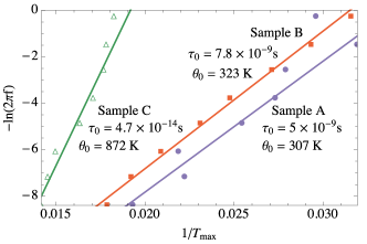
Figure 8: Arrhenius plots [Eq. (19)] for samples A, B and C. The best fit parameters are shown in the figure. In the computation of $\theta_{0}$ it is necessary to use $\delta_{\theta}=3\delta_{D}=0.78$.

We used a bimodal distribution and obtained the constants $\theta_{0,1}$ and $\theta_{0,2}$ reported in Table 2, together with the populations $q_{1}$ and $q_{2}$. The values of $K_{1}$ and $K_{2}$ are then obtained from the relations $\theta_{0,i}=K_{i}V_{0}/k_{B}$. For this sample $k_{B}/V_{0}\simeq 1000$ erg/(K cm³) $=0.1$ kJ/(K m³). Hence, using the data from Table 2 we conclude that the particles in smaller aggregates have anisotropy constants between 6 and 14 kJ/m³. Conversely, the particles residing in large aggregates have anisotropy constants between 38 and 63 kJ/m³.

We therefore observe a roughly 5-fold increase in the effective anisotropy constants between the two populations. Such a large difference requires a more careful analysis. In Ref. Branquinho et al., 2013; Bakuzis et al., 2013; *Castro2008; *Eloi2010 one of the authors studied a microscopic model of particle aggregation for linear chains, which is the structure expected for colloids within this concentration range. It was found that the typical changes in effective anisotropy between chains of different sizes was usually around 2-fold, reaching at most up to 3-fold for certain nanoparticle arrangements. The 5-fold change observed in this sample therefore suggests that the size distribution of the particles in different aggregates may not be the same. That is, larger clusters have a tendency to contain larger particles and vice-versa.

III.2 Cubic magnetite nanoparticles

Next we consider the case of PLGA nanospheres loaded with cubic magnetite nanoparticles. The confinement of the nanoparticles in the PLGA nanospheres allows maintaining a fixed arrangement of the nanoparticles and prevent uncontrolled aggregation upon increasing concentration. The nanocubes are placed on the surface of the nanospheres, forming quasi 2-dimensional aggregates. The details of the synthesis and additional characterization of this sample can be found in Ref. Andreu et al., 2015b.

All results developed in Sec. II also hold for cubic particles, provided we now use $V_{0}=D_{0}^{3}/2^{3/2}$ where $D_{0}$ is the face diagonal of the cubes. Fig. 9(a) and (b) show a typical TEM image of the particles together with the size distribution histogram and the lognormal fit. The best fit parameters were $D_{0}=13.1$ nm and $\delta_{D}=0.11$, showing that the size distribution is very narrow. Indeed, referring to Eq. (9), we see that these nano-cubes may be considered as monodisperse.Andreu et al. (2015b) In Fig. 9(c) we also show an example of the PLGA nanospheres loaded with MNPs.

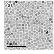
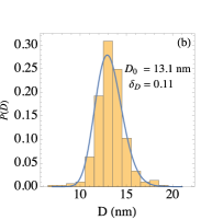
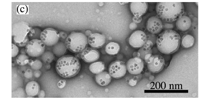
Figure 9: (a) TEM micrograph of the cubic magnetite nanoparticles. (b) Distribution of face diagonals $D$ and corresponding lognormal fit. The best fit parameters are shown in the figure. (c) Example of the nanoparticles loaded into PLGA nanospheres.

We have performed AC susceptibility measurements on these nanoparticles in two configurations; namely with the PLGA spheres dispersed in water and with them lyophilized to form a powder. We shall refer to them as samples L and S respectively. In these samples, the nanocube arrangements are preserved, but the inter-sphere distance is changed (shorter in S). The volume concentration of magnetic material is 0.001% and 0.783% respectively for samples L and S. In Fig. 10 we present the raw susceptibility data for both samples and several frequencies, acquired with an MPMS-XL SQUID from Quantum Design under a field amplitude of 2.74 Oe (0.22 kA/m). As can be seen, in both cases there is a sensitive dependence of $\chi_{\text{max}}^{\prime\prime}$ with the height, indicating the presence of a sizable dipolar contribution. This is due to the compact arrangement of the particles inside the nanospheres.

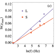
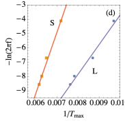
Figure 10: (a),(b) Raw AC susceptibility data for samples L (dispersed in water) and S (lyophilized) of cubic magnetic particles. The volume concentration of magnetic material was 0.001% and 0.783% respectively for samples L and S. (c) Maximum height $\chi_{\text{max}}^{\prime\prime}$ as a function of $f$ (normalized by the first frequency point). (d) Arrhenius plot with best fit parameters $\tau_{0}=2.45\times 10^{-11}$ s and $\theta_{0}=2073$ K for sample L and $\tau_{0}=8.59\times 10^{-16}$ s and $\theta_{0}=4256$ K for sample S.

We begin, as before, by analyzing the dependence of $\chi_{\text{max}}^{\prime\prime}$ with $f$. The results are shown in Fig. 10(c) where we again observe an approximate power law behavior [cf. Eq. (31)], with exponents $\alpha=$ 0.019 and 0.013 for samples L and S respectively. We also perform an Arrhenius plot shown in Fig. 10(d). The linear fit yields $\tau_{0}=2.45\times 10^{-11}$ s and $\theta_{0}=2073$ K for sample L and $\tau_{0}=8.59\times 10^{-16}$ s and $\theta_{0}=4256$ K for sample S. We therefore see a clear discrepancy in the $\tau_{0}$ values, which should be the same since both samples are composed by the exact same particles. Moreover, we see that for sample S the value of $\tau_{0}$ is clearly unphysical. This is again a manifestation of the influence of the dipolar interaction in estimating $\tau_{0}$.

This problem with $\tau_{0}$ can be resolved by performing the data collapse of the data using Eqs. (17) and (27). The results are again visually identical and are shown in Fig. 11. If Eq. (17) is used, we obtain $\tau_{0}=5\times 10^{-16}$ s, but if Eq. (27) is used we obtain $\tau_{0}=4\times 10^{-10}$ s and $\gamma=0.6$ and 0.9 for samples L and S respectively. We see that neglecting the dipolar interaction yields an unphysical value of $\tau_{0}$, similar to that of the Arrhenius plot. But including the mean-field approximation corrects this anomalous behavior. The number of nearest neighbors may again be estimated by comparing the $\tau_{0}$ values obtained by the two different models and using Eq. (28). We find $n_{1}\simeq 13.8$, which correlates well with what is expected from the encapsulation of the MNPs in nano-spheres [cf. Fig. 9(c)].

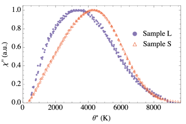
Figure 11: Data collapse for samples L and S, obtained by plotting $\chi^{\prime\prime}$ as a function of $\theta^{*}$, defined either in Eq. (17) or Eq. (27). The results are visually identical in both cases. If Eq. (17) is used, we obtain $\tau_{0}=5\times 10^{-16}$ s, but if Eq. (27) is used we obtain $\tau_{0}=4\times 10^{-10}$ s and $\gamma=0.6$ and 0.9 for samples L and S respectively.

We now fit Eq. (29) to the collapsed data in Fig. 10(c) using $\delta_{\theta}=3\delta_{D}=0.33$, as obtained from TEM. The fits were performed using $n_{K}=1$, 2 and 3 and the results are shown in Fig. 12, for sample L in the left panel and sample S in the right panel. The corresponding best fit parameters are summarized in Table  3. As can be seen, there is a strong disagreement between the best fitted function and the experimental data when $n_{K}=1$ [images (a) and (d)]. The same is true for $n_{K}=2$, despite a visible improvement. It is only for $n_{K}=3$ that the fitted curve begins to resemble the real data. As before, this picture does not change if we allow $\delta_{\theta}$ to be a free parameter. For $n_{K}=3$ the results are better for sample L than sample S, in agreement with our intuition that for sample S the distribution of $K$ values should be much more complex due to the increase of inter-sphere interactions. Increasing $n_{K}$ above 3 does not improve the results in any way.

The results for $n_{K}=3$ shown in Table 3 are quite interesting to analyze. In going from sample L to sample S we see that the energy barriers remain roughly unaltered and only the population of each cluster change. This is in agreement with the fact that both samples have the same nanoparticle arrangement. In summary, from TEM we have found that $D_{0}=13.1$ nm (which refers to the face diagonal) and $\delta_{D}=0.11$. From the data collapse we found $\tau_{0}=5\times 10^{-16}$ s. And, from the fits of the collapsed data, we found that at least three distinct $K$ values are required to correctly describe the data. These values of $K$ may be computed using $\theta_{0,i}$ from Table 3 are roughly 15, 32 and 64 kJ/m³.

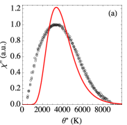
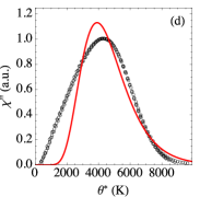
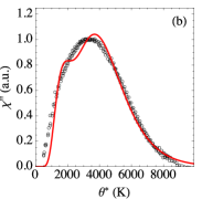
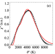
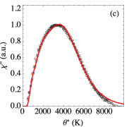
Figure 12: Fit of Eq. (29) to the susceptibility data of samples L (left panel) and S (right panel). (a) and (d): $n_{K}=1$; (b) and (e): $n_{K}=2$; (c) and (f): $n_{K}=3$. The best fit parameters are summarized in Table 3.

Table 3: Best fit values of Eq. (29) for samples L and S, with different values of $n_{K}$. Other important parameters are $D_{0}=13.1$ nm, $\delta_{D}=0.11$ and $\tau_{0}=5\times 10^{-16}$ s.

	Sample L			Sample S
$n_{K}$	$\theta_{0,i}$ (K)	$q_{i}$		$\theta_{0,i}$ (K)	$q_{i}$
1	3000	1		3471	1
2	1539	0.25		1606	0.17
	3444	0.75		3707	0.83
3	916	0.064		818	0.0258
	1833	0.261		1751	0.166
	3590	0.675		3747	0.8082

IV Discussion and conclusions

The purpose of this paper was to show how AC susceptibility, a technique which is nowadays easily accessible in the laboratory, may be used to extract information concerning the importance of the dipolar interaction in the sample. As we have argued, in samples where the particles are left in fluid suspension or packed inside nano-carriers, the dipolar interaction manifests itself in two separate ways. The first is the direct dipolar effect, which can be modeled, for instance, using the Vogel-Fulcher, mean-field or DBF models, as discussed in Sec. II.5. In addition, the dipolar interaction also manifests itself by inducing the formation of clusters of particles within the sample. Once in a cluster, the effective anisotropy of a particle will be strongly modified due to its proximity with the other particles. In this paper we have introduced the idea that this effect can be modeled by including, in addition to the volume distribution usually obtained from TEM, a distribution of anisotropy constants. Even though it is not possible to say much about this distribution in general grounds, we have shown that by proposing a simple discrete probability distribution this approach can be used to probe the complexity of the dipolar interaction in a sample.

In principle, both contributions should be intertwined. However, as we have shown, it is possible to roughly separate the two aspects of the problem by collapsing the data of $\chi^{\prime\prime}$ obtained for different frequencies. The procedure that leads to a collapsed data set involves only the first aspect of the dipolar interaction, whereas the information extracted from the collapsed data involve only the second aspect.

Practically all models and papers discussing the dipolar interaction focus only on the first aspect. It was the purpose of this paper to emphasize the importance of the second aspect as well, specially for samples which are of importance for biological applications.

Both parts of the problem are delicate and must be considered in detail. For the first, as we have shown, none of the three models considered in Sec. II.5 can alone account for all aspects of the experimental data. Notwithstanding, a judicious comparison of the results predicted from each model does allow us to extract physically meaningful information.

For the second part, it is important that we rule out any other possibilities that may explain the discrepancies found when trying to fit just a single $K$ value. First, to explain this using only the size distribution would require a large concentration of particles with very small diameter, but no evidence of this was found in either sample. Secondly, all the approximations that led us to Eq. (18) have been verified, as already demonstrated in Fig. 2. It is also known that Eq. (14) neglects other relaxation times of the particle, such as the transverse relaxation time. But these only manifest themselves at very high frequencies, which is not the case here.Svedlindh et al. (1997); Figueroa et al. (2013) Note also that Brownian relaxation is not allowed since the measurements were performed with the solvents frozen. Finally, this discrepancy also cannot be explained by a Vogel-Fulcher or mean-field theories discussed in Sec. II.4.

It was also the purpose of this paper to call attention to the dependence of $\chi_{\text{max}}^{\prime\prime}$ with $f$. This, as we have shown, provides one with a very simple visual tool to estimate the relevance of the dipolar interaction when analyzing a given sample. A summary of the expected behaviors is shown in Table 1.

In conclusion, we hope to have shown the enormous power of AC susceptibility measurements in extracting information about the dipolar interaction in a sample. First, by a visual analysis $\chi_{\text{max}}^{\prime\prime}$ vs. $f$ one estimates the importance of the dipolar interaction in that sample. Then, using a data collapse one can estimate $\tau_{0}$ and obtain the mean-field interaction constants $\gamma$ defined in Eq. (22) and the mean number of nearest-neighbors $n_{1}$ using Eq. (28). Finally, by fitting the collapsed data using Eq. (29) one is able to probe the complexity of the dipolar landscape and estimate the anisotropy constant distribution in the sample. We hope that the theoretical development described here may be of use to researchers working with magnetic nanoparticles, specially in biological applications such as magnetic hyperthermia. Moreover, we believe that these results illustrate the enormous importance that the dipolar interaction has in most nanoparticle samples.

Appendix A Linear Response Theory

In this appendix we give a general derivation of Eqs. (4) and (5), which is valid also for other materials, such as electric dipoles for instance. Suppose a sample is subject to a time-varying field $H(t)$ pointing in a certain direction and let $\mu(t)$ denote the response of the system in this particular direction. Linear response theory is based on the physically reasonable assumption that if the stimulus $H(t)$ is sufficiently small, the response $\mu(t)$ will be linear in it. However, this does not mean that $\mu(t)$ will depend on the instantaneous value of $H(t)$. It may very well depend on its past values. Thus, we may write in general that

$$\mu(t)=\int\limits_{-\infty}^{t}f(t-s)H(s)\,\mathrm{d}s=\int\limits_{0}^{\infty}f(t^{\prime})H(t-t^{\prime})\,\mathrm{d}t^{\prime}$$ (32)

where in the last equality we simply changed variables to $t^{\prime}=t-s$. The weight function $f(t-s)$ is called the response kernel of the sample and, as far as linear response is concerned, it contains all the relevant information.

We will now analyze a series of experiments. Suppose first that $H(t)$ was turned on at a constant value $H_{0}$ in the infinite past. So the system has had a very long time to stabilize. Inserting $H(t)=H_{0}$ in Eq. (32) then gives

$$\mu_{\text{eq}}=\chi_{0}H_{0}$$ (33)

where we define the static susceptibility as

$$\chi_{0}=\int\limits_{0}^{\infty}f(t^{\prime})\,\mathrm{d}t^{\prime}$$ (34)

Next suppose that the field was turned on at a value $H_{0}$ for a very long time but, at $t=0$, we abruptly turn it off. In this case the magnetic moment will relax toward the new equilibrium value. This process is usually well described by the formula $\mu(t)=\mu_{\text{eq}}e^{-t/\tau}$, where $\tau$ is called the relaxation time of the system. For magnetic nanoparticles under Néel relaxation, it is given by Eq. (1). On the other hand, from Eq. (32) we now have

$$\mu(t)=H_{0}\int\limits_{t}^{\infty}f(t^{\prime})\,\mathrm{d}t^{\prime}$$ (35)

Comparing the two results we conclude that

$$f(t)=\frac{\chi_{0}}{\tau}e^{-t/\tau}$$ (36)

The response kernel is therefore completely determined by the relaxation properties of the system.

Finally, consider an alternating magnetic field of frequency $\omega$ which has been turned on for a very long time. This is the situation encountered in AC susceptibility. Inserting $H(t)=H_{0}\cos\omega t$ in Eq. (32) we recover Eq. (3) with

$$\chi^{\prime}=\int\limits_{0}^{\infty}\cos\omega t^{\prime}f(t^{\prime})\,\mathrm{d}t^{\prime}\qquad\chi^{\prime\prime}=\int\limits_{0}^{\infty}\sin\omega t^{\prime}f(t^{\prime})\,\mathrm{d}t^{\prime}$$

Using Eq. (36) to perform the integrals, we then finally arrive at Eqs. (4) and (5).

References

- Krishnan (2010) K. M. Krishnan, IEEE Transactions on Magnetics 46, 2523 (2010).
- Dobson (2006) J. Dobson, Nano Today 2, 22 (2006).
- Nobuto et al. (2004) H. Nobuto, T. Sugita, T. Kubo, S. Shimose, Y. Yasunaga, T. Murakami, and M. Ochi, International Journal of Cancer 109, 627 (2004).
- Babincová et al. (2002) M. Babincová, P. Čičmanec, V. Altanerová, C. Altaner, and P. Babinec, Bioelectrochemistry 55, 17 (2002).
- Lu et al. (2007) C.-W. Lu, Y. Hung, J.-K. Hsiao, M. Yao, T.-H. Chung, Y.-S. Lin, S.-H. Wu, S.-C. Hsu, H.-M. Liu, C.-Y. Mou, C.-S. Yang, D.-M. Huang, and Y.-C. Chen, Nano letters 7, 149 (2007).
- Bulte et al. (2001) J. W. Bulte, T. Douglas, B. Witwer, S. C. Zhang, E. Strable, B. K. Lewis, H. Zywicke, B. Miller, P. van G, B. M. Moskowitz, I. D. Duncan, and J. A. Frank, Nature biotechnology 19, 1141 (2001).
- Yavuz et al. (2006) C. T. Yavuz, J. T. Mayo, W. W. Yu, A. Prakash, J. C. Falkner, S. Yean, L. Cong, H. J. Shipley, A. Kan, M. Tomson, D. Natelson, and V. L. Colvin, Science (New York, N.Y.) 314, 964 (2006).
- Larsen et al. (2008) B. A. Larsen, M. A. Haag, N. J. Serkova, K. R. Shroyer, and C. R. Stoldt, Nanotechnology 19, 265102 (2008).
- Gilchrist et al. (1957) R. K. Gilchrist, R. Medal, W. D. Shorey, R. C. Hanselman, J. C. Parrott, and C. B. Taylor, Annals of surgery 146, 596 (1957).
- Hilger and Hergt (2005) I. Hilger and R. Hergt, Nanobiotechnology, IEE 152, 33 (2005).
- Pankhurst et al. (2009) Q. A. Pankhurst, N. K. T. Thanh, S. K. Jones, and J. Dobson, Journal of Physics D: Applied Physics 42, 224001 (2009).
- Lee et al. (2011) J.-H. Lee, J.-T. Jang, J.-S. Choi, S. H. Moon, S.-H. Noh, J.-W. Kim, J.-G. Kim, I.-S. Kim, K. I. Park, and J. Cheon, Nature nanotechnology 6, 418 (2011).
- Branquinho et al. (2013) L. C. Branquinho, M. S. Carrião, A. S. Costa, N. Zufelato, M. H. Sousa, R. Miotto, R. Ivkov, and A. F. Bakuzis, Scientific Reports 3, 2887 (2013).
- Andreu et al. (2015a) I. Andreu, E. Natividad, L. Solozábal, and O. Roubeau, Journal of Magnetism and Magnetic Materials 380, 341 (2015a).
- Andreu et al. (2015b) I. Andreu, E. Natividad, L. Solozábal, and O. Roubeau, ACS Nano 9, 1408 (2015b).
- Rodrigues et al. (2013) H. F. Rodrigues, F. M. Mello, L. C. Branquinho, N. Zufelato, E. P. Silveira-Lacerda, and A. F. Bakuzis, International Journal of Hyperthermia 29, 752 (2013).
- Dennis et al. (2009) C. L. Dennis, A. J. Jackson, J. A. Borchers, P. J. Hoopes, R. Strawbridge, A. R. Foreman, J. van Lierop, C. Grüttner, and R. Ivkov, Nanotechnology 20, 395103 (2009).
- Maier-Hauff et al. (2011) K. Maier-Hauff, F. Ulrich, D. Nestler, H. Niehoff, P. Wust, B. Thiesen, H. Orawa, V. Budach, and A. Jordan, Journal of Neuro-Oncology 103, 317 (2011).
- Brown (1963) W. F. Brown, Physical Review 130, 1677 (1963).
- Brown (1979) W. F. Brown, IEEE Transactions on Magnetics 15, 1196 (1979).
- Coffey et al. (2004) W. T. Coffey, Y. P. Kalmykov, and J. T. Waldron, The Langevin Equation. With Applications to Stochastic Problems in Physics, Chemistry and Electrical Engineering, 2nd ed. (World Scientific Publishing Co, Pte. Ltd., Singapore, 2004) p. 678.
- Coffey et al. (1993) W. T. Coffey, D. S. F. Crothers, and Y. P. Kalmykov, Journal of magnetism 127, 254 (1993).
- Coffey and Kalmykov (2012) W. T. Coffey and Y. P. Kalmykov, Journal of Applied Physics 112 (2012), 10.1063/1.4754272.
- Shliomis and Stepanov (1993) M. I. Shliomis and V. I. Stepanov, Journal of magnetism and magnetic materials 122, 176 (1993).
- García-Palacios and Lázaro (1998) J. L. García-Palacios and F. J. Lázaro, Physical Review B 58, 14937 (1998).
- Garcia-Palacios and Svedlindh (2000) J. L. Garcia-Palacios and P. Svedlindh, Physical Review Letters 85, 3724 (2000).
- Kalmykov and Titov (1999) Y. P. Kalmykov and S. V. Titov, Physics of the Solid State 41, 1854 (1999).
- Kalmykov et al. (2010) Y. P. Kalmykov, W. T. Coffey, U. Atxitia, O. Chubykalo-Fesenko, P.-M. Déjardin, and R. W. Chantrell, Physical Review B 82, 024412 (2010).
- Usov and Grebenshchikov (2009a) N. A. Usov and Y. B. Grebenshchikov, Journal of Applied Physics 106, 023917 (2009a).
- Usov and Grebenshchikov (2009b) N. A. Usov and Y. B. Grebenshchikov, Journal of Applied Physics 105, 043904 (2009b).
- Déjardin et al. (2010) P. M. Déjardin, Y. P. Kalmykov, B. E. Kashevsky, H. El Mrabti, I. S. Poperechny, Y. L. Raikher, and S. V. Titov, Journal of Applied Physics 107, 073914 (2010).
- Poperechny et al. (2010) I. S. Poperechny, Y. L. Raikher, and V. I. Stepanov, Physical Review B 82, 174423 (2010).
- Ouari et al. (2013) B. Ouari, S. V. Titov, H. El Mrabti, and Y. P. Kalmykov, Journal of Applied Physics 113, 053903 (2013).
- Landi (2012a) G. T. Landi, Journal of Magnetism and Magnetic Materials 324, 466 (2012a).
- Landi and Santos (2012) G. T. Landi and A. D. Santos, Journal of Applied Physics 111, 07D121 (2012).
- Landi (2012b) G. T. Landi, Journal of Applied Physics 111, 043901 (2012b).
- Carrey et al. (2011) J. Carrey, B. Mehdaoui, and M. Respaud, Journal of Applied Physics 109, 083921 (2011).
- Verde et al. (2012a) E. L. Verde, G. T. Landi, J. A. Gomes, M. H. Sousa, and A. F. Bakuzis, Journal of Applied Physics 111, 123902 (2012a).
- Verde et al. (2012b) E. L. Verde, G. T. Landi, M. S. Carrião, A. L. Drummond, J. A. Gomes, E. D. Vieira, M. H. Sousa, and A. F. Bakuzis, AIP Advances 2, 032120 (2012b).
- Landi and Bakuzis (2012) G. T. Landi and A. F. Bakuzis, Journal of Applied Physics 111, 083915 (2012).
- Shtrikman and Wohlfarth (1981) S. Shtrikman and E. P. Wohlfarth, Physics Letters A 85, 467 (1981).
- Chantrell and Wohlfarth (1983) R. W. Chantrell and E. P. Wohlfarth, Journal of magnetism and magnetic materials 40, 1 (1983).
- Jonsson et al. (1995) T. Jonsson, J. Mattsson, C. Djurberg, F. A. Khan, P. Nordblad, and P. Svedlindh, Physical Review Letters 75, 4138 (1995).
- Jönsson and García-Palacios (2001) P. Jönsson and J. García-Palacios, Physical Review B 64, 174416 (2001).
- Dormann et al. (1996) J. L. Dormann, F. D’Orazio, F. Lucari, E. Tronc, P. Prené, J. P. Jolivet, D. Fiorani, R. Cherkaoui, and M. Noguès, Physical Review B 53, 14291 (1996).
- Dormann et al. (1999) J. L. Dormann, D. Fiorani, and E. Tronc, Journal of Magnetism and Magnetic Materials 202, 251 (1999).
- Andersson et al. (1997) J.-O. Andersson, C. Djurberg, T. Jonsson, P. Svedlindh, and P. Nordblad, Physical Review B 56, 13983 (1997).
- Kechrakos and Trohidou (1998) D. Kechrakos and K. Trohidou, Physical Review B 58, 12169 (1998).
- Kechrakos and Trohidou (2002) D. Kechrakos and K. N. Trohidou, Applied Physics Letters 81, 4574 (2002).
- Masunaga et al. (2009) S. H. Masunaga, R. F. Jardim, P. F. P. Fichtner, and J. Rivas, Physical Review B 80, 184428 (2009).
- Masunaga et al. (2011) S. H. Masunaga, R. F. Jardim, R. S. Freitas, and J. Rivas, Applied Physics Letters 98, 013110 (2011).
- Nadeem et al. (2011) K. Nadeem, H. Krenn, T. Traussnig, R. Würschum, D. Szabó, and I. Letofsky-Papst, Journal of Magnetism and Magnetic Materials 323, 1998 (2011).
- Sung Lee et al. (2011) J. Sung Lee, R. P. Tan, J. H. Wu, and Y. K. Kim, Applied Physics Letters 99, 062506 (2011).
- Déjardin (2011) P.-M. Déjardin, Journal of Applied Physics 110, 113921 (2011).
- Felderhof and Jones (2003) B. U. Felderhof and R. B. Jones, Journal of Physics: Condensed Matter 15, 4011 (2003).
- Jönsson et al. (2004) P. E. Jönsson, J. L. García-Palacios, M. F. Hansen, and P. Nordblad, Journal of Molecular Liquids 114, 131 (2004).
- Dennis et al. (2008) C. L. Dennis, a. J. Jackson, J. a. Borchers, R. Ivkov, a. R. Foreman, J. W. Lau, E. Goernitz, and C. Gruettner, Journal of Applied Physics 103, 07A319 (2008).
- Urtizberea et al. (2010) A. Urtizberea, E. Natividad, A. Arizaga, M. Castro, and A. Mediano, The Journal of Physical Chemistry C 114, 4916 (2010).
- Haase and Nowak (2012) C. Haase and U. Nowak, Physical Review B 85, 045435 (2012).
- Landi (2013) G. T. Landi, Journal of Applied Physics 113, 163908 (2013).
- Landi (2014) G. T. Landi, Physical Review B 89, 014403 (2014).
- Ruta et al. (2015) S. Ruta, R. Chantrell, and O. Hovorka, Scientific Reports 5, 9090 (2015).
- Lyberatos and Chantrell (1993) A. Lyberatos and R. W. Chantrell, Journal of Applied Physics 73, 6501 (1993).
- Zhang and Fredkin (1999) K. Zhang and D. Fredkin, Journal of Applied Physics 85, 5208 (1999).
- Zhang and Fredkin (2000) K. Zhang and D. R. Fredkin, Journal of Applied Physics 87, 4795 (2000).
- Denisov et al. (2003) S. Denisov, T. Lyutyy, and K. Trohidou, Physical Review B 67, 22 (2003).
- Titov et al. (2005) S. Titov, H. Kachkachi, Y. P. Kalmykov, and W. T. Coffey, Physical Review B 72, 134425 (2005).
- Mao et al. (2008) Z. Mao, D. Chen, and Z. He, Journal of Magnetism and Magnetic Materials 320, 2335 (2008).
- Serantes et al. (2010) D. Serantes, D. Baldomir, C. Martinez-Boubeta, K. Simeonidis, M. Angelakeris, E. Natividad, M. Castro, a. Mediano, D.-X. Chen, a. Sanchez, L. Balcells, and B. Martínez, Journal of Applied Physics 108, 073918 (2010).
- Mehdaoui et al. (2013) B. Mehdaoui, R. P. Tan, A. Meffre, J. Carrey, S. Lachaize, B. Chaudret, and M. Respaud, Physical Review B 87, 174419 (2013).
- Tan et al. (2014) R. P. Tan, J. Carrey, and M. Respaud, Physical Review B 90, 214421 (2014).
- De Cuyper and Joniau (1988) M. De Cuyper and M. Joniau, European biophysics journal : EBJ 15, 311 (1988).
- Di Corato et al. (2014) R. Di Corato, A. Espinosa, L. Lartigue, M. Tharaud, S. Chat, T. Pellegrino, C. Ménager, F. Gazeau, and C. Wilhelm, Biomaterials 35, 6400 (2014).
- Cintra et al. (2009) E. R. Cintra, F. S. Ferreira, J. L. Santos Junior, J. C. Campello, L. M. Socolovsky, E. M. Lima, and A. F. Bakuzis, Nanotechnology 20, 045103 (2009).
- Bakuzis et al. (2013) A. F. Bakuzis, L. C. Branquinho, L. Luiz E Castro, M. T. De Amaral E Eloi, and R. Miotto, Advances in Colloid and Interface Science 191-192, 1 (2013).
- Castro et al. (2008) L. L. Castro, G. R. R. Gonçalves, K. S. Neto, P. C. Morais, A. F. Bakuzis, and R. Miotto, Physical Review E 78, 061507 (2008).
- Eloi et al. (2010) M. T. A. Eloi, J. L. Santos Jr., P. C. Morais, and A. F. Bakuzis, Physical Review E 82, 021407 (2010).
- Jacobs and Bean (1955) I. S. Jacobs and C. P. Bean, Physical Review 100, 1060 (1955).
- Campanini et al. (2015) M. Campanini, R. Ciprian, E. Bedogni, A. Mega, V. Chiesi, F. Casoli, C. de Julián Fernández, E. Rotunno, F. Rossi, A. Secchi, F. Bigi, G. Salviati, C. Magén, V. Grillo, and F. Albertini, Nanoscale 7, 7717 (2015).
- Coral et al. (2016) D. F. Coral, P. M. Zélis, M. Marciello, M. D. Puerto, A. Craievich, F. H. Sanchez, and M. B. F. V. Raap, (2016), 10.1021/acs.langmuir.5b03559.
- Jonsson et al. (1997) T. Jonsson, J. Mattsson, P. Nordblad, and P. Svedlindh, Journal of Magnetism and Magnetic Materials 168, 269 (1997).
- Herrera et al. (2010) A. P. Herrera, C. Barrera, Y. Zayas, and C. Rinaldi, Journal of Colloid and Interface Science 342, 540 (2010).
- Nutting et al. (2006) J. Nutting, J. Antony, D. Meyer, A. Sharma, and Y. Qiang, Journal of Applied Physics 99, 08B319 (2006).
- Fannin et al. (1986) P. C. Fannin, B. K. P. Scaife, and W. Charles, Journal of Physics E: Scientific Instruments 19, 238 (1986).
- Fannin (2003) P. C. Fannin, Journal of Magnetism and Magnetic Materials 258-259, 446 (2003).
- Néel (1949) L. Néel, Ann. Géophys 5, 99 (1949).
-
Note (1)
The relaxation time may be computed exactly
for single-domain particles using the Fokker-Planck equation, but the
solution is expressed in terms of complex hypergeometric functions.Coffey1994 An approximate formula which is more precise than Eq. (1) was first given by BrownBrown (1963); *Brown1979a and reads . However, both this formula and Eq. (1) suffer from the
deficiency that they are not zero when , which should be true
since in this case there is no energy barrier to surmount. In fact, they are
good approximations to the real relaxation time only for . A
formula which is extremely precise, and valid for all values of ,
isCoffey and Kalmykov (2012)
. - Park et al. (2005) J. Park, E. Lee, N.-M. Hwang, M. Kang, S. C. Kim, Y. Hwang, J.-G. Park, H.-J. Noh, J.-Y. Kim, J.-H. Park, and T. Hyeon, Angewandte Chemie (International ed. in English) 44, 2873 (2005).
- Note (2) This assumption is based on empirical evidences and the fact that the lognormal distribution satisfies certain convenient properties. Sometimes it is found that a Gaussian distribution also adequately describes the data, but for the purpose of modeling, this is not satisfactory since the Gaussian distribution would allow for negative diameters. If a more general formula is necessary, a useful alternative is the Gamma distribution.
- El-Hilo (2012) M. El-Hilo, Journal of Applied Physics 112 (2012), 10.1063/1.4766817.
- El-Hilo and Chantrell (2012) M. El-Hilo and R. W. Chantrell, Journal of Magnetism and Magnetic Materials 324, 2593 (2012).
-
Note (3)
If one insists on averaging the magnetization it becomes
necessary to introduce another distribution, called the volume distribution
of volumes, which reads
It represents the fraction of the total magnetic volume which has a volume . If we define the total magnetization as , then it is possible to show that instead of Eq. (13), we get
where is the continuous version of . We therefore see that the total magnetization may be written as an “average” of the magnetization of each particle. However, is not a probability distribution, so using it to compute averages is incorrect (some modifications are required). Moreover, it is not the quantity usually obtained from TEM. - Note (4) The factor of must be used to ensure that the approximation leaves the area under the curve unaltered. In fact, we have that . This result will only differ significantly from when , which means frequencies in the order of GHz.
- Note (5) Coincidentally, the volume distribution of volumes is also lognormal,El-Hilo (2012); *El-Hilo2012 with parameter . This may lead to some confusion concerning the Arrhenius plot since, if one uses the volume distribution of volumes instead of the number distribution of volumes, it will appear as if Eq. (7) were valid, even for polidisperse samples. However, the quantity appearing in the volume distribution of volumes is not as obtained from TEM.
- Hansen et al. (2002) M. F. Hansen, P. Jönsson, P. Nordblad, and P. Svedlindh, Journal of Physics: Condensed Matter 14, 4901 (2002), arXiv:0010090 [cond-mat] .
- Jonsson et al. (1998a) T. Jonsson, P. Nordblad, and P. Svedlindh, Physical Review B 57, 497 (1998a).
- Djurberg et al. (1997) C. Djurberg, P. Svedlindh, P. Nordblad, M. F. Hansen, F. Bødker, and S. Mørup, Physical Review Letters 79, 5154 (1997).
- Jönsson et al. (2000) P. Jönsson, T. Jonsson, J. L. García-Palacios, and P. Svedlindh, Journal of Magnetism and Magnetic Materials 222, 219 (2000), arXiv:9812143 [cond-mat] .
- Aslibeiki et al. (2010) B. Aslibeiki, P. Kameli, H. Salamati, M. Eshraghi, and T. Tahmasebi, Journal of Magnetism and Magnetic Materials 322, 2929 (2010).
- Bittova et al. (2012) B. Bittova, J. Poltierova Vejpravova, M. P. Morales, A. G. Roca, and A. Mantlikova, Journal of Magnetism and Magnetic Materials 324, 1182 (2012).
- Goya et al. (2003) G. F. Goya, T. S. Berquó, F. C. Fonseca, and M. P. Morales, Journal of Applied Physics 94, 3520 (2003).
- Jonsson et al. (1998b) T. Jonsson, P. Svedlindh, and M. F. Hansen, Physical Review Letters 81, 3976 (1998b).
- Kleemann et al. (2001) W. Kleemann, O. Petracic, C. Binek, G. Kakazei, Y. Pogorelov, J. Sousa, S. Cardoso, and P. P. Freitas, Physical Review B 63, 1 (2001).
- Monson et al. (2013) T. C. Monson, E. L. Venturini, V. Petkov, Y. Ren, J. M. Lavin, and D. L. Huber, Journal of Magnetism and Magnetic Materials 331, 156 (2013).
- Parker et al. (2008) D. Parker, V. Dupuis, F. Ladieu, J.-P. Bouchaud, E. Dubois, R. Perzynski, and E. Vincent, Physical Review B 77, 104428 (2008), arXiv:0802.4184 .
- Roca et al. (2012) A. G. Roca, D. Carmona, N. Miguel-Sancho, O. Bomatí-Miguel, F. Balas, C. Piquer, and J. Santamaría, Nanotechnology 23, 155603 (2012).
- Winkler et al. (2008) E. Winkler, R. D. Zysler, M. Vasquez Mansilla, D. Fiorani, D. Rinaldi, M. Vasilakaki, and K. N. Trohidou, Nanotechnology 19, 185702 (2008).
- Zhang et al. (1996) J. Zhang, C. Boyd, and W. Luo, Physical Review Letters 77, 390 (1996).
- Berkov and Gorn (2001) D. V. Berkov and N. L. Gorn, Journal of Physics: Condensed Matter 13, 9369 (2001).
- Svedlindh et al. (1997) P. Svedlindh, T. Jonsson, and J. L. García-Palacios, Journal of Magnetism and Magnetic Materials 169, 323 (1997).
- Figueroa et al. (2013) A. I. Figueroa, C. Moya, J. Bartolomé, F. Bartolomé, L. M. García, N. Pérez, A. Labarta, and X. Batlle, Nanotechnology 24, 155705 (2013).